
Stock Market Crisis Forecasting Using Neural Networks with Input Factor Selection


Chair of Mathematical Finance, Technical University of Munich, 85748 Garching, Germany
*
Author to whom correspondence should be addressed.
Appl. Sci. 2022, 12(4), 1952; https://0-doi-org.brum.beds.ac.uk/10.3390/app12041952
Submission received: 21 December 2021
/
Revised: 27 January 2022
/
Accepted: 9 February 2022
/
Published: 13 February 2022
(This article belongs to the Special Issue Machine Learning and Deep Learning Applications for Society)
Abstract
:Artificial neural networks have gained increasing importance in many fields, including quantitative finance, due to their ability to identify, learn and regenerate non-linear relationships between targets of investigation. We explore the potential of artificial neural networks in forecasting financial crises with micro-, macroeconomic and financial factors. In this application of neural networks, a huge amount of available input factors, but limited historical data, often leads to over-parameterized and unstable models. Therefore, we develop an input variable reduction method for model selection. With an iterative walk-forward forecasting and testing procedure, we create out-of-sample predictions for crisis periods of the S&P 500 and demonstrate that the model selected with our method outperforms a model with a set of input factors taken from the literature.
1. Introduction
Recently, artificial neural networks have been widely and successfully employed in solving classification and regression problems in finance and many other fields. One of their main advantages is that they are able to capture complex, non-linear interactions (see, e.g., [1]). This is what other traditional financial economic tools often fail to handle (see, e.g., [2,3]). In this article, we are particularly interested in the potential of neural networks for forecasting financial crises with micro-, macroeconomic and financial factors. To create an early warning system based on neural networks for the stock market, many economic and financial factors which could be used as input data are available. On the other hand, the time frame on which such a model can be fitted is very limited. As a consequence, there is the risk of over-parameterization and unstable models. These problems are mentioned explicitly in [4,5]. As stock market investments are subject to high risk, and a huge amount of money might be at stake, the reliability and robustness of forecasting models are crucial features in early warning systems. To solve these problems, we develop an input variable selection method and we test this approach using a walk-forward testing procedure based on global and sequential estimations in an extending window. This procedure allows us to extract a large part of the information from the input data set, while we still avoid over-parameterized models.
With our results, we contribute to the literature on early warning systems for the stock market and to the literature on the application of neural networks in financial time series forecasts. Neural networks and deep learning models were successfully used in financial modeling for various tasks (see, e.g., [1] or [6] for an overview). The applications include the prediction of financial market movement directions (see [7]), the construction of optimal portfolios (see [8]) and trading strategies (see [9]), predicting techniques for the equity premium (see [2]) or exchange rates (see [10,11], as well as the quantification of enterprise risk (see [12]) and the examination of risk management tools (see [13]).
In the area of early warning systems for stock market crises, existing approaches include methods from machine learning and other areas. Among these are the pure identification of market crises based on Markov-switching models, as suggested by [14]. Extensions incorporate input variables to receive an appropriate forecast (see, e.g., [15]). Using the Akaike information criterion (AIC), [15] selects a logistic regression model from a larger set of input factors to forecast stock market regimes. A comprehensive overview of various methods and publications for early warning systems can be found in [5]. These approaches include machine learning, in particular neural networks. For example, [16] presents a machine learning forecasting model for financial crises based on three input factors for the forecast. However, the choice of the input factors is not based on an objective method here.
As pointed out above and in the mentioned literature, we observe that neural networks are well-suited to detect and depict non-linear relations between input data and time series which shall be predicted. With this ability, the model is less subjective than a forecasting model with the structure being defined by a human expert. Unfortunately, as the examples show, achieving this objectivity is far more difficult when it comes to the selection of the input variables itself. An objective variable selection process for a regression model is presented in [15]. One common technique to reduce input factors in neural network models is based on the output sensitivity (see e.g., [17,18]). The underlying idea is to remove input factors which do not contribute much to the output. However, this creates, in particular for financial data, the problem that variables which do not change much from one month to another, but which might provide valuable information over an economic cycle (such as key interest rates from central banks), or factors with a lower frequency of publication, could be disregarded.
Faced with the described challenges of the application of neural networks for financial time series analysis, we aim to demonstrate an efficient method of input factor reduction and a rigorous testing mechanism. By pruning variables that have less explanatory significance compared to others, we enable our neural network to avoid unfavorable local minima, mitigate over-parameterization, get closer to the globally optimal points, and return a more stable network (see, e.g., [17,19]). We begin by introducing the method for the determination of the financial crises for the S&P 500 index in Section 2. Afterwards, we present the whole set of micro-, macroeconomic and financial input factors in Section 3, to which we apply our input factor reduction method. The architecture of the neural networks we use and our input factor reduction method, are introduced in Section 4. In Section 5, we apply this method to select a subset of the input factors (from Section 3) to forecast crisis states (as introduced in Section 2). The chosen models are tested using a walk-forward testing of out-of-sample predictions in Section 6. We conclude in Section 7.
2. Determination of Financial Crises
Most current neural network approaches to financial prediction problems aim at predicting price movements, either from historical prices, or based on a set of variables (see [4]). However, future market prices are difficult to predict from the history. Moreover, price predictions are not equal to investment decisions, indicating that translating price predictions into investment solutions requires an additional manual layer (see [9] for more details). On the contrary, an accurate prediction of economic states based on the financial time series not only serves as a direct signal for the market participants, but can also be easily transmitted to investment strategies.
We follow a numerical and heuristic procedure proposed in [20] to determine economic crisis states based on a stock index. This method is also used in [21]. The authors of [22] apply a different method and state that it leads to similar results as the method from [20]. The parameters which we use as thresholds are also taken from [20]. We found that the method is robust with respect to changes in the parameters of plus or minus 2%.
First, we divide the time series of all daily observations of the stock index () in blocks separated by days on which the respective stock index reaches a half-year high. A half-year is defined to be 120 days or 26 weeks. This set of all days reaching half-year highs, i.e., 26 week highs,
Second, we screen each period between two elements of , i.e., the interval , for a possible crisis. A crisis day between two 26-week-highs represents a minimum loss of relative to the stock index at the beginning of this period. The set of core crisis days in the interval is correspondingly defined as:
There are two possible calculation results: or :
- If , we move on to the next interval and repeat (2) to obtain the next possible set of core crisis days.
- If , we say that there is a crisis in this interval. Note that the existence of core crisis days by itself does not define the crisis period.
To determine the crisis period in this interval, we further define the starting and end days. We set the starting day of the crisis as the last day on which the 10% loss level relative to the stock index at is reached, i.e.,
where refers to the first day in the i-th set of core crisis dates.
For the end day of a crisis, we first denote as the day of the lowest index value before the next 26 week high is reached, i.e.,
In normal cases, the end day of the crisis is , i.e., . However, if a stock market upswing after the lowest index value is followed by a new downturn, we extend the crisis period if the new downturn is at least 10% below the upswing’s highest value. The crisis is extended to the day of the lowest index value of the new downturn .
Two days are required for the determination of , namely the latest possible starting day of the new 10% downturn, , and consequently the latest possible end day of this downturn, . These two days are defined as follows:
Then, will be defined as:
We examine the data with Equations (4)–(7) for each crisis period to determine whether such exception exists and is defined. If so, . Otherwise, as mentioned before, .
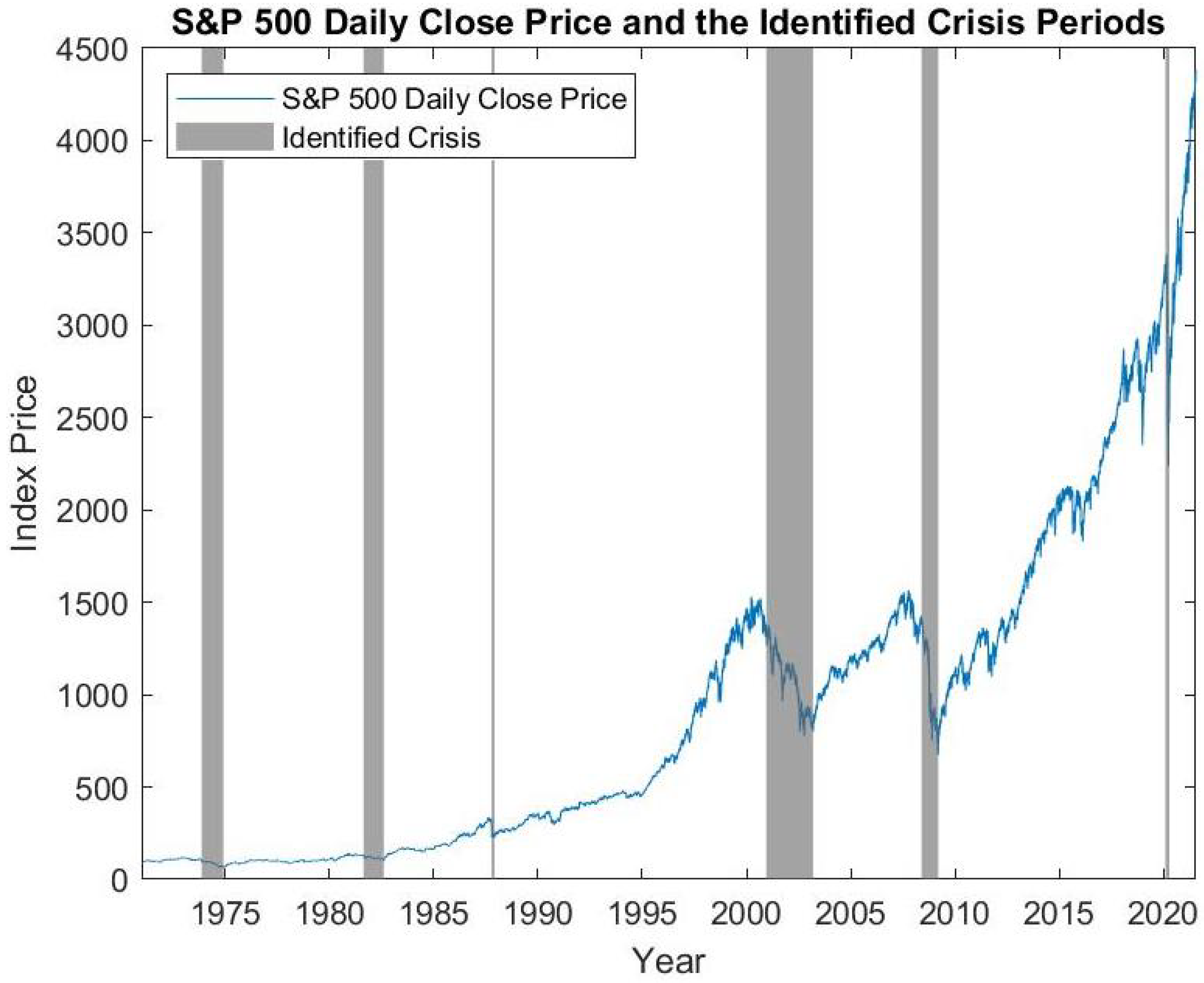
In our application, the examined index time series consists of the daily closing prices of the S&P 500 index from 1 January 1971 to 31 May 2021. The S&P 500 index and the determined crisis periods based on the described method are shown in Figure 1. Specifically, six crisis periods are identified: 20 November 1973 to 6 December 1974 (1973 oil crisis), 24 August 1981 to 12 August 1982 (early 1980s recession), 15 October 1987 to 4 December 1987 (Black Monday), 12 December 2000 to 11 March 2003 (burst of the dot-com bubble), 21 May 2008 to9 March 2009 (global financial crisis) and 5 March 2020 to 23 March 2020 (COVID-19 crisis). The identified crisis periods match the crises recognized universally by economists and the public and are considered a reasonable representation of the true crisis periods.
We further transform the crisis days into a parameter for the determination of the crisis months, as many of the input factors we use to train our neural networks are published monthly. We define a month to be in crisis if at least half of the business days in this month are identified as crisis dates.
In the end, out of the 605 observed months, we identify 62 crisis months, which are: December 1973 to November 1974 (12 months), September 1981 to July 1982 (11 months), October 1987 to November 1987 (2 months), December 2000 to February 2003 (27 months), and June 2008 to February 2009 (9 months) and March 2020 (1 month). They represent 10.25% of the total observed months. Together with the remaining 543 non-crisis months, they constitute our targeted time series for the forecast.
3. The Economic and Financial Input Factors
Our aim is to build neural networks that use a set of input factors from different economic and financial categories to make one-month-ahead forecasts for the economic states. We achieve this by mapping the monthly data of the input factors to the economic states in the next month. Ideally, we obtain neural networks that can identify the hidden structure of the data as well as the underlying relationship between the factors and the economic states, which then provide reliable one-month-ahead forecasts when we include new data in the future.
Our original list, which contains 25 micro- and macroeconomic and financial factors, is an adapted version of the one used in [15] covering the period from December 1970 to April 2021. Based on standard stationarity and correlation checks, we make a few adjustments to the data, e.g., using the relative change of a factor or differences between two factors instead of the original values. In the end, we develop the list comprised of 25 input factors shown in Table 1. Last, but not least, to ensure efficient training, we take the min-max standardized values of these series, which are scaled into the range between 0 and 1 (see [23]).
4. Model Building with Neural Networks
With the time series of the economic and financial factors, as well as the determined crisis months in hand, we build our forecast models comprised of multiple applications of neural networks. These models use the monthly economic and financial factors as input and the one-month-ahead economic states as output. Where monthly data is not available, or there is a time lag in publication, we consider this by only using data which was already available at the beginning of the corresponding forecasting period. This means we only use data which was already available at the beginning of the period for each forecast. On the one hand, it is our aim to select a model which captures the most important economic aspects. On the other hand, we want to reduce the total number of input factors from the data set to avoid overfitting. With 24 variables under consideration, there are, for example, more than 1.9 million model combinations with 10 selected input factors. In addition, one needs to determine an appropriate number of variables to be selected. Hence, it is not practicable to check all possible combinations. To overcome this problem, we suggest a successive input factor selection approach. In the following section, we introduce the structure and the training process of the neural networks which we use. In Section 4.2, we describe the input factor selection procedure.
4.1. Structure of the Neural Networks
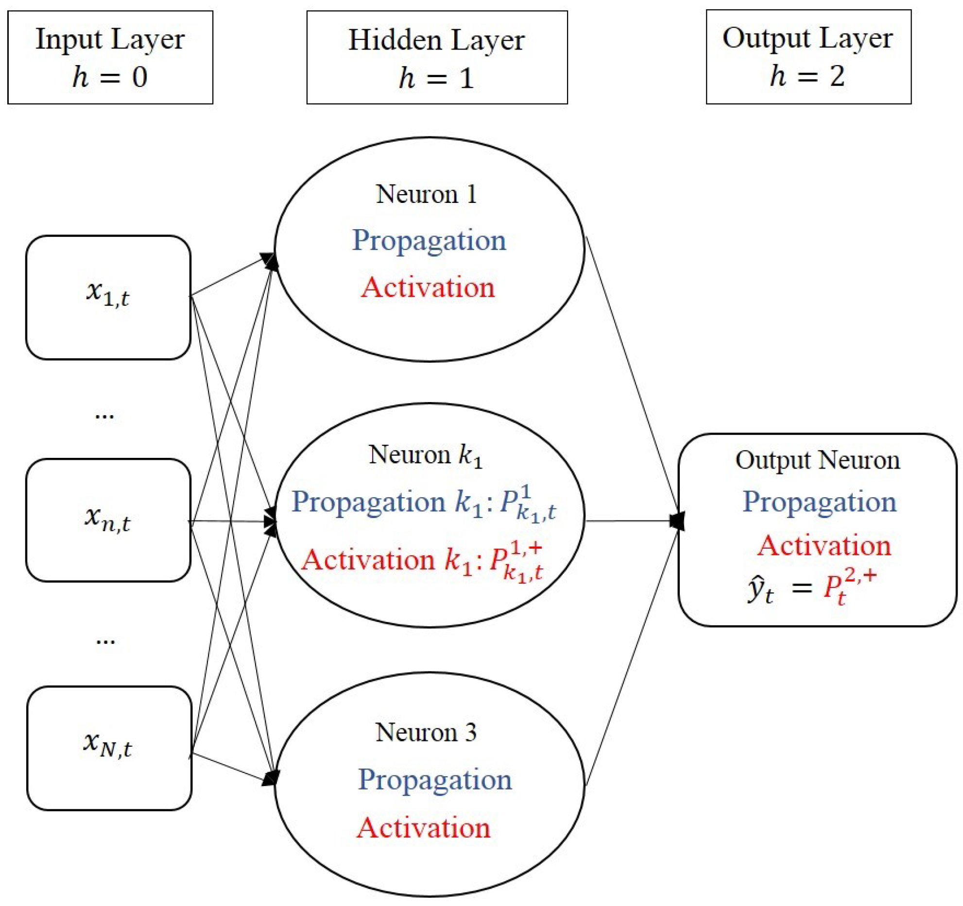
Throughout the model-building process, we use feed-forward neural networks with one input layer, one hidden layer with three neurons, and one output layer. Our neural networks are built from a data set with the following specifications:
- The monthly economic states, as defined and determined in Section 2, are our targeted output variable . The realizations of form a vector . We conduct a binary classification, so Y only takes the values 0 and 1. Furthermore, we have months for the total data set. For the walk-forward forecasting and testing, we train neural networks for different values of T, i.e., also for shorter periods.
- The monthly transformed values of the input factors, as listed in Table 1, are our input variables . The realizations of form a matrix , where , are the input factors given to the neural network to train. Within our model-building approach, we train neural networks with various values for N, i.e., for different subsets of our total set of input factors.
Figure 2 visualizes our neural networks at a time .
The training of a feed-forward supervised neural network starts with forward-feeding. Forward-feeding works in the direction input layer - hidden layer - output layer on the training dataset (see, e.g., [23]). In this step, at each neuron of the hidden layer and the output layer, propagation functions and activation functions are applied as follows:
- At the hidden layer ():
- (a)
- At neuron , we obtain a representation of the input values via the propagation function for each :where is the weight between the n-th input variable and the -th neuron of the hidden layer.
- (b)
- Then, the activation function at this layer, for which we take the rectified linear unit function (ReLU), processes and returns the output of the neuron :where denotes the bias at the neuron .
- At the output layer (), the outputs from the neurons of the previous hidden layer are treated as the inputs for the respective propagation functions. Therefore:
- (a)
- At the output neuron, the propagation function has the form:where is the weight for the -th neuron of the hidden layer.
- (b)
- Then, the sigmoid activation function at this neuron processes and returns the final output of this neuron:
After obtaining the final output at a time , we use a binary cross-entropy loss function to measure the losses between the outputs from the neural network, , and the real observation of the state-identifier, . Since there are far more non-crisis dates than crisis dates, our classification problem is not well-balanced and there is the risk that the crisis dates are not sufficiently taken into account during the fitting process. This is crucial as a crisis forecasting system should work in a reliable way, in particular in times of crises. To overcome this problem, we use a weighted binary cross-entropy loss function (see, e.g., [24]), defined as:
where is either 0 or 1, indicating which state the real observation is in, and the output from the neural network can be interpreted as the probability that this instance is predicted to be in state 1. and are the weights. Setting a higher value for the weight of the class to which less data points belong punishes missed classifications in this class. In our case, we have less crisis dates (class 1) than non-crisis dates (class 0). In order to prevent the non-crisis dates dominating the training, we set a higher weight for than for . We choose these weights to be inversely proportional to the number of data points of the corresponding class in the data set (see, e.g., [25]).
We utilize the commonly used back-propagation to minimize the losses from the weighted binary cross-entropy loss function. Back-propagation computes the gradient of the loss function at each neuron with respect to its weights and biases, and then updates its weights and biases by subtracting the product of the gradient and the learning rate from them (see, e.g., [23]).
4.2. Input Factor Selection Process
Due to the huge number of ways to choose many input factors appropriately from the whole set, we design the selection process in the following way:
- Ranking of the input factors in a successive procedure.
- Selecting the number of input factors in the final model.
4.2.1. Ranking of the Input Factors
There are two possible ways to design such a ranking procedure: either by starting with a model which includes all input factors and by successively pruning variables which contribute the least to the predictive power, or by starting with an empty model and adding the most promising input factors successively. The method of reducing the model with all input factors requires us to fit a very large model to start with. Given the limited horizon of the time series, such a model might suffer from overfitting. Therefore, we proceed by successively adding variables to a model, which is empty in the beginning. In addition, this approach provides the possibility of starting with a set of predetermined input factors, which is then extended. We use this property for an additional model build-up, in which we start with the set of input factors from [15] and extend this set further. To create the ranking of the input factors, we proceed in the following way: The set of the time series of the input factors is given by . For simplicity, we identify the N input factors with the set of their indices and denote the set of input factors which is already chosen for the model by . In the beginning, we set for the approach which starts with an empty model. If we have predefined input factors, which shall definitely be part of the final model, we set S to be the corresponding subset of . The ranking is then done in the following way:
- For each , we fit a neural network with input factors .
- The input factor which leads to the model with the lowest value of the loss function in the previous step is added to S.
These steps are repeated until , i.e., until all input factors are added to the model. The ranking of the input factors is then determined as the order in which the factors were added.
While our approach avoids over-fitting due to too many input factors, it does not completely solve the problem of running into local minima when training the neural networks. Therefore, we propose to improve the credibility and stability of the model by combining it with an ensemble method. This aggregation method often delivers improved accuracy over an individual model and provides better insight into the dataset and the problem (see, e.g., [26,27,28]). While ensemble methods were originally designed to aggregate the output of separately trained models to form one unified prediction (see, e.g., [29]), we adapt the concept to the task of variable selection. We include this idea by conducting the selection process for several random seeds. The total ranking of an input factor is then the average of its rankings across all seeds. We denote the total ranking of input factor by . Then, we sort and re-index the input factors in ascending order, such that:
Using this process, we have determined an order in which the input factors should be added to the model, where the input factor with the lowest total ranking number is the one to be added first. However, in the end, we want to obtain a model which does not include all input factors. We deal with this aspect in the following section.
4.2.2. Selecting the Number of Input Factors in the Final Model
With the total ranking given, we need to determine a point in the ranking from which we do not include the input factors with a worse ranking anymore.
We adapt the largest gap method for determining which input variables can be pruned from the list. This method, suggested by [17], can prune a list of variables instead of a single variable at a time. In [17], the authors first design several measures of sensitivity. Afterwards, they propose the largest gap method based on the measures of sensitivity, which paves the way for efficient variable-pruning in a large batch instead of an one-by-one exclusion. We apply the method to our total rankings instead of sensitivities as in [17].
We define the measure of gap as:
and find the largest gap:
as well as the input factor that presents the largest gap by:
If the outputs for the several seeds at the beginning of the list are very similar (which is a desired outcome), it could happen that the largest gap comes forth already in the first factors on the sorted list (Equation (12)). As a result, we suggest that we take the input factor which presents the largest gap, , upon fulfillment of the criterion that . Alternatively, we would check the second largest gap, third largest gap etc. We define the associated cut factor as . We choose the minimum number of factors to be at least six as [15] have identified six factors in their model.
5. Application of the Model Selection Procedure
We implement the described model selection process in this section and we test the results in Section 6. A common split of the data set into a training, validation and test data set would not suit the nature of time series forecasting, for which one would naturally use all information available from the past to forecast one future period (see, e.g., [30]). As it is our aim to present the best model with respect to all information available, rather than an outdated model, we train the models based on the whole data set (January 1971 until May 2021) for the input factor selection. Note that, with the limited number of data points (only 62 crisis months), a typical training/validation split would not be feasible. With the finally chosen model, we perform out-of-sample forecasts on a rolling basis in Section 6. Using these forecasts, we ensure that the presented model provides good results out-of-sample. Therefore, this procedure is able to fulfill the purpose of the validation and testing. Each of the neural networks is trained for 500 epochs, where we use batch sizes of 32 samples. This means that we only take 32 randomly chosen time points into consideration at once when calculating the gradient of the loss function and subsequently the updates of the weights and biases. Repeating this procedure, while excluding the time points which were already used, one epoch is over when every time point has been considered. In the next epoch, we start the same process as before, beginning again with 32 random samples from the whole time series.
We apply the whole model selection and testing approach to two examples. In the first example, we start with an empty model, so we have initially. We denote this model as Model 1. In this example, we use the variable list from Table 1 except for the term spread of the 5-year government bonds versus the federal funds rate, as this factor is highly correlated with the term spread of the 10-year government bonds versus the federal funds rate. Including highly correlated input variable in the process creates the risk that one of the factors gets a very good ranking and one of the factors gets a very bad ranking. If this happens for some seeds, but for other seeds in reverse order, there is the possibility that none of the factors is chosen as a final input factor though both factors individually would be very good. For completeness, we mention that this is not a problem in our case. As we see later, the term spread of the 10-year government bonds versus the federal funds rate is not represented in the final model. In the second example, we use the input factors determined by [15] as a starting set S. In this example, denoted as Model 2, we do not exclude the term spread of the 5-year government bonds versus the federal funds rate as both term spreads are among the factors proposed by [15]. The authors of [15] argue that including both factors captures the concavity of the term structure rather than the steepness. However, adding the numerically calculated convexity of the term structure as an input factor could not improve the model in our case.
The order of the input factors with respect to their total rankings is determined based on model build-ups with 10 seeds in each of the two models. This can be seen in Table 2 for Model 1 and in Table 3 for Model 2. The associated gaps are also listed in the corresponding tables. As expected, the largest gaps appear at the top of the tables. This means that the corresponding factors are consistently on top of the list across the several seeds. In Table 2, we can observe that the volatility is chosen as the most important factor by the models from almost all seeds with an average rank of 1.1. However, the high numbers above 20 for the last input factors show that these input factors were consistently regarded as less important. In total, the large variety of the total rankings shows that the random variable selection process exhibits good stability. Based on our criterion to choose the largest gap provided that at least six factors are included in the model, we choose , i.e., the last variable which is included in the final model is the change in the federal government debt (GFDEBTN Change). Thus, our final model consists of nine input factors. Performing a principal component analysis, we discover that the first nine principal components explain 89.7% of the total variance in the data set. This gives us an indication that choosing nine variables enables us to capture the main characteristics of the data set well. The chosen input factors reflect various aspects of the financial market and the economy. The volatility (Volatility), the exchange rate (EURODOLLAR) and the federal funds rate (FEDFUNDS) capture different areas of the financial market, namely the stock market, international influences and the central bank policy. The product manufacturing index (PMI) reflects the current situation of companies, while the consumer sentiment index (UMSCENT), the personal savings rate (PSAVERT) and the housing starts (HOUST) incorporate the situation of the households. The unemployment rate (UNRATE) can be interpreted as a factor, in which information on consumers and companies is included. Finally, the change in the government debt (GFDEBTN Change) reflects governmental action. For Model 2, we observe that the first two gaps are given by 2.12 and 1.28 (see Table 3). While the largest gap occurs after the first variable, we decide to cut the factors in this model after the second variable which is added (UMSCENT) for two reasons: first, such a large gap does not occur later anymore, second, the model has eight input factors in total, which makes it comparable to the model selected from Table 2, which has nine input factors. Later, we use Model 2 primarily as a benchmark for Model 1. This means, we add two input factors in Model 2—the unemployment rate (UNRATE) and the consumer sentiment index (UMSCENT). While the model from [15] consists largely of financial market indicators, these two additional factors add information on consumer sentiment (UMSCENT) and the unemployment rate which includes information on consumers and companies. In the following, we assess the quality of the out-of-sample predictions for these models. Model 1 represents our suggested input factor selection process. Model 2 serves as a benchmark as it represents a model which is largely chosen by another input factor selection process and is only extended by our approach.
6. Walk-Forward Forecasting and Testing
Walk-forward forecasting and testing examines the model on a rolling-forward basis (see, e.g., [30]). This method utilizes the historical data up to the observed time point to fit the neural network at this time and tests the network’s forecasting performance (classification accuracy) comparing the forecasting result for the next time point with the corresponding crisis classification as determined in Section 2. When the observation of the next time point becomes available, the same process is repeated with the same set of input factors and a data set containing one extra observation. As our point of observation moves forward in time, we continue to acquire more and more historical data to fit our most up-to-date neural networks, as well as more testing results from the new single tests. In the end, we investigate the testing results over time to analyze the performance of a series of neural networks, which reinforces the check on the suitability and effectiveness of the neural network series’ prescribed architecture and specifications.
Compared to fixed training/test splits, walk-forward testing suits the nature of a time series prediction better, but it requires us to train the neural network at each time point. Of course, the period for the walk-forward forecasting and testing should be set long enough to cover different market situations, such as calm periods and crises. We choose January 2000 as our starting point for the walk-forward forecasting and testing, meaning that the first model is trained with the data up to December 1999 (denoted by ) and with the data available at the end of December; the first forecast which we create is the one for January 2000. This division ensures that we have enough representations of both classes for training and for testing the predictions, as it grants 25 crisis months for the first model estimation and allows, in total, 37 crisis months for the subsequent testing up to the end of the final tests. Then, we obtain 257 successively estimated neural networks, each trained at time , and tested with the next available data at time , respectively. This means that each forecast is an out-of-sample prediction.
It is the core principle of walk-forward testing that, after each month, the model is adjusted to incorporate the newest information. On the other hand, the new information from adding only one month is very little compared to the rest of the information, as the older time points stay the same. Therefore, we should expect only a small change in the model from one month to another, while the change over a longer period can be substantial. To incorporate the characteristics of this data structure, we propose a modified walk-forward testing method that incorporates multiple global estimations as well as sequential estimations. We conduct global estimations once every 48 months and sequential estimations monthly between the global estimations. At each global estimation, we train the model for 750 epochs, where we use a batch size of 32 time points. At each sequential estimation, we train the model for 500 epochs. During the global estimations, the neural network is trained with neutral starting values for the parameters. Then, for the sequential estimations, we take the parameters of the previous model as starting values and we train the neural network based on the new input data set with the newest month added. After each globally-estimated neural network is rebuilt and retrained, sequential estimations follow until the next global estimation. The sequential estimations take advantage of the previous results and the fact that the input data set does not change much each month, whereas the global estimations prevent the model from being stuck in a local minimum, which might become more unfavorable as the data set grows.
Again, we use an ensembling method: all trainings and predictions are performed for 10 different seeds. As an output, we receive, for each neural network, numbers between 0 and 1, which can be interpreted as probabilities for a crisis. We define that an ensemble predicts a crisis if the average probability to be in the crisis state across all seeds is at least 50%. The results of the predictions are listed in Table 4. We observe that Model 1 outperforms Model 2 with respect to all aspects. In particular, we see that Model 1 is good at predicting crisis states accurately, as only 3 of the 37 crisis months are missed. For an early warning system, the ability to predict times of crises is crucial. This is an aspect in which Model 1 very significantly outperforms Model 2, which detects only 56.8% of the crisis months. Model 1 succeeds here by recognizing 91.9% of the crisis months. On the other hand, the classification of non-crisis states, for which our model succeeds in 90.5% of the cases, does not suffer from its good crisis prediction properties. The strength of our model selection approach becomes even clearer when we compare the results to a walk-forward forecasting and testing approach for a model which uses the nine factors with the worst ranking from Table 2. Such a model only predicts 19 of the 37 crisis months correctly (51.4%) and achieves a total accuracy of 72.8%.
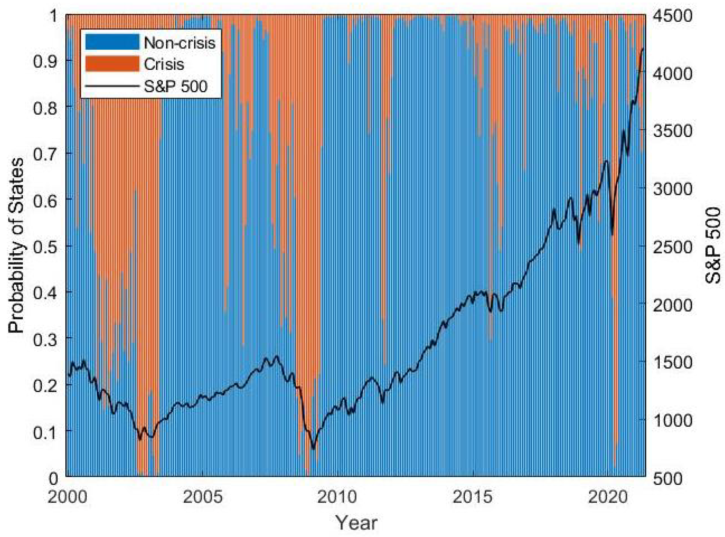
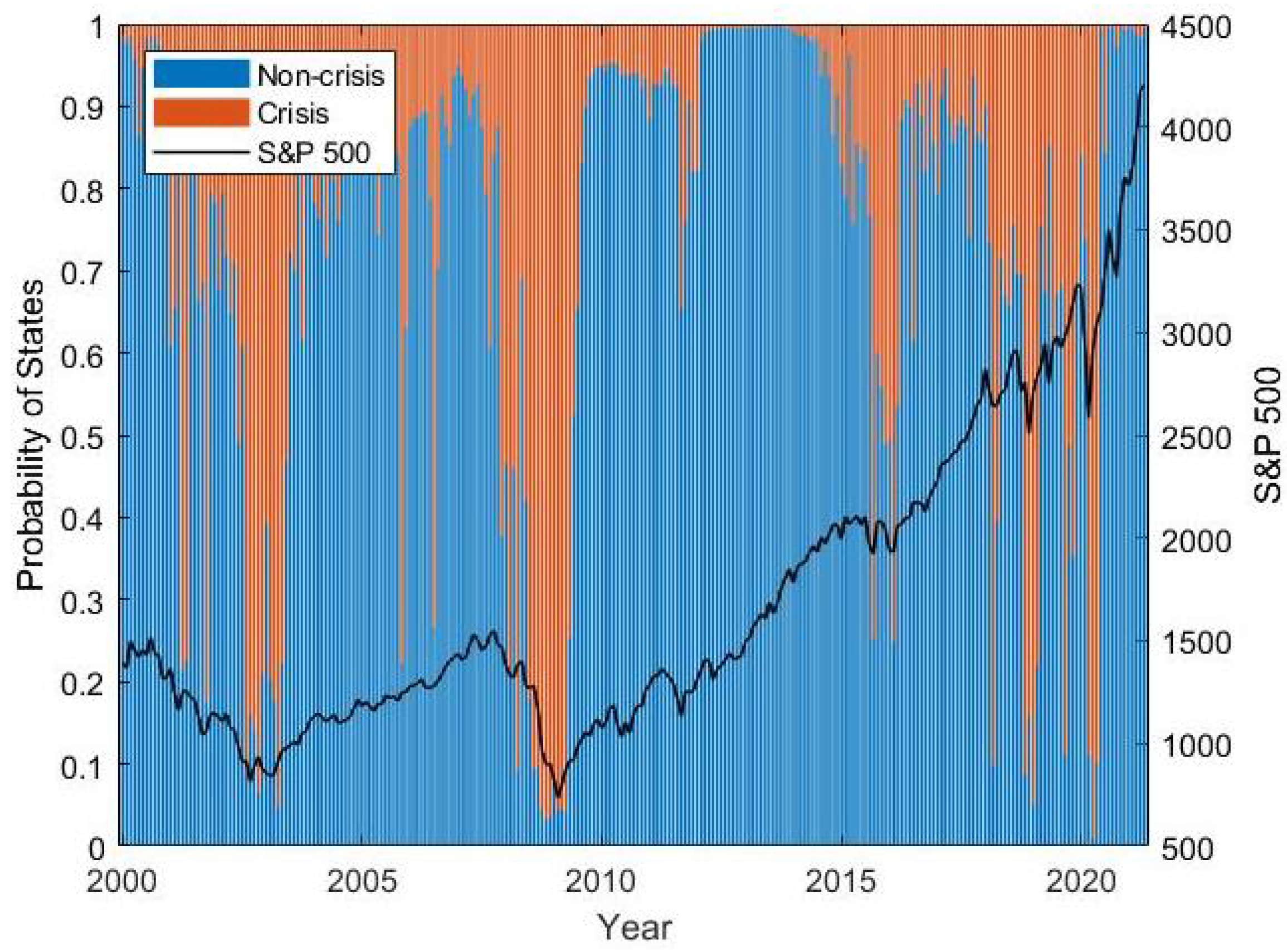
Figure 3 and Figure 4 show the average predicted probability over all seeds for each point in time. With the method from Section 2, three crises have been identified after year 2000, which took place from December 2000 to February 2003, from June 2008 to February 2009 and in March 2020. We see that both models capture all of these crises. Moreover, we see that the models also detect the end of the crises in a timely manner. In addition, we can observe that both models also recognize smaller stock market setbacks which are not part of these crisis periods and that, during these setbacks, the probability for a crisis is not as high as during a major crisis. This is a remarkable feature as the models were neither directly selected nor directly trained with respect to setbacks outside major crisis periods. A possible reason for this behavior might be that patterns in financial markets are similar in times of setbacks and in crisis periods, but they are observed to a smaller extent in smaller setbacks. Comparing Figure 3 and Figure 4, we see that both models exhibit similar behavior, but Model 1 separates crisis times and non-crisis times in a more distinctive way.
In total, the walk-forward testing shows that our model-building process has successfully built neural networks that continuously make reliable out-of-sample forecasts of financial crises. It also demonstrates an improvement of performance compared to a traditional model selection method, represented by Model 2 in our example.
7. Conclusions
In this article, we explore the potential of neural networks for forecasting financial crises with micro-, macroeconomic and financial factors. In order to minimize the input dimension, we develop an input variable reduction method based on a successive selection procedure combined with a largest gap analysis.
We demonstrate the model-building process with the forecast of crises determined from the S&P 500 index. The walk-forward testing shows that our approach is able to create models which make reliable out-of-sample, one-month-ahead forecasts. We also observe that our model outperforms a model which consists largely of input factors taken from [15]. Our procedure overcomes different shortcomings which are typically attributed to stock market early warning systems based on neural networks. Among these are the problems of over-fitting and unstable models, as described in [2,3]. Although, we do not need to select input factors based on expert knowledge, such as in [16], their model and ours have in common that various segments of the financial markets are considered as an input to forecast a crisis. Furthermore, we present an alternative to a selection based on sensitivities (see [17,18]). Our approach suits financial input data sets that include variables with only minor changes from one period to another. but with larger effects over an economic cycle. The common strength of the input sensitivity approach and our approach, however, is that both procedures utilize a gap method to prune a whole set of variables at once.
With the research area on the applications of neural networks being so dynamic, several questions for further research emerge. Possible extensions of our input factor reduction approach to comprise more involved structures, such as recurrent neural networks, might be interesting. Furthermore, while we focus on forecasting financial crises, the question arises how our model can be used for specific tasks, such as risk and portfolio management and the construction of quantitative investment strategies.
Author Contributions
Conceptualization, M.W. and R.Z.; methodology, F.F., M.W., R.Z. and X.Z.; software, F.F. and X.Z.; writing—original draft preparation, M.W. and X.Z.; writing—review and editing, F.F., M.W., R.Z. and X.Z., supervision, M.W. and R.Z. All authors have read and agreed to the published version of the manuscript.
Funding
This research received no external funding.
Institutional Review Board Statement
Not applicable.
Informed Consent Statement
Not applicable.
Conflicts of Interest
The authors declare no conflict of interest.
Appendix A. Sources of the Input Factors

Table A1.
Sources of the Input Factors. Accessed in 20 June 2021.
References
- Gallo, C.; Letizia, C.; Stasio, G. Artificial neural networks in financial modelling. In Proceedings of the XXXVI EWGFM International Meeting “European Working Group on Financial Mathematics”, Brescia, Italy, 5–7 May 2005; pp. 5–7. [Google Scholar]
- Feng, G.; He, J.; Polson, N.G. Deep learning for predicting asset returns. arXiv 2018, arXiv:1804.09314. [Google Scholar]
- Heaton, J.B.; Polson, N.G.; Witte, J.H. Deep learning for finance: Deep portfolios. Appl. Stoch. Model. Bus. Ind. 2017, 33, 3–12. [Google Scholar] [CrossRef]
- Obthong, M.; Tantisantiwong, N.; Jeamwatthanachai, W.; Wills, G. A Survey on Machine Learning for Stock Price Prediction: Algorithms and Techniques. In Proceedings of the 2nd International Conference on Finance, Economics, Management and IT Business, Online, 5–6 May 2020; pp. 63–71. [Google Scholar] [CrossRef]
- Wang, P.; Zong, L. Are Crises Predictable? A Review of the Early Warning Systems in Currency and Stock Markets. arXiv 2020, arXiv:2010.10132. [Google Scholar]
- Atsalakis, G.S.; Valavanis, K.P. Surveying stock market forecasting techniques—Part II: Soft computing methods. Expert Syst. Appl. 2009, 36, 5932–5941. [Google Scholar] [CrossRef]
- Dixon, M.; Klabjan, D.; Bang, J.H. Implementing deep neural networks for financial market prediction on the Intel Xeon Phi. In Proceedings of the 8th Workshop on High Performance Computational Finance, Austin, TX, USA, 15 November 2015; pp. 1–6. [Google Scholar]
- Lee, S.I.; Yoo, S.J. A deep efficient frontier method for optimal investments. arXiv 2017, arXiv:1709.09822. [Google Scholar]
- Jiang, Z.; Xu, D.; Liang, J. A deep reinforcement learning framework for the financial portfolio management problem. arXiv 2017, arXiv:1706.10059. [Google Scholar]
- Pacelli, V.; Bevilacqua, V.; Azzollini, M. An Artificial Neural Network Model to Forecast Exchange Rates. J. Intell. Learn. Syst. Appl. 2011, 3, 57–69. [Google Scholar] [CrossRef] [Green Version]
- Escudero, P.; Alcocer, W.; Paredes, J. Recurrent Neural Networks and ARIMA Models for Euro/Dollar Exchange Rate Forecasting. Appl. Sci. 2021, 11, 5658. [Google Scholar] [CrossRef]
- Pukała, R. Use of Neural Networks in Risk Assessment and Optimization of Insurance Cover in Innovative Enterprises. Ekonomia i Zarzadzanie 2016, 8, 43–56. [Google Scholar] [CrossRef] [Green Version]
- Sarcià, S.A.; Cantone, G.; Basili, V.R. A statistical neural network framework for risk management process. In Proceedings of the ICSOFT, Barcelona, Spain, 22–25 July 2007. [Google Scholar]
- Hamilton, J.D. A New Approach to the Economic Analysis of Nonstationary Time Series and the Business Cycle. Econometrica 1989, 57, 357–384. [Google Scholar] [CrossRef]
- Hauptmann, J.; Hoppenkamps, A.; Min, A.; Ramsauer, F.; Zagst, R. Forecasting market turbulence using regime-switching models. Financ. Mark. Portf. Manag. 2014, 28, 139–164. [Google Scholar] [CrossRef]
- Oh, K.; Kim, T.; Kim, C. An early warning system for detection of financial crisis using financial market volatility. Expert Syst. 2006, 23, 83–98. [Google Scholar] [CrossRef]
- Zurada, J.M.; Malinowski, A.; Cloete, I. Sensitivity analysis for minimization of input data dimension for feedforward neural network. In Proceedings of the IEEE International Symposium on Circuits and Systems, London, UK, 30 May–2 June 1994; pp. 447–450. [Google Scholar] [CrossRef]
- Engelbrecht, A.P. A new pruning heuristic based on variance analysis of sensitivity information. IEEE Trans. Neural Netw. 2001, 12, 1386–1399. [Google Scholar] [CrossRef] [PubMed]
- Zeng, X.; Yeung, D.S. Sensitivity analysis of multilayer perceptron to input and weight perturbations. IEEE Trans. Neural Netw. 2001, 12, 1358–1366. [Google Scholar] [CrossRef] [PubMed]
- Ernst, C.; Grossmann, M.; Hocht, S.; Minden, S.; Scherer, M.; Zagst, R. Portfolio selection under changing market conditions. Int. J. Financ. Serv. Manag. 2009, 4, 48–63. [Google Scholar] [CrossRef]
- Min, A.; Scherer, M.; Schischke, A.; Zagst, R. Modeling Recovery Rates of Small- and Medium-Sized Entities in the US. Mathematics 2020, 8, 1856. [Google Scholar] [CrossRef]
- Bernhart, G.; Höcht, S.; Neugebauer, M.; Neumann, M.; Zagst, R. Asset correlations in turbulent markets and the impact of different regimes on asset management. Asia-Pac. J. Oper. Res. 2011, 28, 1–23. [Google Scholar] [CrossRef]
- Beysolow, T., II. Introduction to Deep Learning Using R; Apress: Berkeley, CA, USA, 2017. [Google Scholar] [CrossRef]
- Ho, Y.; Wookey, S. The Real-World-Weight Cross-Entropy Loss Function: Modeling the Costs of Mislabeling. IEEE Access 2020, 8, 4806–4813. [Google Scholar] [CrossRef]
- Cui, Y.; Jia, M.; Lin, T.Y.; Song, Y.; Belongie, S. Class-balanced loss based on effective number of samples. In Proceedings of the IEEE/CVF Conference on Computer Vision and Pattern Recognition, Long Beach, CA, USA, 15–20 June 2019; pp. 9268–9277. [Google Scholar]
- Qiu, X.; Zhang, L.; Ren, Y.; Suganthan, P.; Amaratunga, G. Ensemble deep learning for regression and time series forecasting. In Proceedings of the 2014 IEEE Symposium on Computational Intelligence in Ensemble Learning (CIEL), Orlando, FL, USA, 9–12 December 2014; pp. 1–6. [Google Scholar] [CrossRef]
- Jimenez, D. Dynamically weighted ensemble neural networks for classification. In Proceedings of the 1998 IEEE International Joint Conference on Neural Networks Proceedings, Anchorage, AK, USA, 4–9 May 1998; pp. 753–756. [Google Scholar] [CrossRef]
- Krogh, A.; Vedelsby, J. Neural network ensembles, cross validation and active learning. In Proceedings of the Advances in Neural Information Processing Systems, Denver, CO, USA, 28 November–1 December 1994. [Google Scholar]
- Dietterich, T.G. Ensemble Methods in Machine Learning. In Multiple Classifier Systems; Springer: Berlin/Heidelberg, Germnay, 2000; pp. 1–15. [Google Scholar]
- Kaastra, I.; Boyd, M. Designing a neural network for forecasting financial and economic time series. Neurocomputing 1996, 10, 215–236. [Google Scholar] [CrossRef]
Figure 1.
S & P 500 Daily Closing Price and Identified Crisis Periods.

Figure 2.
Feed-forward neural network with one hidden layer.

Figure 3.
One-month-ahead predictions for Model 1.

Figure 4.
One-month-ahead predictions for Model 2.

Table 1.
Complete Variable List Before Input Factor Reduction (see Appendix A, Table A1 for the data sources).
Table 1.
Complete Variable List Before Input Factor Reduction (see Appendix A, Table A1 for the data sources).
| Abbreviation | Variable Description |
|---|---|
| BAA-AAA | Difference: Moody’s Seasoned Baa vs. AAA Corporate Bond Yield |
| CPIAUCSL Change | Relative change of the Consumer Price Index for All Urban Consumers: All Items |
| FEDFUNDS | Effective Federal Funds Rate |
| GS5-FEDFUNDS | Difference: 5-Year Treasury Constant Maturity Rate vs. Effective Federal Funds Rate |
| GS10-FEDFUNDS | Difference: 10-Year Treasury Constant Maturity Rate vs. Effective Federal Funds Rate |
| HOUST | Housing Starts: Total: New Privately Owned Housing Units Started |
| INDPRO Change | Relative change of the Industrial Production Index |
| M1NS Change | Relative change of the M1 Money Stock |
| M2NS Change | Relative change of the M2 Money Stock |
| OECD CLI | Composite leading indicator for OECD + 6 major non-member economies |
| PAYEMS Change | Relative change of the All Employees: Total Nonfarm Payrolls |
| PMI | ISM Manufacturing: PMI Composite Index |
| PPIACO Change | Relative change of the Producer Price Index for All Commodities |
| PSAVERT | Personal Saving Rate |
| TCU | Capacity Utilization: Total Industry |
| TOTALSL Change | Relative change of the Total Consumer Credit Owned and Securitized, Outstanding |
| TRESEGUSM052N Change | Relative change of the Total Reserves excluding Gold for United States |
| UMCSENT | University of Michigan: Consumer Sentiment |
| UNRATE | Civilian Unemployment Rate |
| VOLATILITY | Historical 20-day volatility of the S&P 500 |
| W823RC1 Change | Relative change of government social benefits to persons |
| WTISPLC Change | Relative change of the Spot Crude Oil Price: West Texas Intermediate (WTI) |
| GDP Quarterly Change | Relative quarterly change of the Gross Domestic Product |
| GFDEBTN Change | Relative change of the Federal Debt: Total Public Debt |
| EURO-DOLLAR | Euro to US Dollar exchange rate |
Table 2.
Selection with initial (Model 1).
| Variable | Average Ranking | Gap to Next Factor |
|---|---|---|
| Volatility | 1.1 | 4 |
| PMI | 4.4 | 1.05 |
| EURODOLLAR | 4.6 | 1 |
| UMCSENT | 4.6 | 1.3 |
| UNRATE | 5.8 | 1.31 |
| FEDFUNDS | 7.6 | 1.07 |
| PSAVERT | 8.1 | 1.05 |
| HOUST | 8.5 | 1.01 |
| GFDEBTN Change | 8.6 | 1.3 |
| BAAMinusAAA | 11.0 | 1.08 |
| M3 Change | 11.9 | 1.06 |
| GS10MinusFEDFUNDS | 12.6 | 1.09 |
| TCU | 13.7 | 1.03 |
| PPIACO Change | 14.1 | 1.04 |
| TOTALSL Change | 14.7 | 1.05 |
| WTISPLC Change | 15.5 | 1.02 |
| PAYEMS Change | 15.8 | 1.13 |
| CPIAUCSL Change | 17.8 | 1 |
| W823RC1 Change | 17.8 | 1.01 |
| GPD Change | 18.0 | 1.08 |
| TRESEGUSM025N Change | 19.4 | 1.04 |
| INDPRO Change | 20.2 | 1 |
| OECD CLI | 20.2 | - |
Table 3.
Input factors from [15] in S initially (Model 2).
Table 3.
Input factors from [15] in S initially (Model 2).
| Variable | Average Ranking | Gap to Next Factor |
|---|---|---|
| BAAMinusAAA | - | - |
| FEDFUNDS | - | - |
| GS5MinusFEDFUNDS | - | - |
| GS10MinusFEDFUNDS | - | - |
| OECD CLI | - | - |
| Volatility | - | - |
| UNRATE | 1.7 | 2.12 |
| UMCSENT | 3.6 | 1.28 |
| EURODOLLAR | 4.6 | 1.04 |
| PSAVERT | 4.8 | 1.15 |
| GFDEBTN Change | 5.5 | 1.16 |
| HOUST | 6.4 | 1.09 |
| TCU | 7.0 | 1.16 |
| PMI | 8.1 | 1.09 |
| M3 Change | 8.8 | 1.16 |
| PPIACO Change | 9.4 | 1.09 |
| WTISPLC Change | 10.2 | 1.18 |
| TOTALSL Change | 12.0 | 1.13 |
| GPD Change | 13.5 | 1.06 |
| CPIAUCSL Change | 14.3 | 1.05 |
| W823RC1 Change | 15.0 | 1.01 |
| PAYEMS Change | 15.1 | 1.02 |
| TRESEGUSM025N Change | 15.4 | 1.01 |
| INDPRO Change | 15.6 | - |
Table 4.
Results of the walk-forward forecasting and testing.
| Model 1 | Model 2 | |
|---|---|---|
| Correct Forecasts | 233/257 | 212/257 |
| Total Test Accuracy | 90.7% | 82.5% |
| True Positive (TP) | 34/37 | 21/37 |
| False Positive (FP) | 21/220 | 29/220 |
| True Negative (TN) | 199/220 | 191/220 |
| False Negative (FN) | 3/37 | 16/37 |
| TP in % | 91.9% | 56.8% |
| TN in % | 90.5% | 86.8% |
Publisher’s Note: MDPI stays neutral with regard to jurisdictional claims in published maps and institutional affiliations. |
© 2022 by the authors. Licensee MDPI, Basel, Switzerland. This article is an open access article distributed under the terms and conditions of the Creative Commons Attribution (CC BY) license (https://creativecommons.org/licenses/by/4.0/).
Share and Cite
MDPI and ACS Style
Fuchs, F.; Wahl, M.; Zagst, R.; Zheng, X. Stock Market Crisis Forecasting Using Neural Networks with Input Factor Selection. Appl. Sci. 2022, 12, 1952. https://0-doi-org.brum.beds.ac.uk/10.3390/app12041952
AMA Style
Fuchs F, Wahl M, Zagst R, Zheng X. Stock Market Crisis Forecasting Using Neural Networks with Input Factor Selection. Applied Sciences. 2022; 12(4):1952. https://0-doi-org.brum.beds.ac.uk/10.3390/app12041952
Chicago/Turabian StyleFuchs, Felix, Markus Wahl, Rudi Zagst, and Xinyi Zheng. 2022. "Stock Market Crisis Forecasting Using Neural Networks with Input Factor Selection" Applied Sciences 12, no. 4: 1952. https://0-doi-org.brum.beds.ac.uk/10.3390/app12041952
Note that from the first issue of 2016, this journal uses article numbers instead of page numbers. See further details here.