
CTIMS: Automated Defect Detection Framework Using Computed Tomography
by
 , , ,
, , ,
Hossam A. Gabbar
1,2,* ,
,
Abderrazak Chahid
1,
Md. Jamiul Alam Khan
2 ,
,
Oluwabukola Grace Adegboro
2 and
Matthew Immanuel Samson
3 1
Faculty of Energy Systems and Nuclear Science, Ontario Tech University (UOIT), Oshawa, ON L1G 0C5, Canada
2
Faculty of Engineering and Applied Science, Ontario Tech University (UOIT), Oshawa, ON L1G 0C5, Canada
3
New Vision Systems Canada Inc. (NVS), Scarborough, ON M1S 3L1, Canada
*
Author to whom correspondence should be addressed.
Appl. Sci. 2022, 12(4), 2175; https://0-doi-org.brum.beds.ac.uk/10.3390/app12042175
Submission received: 16 December 2021
/
Revised: 11 February 2022
/
Accepted: 14 February 2022
/
Published: 19 February 2022
(This article belongs to the Topic Artificial Intelligence in Smart Industrial Diagnostics and Manufacturing)
Abstract
:Non-Destructive Testing (NDT) is one of the inspection techniques used in industrial tool inspection for quality and safety control. It is performed mainly using X-ray Computed Tomography (CT) to scan the internal structure of the tools and detect the potential defects. In this paper, we propose a new toolbox called the CT-Based Integrity Monitoring System (CTIMS-Toolbox) for automated inspection of CT images and volumes. It contains three main modules: first, the database management module, which handles the database and reads/writes queries to retrieve or save the CT data; second, the pre-processing module for registration and background subtraction; third, the defect inspection module to detect all the potential defects (missing parts, damaged screws, etc.) based on a hybrid system composed of computer vision and deep learning techniques. This paper explores the different features of the CTIMS-Toolbox, exposes the performance of its modules, compares its features to some existing CT inspection toolboxes, and provides some examples of the obtained results.
1. Introduction
Electrical energy is one of the major pillars of the global economy. It can be generated using different resources such as fossil fuels (coal, natural gas, and petroleum), nuclear energy, and renewable energy sources. For instance, in Canada, the shares of the different power resources are split as follows: hydro at , nuclear at , coal at , gas/oil/others at , and non-hydro renewables at [1]. As Canada is the world’s second largest producer of uranium [2] and due to the significant share of nuclear power in the national production, more support is focused on the design as next-generation nuclear energy systems improve its efficiency, such as the CANDU reactor [3]. However, nuclear-based energy is costly due to the high operation cost and extended reactor shutdown durations. These outages are usually caused by periodic maintenance, fault conditions, etc. For instance, the nuclear vault has to stay shut down till all entered objects are manually checked and identified as complete. Therefore, it is important to reduce the maintenance-related outage cost (USD 35 per second USD per outage) by accelerating the tools’ inspection. Different Non-Destructive Testing (NDT) methods have been proposed in the literature to perform tool inspection based on different scanning technologies [4,5]: thermography imaging, radiography techniques, ultrasonic probes, etc. Computerized Tomography (CT) imaging is one of the emerging NDT technologies that has been used in different applications: quality control [6,7], quantitative material analysis [8,9], medicine [10,11], and geosciences [12]. One of the main challenges in CT-based inspection is the presence of artifacts and the limited-angle computed tomography, which reduces the CT data quality. Different research works have focused on improving the CT data quality by improving the scanner configuration, such as the newly optimized reconstruction algorithm [13,14,15]. The existing CT-based defect inspection methods can be classified into two main categories: image-processing-based techniques and deep learning methods. The first category uses signal and image processing techniques to extract the defect’s relevant features or pattern. For instance, this kind of defect inspection is performed using near-net-shape production techniques [16] and the kriging model with statistical models to compute the shape deviation errors [17,18]. The second category uses deep computer vision models trained on a labeled dataset, taking advantage of the rapid progress of this field [19,20,21]. For instance, some approaches use local binary patterns [22], Class-balanced Hierarchical Refinement (CHR) [23], Convolutional Neural Networks (CNNs) [24], and spatial attention bilinear CNNs [25]. However, the performance of the proposed deep learning models depends on the quality and size of the training dataset. At the commercialization level, there exists some X-ray CT-based software for quality control in industrial applications using CT technology such as [26,27,28]. In addition, there are some other hardware–software solutions for automated industrial processes, such as the Carl Zeiss AG [29] and VisiConsult X-ray Systems [30].
In this paper, a new CTIMS-Toolbox is proposed for X-ray Computed Tomography (CT) data inspection. It integrates computer vision techniques and state-of-the-art Artificial Intelligence (AI) models for better external/internal tool integrity. In addition, it uses an automation flowchart to perform the auto-inspection using the integrated techniques with less intervention from the user. The proposed hybrid framework focuses mainly on X-ray-based inspection to detect the structural differences between two input X-ray CT volumes or images. The efficiency of the proposed framework is demonstrated using X-ray data of metallic tools used in nuclear power plants. In addition, the proposed CTIMS-Toolbox can be used for any other non-destructive testing or inspection application based on X-ray data. For instance, it can be used for inspection of aircraft engines, gas and oil industry pipelines, cavity detection in dental diagnosis, etc.
This paper is organized as follows. In Section 2, a general overview of the toolbox framework features and flowchart are given. Section 3 presents the data management module and describes how the CT data and inspection results are managed using a SQL database. Section 4 exposes the integrated pre-processing module and presents the integrated background subtraction and registration functions and their performances. Section 5 presents the defect inspection module containing the defect prediction, localization, and characterization. An example of the obtained inspection results is given in this section. Finally, concluding remarks and future works are summarized in Section 6.
2. CTIMS-Toolbox Framework
The proposed toolbox is a CT scan inspection software integrating data management, data pre-processing, and defect inspection modules. This toolbox obtains X-ray CT scans of an object before and after its use in the vault maintenance. Then, it detects the defects and localizes their positions/locations within this object. Figure 1 shows the framework of X-ray based tool inspection.
The proposed Toolbox GUI contains three main modules:
- Data management module: prepares the raw data coming from the scanner in a SQL database;
- Data pre-processing module: pre-processes and prepares the input CT data (2D images/3D volume) for the inspection step. This module applies two main pre-processing functions: background subtraction and registration;
- Defect inspection module: performs an automated defect inspection based on different computer vision and deep-learning-based inspection algorithms: defect classification, defect localization, and defect characterization.
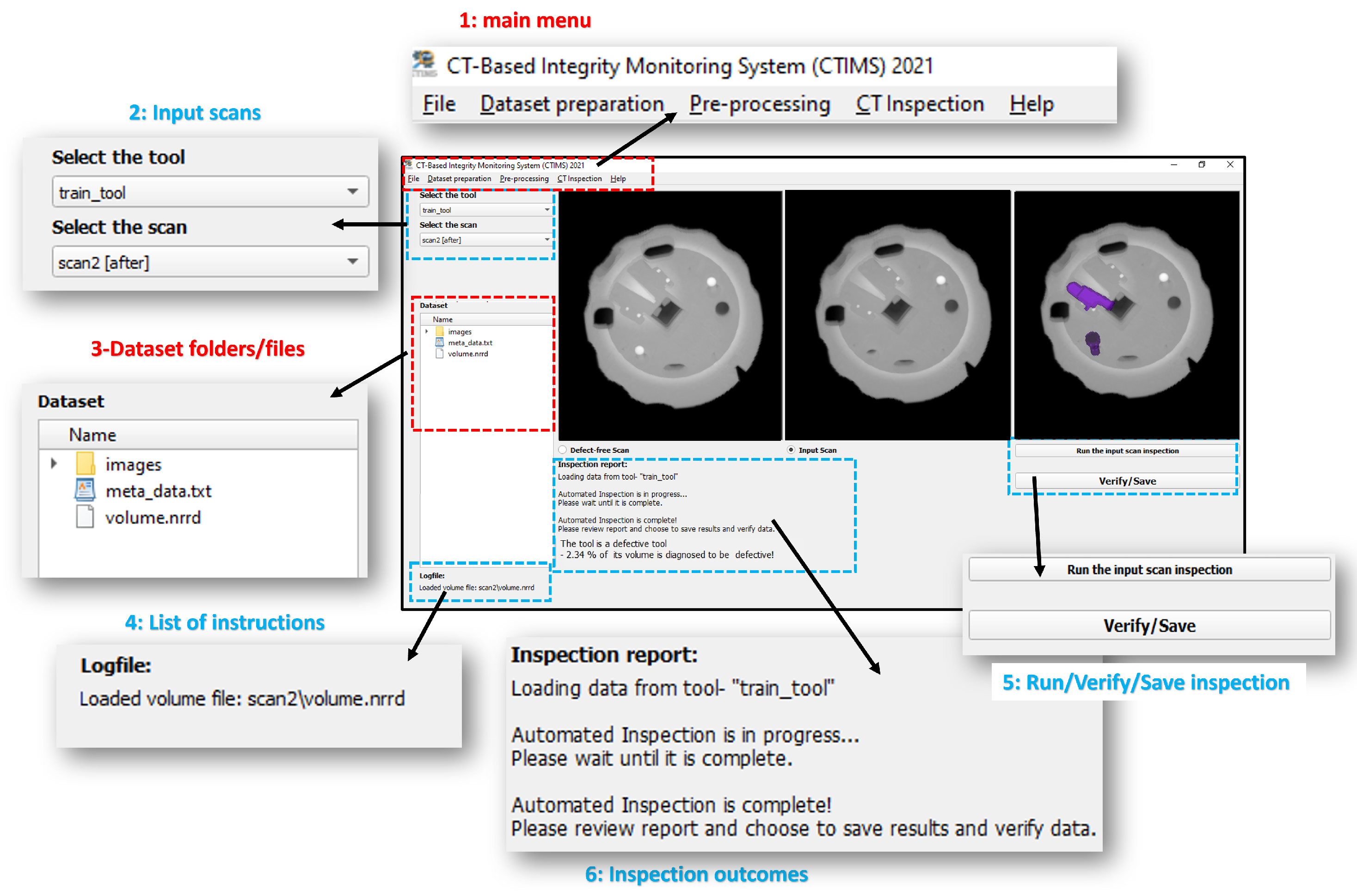
These modules are integrated within the Toolbox user interface using the PyQT Library (see Figure 2).
Thanks to its automated framework, the CTIMS-Toolbox performs the defect inspection with minimal user interactions. This automated framework manages the data exchange between the modules and their interaction with the user, as shown in the following Figure 3.
The different modules of the CTIMS-Toolbox are explained in detail in the following sections.
3. Database Management
The data management module is responsible for handling all required data operations through a custom-built API: data storage and data retrieval. In addition, it manages the needed operations of the different modules of the Toolbox: retrieve customized queries for data pre-processing or data inspection modules, store the pre-processed data, and store the inspection results and the deep learning model. Figure 4 explores the data flow and the user interaction. The deployed database was built using a basic data table structure to store the data vectors: images’ and volumes’ directories, data types, deep learning model configuration parameters, and their respective trained version.
In order to manage the data flow through the different modules of the toolbox, the data management system was implemented in a highly centralized manner to organize and manage data storage and usage. This database structure was implemented using MySQL 8.0 [31]. It is important to note that the MySQL server needs to be installed separately. The created SQL server was configured using the following steps:
- Create a user account using the default username and password;
- Set the server configuration to connect to port 3306 (default port).
The database management systems save the corresponding data in a dedicated folder structure for the tools, scans, and models as follows:
Tool: represents the scanned tool defined by: tool name, CAD files, and metadata describing its properties such as material, volume, etc. In addition, the tool folder contains the scan data as defined in the next element. An example of the tool folder structure is shown in Figure 5a.
Scan: Each scan folder contains the data collected from the X-ray scanner. A scan is defined by: collected projection images, reconstructed volume, and relevant metadata such as image/volume size, scanner configuration, etc.
Inspection object: manages the outputs on the inspection module such as the trained deep learning model version, training configuration parameters, and performance results. An example of the inspection object is shown in Figure 5b.
3.1. SQL Tables’ Structure or Flowchart
The module creates a new database structure considering the core relationship between the tool and its respective connected data (scan). It provides an all-encompassing, flexible, and adaptive knowledge-base that efficiently manages the data queries: load, store, and update. The database is designed based on the following table structure:
- Tool table: describes the tool data, including optional CAD data, stored CAD volume, and object labels;
- Scan table: describes the scan data within a tool and includes all the metadata regarding the particular scan;
- Relate tool scan table: relates the tool with its respective scan data and the locations of the relevant directories;
- Model table: contains all trained models of the deep-learning-based inspection algorithms;
- Relate model version table: stores the trained models and tracks their versions with further training using new data.
The relation between all tables is shown in Figure 6.
3.2. Incremental Model Training
During the deep learning model training phase, the needed data are loaded from the database forming the training set. The training set contains scans selected depending on the model type, the required classes/labels, and the respective tool of interest. Once the training phase is finished, the trained model is saved back to the database with its training parameters and performance results. However, if the trained model did not achieve better/acceptable performance, it will be trained again on a different set of data from the DB if available. This process keeps running till a new, better performance is achieved. The data management module keeps track of all versions of every trained model, including the parameters and performance results. Figure 7 shows the integrated incremental training flowchart.
3.3. Data Management Cycle
The data are usually loaded for visualization and inspection. Then, the outcome/outputs /results of the data usage are always stored back into the database in a closed loop to ensure the traceability of the dataset flow. Figure 8 shows the data flow cycle in the proposed toolbox.
3.4. Limitations
The primary purpose of database management is to control the storage, organization, and loading of the data and algorithms. However, this does not yet address the recent data warehousing and big-data-type structures. Therefore, some limitations encountered are discussed below:
- The automatically generated metadata from the new imported tools or scans are highly dependent on the fact that the user can carefully check the metadata and update this in case of an error.
4. Data Pre-Processing
CT data pre-processing is a critical step in CT inspection as it represents the initial operation to perform on the raw data collected from the CT scanner. This step prepares the 2D or 3D CT data for the next step, such as data storage or CT inspection. Thus, pre-processing plays an essential role in the whole inspection process. While dealing with 3D datasets, some challenges need to be considered while collecting data to improve the visualization and inspection algorithms. First is the image reconstruction, which converts the collected projection images into a 3D volume of the scanned object tool [35]. The reconstruction is performed using the FDK [36] reconstruction implementation. Second, the background subtraction or removal removes the unwanted noisy background or indications of the support materials, which are used to fix the tool during the scanning process. Third, the image registration corrects the geometrical misalignment and aligns the different scans. However, the registration becomes slow and inaccurate while registering big object tools because of the large variation in the CT scan volume sizes and appearance variances [37]. As large tools might not be scanned at once, in this case, the tool is divided into different parts to fit into the scanner. The scans of different tool sections are individually inspected for defects or combined to generate the whole tool scan. It is worth mentioning that data denoising is not included in the pre-processing because of the introduced smoothing by the registration. In addition, it is crucial to keep as much as possible all features/details of the scanned tool to improve the inspection accuracy. Therefore, the denoising/filtering step is performed at the level of inspection by refining the created mask using an erosion filter. The CT data need special treatment and preparation to handle all the previous challenges related to the raw data collected from the CT scanner. The data pre-processing module of the proposed toolbox integrates two main pre-processing functions: background removal and registration.
These two functions play a key role in cleaning the raw CT data and making the data standardized for every scan. It takes two volume data as the input and returns the background cleaned and correctly oriented volumes ready to be used for further analysis. Figure 9 shows the general workflow of the pre-processing module. The pre-processed data are stored in the database for future use in fault/defect inspection. More details about these two modules are presented in the following sections.
4.1. Background Subtraction
The background subtraction function removes the unwanted background or regions of the input data by using an imaging library in Python called DIPY [38]. The DIPY library function uses the median filter smoothening of the volume data and then an automatic histogram Otsu thresholding to generate the binary mask of the tool volume from the CT volume. It takes the following parameters:
- input_volume: 3D array of the volume data;
- median_radius: int value representing the radius (in voxels) of the median filter. The value was taken as zero here;
- numpass: int value indicating the number of passes of the median filter. Here, the value was set to one;
- Autocrop: Boolean value indicating if the input volume should be cropped using a bounding box. “False” was set in this case;
- Dilate: indicates the number of iterations for binary dilation. The default value “None” was kept as a parameter.
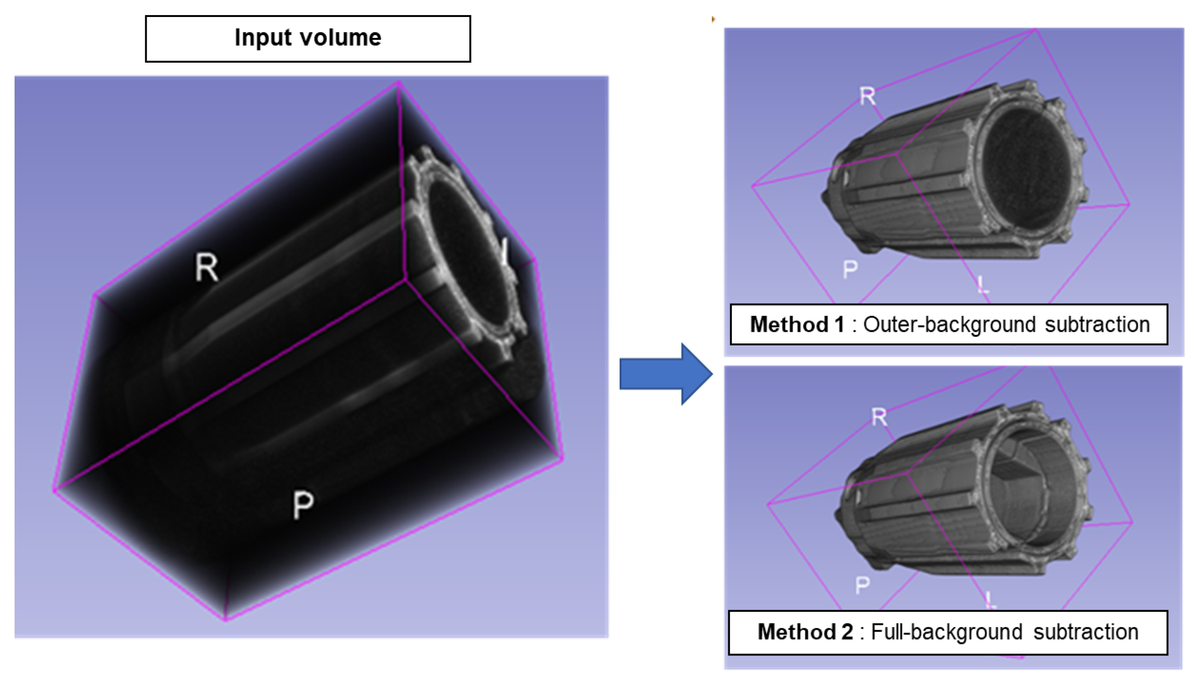
Then, the binary mask volume is used as a reference to extract only the tool data from the CT data. In this work, two different background subtractions were developed. The binary mask is overlayed over the input volume, and then the following are performed:
- Method 1 (outer-background subtraction): removes only the outer background to avoid removing critical ROIs from hollow object tools. The outer boundary pixels of the tool in the scanned volume are identified, and all pixels that fall outside the boundary pixels are removed. This methods is suitable for hollow tools;
- Method 2 (full-background subtraction): removes noisy data from both the inner and outer parts of the tools. All the pixels that are not overlapping with the binary mask are removed from the input volume. This methods is suitable for dense tools with small empty spaces.
Figure 10 shows an illustration of the two background subtraction methods. The input image has dark regions around and also inside the tool. First, the mask image is generated, then the background pixels are identified and removed. After removing those backgrounds, the top image is cleaned from both the inner and outer parts, and the lower image shows the output when only the outer noisy background is removed.
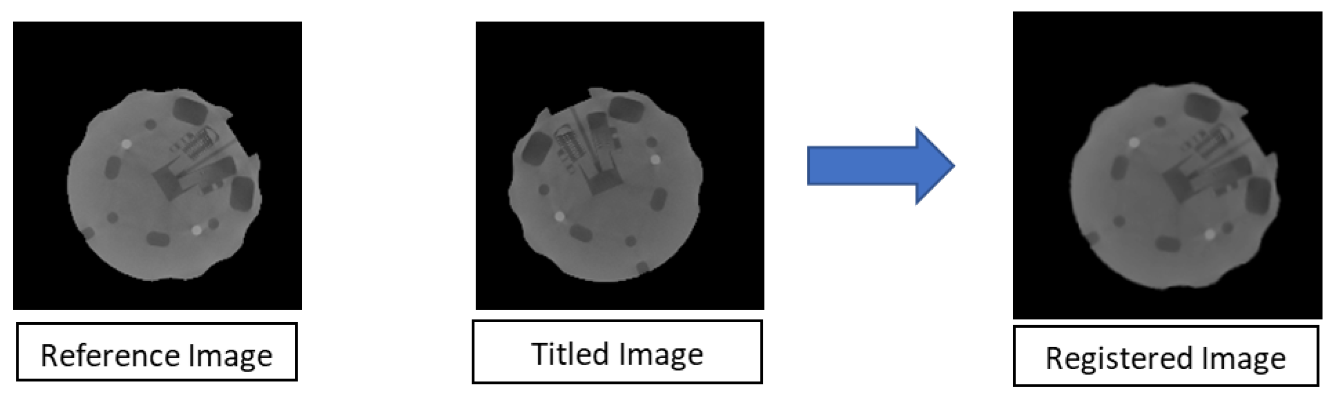
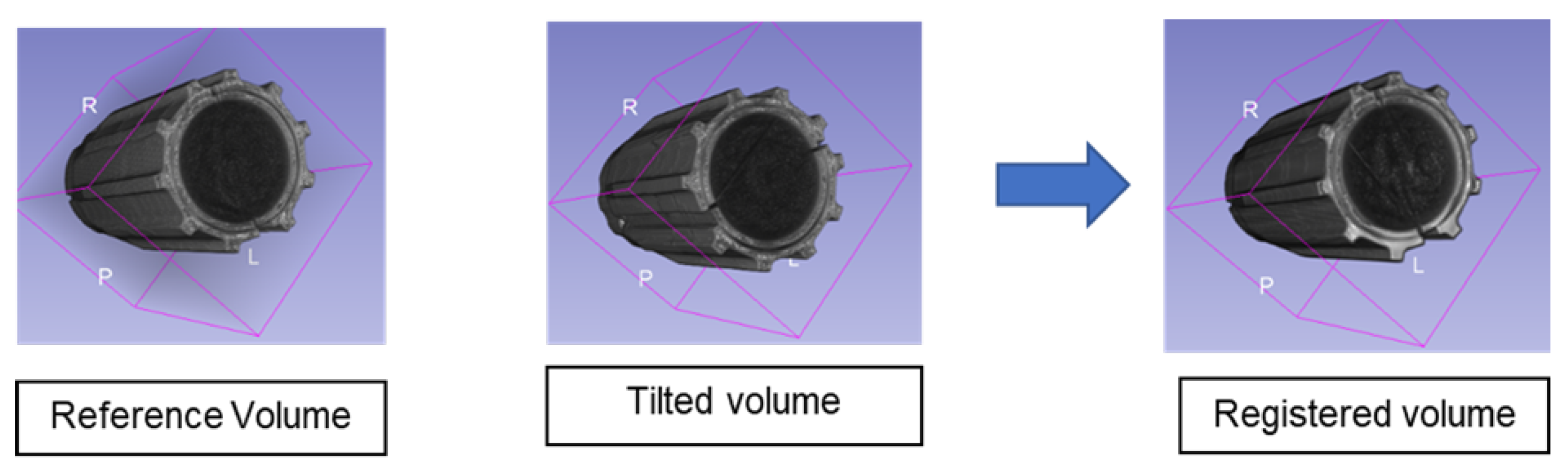
4.2. Registration
The registration function aligns the input image/volume according to the reference image/volume. This function was also developed using the DIPY library. The library function performs the translation, scaling, rotation, and affine translation operations to register 2D images or 3D volumes. There are a few parameters we need to set to register image or volume data using the DIPY library function:
- Reference_data: the image or volume data, according to which the input data will be registered;
- Input_data: the image or volume to be registered;
- Nbins: a value indicating the number of bins to compute the intensity histogram. The default value of 32 was used in this case;
- sampling_proportion: a value between zero and one, indicating the sampling ratio. A “None” value was used here to specify full sampling;
- level_iters: a sequence of numbers indicating the number of iteration per resolution. Three resolutions with iterations for 2D images and iterations for 3D volumes were specified in this case;
- Sigmas: a sequence of floats indicating the custom smoothing parameters. The default value of was used;
- Factors: sequence of floats indicating the custom scale factors. The default value of was used.
However, this library function alone cannot perform registration correctly. Therefore, an additional feature was developed to improve the DIPY library and fit our input CT data. In the proposed Toolbox, a new improvement denoted DIPY+ was implemented to improve the registration function so that it fit our real CT dataset based on the following features:
- Propose a new metric to access the registration performance to estimate the rotational angle between the scaled-down input and reference images/volumes;
- Improve the quality reduction and execution time by performing a single transformation using the estimated rotational angle and transformation factors, applied once to the original-sized images/volume instead of multiple small rotation steps using the default DIPY library.
4.3. Performance Analysis
Table 1 shows the performance of the different functions of the pre-processing data module on real CT datasets provided by our collaborators. There were four different combinations of methods with which we compared the results, as shown in Table 1.
The Peak Signal-to-Noise Ratio (PSNR) value was used to measure the performance. The obtained results showed that Method 1 and DIPY+ was the best combination to achieve a higher PSNR. In addition, with Method 2 (full-background subtraction with complete inner and outer noise removal), the lower density internal components of the tool were sometimes removed with noise. Thus, this method cannot be used for hollow tools with small internal components. It is worth mentioning that the DIPY library’s efficiency significantly decreased while dealing with the big rotational difference between the reference and input data.
Figure 13 shows an example of the introduced surface-level distortion due to the registration and the reduction in the volume resolution. It also demonstrates that the proposed DIPY+ performed better than the standard DIPY registration. Therefore, the proposed DIPY+ enhanced registration algorithm can solve the distortions related to the big volume size. However, this cannot be guaranteed for a huge volume size (greater than ), which needs to be processed in sub-volumes.
4.4. Limitations
The main limitations of the pre-processing module are presented as follows:
- Resizing the image or volume is required to meet the computational resources: memory and GPU speed. However, some small defects will become undetectable after scaling down the original volume;
- Registration will further affect the defects’ detection by smoothing the image/volume. This will introduce fake surface defects’ detection, of which we need to be aware.
5. Defect Inspection
Defect or fault inspection is performed in a hybrid framework integrating all the computer vision and deep-learning-based algorithms. Therefore, the final decision is derived from different detection phases (prediction, localization, and characterization) depending on the type of data and the availability of annotations. Figure 14 presents the defect inspection flowchart with the user and system interaction.
The main components of the defect inspections are presented in the following sections.
5.1. Defect Classification
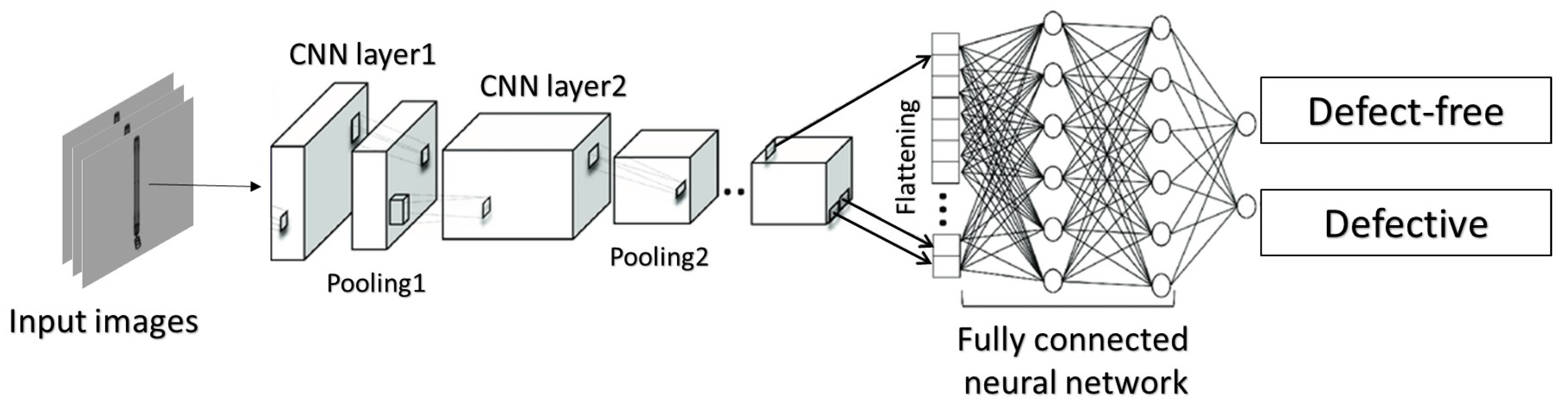
Defect prediction is the first step of the inspection where the scan is classified as defective or defect-free. Image classification research and applications are growing rapidly due to advances in Machine Learning (ML) and deep learning. In recent decades, many classification models, techniques, and frameworks have been presented. Some works focused on developing new frameworks to reduce spatial redundancy in image classification tasks, saving computational cost, memory footprint, and power consumption [39]. Wickramanayake et al. [40] introduced a framework, BetteR Accuracy from Concept-based Explanation (BRACE), to recognize candidate samples obtained from image repositories for data augmentation. Other works proposed new model architectures to deal with model scalability with high-resolution features such as the Global Filter Network (GFNet) [41]. Carter et al. [42] proposed a batched gradient SIS to find sufficient salient supporting input features/subsets in complex datasets. Some other works focused on missing labels and incomplete annotation, such as Hu et al. [43], who proposed a novel method named “one-bit supervision” for data annotation in image classification tasks with incomplete annotations. In the defect prediction/classification function, different state-of-the-art deep learning architectures are used as a backbone to perform binary classification of 2D images/3D volumes. Figure 15 shows the general framework of the architecture of defect prediction.
The input image needs some preparations and pre-processing such as resizing and data augmentation such as random rotation, horizontal and vertical flip, and color jitter. Figure 16 shows an illustration of the classification framework.
For instance, the classification framework uses the Resnet18-based model for binary classification. The performance of the trained model, for 200 epochs using real CT dataset, is shown in Figure 17.
On that note, during the data preparation, it was ensured that the class distribution of the dataset had a balanced number of images. Our contribution brings into light the application of existing deep learning architectures such as Resnet18 on industrial CT scans for image classification.
5.2. Defect Localization
The defect localization uses the image processing algorithm to localize the defect based on the residual image between the faulty image and the reference image (defect-free image). It is worth mentioning that the object might be noisy, tilted, or shifted. Thus, it is crucial to pre-process the images to ensure that the reference image has the maximum similarity to the faulty image. For 2D images, the defect localization is based on the analysis of the residual image and noise refinement to cancel the noise and neglect the non-relevant fault. The localization algorithm and flowcharts are presented in Figure 18 and Algorithm 1 respectively.
For a 3D volume, this same algorithm is extended to defect localization by applying it on every single slice of the volume. The output defect slices are concatenated, forming the final output 3D defect volume.

5.3. Fault Characterization
The defect characterization localizes the defect and recognizes its characteristics: type, location, and name of the defect (missing parts, broken parts):
- Defect location;
- Defect type: missing component, broken component;
- Name of the defective component;
- Additional statistics: defective volume ratio.
The defect characterization uses a labeled 3D volume of the tool to recognize and characterize the different defective components. The flowchart of the defect characterization is shown in Figure 20.
5.4. Limitations
The strength of the inspection module encompasses different factors and advanced features that can be summarized in two main points: First, build an automated full-inspection framework based on the combination of image processing and the deep learning technique contributing to the final inspection report and improving its accuracy. Second, use the inspection result, after expert validation, for further training of the learning models. This will build more generalizable and adaptive learning models with stable and trustworthy outcomes. However, there are still some limitations to be investigated in the future, such as:
- The module performance is highly dependent on the reprocessing module. Therefore, the obtained result becomes better with a good preparation and processing step: background subtraction and registration;
- The parameters of the defect detection algorithm are tuned to an optimal value for the data used. This parameter might slightly affect the performance when using new data.
6. Comparison to Some Existing Inspection Toolboxes
In terms of industrial applications, there exist some X-ray-CT-based software solutions on the market for CT visualization and inspection such as [26,27,28]. In addition, other products use hardware–software solutions for automated industrial processes such as the Carl Zeiss AG [29], the robotic inspection arm of VisiConsult X-ray Systems [30], CT inspection with automated tool-loading robotic arms [45], and robotic U-shaped inspection arms [46]. Table 2 shows a detailed comparison of the existing CT inspection systems and algorithms.
7. Conclusions and Future Work
This work explored a new computer-aided diagnosis toolbox, called CTIMS-Toolbox, for X-ray CT data inspection. The CTIMS-Toolbox is based on a hybrid framework integrating computer vision and deep-learning-based algorithms. It contains three main modules: the data management, pre-processing, and defect inspection modules. The toolbox allows the input CT scan data to obtain an automated inspection report based on three detection steps: prediction, localization, and characterization. It can incrementally learn from the user experience to generate annotated data that are used to train the deep learning models further and improve their performance. The latter helps build a valuable knowledge base that can help accelerate the inspection operation and provide preventive insights about the tool’s safety for future usage. However, the different CTIMS-Toolbox modules have some limitations related to the database management, especially for a big data size, the quality distortion after the pre-processing step, the long execution time, and the parameter tuning for the inspection module. These limitations can be further improved as follows:
Data management: While the design of the database can certainly be restructured, there is significant potential to completely redefine the database framework by using big-data-type structures, such as graph-based databases [47,48] or columnar databases [49].
Preprocessing module: The integrated background subtraction and registration are implemented and tested on scans of one tool’s data. In the future, when different tools and scanning machines will come into use, we will work on the automation of the pre-processing module by the adaptive parameter selection based on the input CT data. In addition, we will optimize the implementation to reduce the execution time and storage capacity.
Inspection module: We will focus on designing an adaptive selection of the inspection algorithm’s parameters to fit all kinds of variability in X-ray CT data. Thus, we will use a deep regression model to estimate the optimal input parameter based on the input data features: noise level, resolution, contrast, etc.
Finally, the proposed CTIMS-Toolbox can inspect 2D and 3D CT data and generate annotations based on the inspection results after validation by an expert. With a proper configuration of the scanner parameters, beam energy, and detector resolution, the proposed toolbox can be used for most materials such as metal, plastic, wood, etc.
Author Contributions
H.A.G. is the Principle Investigator, designed the idea of whole system automation process, and participated in the design of the functions, system integration, CT technology, and algorithm development and validation within the CTIMS-Toolbox. M.I.S. designed and implemented the database management of the toolbox. M.J.A.K. developed the 2D and 3D registration methods to pre-process the CT data. M.J.A.K. and A.C. designed and implemented the semi-automated 3D volume labeling and annotation. O.G.A. designed the binary classification module for defect classification. A.C. designed the DSP-based defect localization algorithm. A.C. and M.J.A.K. designed and implemented the fault characterization algorithm. A.C., M.J.A.K., M.I.S. and H.A.G. conceived of and designed the automated flowchart for the full inspection module. M.J.A.K., M.I.S., O.G.A., A.C. and H.A.G. wrote the paper. All authors have read and agreed to the published version of the manuscript.
Funding
This research was funded by Mitacs Grant Number 215457.
Institutional Review Board Statement
Not applicable.
Informed Consent Statement
Not applicable.
Data Availability Statement
The data presented in this study are available on request from the corresponding author.
Acknowledgments
This work was supported by New Vision Systems Canada Inc. (NVS) and Mitacs. The authors would like to thank the collaborators from Diondo and Fraunhover, Germany.
Conflicts of Interest
The authors declare that no competing interest exist.
Abbreviations
The following abbreviations are used in this manuscript:
| NDT | Non-Destructive Testing |
| CT | Computed Tomography |
| CTIMS | CT-Based Integrity Monitoring System |
| SQL | Full Structured Query Language |
| MySQL | Framework based on SQL |
| CANDU | Canada Deuterium Uranium |
| DSP | Digital Signal Processing |
| DNN | Deep Neural Network |
| CNN | Convolutional Neural Network |
References
- Natural Resources Canada. Ressources Naturelles Canada; Natural Resources Canada: Gatineau, QC, Canada, 2011. [CrossRef]
- Natural Resources Canada. Uranium and Nuclear Power Facts; Natural Resources Canada: Gatineau, QC, Canada, 2019.
- Torgerson, D.F.; Shalaby, B.A.; Pang, S. CANDU technology for Generation III+ and IV reactors. Nucl. Eng. Des. 2006, 236, 1565–1572. [Google Scholar] [CrossRef]
- Chauveau, D. Review of NDT and process monitoring techniques usable to produce high-quality parts by welding or additive manufacturing. Weld. World 2018, 62, 1097–1118. [Google Scholar] [CrossRef]
- Masoom, H.; Adve, R.S.; Cobbold, R.S. Target detection in diagnostic ultrasound: Evaluation of a method based on the CLEAN algorithm. Ultrasonics 2013, 53, 335–344. [Google Scholar] [CrossRef]
- Seeram, E. Computed Tomography-E-Book: Physical Principles, Clinical Applications, and Quality Control; Elsevier Health Sciences: Amsterdam, The Netherlands, 2015. [Google Scholar]
- Villarraga-Gómez, H. Seeing is believing: X-ray computed tomography for quality control. Qual. Mag. 2016, 55, 20–23. [Google Scholar]
- Kim, F.H.; Pintar, A.; Obaton, A.F.; Fox, J.; Tarr, J.; Donmez, A. Merging experiments and computer simulations in X-ray Computed Tomography probability of detection analysis of additive manufacturing flaws. NDT E Int. 2021, 119, 102416. [Google Scholar] [CrossRef]
- Nachtrab, F.; Weis, S.; Keßling, P.; Sukowski, F.; Haßler, U.; Fuchs, T.; Uhlmann, N.; Hanke, R. Quantitative material analysis by dual-energy computed tomography for industrial NDT applications. Nucl. Instrum. Methods Phys. Res. Sect. A Accel. Spectrom. Detect. Assoc. Equip. 2011, 633, S159–S162. [Google Scholar] [CrossRef]
- Venkatesh, E.; Elluru, S.V. Cone beam computed tomography: Basics and applications in dentistry. J. Istanb. Univ. Fac. Dent. 2017, 51, S102. [Google Scholar] [CrossRef]
- Korobkin, M.; White, E.; Kressel, H.; Moss, A.; Montagne, J. Computed tomography in the diagnosis of adrenal disease. Am. J. Roentgenol. 1979, 132, 231–238. [Google Scholar] [CrossRef]
- Ketcham, R.A.; Carlson, W.D. Acquisition, optimization and interpretation of X-ray computed tomographic imagery: Applications to the geosciences. Comput. Geosci. 2001, 27, 381–400. [Google Scholar] [CrossRef]
- Riis, N.A.; Frøsig, J.; Dong, Y.; Hansen, P.C. Limited-data X-ray CT for underwater pipeline inspection. Inverse Probl. 2018, 34, 34002. [Google Scholar] [CrossRef]
- Xu, J.; Zhao, Y.; Li, H.; Zhang, P. An image reconstruction model regularized by edge-preserving diffusion and smoothing for limited-angle computed tomography. Inverse Probl. 2019, 35, 85004. [Google Scholar] [CrossRef] [Green Version]
- Fang, L.; Wang, Z.; Chen, Z.; Jian, F.; Li, S.; He, H. 3D shape reconstruction of lumbar vertebra from two X-ray images and a CT model. IEEE/CAA J. Autom. Sin. 2020, 7, 1124–1133. [Google Scholar] [CrossRef]
- Szabo, I.; Sun, J.; Feng, G.; Kanfoud, J.; Gan, T.H.; Selcuk, C. Automated Defect Recognition as a Critical Element of a Three Dimensional X-ray Computed Tomography Imaging-Based Smart Non-Destructive Testing Technique in Additive Manufacturing of Near Net-Shape Parts. Appl. Sci. 2017, 7, 1156. [Google Scholar] [CrossRef] [Green Version]
- Zhao, X.; Rosen, D.W. Simulation study on evolutionary cycle to cycle time control of exposure controlled projection lithography. Rapid Prototyp. J. 2016, 22, 456–464. [Google Scholar] [CrossRef]
- Dong, G.; Marleau-Finley, J.; Zhao, Y.F. Investigation of electrochemical post-processing procedure for Ti-6Al-4V lattice structure manufactured by direct metal laser sintering (DMLS). Int. J. Adv. Manuf. Technol. 2019, 104, 3401–3417. [Google Scholar] [CrossRef]
- Akcay, S.; Breckon, T. Towards automatic threat detection: A survey of advances of deep learning within X-ray security imaging. Pattern Recognit. 2022, 122, 108245. [Google Scholar] [CrossRef]
- Muzahid, A.A.M.; Wan, W.; Sohel, F.; Wu, L.; Hou, L. CurveNet: Curvature-Based Multitask Learning Deep Networks for 3D Object Recognition. IEEE/CAA J. Autom. Sin. 2021, 8, 1177–1187. [Google Scholar] [CrossRef]
- Huang, Z.; Yang, S.; Zhou, M.C.; Gong, Z.; Abusorrah, A.; Lin, C.; Huang, Z. Making accurate object detection at the edge: Review and new approach. Artif. Intell. Rev. 2021, 1–30. [Google Scholar] [CrossRef]
- Mery, D.; Arteta, C. Automatic defect recognition in X-ray testing using computer vision. In Proceedings of the 2017 IEEE Winter Conference on Applications of Computer Vision, WACV 2017, Santa Rosa, CA, USA, 24–31 March 2017; Institute of Electrical and Electronics Engineers Inc.: Piscataway, NJ, USA, 2017; pp. 1026–1035. [Google Scholar] [CrossRef]
- Miao, C.; Xie, L.; Wan, F.; Su, C.; Liu, H.; Jiao, J.; Ye, Q. Sixray: A large-scale security inspection X-ray benchmark for prohibited item discovery in overlapping images. In Proceedings of the IEEE Computer Society Conference on Computer Vision and Pattern Recognition, Long Beach, CA, USA, 15–20 June 2019; pp. 2114–2123. [Google Scholar] [CrossRef] [Green Version]
- Gaus, Y.F.A.; Bhowmik, N.; Akcay, S.; Breckon, T. Evaluating the transferability and adversarial discrimination of convolutional neural networks for threat object detection and classification within X-ray security imagery. In Proceedings of the 18th IEEE International Conference on Machine Learning and Applications, ICMLA 2019, Boca Raton, FL, USA, 16–19 December 2019; pp. 420–425. [Google Scholar] [CrossRef] [Green Version]
- Tang, Z.; Tian, E.; Wang, Y.; Wang, L.; Yang, T. Nondestructive Defect Detection in Castings by Using Spatial Attention Bilinear Convolutional Neural Network. IEEE Trans. Ind. Inform. 2021, 17, 82–89. [Google Scholar] [CrossRef]
- Speed|Scan CT 64 | High-Speed CT Scanner. Available online: https://www.bakerhughesds.com/waygate-technologies/cases-speedscan-CT64 (accessed on 10 December 2021).
- Series Inspection CT | X-ray CT Systems | Nikon Metrology. Available online: https://www.nikonmetrology.com/en-us/x-ray-ct/x-ray-ct-systems-series-inspection-ct (accessed on 10 December 2021).
- YXLON-YXLON X-ray and CT Inspection Systems. Available online: https://www.yxlon.com/en/products/x-ray-and-ct-inspection-systems/yxlon-ux20 (accessed on 10 December 2021).
- Hashem, N.; Pryor, M.; Haas, D.; Hunter, J. Design of a Computed Tomography Automation Architecture. Appl. Sci. 2021, 11, 2858. [Google Scholar] [CrossRef]
- XRHRobotStar-In-Line ADR X-ray Inspection. Available online: https://visiconsult.de/products/ndt/xrhrobotstar/ (accessed on 10 December 2021).
- Letkowski, J. Doing database design with MySQL. J. Technol. Res. 2015, 6, 1. [Google Scholar]
- Bandaru, A. AMAZON WEB SERVICES. 2020. Available online: https://www.researchgate.net/profile/Avinash-Bandaru/publication/347442916_AMAZON_WEB_SERVICES/links/5fdc33dba6fdccdcb8d6dbe0/AMAZON-WEB-SERVICES.pdf (accessed on 10 December 2021).
- Al-Sayyed, R.M.; Hijawi, W.A.; Bashiti, A.M.; AlJarah, I.; Obeid, N.; Adwan, O.Y. An Investigation of Microsoft Azure and Amazon Web Services from Users’ Perspectives. Int. J. Emerg. Technol. Learn. 2019, 14, 217–241. [Google Scholar] [CrossRef] [Green Version]
- Kaushik, P.; Rao, A.M.; Singh, D.P.; Vashisht, S.; Gupta, S. Cloud Computing and Comparison based on Service and Performance between Amazon AWS, Microsoft Azure, and Google Cloud. In Proceedings of the 2021 International Conference on Technological Advancements and Innovations (ICTAI), Tashkent, Uzbekistan, 10–12 November 2021; IEEE: Piscataway, NJ, USA, 2021. [Google Scholar] [CrossRef]
- Brierley, N. Mapping Performance of CT. In Proceedings of the International Symposium on Digital Industrial Radiology and Computed Tomography, Fürth, Germany, 2–4 July 2019. [Google Scholar]
- Feldkamp, L.A.; Davis, L.C.; Kress, J.W. Practical cone-beam algorithm. J. Opt. Soc. Am. A 1984, 1, 612. [Google Scholar] [CrossRef] [Green Version]
- Lei, Y.; Fu, Y.; Wang, T.; Liu, Y.; Patel, P.; Curran, W.J.; Liu, T.; Yang, X. 4D-CT deformable image registration using multiscale unsupervised deep learning. Phys. Med. Biol. 2020, 65, 085003. [Google Scholar] [CrossRef] [PubMed]
- Garyfallidis, E.; Brett, M.; Amirbekian, B.; Rokem, A.; van der Walt, S.; Descoteaux, M.; Nimmo-Smith, I. Dipy, a library for the analysis of diffusion MRI data. Front. Neuroinform. 2014, 8, 8. [Google Scholar] [CrossRef] [Green Version]
- Wang, Y.; Lv, K.; Huang, R.; Song, S.; Yang, L.; Huang, G. Glance and Focus: A Dynamic Approach to Reducing Spatial Redundancy in Image Classification. In Advances in Neural Information Processing Systems; Larochelle, H., Ranzato, M., Hadsell, R., Balcan, M.F., Lin, H., Eds.; Curran Associates, Inc.: Red Hook, NY, USA, 2020; Volume 33, pp. 2432–2444. [Google Scholar]
- Wickramanayake, S.; Hsu, W.; Lee, M.L. Explanation-based Data Augmentation for Image Classification. In Proceedings of the Thirty-Fifth Conference on Neural Information Processing Systems, Virtual, 6–14 December 2021. [Google Scholar]
- Rao, Y.; Zhao, W.; Zhu, Z.; Lu, J.; Zhou, J. Global Filter Networks for Image Classification. arXiv 2021, arXiv:2107.00645. [Google Scholar]
- Carter, B.; Jain, S.; Mueller, J.; Gifford, D.K. Overinterpretation reveals image classification model pathologies. arXiv 2020, arXiv:2003.08907. [Google Scholar]
- Hu, H.; Xie, L.; Du, Z.; Hong, R.; Tian, Q. One-bit Supervision for Image Classification. In Proceedings of the Advances in Neural Information Processing Systems 33: Annual Conference on Neural Information Processing Systems 2020, NeurIPS 2020, Virtual, 6–12 December 2020. [Google Scholar]
- Haralick, R.M.; Sternberg, S.R.; Zhuang, X. Image Analysis Using Mathematical Morphology. IEEE Trans. Pattern Anal. Mach. Intell. 1987, PAMI-9, 532–550. [Google Scholar] [CrossRef]
- Clarke, A.L.; Vieyra, M.; Nicholson, P.I.; Szabo, I.; Logeswaran, G.; Kappatos, V.; Selcuk, C.; Gan, T.H. Development of an automated digital radiography system for the non-destructive inspection of green powder metallurgy parts. In Proceedings of the Euro PM 2014 International Conference and Exhibition. European Powder Metallurgy Association (EPMA), Salzburg, Austria, 21–24 September 2014. [Google Scholar]
- Krumm, M.; Sauerwein, C.; Hämmerle, V.; Heile, S.; Schön, T.; Jung, A.; Sindel, M. Rapid Robotic X-ray Computed Tomography of Large Assemblies in Automotive Production. In Proceedings of the 8th Conference on Industrial Computed Tomography, (iCT 2018), Wels, Austria, 6–9 February 2018; Number iCT. pp. 1–9. [Google Scholar]
- Yoon, B.H.; Kim, S.K.; Kim, S.Y. Use of graph database for the integration of heterogeneous biological data. Genom. Inform. 2017, 15, 19. [Google Scholar] [CrossRef] [Green Version]
- Paredaens, J.; Peelman, P.; Tanca, L. G-Log: A graph-based query language. IEEE Trans. Knowl. Data Eng. 1995, 7, 436–453. [Google Scholar] [CrossRef]
- Plattner, H. The impact of columnar in-memory databases on enterprise systems: Implications of eliminating transaction-maintained aggregates. Proc. VLDB Endow. 2014, 7, 1722–1729. [Google Scholar] [CrossRef] [Green Version]
Figure 1.
The framework of the CT data inspection using the proposed CTIMS-Toolbox.

Figure 2.
The user interface of the proposed CTIMS-Toolbox.

Figure 3.
The general flowchart of the CTIMS-Toolbox.

Figure 4.
The database management flowchart.

Figure 5.
Example of a folder structure: (a) input tool named train_tool; (b) output results’ structure.
Figure 5.
Example of a folder structure: (a) input tool named train_tool; (b) output results’ structure.

Figure 6.
Database tables’ structure diagram.

Figure 7.
Flowchart of incremental model training.

Figure 8.
The data flow cycle from loading to applying inspection, till the storage of the results.

Figure 9.
The general workflow of the pre-processing module.

Figure 10.
Illustration of the 3D background subtraction.

Figure 11.
Example of 2D image registration.

Figure 12.
Example of 3D volume registration.

Figure 13.
Example of quality reduction due to registration. With outer-background subtraction and using DIPY+ (top) and using DIPY (bottom).
Figure 13.
Example of quality reduction due to registration. With outer-background subtraction and using DIPY+ (top) and using DIPY (bottom).

Figure 14.
The full inspection flowchart in the CTIMS-Toolbox.

Figure 15.
Example of the general framework of Convolutional-Neural-Network (CNN)-based binary classification.
Figure 15.
Example of the general framework of Convolutional-Neural-Network (CNN)-based binary classification.

Figure 16.
The classification framework with data augmentation.

Figure 17.
Example of the training/validation loss and accuracy of the ResNET18 classification model.
Figure 17.
Example of the training/validation loss and accuracy of the ResNET18 classification model.

Figure 18.
The DSP-based defect localization flowchart.

Figure 19.
Example of defect categorization.

Figure 20.
The defect characterization flowchart.


Table 1.
Performance analysis of the pre-processing module.
| Dataset | Background Subtraction | Registration | PSNR (dB) | Execution Time (s) |
|---|---|---|---|---|
| Real CT data | Outerbackground removal | DIPY | 25.77 | 357 6 min |
| DIPY+ | 37.71 | 1112 ∼18.5 min | ||
| Volume size 113 × 166 × 113 | Full-background removal | DIPY | 24.62 | 341 ∼5.7 min |
| DIPY+ | 35.13 | 1095 ∼18.3 min |
Table 2.
Comparison of existing CT inspection algorithms and systems.
| System | Defect Localization | Commercialized | Remarks | |
|---|---|---|---|---|
| DSP | DNN | |||
| DIRA-GREEN [45] | ✓ | DIRA-GREEN https://www.youtube.com/watch?v=69asRG8mN7Q (accessed on 10 December 2021) | + automated system − only for small-sized tools | |
| Automated Defect Recognition (ADR) [16] | ✓ | qualinet www.qualinet-project.com (accessed on 10 December 2021) | + different defect location images are used as the “golden” image to compare with − only valid for one unique tool of known shape and defect locations | |
| RoboTom [46] | ? | ? | RaySCAN https://www.rayscan.eu/InnovativeTechnik_e.html (accessed on 10 December 2021) | + inspect large assembly joints − focuses on porosity in weld defects |
| ADR X-ray inspection [30] | ? | ? | XRHRobotStar https://visiconsult.de/products/ndt/xrhrobotstar/ (accessed on 10 December 2021) | + small and medium parts’ inspection + Part recognition − focuses on porosity in weld defects |
| CTIMS-Toolbox | ✓ | ✓ | (not yet) | + small and medium parts’ inspection + CT data annotation − validated only for metallic materials |
Publisher’s Note: MDPI stays neutral with regard to jurisdictional claims in published maps and institutional affiliations. |
© 2022 by the authors. Licensee MDPI, Basel, Switzerland. This article is an open access article distributed under the terms and conditions of the Creative Commons Attribution (CC BY) license (https://creativecommons.org/licenses/by/4.0/).
Share and Cite
MDPI and ACS Style
Gabbar, H.A.; Chahid, A.; Khan, M.J.A.; Adegboro, O.G.; Samson, M.I. CTIMS: Automated Defect Detection Framework Using Computed Tomography. Appl. Sci. 2022, 12, 2175. https://0-doi-org.brum.beds.ac.uk/10.3390/app12042175
AMA Style
Gabbar HA, Chahid A, Khan MJA, Adegboro OG, Samson MI. CTIMS: Automated Defect Detection Framework Using Computed Tomography. Applied Sciences. 2022; 12(4):2175. https://0-doi-org.brum.beds.ac.uk/10.3390/app12042175
Chicago/Turabian StyleGabbar, Hossam A., Abderrazak Chahid, Md. Jamiul Alam Khan, Oluwabukola Grace Adegboro, and Matthew Immanuel Samson. 2022. "CTIMS: Automated Defect Detection Framework Using Computed Tomography" Applied Sciences 12, no. 4: 2175. https://0-doi-org.brum.beds.ac.uk/10.3390/app12042175
Note that from the first issue of 2016, this journal uses article numbers instead of page numbers. See further details here.