
Pay Zone Determination Using Enhanced Workflow and Neural Network


1
Department of Geosciences, Universiti Teknologi PETRONAS, Bandar Seri Iskandar, Perak 32610, Malaysia
2
Osaimi Engineering Office, Al-Khobar 35717, Saudi Arabia
*
Authors to whom correspondence should be addressed.
Appl. Sci. 2022, 12(4), 2234; https://0-doi-org.brum.beds.ac.uk/10.3390/app12042234
Submission received: 5 January 2022
/
Revised: 19 January 2022
/
Accepted: 20 January 2022
/
Published: 21 February 2022
(This article belongs to the Special Issue Artificial Intelligence Applications in Petroleum Exploration and Production)
Abstract
:Featured Application
This article demonstrates the use of a type of unsupervised learning named self-organizing maps to delineate hydrocarbons.
Abstract
Amplitude versus offset (AVO) analysis and attributes are frequently utilized during the early stages of exploration when no well has been drilled. However, there are still some drawbacks to this method, including the fact that it involves a substantial amount of time and experience, as well as the subjectivity of manual analysis. By utilizing unsupervised learning, this process can be done more objectively and faster. Unsupervised learning can detect anomalies and identify patterns to understand more about the datasets since, at this early stage of exploration, there is still a lack of information and labelling. A type of unsupervised learning referred to as self-organizing maps (SOM) is applied in this study to delineate hydrocarbons from given AVO properties that were used to detect hydrocarbons. SOM is also used to eliminate redundancy in the selection of attributes prior to the delineation procedure. The investigation began with well log data and progressed ahead into multiple fluid conditions to evaluate the model’s ability to identify hydrocarbons. The analysis can then be extended to the seismic dataset. By combining SOM, correlation coefficient, and mean–median, a method is devised for filtering features to remove redundancy. On the hydrocarbon delineation process, the model managed to detect hydrocarbons using well log simulations and was confirmed using water saturation logs. Additionally, the model is validated using real seismic data, demonstrating a promising performance in defining probable hydrocarbons. The proposed method enables early detection of hydrocarbon content during the preliminary stage of exploration when no well is accessible.
1. Introduction
A pay zone is a section of a reservoir that contains economically recoverable hydrocarbons. Finding the pay zone is critical for determining the optimal position of the production well. These can help to mitigate the uncertainty and risk associated with drilling a new well. However, pay zone determination is often carried out at the well log scale using petrophysical analysis. Meanwhile, only seismic data are available during the early stages of investigation.
A direct hydrocarbon indicator (DHI) is a high-amplitude seismic response anomaly generated by the presence of hydrocarbons [1]. These phenomena occur because of the presence of gas, which is significantly more compressible than brine and, hence, decreases its bulk modulus. DHI responses are most frequently observed in gas saturated sand; however, oil can also exhibit DHI responses. The high amplitude is often triggered by a quick decrease in impedance. However, the presence of hydrocarbons does not always impact DHI anomalies. To determine the presence of DHI, AVO analysis and characteristics are typically used. Nonetheless, there are various difficulties associated with these DHI assessments, one of which is that low gas saturation typically exhibits equivalent reactions to high saturation gas [2]. Additionally, this procedure demands considerable effort and experience, not to mention the subjectivity of the analysis.
Unsupervised learning has been commonly used in the geoscience field of research in recent years because of its ability to find new patterns and information from the combination of features, which is typically met with unlabeled data problems. This method may be used as a substitute or a solution in the absence of prior information to identify the pay zone during the pre-drilling exploration phase. Unsupervised learning approaches are being used in geoscience to assist AVO cross-plotting in characterizing its background trend [3]. Another example is that unsupervised learning can make recommendations about which attributes to use in multi-attribute analysis [4,5]. Unsupervised learning can also be utilized to detect the geological depositional environment [6,7].
Since there is still a lack of labelling and prior information in the early stage of exploration, applying unsupervised learning would be suitable as an early detection technique to detect the presence of hydrocarbons when no well is accessible. Where supervised machine learning needs labels to train the model, unsupervised machine learning does not need labels to train the model. Unsupervised learning allows us to identify unrecognizable patterns and detect anomalies, providing more understanding through the datasets. The model may be able to reduce the amount of time required for the analysis or interpretation that is typically performed by humans by combining the available AVO features to provide more objective analysis to assist in seismic interpretation and zone delineation [8,9].
This research provides an alternative way of delineating hydrocarbons from a conventional method, where several AVO attributes are being analyzed independently and manually. This will result in potential subjectivity and bias in the analysis. Meanwhile, by using our proposed method, the SOM selected and combined several AVO attributes and specified to delineate specific clusters, and, in this research, it is the anomaly of the AVO attributes that is related to the indication of hydrocarbons.
This research’s workflow can be utilized for other potential anomaly detection problems. For example, it can be applied to detect the overpressure zone before drilling by using multiple seismic attributes [10]. Other potential research on detecting the leakage of CO2 storage monitoring from seismic data can also be done by using this workflow [11].
2. AVO Attributes
AVO attributes are attributes that are derived from pre-stack seismic data that are calculated through AVO equation analysis. The following is the written form of Equation (1):
where
A is referred to as the intercept, B is the gradient, and C is the curvature term. If the third term (curvature) is removed, then:
Then, it can be turned into matrix and A and B are obtained through over-determined inversion as follows:
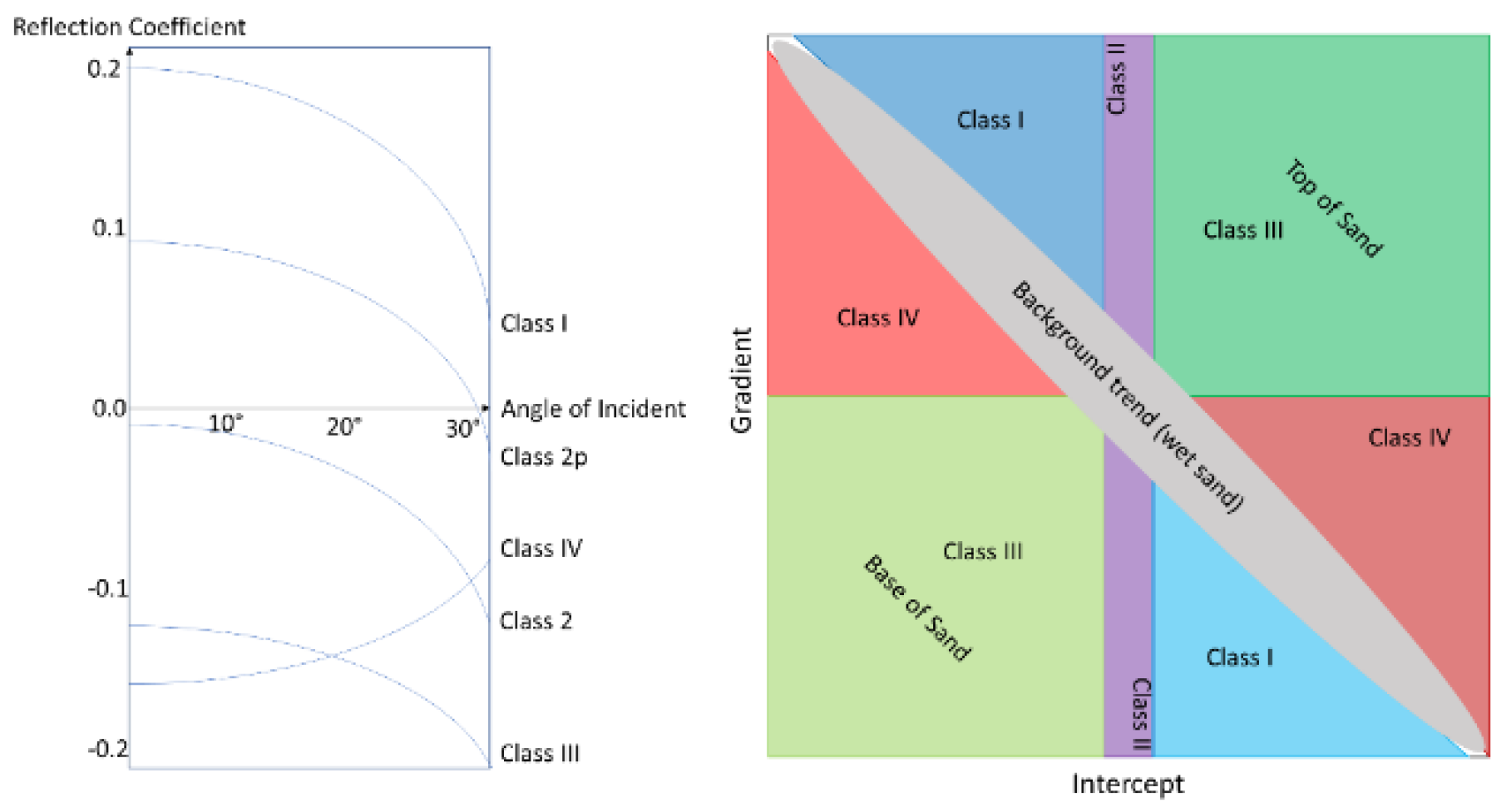
Generally, AVO cross-plotting is being conducted to perform the analysis where intercept and gradient are defined as the X and Y axis. From the cross-plotting technique, it can also be used to classify AVO response to the gas saturated reservoir (see Figure 1).
Numerous AVO attributes are derived from the combination of intercept and gradient; some of them are dot product of intercept and gradient. For positive intercept value condition examples, as the angle of incident increases, the product is negative if the amplitude is decreasing and positive if the amplitude is increasing and vice versa. This method could produce a positive value to the class 3 AVO anomalies and strengthen the indication of it [12]. The statement can be explained further in the Equation (3) below:
This Equation (3) can be further elaborated by utilizing sign function that extracts the property of value of intercept or gradient attributes whether positive, negative, or zero. The sign function is defined as follows:
Then, it is applied to product attributes as follows:
t can also be used to create scaled Poisson’s ratio change where it could give a better sight to class 2 AVO anomalies. The attributes can also be expected to show a decreasing value into a reservoir zone and increasing value into a water filled porosity zone [12]. Equation (5) is expressed as follows:
From the Aki–Richards Equation, scaled S-wave reflectivity can also be derived by assuming that Vp/Vs = 2 at intermediate angles (0° < θ < 30°). The Equation (6) is expressed as follows:
where A can be defined as (p-wave reflectivity).
If Vs/Vp = 0.5, then:
, if and then,
These p-wave and s-wave reflectivity values can also be used to generate a fluid factor that can be utilized to separate gas-associated reflector from background trend (brine sand/shale) interfaces. Equation (8) is expressed as follows: ; if Vp/Vs = 2, then
Currently, there is also a new and improved attribute from quality factor of compressional (P) wave (Qp) and shear wave (Qs) named scale of quality factor of P-wave (SQp) and scale of quality factor of S-wave (SQs). These attributes are utilized to discriminate lithology and hydrocarbon prediction [13,14]. Initially, SQp and SQs were formulated by utilizing bulk and shear modulus and crack density until recently; it has been improved that they can be derived from the intercept and gradient to get more sensitive AVO attributes [15]. Equations (10) and (11) are expressed as follows:
There are AVO attributes that can be generated from the angle stack itself, such as far-minus-near times far (FNXF), which is calculated by taking the change of amplitudes between near angle stack and far angle stack and multiplying it with far angle stack. The attribute is defined as follows:
3. Unsupervised Learning
Unsupervised learning is a machine learning algorithm that is used to analyze the natural pattern on the dataset where it would not need a training label during the progress. Several utilizations of unsupervised learning are clustering, dimensionality reduction, and anomaly detection. In the geosciences field of study, unsupervised learning has been applied to aid interpretation, such as multi-attribute analysis [6,7,8,16], AVO cross-plotting, and classification [3,17].
3.1. Self-Organizing Maps
Self-organizing maps (SOM) is a type of unsupervised learning algorithm that is also referred to as Kohonen maps. The key notion behind how SOM works is that it transforms multi-dimensional datasets into a typically non-linear two-dimensional representation in the form of a grid or map [18,19].
Self-organizing maps learn by matching the input datasets into the best nodes, and the nodes will be associated with other nodes that have a similar characteristic for a better fitting [19]. Initially, each input data sample or point will assign random weights to each node at first iteration. The weights are either the point representative or the coordinates of the input data sample and are used to determine the best node that fits with the data point. Euclidean distances between the input and the nodes are calculated to determine the best matching unit (BMU). The node with the shortest distance to the specific data point will be defined as the best matching unit. The weights inside the node will be updated to ensure a better match with the data point. The neighboring nodes will also be updated so that the nearby nodes will have a closer characteristic to the best matching unit node. As a result, the more identical nodes will be situated nearer to the grid. Meanwhile, the less identical will be located further away from the grid.
3.2. Mean–Median
Mean–median (MM) is an approach for filtering features that was proposed in this paper. It is a dispersion measure in which the absolute difference between the mean and median of the features is calculated. The higher the values, the more discriminatory power they have [20].
4. Dataset and Methodology
4.1. Dataset
The dataset used in this research is comprised of well log and seismic partial-stack data from the “X” field for model input. Three well logs, labeled A-1, A-2, and A-3, were used in this research. A-1 and A-2 are used to evaluate the model’s performance in synthetic seismic analysis, whereas A-3 is utilized to validate the model’s performance in real seismic analysis. This research makes use of partial stacks of seismic data. The partial stack is divided into near (05–15 degrees), mid (15–25 degrees), and far stacks (25–40 degrees) and covers an area of up to 185,000,000 m2. All datasets are obtained from Centre for Subsurface Imaging (CSI) Universiti Teknologi PETRONAS internal report.
4.2. Methodology
Fluid replacement modelling was used to prepare the dataset for hydrocarbon delineation simulation. A model’s performance on various hydrocarbon fluid conditions must be evaluated. Analyze the performance of each AVO attribute to differentiate hydrocarbon later. Gassmann’s equation for fluid substitution is used to describe fluid replacement if the ultimate fluid state is 80/20 oil/water or 80/20 gas/water where the initial fluid condition is 100% water. To extract AVO attributes from datasets created using fluid replacement modelling, click here. First, use Equation (1) to determine intercept and gradient using P-wave velocity log (Vp log), S-wave velocity log (Vs log), and density log. Other AVO properties can be generated using Intercept and Gradient after they have been constructed. There are also SQp and SQs. First, we need to generate near and far reflectivity using Equation (1), with near at 10° and far at 35°. This allows us to calculate FNXF characteristics using Equation (12). Finally, the AVO attributes must be wavelet convolved to simulate seismic conditions. Convolution is performed using ricker wavelet in this study.
The next step is to analyze feature selection. Prior to hydrocarbon delineation, selecting relevant AVO features is an important process. This step reduces the number of attributes that offer the same information to the anomaly detection process. The model can produce a 2D features map for each attribute using self-organizing maps. The feature map shows where the associated variables are high or low. The similarity of the feature maps indicates substantial interdependence [21]. To measure it quantitatively, a heatmap correlation analysis measures the correlation between produced attributes. The higher the correlation, the more redundant the traits are. The mean–median approach is used to choose the best features for further study. Mean–median is used to examine attribute dispersion. That is, the higher the dispersion, the better the abnormality may be identified. The attributes with the biggest dispersion will be used for further study, while the other can be omitted to reduce computational time on delineating hydrocarbon.
After selecting the attributes, hydrocarbon delineation is performed. Before applying the model to seismic scale, the analysis is performed at well log scale. In this case, self-organizing maps are used. The presence of hydrocarbon discovered by AVO characteristics is considered anomalous in this study. Quantization error is used as a statistical measure to discover anomalies using self-organizing maps. Quantization error is the distance between data samples and its best matching units. Meaning the quantization error increases as the distance between a data sample and the dataset’s overall distribution increase, causing it to be flagged as anomalous. The hydrocarbon delineation using self-organizing maps began with the training datasets. The datasets must be standardized before use to ensure that each attribute contributes equally to identifying hydrocarbon. Then the self-organizing maps model training can begin. It calculates quantization error for each data sample. Next, an error threshold is specified, and any data sample with a quantization error greater than the threshold is considered an anomaly. For this purpose, local minima of the quantization error distribution are computed. In this research, the model recognizing the data sample is an anomaly or a hydrocarbon. Because this is unsupervised learning, it is difficult to analyze model performance since there is no label to train the model. Instead, for this research, water saturation log is utilized to examine model performance to detect hydrocarbons. Those data samples with water saturation values less than 0.5 are labelled as hydrocarbons, while those with water saturation values equal to or more than 0.5 are labelled as not Hydrocarbons. If the outcome is satisfactory, the analysis can be moved to real seismic data. If not, hyperparameter tuning is required until the desired result is achieved.
Prior to conducting seismic scale analysis, seismic well tie and horizon picking should be performed to ensure the data reliability for analysis and validation. Seismic-well tie is being done to utilize well log as the confirmation of the presence of hydrocarbon in specific area. Horizon picking is being done to highlight our interest area which is “Top I-35”. This horizon will also be used to validate the presence of hydrocarbon. Types of AVO attributes used for hydrocarbon delineation in seismic scale will still be using the same configuration from the previous AVO attributes selection in well log scale. Then, hydrocarbon delineation is performed using SOM to detect potential hydrocarbon. To validate the result, the delineated hydrocarbon is compared with water saturation well log data. The model is also being analyzed in horizon map view to analyze the overall distribution of potential hydrocarbon in specific horizon.
In this research, Python programming language is used to conduct majority of the analysis started from dataset preparation, features selection, and application of SOM. RokDoc is used to perform fluid replacement modelling. Hampson/Russel Geoview is used to perform seismic-well tie, horizon picking analysis and delineating hydrocarbon using conventional method. Lastly, Petrel is used to aid seismic dataset preparation.
5. Results and Discussion
This part presents the results and the subsequent discussion, which were obtained from this research output. The analysis started from the well log scale, then continued to seismic scale. The analysis started at the synthetic well dataset to test the efficacy of the proposed workflow, followed by the testing on well data of well A-1 and A-2 in field “X”. Then, the analysis was finished by testing the model on seismic data from field “X”.
The results begin from the unsupervised learning analysis at the well log scale. The analysis was started from performing fluid replacement modelling first to create a simulation of an oil and gas reservoir. Then, several AVO attributes were extracted to be used as the inputs for the unsupervised learning model. In this part, AVO attributes can also be analyzed by determining the capability to distinguish hydrocarbons from brine qualitatively.
The unsupervised learning analysis was started by performing features selection to identify which features are best to be used as inputs, and then the process proceeded to the anomaly detection. In this research, self-organizing maps combined with mean–median and heatmap correlation was used to perform features selection to select the AVO attributes to reduce the redundancy.
Then, the performance of the hydrocarbon delineation was analyzed using self-organizing maps. The delineation result was validated with water saturation well log. The model was evaluated based on its accuracy in delineating hydrocarbons.
After the desired result was obtained at the well log scale, the analysis was shifted to the seismic scale, where the SOM algorithm was applied to delineate the potential hydrocarbons in seismic data using AVO attributes that were selected in the previous workflow. Before the SOM is applied, well log correlation and horizon picking need to be completed for the result validation and input preparation. The result will be shown in seismic section and horizon map slice to show the prediction result distribution and validated with the water saturation well log data that have been tied with seismic data.
5.1. Fluid Replacement Modelling and AVO Attributes Extraction
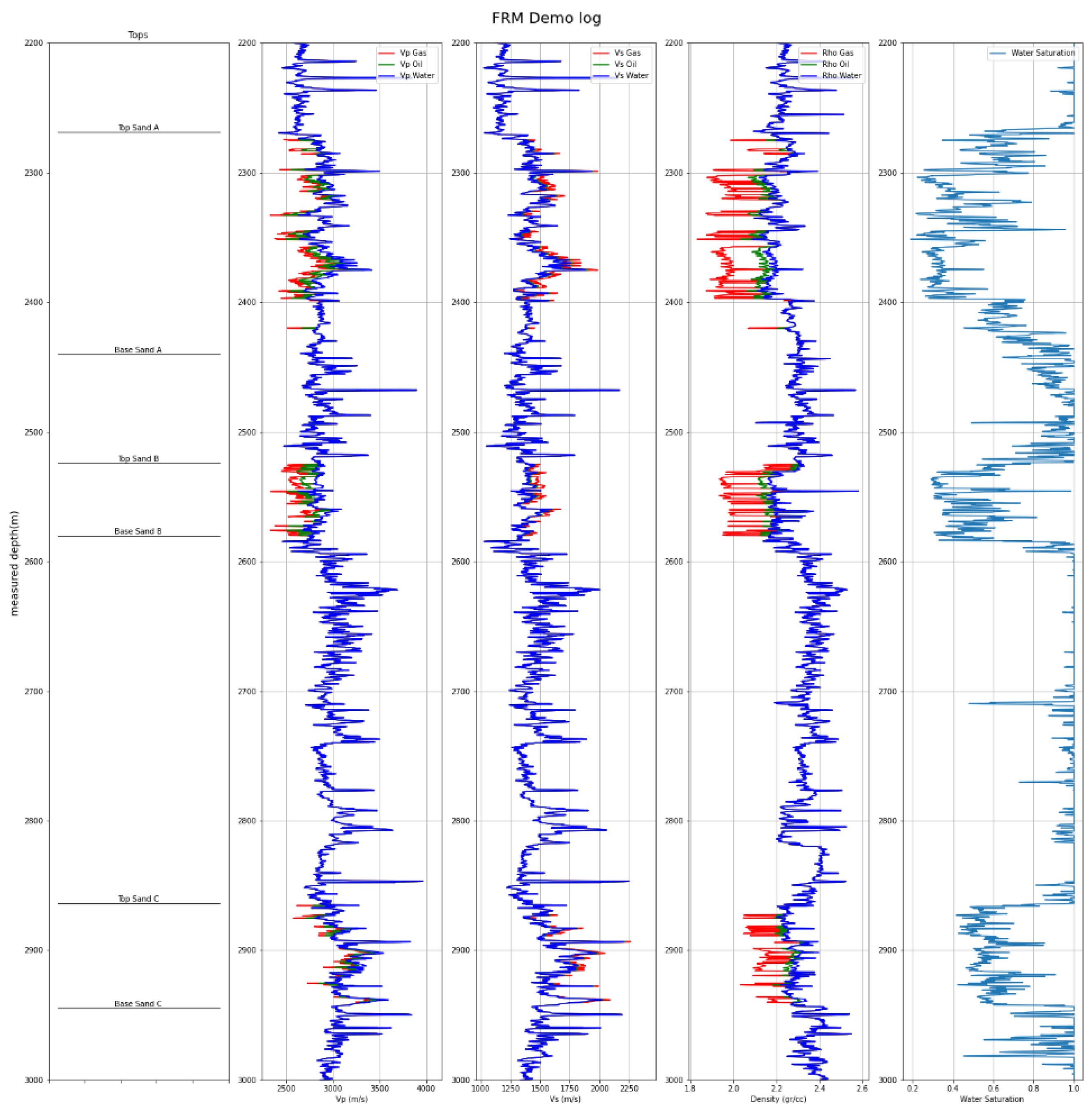
Fluid replacement modelling needs to be done to analyze the AVO attributes response through fluid changes. Gassmann’s equation for fluid substitution is used to perform fluid replacement modelling where the initial fluid was 100% water into two final fluid situations, 80% oil, 20% water, and 80% gas, 20% water (see Figure 2).
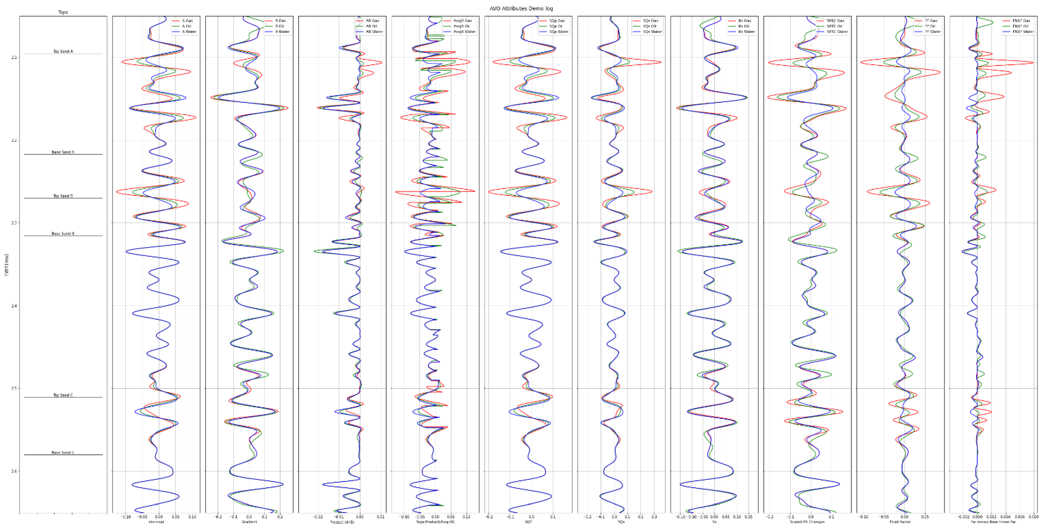
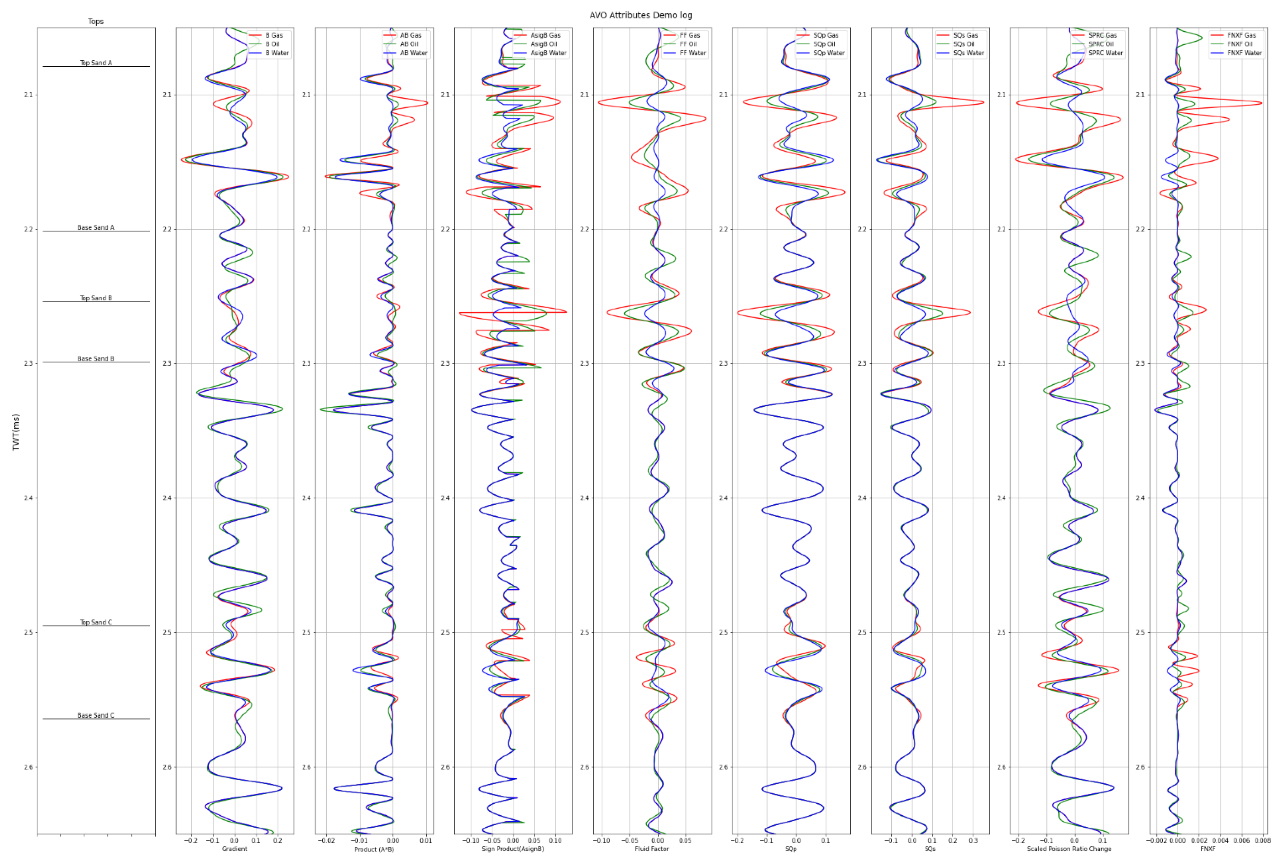
After the FRM model is created, the AVO attributes extraction can be conducted. The process started by calculating the intercept and gradient using Equation (2). From there, several AVO attributes can be derived, such as: product, sign of product, fluid factor, scaled Poisson ratio change, shear reflectivity, far minus near times far, SQp, and SQs (see Figure 3).
From the figure above, there is an attribute that could not differentiate between brine and hydrocarbons well: shear reflectivity. There are also several AVO attributes that can differentiate hydrocarbons very well such as: SQp, SQs, fluid factor, product. From this workflow feature, selection can be started by analyzing which AVO attributes will be appropriate to delineate hydrocarbon visually. For example, shear reflectivity can be excluded for further analysis.
5.2. Features Selection and Anomaly Detction Using Self-Organizing Maps at Well Data with Different Fluid Conditions
In this part, self-organizing maps (SOM) is used to conduct features selection to select the best AVO attributes for hydrocarbon delineation and anomaly detection to determine at which depth the hydrocarbon is identified. Feature selection is completed by analyzing the 2D distribution maps for each feature generated from the SOM algorithm (see Figure 4).
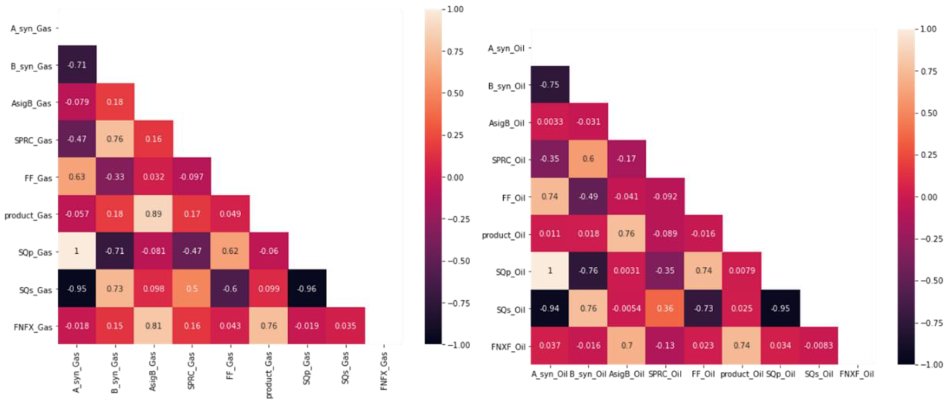
From the Figure 4, a distribution map is generated for each feature in the datasets. Each SOM feature map visualizes the area where the corresponding variables show high or low values. The similarities between the feature maps indicate that the features are strongly dependent on each other [21]. For example, the features map of SQp and intercept present the same distribution map. Therefore, having both to be used as inputs is redundant. Heatmap correlation is used to analyze the correlation between the feature maps quantitatively (see Figure 5). It is demonstrated by the correlation coefficient of the SOM feature map in Figure 5 that SQp and intercept have a high correlation between them.
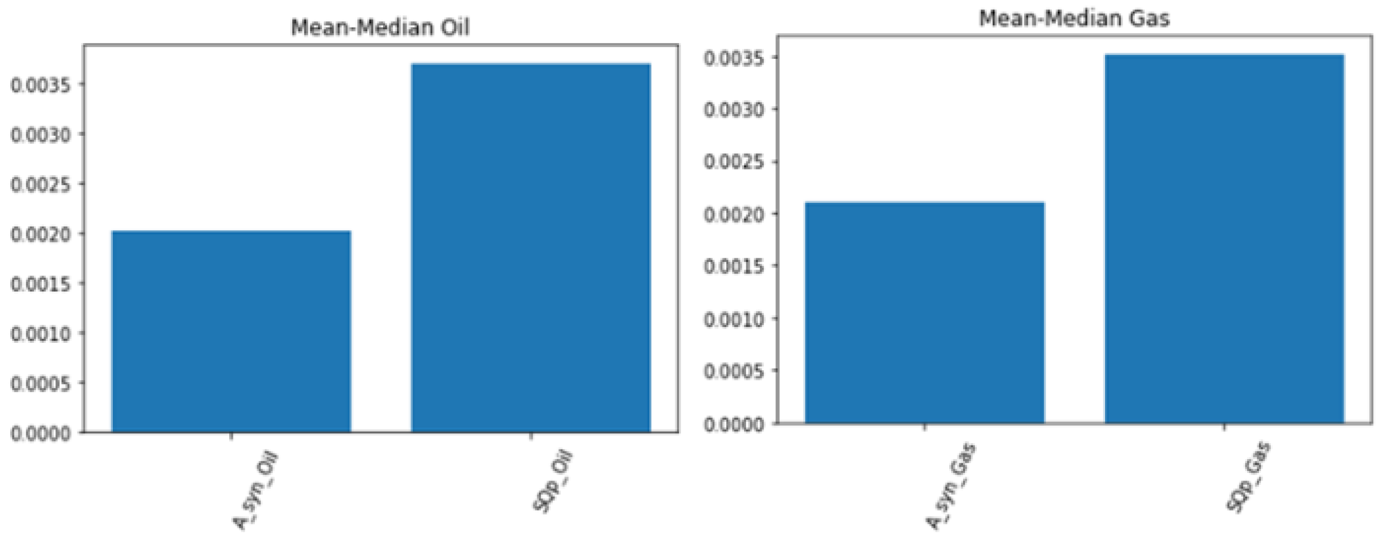
Hence, more features selection methods need to be conducted. In this research, the mean–median score is being applied due to its efficiency and being faster than embedded methods [20]. In this study, the mean–median score between the intercept and SQp attributes were calculated in two different fluid conditions and the highest score will be appointed as selected features (see Figure 6).
From Figure 6, it can be determined that the mean–median score of SQp in the oil and gas condition is higher than the intercept since the main objective of this research to delineate hydrocarbons. Therefore, SQp is selected as a tool for the further analysis.
5.3. Hydrocarbon Delineation in Well Log Scale
After the features are selected, hydrocarbon delineation can be conducted. The final attributes selected are gradient, sign product (sign A * B), product (A * B), scaled Poisson ratio change, fluid factor, SQp, SQs, and far minus near times far (see Figure 7).
The selected attributes were used as an input for hydrocarbon delineation. The detected hydrocarbons were treated as anomalies. Therefore, hydrocarbon delineation in this research comes down to the anomaly detection problem.
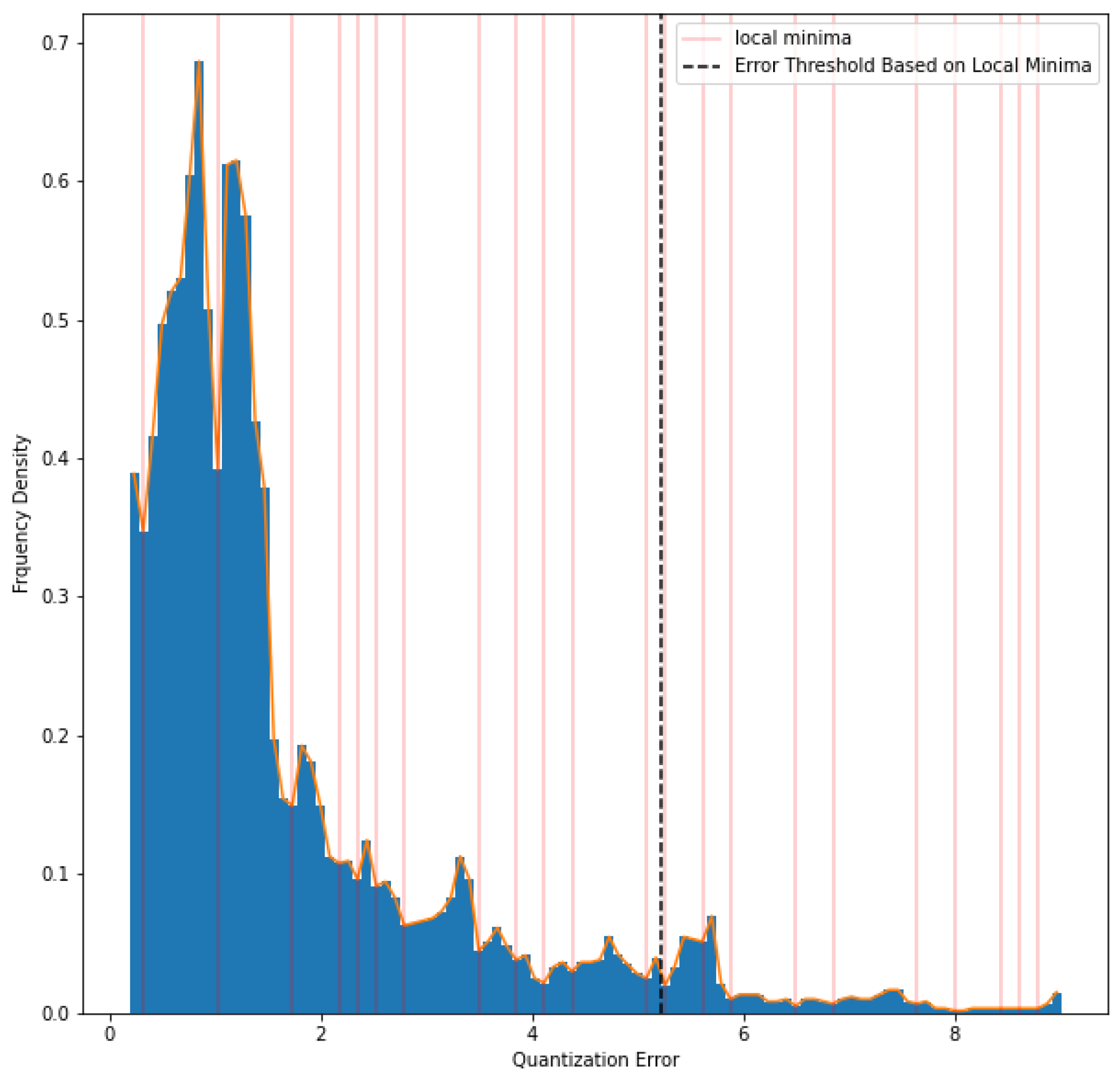
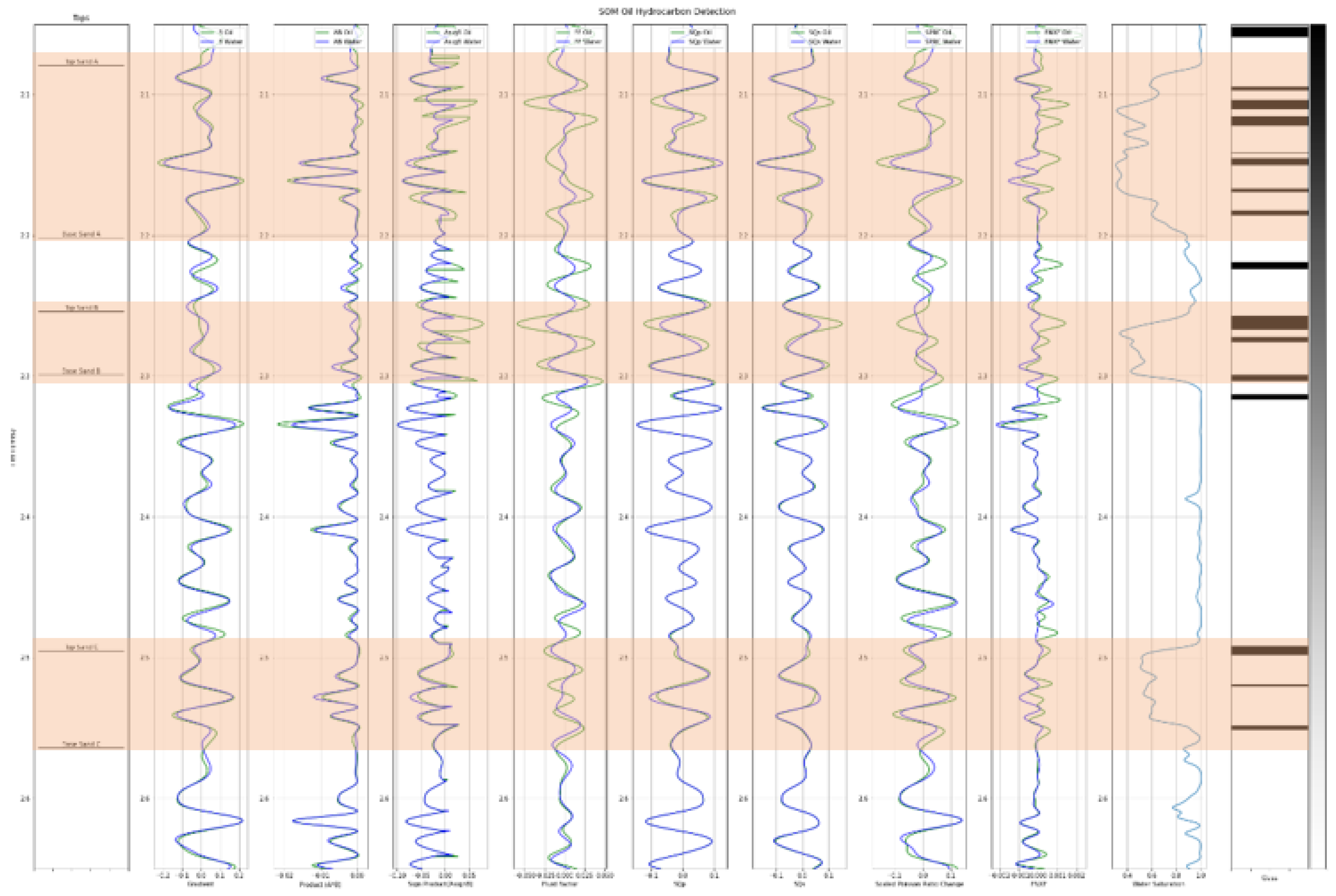
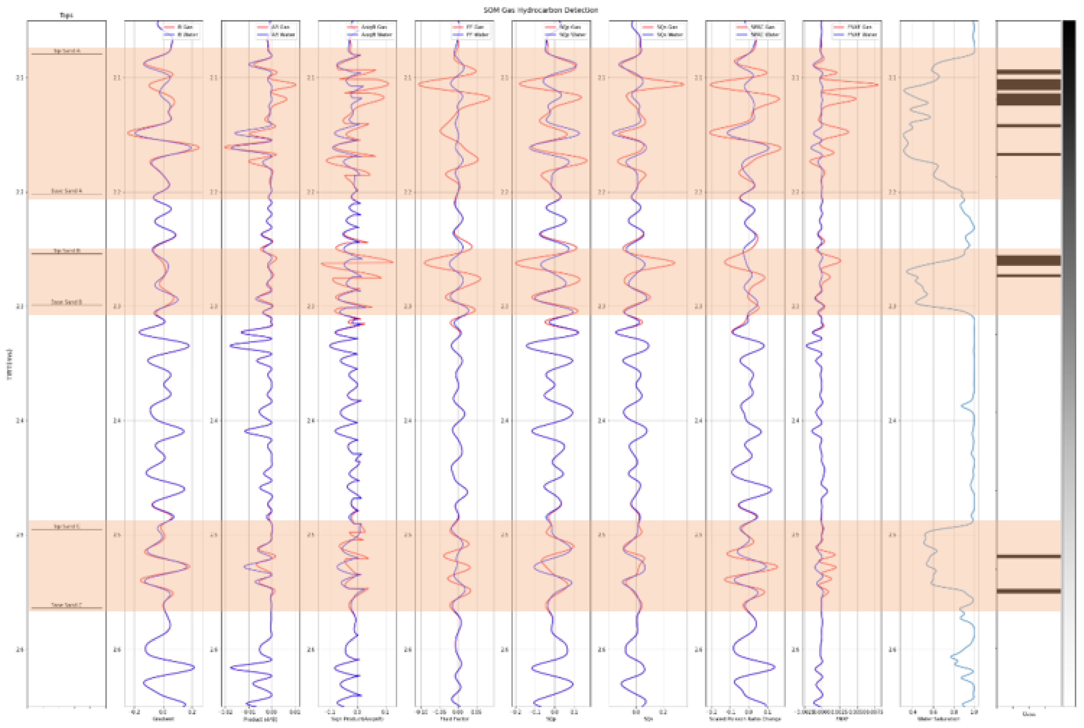
Using this method, the quantization error is used as a metric for anomaly detection. The higher the quantization error is, the farther its data sample from the dataset’s overall distribution. The error threshold needs to be defined to identify the anomaly of the datasets. Error threshold is determined by the local minima detected from the distribution of quantization error (see Figure 8). Figure 9 and Figure 10 below show the result of the hydrocarbon detection using self-organizing maps on the oil and gas conditions, respectively.
From the figures above, the model can delineate hydrocarbons at three reservoir areas in the well log data, especially, in gas condition. The model can also delineate hydrocarbons in the oil condition, although there is a misdelineation. However, overall, the model has done an effective analysis in the well log area with different fluid scenarios. To validate the overall performance of the model, water saturation was used as a validation parameter. For the validation purpose, labelling needs to be conducted where any data sample with less than 0.5 water saturation was be assigned as a hydrocarbon; meanwhile, any data samples with greater than or equal to 0.5 water saturation values were assigned as not a hydrocarbon. The model resulted in an accuracy of 82% in the oil condition and 85% in the gas condition.
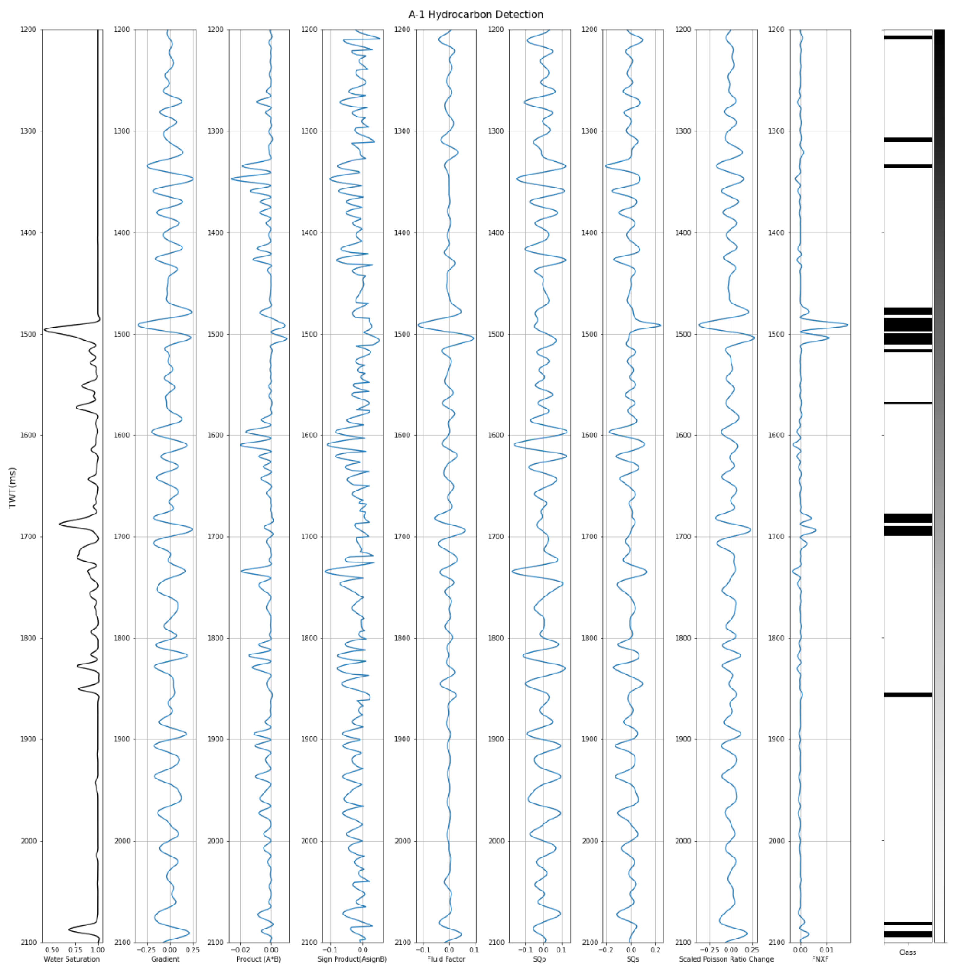
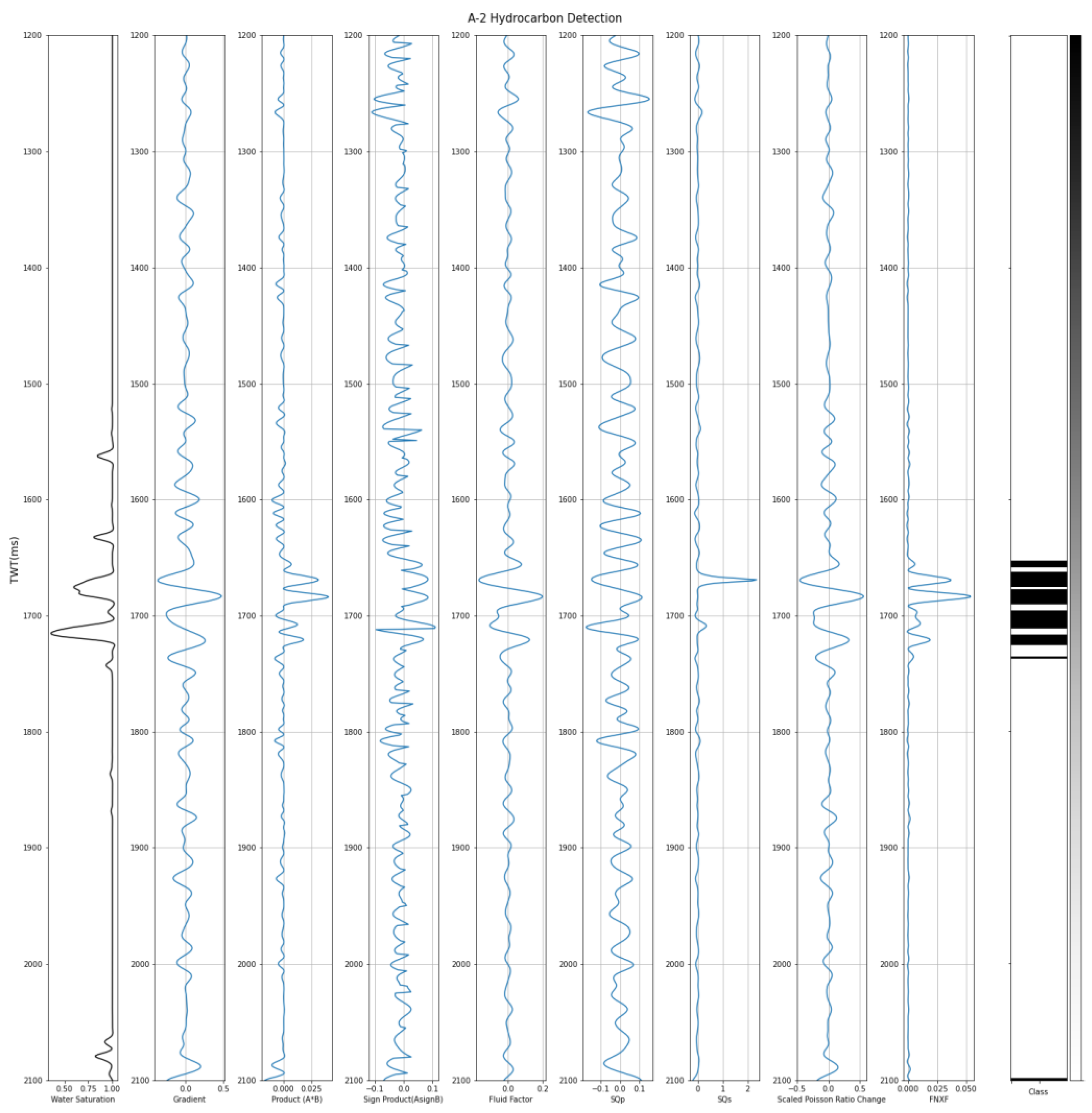
The model was tested in A well area where A-1 and A-2 are used for model testing. To validate the overall performance of the model, water saturation was also used as a validation parameter where any data sample with less than 0.5 water saturation was assigned as a hydrocarbon; meanwhile, any data samples with greater than or equal to 0.5 water saturation values were assigned as not a hydrocarbon. The model resulted in an accuracy of 92% in A-1 and 93% in A-2 (see Figure 11 and Figure 12). Qualitatively, the delineation result matches well with the indication of hydrocarbons from the water saturation log, although there are some misdelineations at the shallow part on well A-1.
5.4. Hydrocarbon Delineation in Seismic Scale
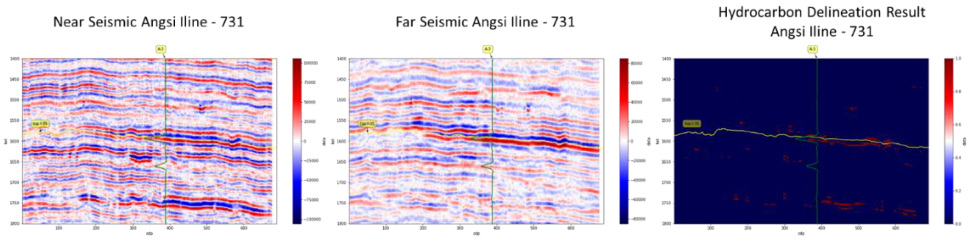
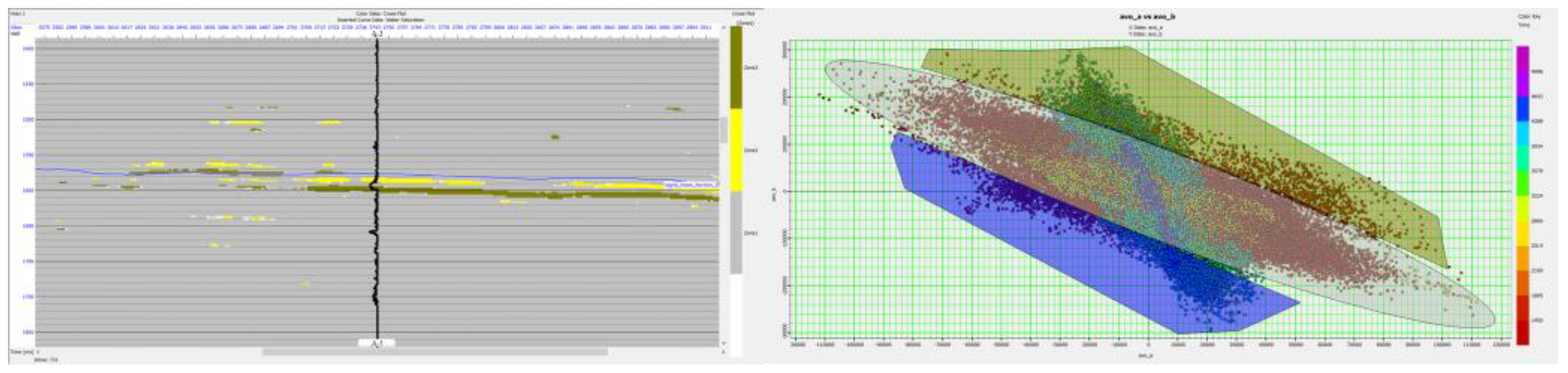
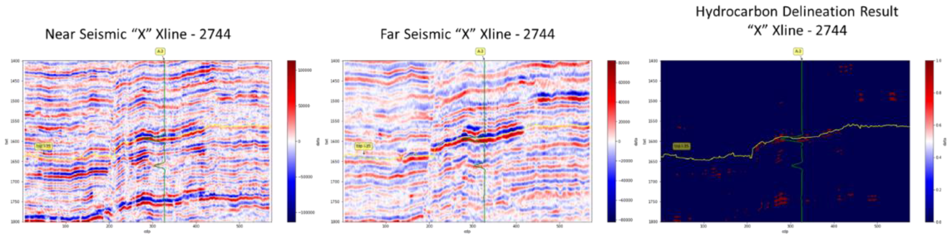
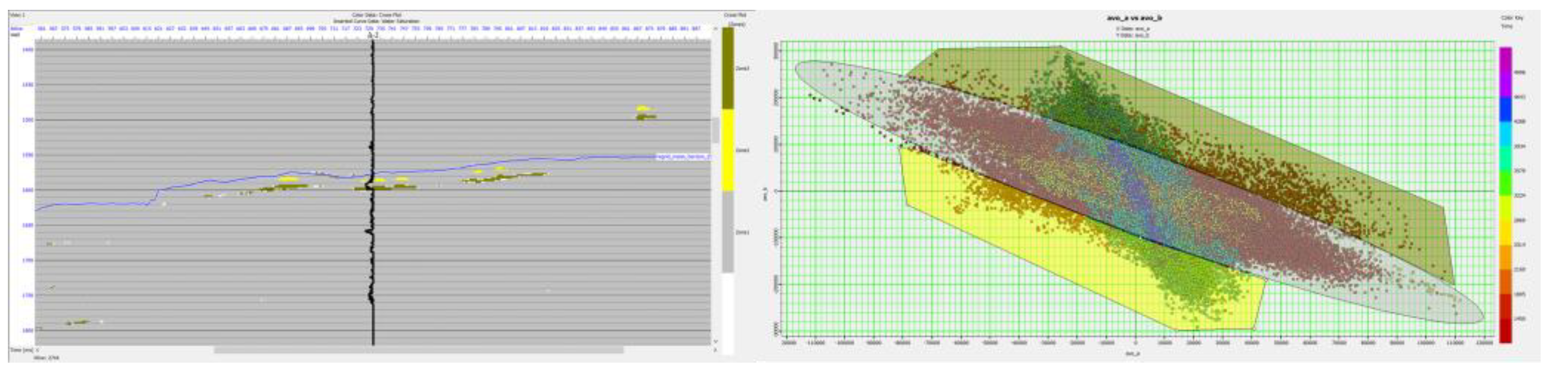
After the model is validated in synthetic seismic, the analysis proceeded to real seismic data. The model was applied in “X” seismic Inline-731 and Xline-2744 where A-3 is located at. The red color in the hydrocarbon delineation result figures (see Figure 13 and Figure 15) indicates a potential hydrocarbon from the SOM. The model was compared with the conventional method where AVO cross-plotting was conducted to delineate potential hydrocarbons (see Figure 13, Figure 14, Figure 15 and Figure 16). For validation purposes, a water saturation log is used for the indication of hydrocarbons at the well area.
From the figures above, the SOM model managed to delineate hydrocarbons in Top I-35 Fm where it was confirmed from the water saturation log, indicating that the formation contains hydrocarbons. Compared with the conventional method by using AVO cross-plotting, the method could also delineate the hydrocarbons at the same area as the SOM does. However, the bias from the interpreter at defining the background of wet sands and shales and the outliers that are typically associated with a hydrocarbon reservoir might affect the delineation result. At the deeper interval around 1750 m, the SOM model indicate a potential hydrocarbon at the northwestern part of A-3. Unfortunately, due to a lack of well log data available, the delineation result could not be verified as to whether there is a hydrocarbon in that area.
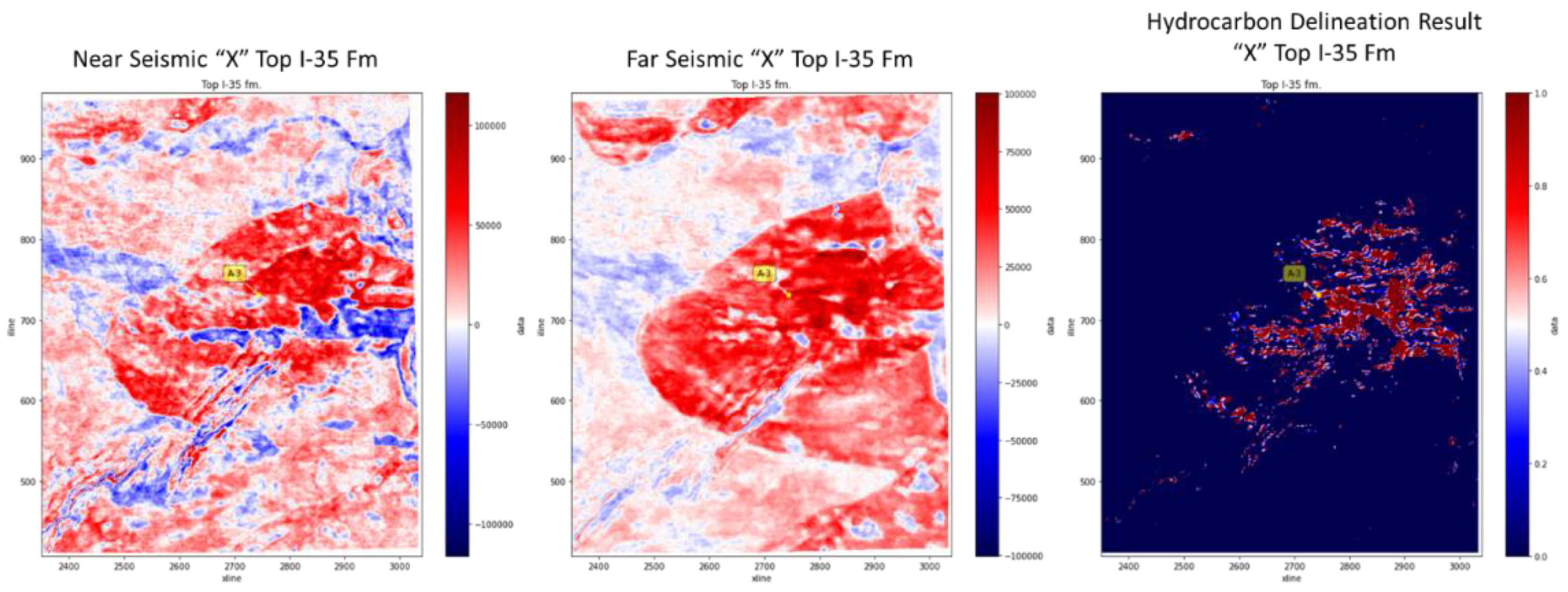
The model delineation result was analyzed in Top I-35 formation (see Figure 17). The hydrocarbon delineation results show in the right figure in Figure 17 where the red color indicates the potential hydrocarbon that was delineated by the SOM model. Unfortunately, it is difficult to conduct a quantitative interpretation in this view. Therefore, the A-3 well location is plotted to confirm the delineation of hydrocarbons since it has been validated from the previous analysis. From the figure above, the model shows that, at the A-3 well log position, hydrocarbon potential could be identified, which was shown as a red color.
6. Conclusions
To detect hydrocarbons, generally, AVO analysis and attributes are used. However, there are still several pitfalls for this method because it requires a great deal of time and experience and subjectiveness as the analysis is completed manually. In this study, an unsupervised learning method was used named self-organizing maps (SOM) to delineate hydrocarbons from given AVO attributes that have been applied to detect hydrocarbons in previous research. From this study, the best selected AVO attributes to detect hydrocarbons using the proposed methods are gradient, product, sign of product, scaled Poisson ratio change, fluid factor, SQp, and SQs. The selected attributes were used as inputs for the anomaly detection model using SOM. In the well log scale analysis, the model worked well to detect hydrocarbons, where the model yielded an average accuracy of 83.5% on fluid replacement modelling well log simulation data. The model was also applied in A-1 and A-2 well log data, where it yielded an average accuracy of 92.5%. After being tested in well log data, the model was applied to real seismic data, where the model can predict the presence of hydrocarbons effectively. The proposed unsupervised learning model can be utilized as an alternative for early detection tools to identify the hydrocarbon presence at the preliminary stage of exploration when there is still no well available.
This research can be elaborated for further development on hydrocarbon delineation by using the semi-supervised machine learning method. A small amount of labeled data to train a machine learning model is a common problem in the application of machine learning in hydrocarbon exploration because it often requires a great deal of experience and is cost ineffective. The current research workflow can be utilized to help labelling more unlabeled data to be used to train the machine learning model combined with the available data. These can potentially increase learning accuracy, creating a more robust model to predict hydrocarbons.
Author Contributions
Conceptualization, L.A.S. and M.H.; methodology, L.A.S. and M.H.; software, L.A.S.; validation, L.A.S. and M.H.; formal analysis, L.A.S. and M.H.; investigation, L.A.S. and M.H.; resources, L.A.S. and M.H.; data curation, L.A.S. and M.H.; writing—original draft preparation, L.A.S.; writing—review and editing, L.A.S., M.H. and I.S.; visualization, L.A.S.; supervision, M.H. and I.S. All authors have read and agreed to the published version of the manuscript.
Funding
This research was funded by UTP fundamental research grant with grant number 015MD0-059.
Institutional Review Board Statement
Not applicable.
Informed Consent Statement
Not applicable.
Acknowledgments
The authors would like to thank PETRONAS Malaysia and Centre for Subsurface Imaging UTP for providing the data for this study. We would like to express our appreciation to Centre for Subsurface Imaging and Geoscience department Universiti Teknologi PETRONAS colleagues for supporting us throughout the project. Huge gratitude to UTP fundamental research grant with cost center 015MD0-059 for granting this research. We acknowledge CGG Company for providing Hampson Russell software licensing, Schlumberger Company for providing Petrel software licensing, and Ikon Science for providing Rokdoc software licensing.
Conflicts of Interest
The authors declare no conflict of interest.
References
- Nanda, N.C. Direct Hydrocarbon Indicators (DHI). In Seismic Data Interpretation and Evaluation for Hydrocarbon Exploration and Production; Springer: Cham, Switzerland, 2016; pp. 103–113. [Google Scholar]
- Rowi, V.; Haris, A.; Riyanto, A. Direct hydrocarbon indicator (DHI) pitfall assessment in prospecting pliocene globigerina biogenic gas play in “x structure”, Madura Strait, East Java Basin. In IOP Conference Series: Earth and Environmental Science; IOP Publishing: Bristol, UK, 2020; Volume 481. [Google Scholar]
- Ross, C.P. Unbiased AVO crossplotting? Lead. Edge 2016, 35, 338–344. [Google Scholar] [CrossRef]
- Lubo-Robles, D.; Ha, T.; Lakshmivarahan, S.; Marfurt, K.J. Supervised seismic facies classification using Probabilistic Neural Networks: Which attributes should the interpreter use? In Proceedings of the SEG International Exposition and Annual Meeting, San Antonio, TX, USA, 15–20 September 2019; pp. 2273–2277. [Google Scholar]
- Roden, R. Seismic interpretation in the age of big data. SEG Tech. Progr. Expand. Abstr. 2016, 35, 4911–4915. [Google Scholar]
- Babikir, I.; Salim, A.; Hermana, M.; Latiff, A.H.A.; Almasgari, A. Multiattribute analysis of a Pleistocene fluvial system using RGB color blending and self-organizing maps. In SEG Technical Program Expanded Abstracts 2020; Society of Exploration Geophysicists: Tulsa, OK, USA, 2020; pp. 1279–1283. [Google Scholar]
- Zhao, T.; Zhang, J.; Li, F.; Marfurt, K.J. Characterizing a turbidite system in Canterbury Basin, New Zealand, using seismic attributes and distance-preserving self-organizing maps. Interpretation 2016, 4, SB79–SB89. [Google Scholar] [CrossRef] [Green Version]
- Borgilchuluun, K.; Cao, D.; Yin, X. Unsupervised learning technique reveals hydrocarbon potential zone on the Penobscot. In Proceedings of the SEG 2018 Workshop: SEG Maximizing Asset Value Through Artificial Intelligence and Machine Learning, Beijing, China, 17–19 September 2018; pp. 53–55. [Google Scholar]
- Zhao, T.; Verma, S.; Qi, J.; Marfurt, K.J. Supervised and unsupervised learning: How machines can assist quantitative seismic interpretation. SEG Tech. Progr. Expand. Abstr. 2015, 34, 1734–1738. [Google Scholar]
- Ciz, R.; Urosevic, M.; Dodds, K. Pore pressure prediction based on seismic attributes response to overpressure. APPEA J. 2005, 45, 449. [Google Scholar] [CrossRef]
- Chadwick, R.A.; Marchant, B.P.; Williams, G.A. CO2 storage monitoring: Leakage detection and measurement in subsurface volumes from 3D seismic data at Sleipner. Energy Procedia 2014, 63, 4224–4239. [Google Scholar] [CrossRef] [Green Version]
- Mahob, P.N.; Castagna, J.P. Avo hodograms and polarization attributes. Lead. Edge 2002, 21, 18. [Google Scholar]
- Hermana, M.; Ghosh, D.P.; Sum, C.W. Discriminating lithology and pore fill in hydrocarbon prediction from seismic elastic inversion using absorption attributes. Lead. Edge 2017, 36, 902–909. [Google Scholar] [CrossRef]
- Hermana, M.; Lubis, L.A.; Ghosh, D.P.; Sum, C.W. New rock physics template for better hydrocarbon prediction. In Proceedings of the Offshore technology conference Asia 2016, OTCA 2016, Houston, TX, USA, 5 May 2016; pp. 2900–2905. [Google Scholar]
- Ridwan, T.K.; Hermana, M.; Lubis, L.A.; Riyadi, Z.A. New avo attributes and their applications for facies and hydrocarbon prediction: A case study from the northern malay basin. Appl. Sci. 2020, 10, 7786. [Google Scholar] [CrossRef]
- Roden, R.; Smith, T.A.; Santogrossi, P.; Sacrey, D.; Jones, G. Seismic interpretation below tuning with multiattribute analysis. Lead. Edge 2017, 36, 330–339. [Google Scholar] [CrossRef]
- Bougher, B.B.; Herrmann, F.J. AVA classification as an unsupervised machine-learning problem. SEG Tech. Progr. Expand. Abstr. 2016, 35, 553–556. [Google Scholar]
- Kohonen, T. The Self-Organizing Map. Proc. IEEE 1990, 78, 1464–1480. [Google Scholar] [CrossRef]
- Kohonen, T. Essentials of the self-organizing map. Neural Netw. 2013, 37, 52–65. [Google Scholar] [CrossRef] [PubMed]
- Ferreira, A.J.; Figueiredo, M.A.T. Efficient feature selection filters for high-dimensional data. Pattern Recognit. Lett. 2012, 33, 1794–1804. [Google Scholar] [CrossRef] [Green Version]
- Katsifarakis, N.; Karatzas, K. A New Feature Selection Methodology for Environmental Modelling Support: The Case of Thessaloniki Air Quality; Springer International Publishing: New York, NY, USA, 2017; Volume 507, ISBN 9783319899343. [Google Scholar]
Figure 1.
AVO classification by identifying the gradient of change in seismic reflection with various angles of incident.
Figure 1.
AVO classification by identifying the gradient of change in seismic reflection with various angles of incident.

Figure 2.
Fluid replacement modelling result on synthetic wells.

Figure 3.
Several AVO attributes extracted from well log data.

Figure 4.
Feature map generated by SOM in oil & gas situation dataset.

Figure 5.
Heatmap correlation of SOM features map.

Figure 6.
Mean–median score analysis on oil & gas condition.

Figure 7.
Selected AVO attributes for anomaly detection.

Figure 8.
Error threshold assignment from quantization error distribution using local minima.

Figure 9.
Hydrocarbon delineation result on oil condition.

Figure 10.
Hydrocarbon delineation result on gas condition.

Figure 11.
Hydrocarbon delineation on A−1.

Figure 12.
Hydrocarbon delineation on A−2.

Figure 13.
Hydrocarbon delineation result on “X” Seismic Inline—731 using SOM.

Figure 14.
Hydrocarbon delineation result on “X” Seismic Inline—731 using AVO cross-plotting.

Figure 15.
Hydrocarbon delineation result on “X” Seismic Xline—2744 using SOM.

Figure 16.
Hydrocarbon delineation result on “X” Seismic Xline—2744 using AVO cross-plotting.

Figure 17.
Hydrocarbon delineation result on Top I−35 Formation.

Publisher’s Note: MDPI stays neutral with regard to jurisdictional claims in published maps and institutional affiliations. |
© 2022 by the authors. Licensee MDPI, Basel, Switzerland. This article is an open access article distributed under the terms and conditions of the Creative Commons Attribution (CC BY) license (https://creativecommons.org/licenses/by/4.0/).
Share and Cite
MDPI and ACS Style
Syahputra, L.A.; Hermana, M.; Satti, I. Pay Zone Determination Using Enhanced Workflow and Neural Network. Appl. Sci. 2022, 12, 2234. https://0-doi-org.brum.beds.ac.uk/10.3390/app12042234
AMA Style
Syahputra LA, Hermana M, Satti I. Pay Zone Determination Using Enhanced Workflow and Neural Network. Applied Sciences. 2022; 12(4):2234. https://0-doi-org.brum.beds.ac.uk/10.3390/app12042234
Chicago/Turabian StyleSyahputra, Loris Alif, Maman Hermana, and Iftikhar Satti. 2022. "Pay Zone Determination Using Enhanced Workflow and Neural Network" Applied Sciences 12, no. 4: 2234. https://0-doi-org.brum.beds.ac.uk/10.3390/app12042234
Note that from the first issue of 2016, this journal uses article numbers instead of page numbers. See further details here.