Balance Control of a Quadruped Robot Based on Foot Fall Adjustment

Abstract

To balance the diagonal gait of a quadruped robot, a dynamic balance control method is presented to improve the stability of the quadruped robot by adjusting its foot position. We set up a trunk-based coordinate system and a hip-based local coordinate system for the quadruped robot, established the kinematics equation of the robot, and designed a reasonable initial diagonal gait through the spring inverted pendulum model. The current trunk posture of the quadruped robot is obtained by collecting the data of its pitch and roll angle, and the foot position is predicted according to the current posture and initial gait of the quadruped robot. To reduce the impact of one leg landing on the ground and increase the stability of the quadruped robot, we adjust the landing point of the robot according to the landing time difference between the diagonal legs. The proposed method can adjust the body in such scenarios as planar walking and lateral impact resistance. It can reduce the disturbance during the robot motion and make the robot move smoothly. The validity of this method is verified by simulation experiments.

1. Introduction

Mobile robots can be divided into three types: legged-foot, caterpillar, and wheeled. Compared with caterpillar and wheeled robots, legged-foot robots have discrete landing locations and can choose the best landing locations for support. Therefore, legged-foot robots have more advantages in terrain adaptability, motion flexibility, and load capacity. They have broader application prospects in the fields of material transportation, military investigation, field exploration, rescue, and disaster relief.

The first real quadruped robot research began in the 1960s. After more than half a century of development, various styles of quadruped robots emerged. At present, one of the most representative quadruped robots is the BigDog series developed by Boston Dynamics [1,2]. They have good topographic adaptability, load capacity, impact resistance. They can walk and trot under more complex terrain such as gravel, grassland, snow, etc. Starting in 2015, Boston Dynamics introduced the Spot series of quadruped robots, which are small, powerful, and flexible [3,4]. ANYmal, a quadruped robot developed by the Swiss Federal Institute of Technology Zurich (ETH Zurich), has improved the series elastic driver to achieve more flexible and precise moment control. It has a laser sensor and a camera installed on its body to sense the terrain of the environment for map building and self-positioning [5]. The Cheetah series quadruped robots, developed by the Massachusetts Institute of Technology (MIT), mimic the body structure of a cheetah. It can run at high speed, up to 6 m/s. In 2019, MIT launched Mini Cheetah, the first quadruped robot that can flip backward. It can move horizontally, jump, climb from a fall, and flip backward without visual aids. It has epochal significance in robotics.

Balance control of quadruped robots is one of the research hotspots in the field of motion control of quadruped robots. Currently, there are many ways to control robot body balance. The classical control methods include Zero Moment Point (ZMP) [6,7,8], Virtual Model Control (VMC) [9,10,11], Central Pattern Generator (CPG) [12,13], and Spring Loaded Inverted Pendulum (SLIP) [14,15,16].

ZMP is mostly used in static gait, which requires calculating the ZMP position of the quadruped robot so that the ZMP point is always inside the polygon formed by the support point at the foot of the robot to ensure that the robot has a static balance state [17]. In [7], an LIP model of the robot was combined with the ZMP calculation to derive joint space control action based on a PD controller. The anti-interference ability of the robot is enhanced and the stability is improved. In [8], a gait planning method and a posture adjustment strategy were designed based on the ZMP stability criterion, which can improve the stability and obstacle crossing ability of the quadruped robot effectively. However, ZMP is mostly suitable for the balance control of static gait and cannot meet the needs of the fast motion of the robot. The core idea of VMC is to drive the robot to produce the desired action by generating corresponding virtual force from virtual components. In [10], an improved VMC control method was proposed, which can realize stable walking of quadruped robot with dynamic gait and have a low computational cost. In [11], a fractional-order VMC (FOVMC) for quadruped robot trotting motion was proposed. The fractional-order virtual damper was integrated with the classical VMC, the robustness and accuracy of VMC were improved effectively. However, the main problem of VMC is still high computing cost and response lag. In [14], a new template model called Spring Loaded Inverted Pendulum with Swing Legs (SLIP-SL) was proposed, which was improved on the popular SLIP model by adding passive swing leg dynamics. Based on the SLIP model, quadruped robots such as Spot, SpotMini, etc. show excellent motion performance.

In previous studies, the criteria to judge the stability of quadruped robot walking are mostly applicable to static gait. For dynamic gait, there is no specific method to measure stability. In this paper, the flight rate is used as an index to reflect the stability of the robot’s dynamic gait. By adjusting the robot’s landing point, the impact of the ground on one leg landing first is reduced. This method improves the stability of quadruped robots.

In this paper, a dynamic balance control method for the quadruped robot walking in diagonal gait was proposed. Firstly, the initial diagonal gait of the quadruped robot was planned through modeling and kinematics. The foot position was predicted according to the current body posture. Then, the landing point of the quadruped robot was adjusted according to the landing time difference between the diagonal legs to achieve the stable motion of the quadruped robot. Experiments show that the method can significantly improve the stability of the quadruped robot under diagonal gait, reduce the adjustment time and improve the anti-interference ability.

2. Dynamics of Quadruped Robots

2.1. Simulation Model Analysis

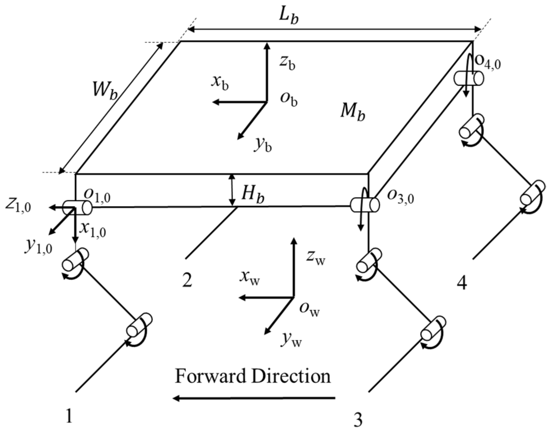
We built a simplified model of a quadruped robot modeled after Billy the robot Dog, which is shown in Figure 1. The model is composed of the trunk, joints, large and small legs, and other components. Based on the forward direction, the lef-front leg, right-front leg, left-rear leg, and right-rear leg are numbered as 1, 2, 3, and 4, respectively. The base coordinate system $\left\{O_w\right\}$ is on the ground, the trunk coordinate system $\left\{O_b\right\}$ is established at the geometric center of the trunk, and the leg base coordinate system $\left\{O_{i,0}\right\}$ is established at the joint between the hip joint and the trunk, where $i=1, 2, 3, 4$.

The model uses the D-H method to determine the pose relationship between various components of the robot. Its single leg model is shown in Figure 2. Each leg has three degrees of freedom, including hip, knee, and ankle. The coordinate system of the body’s leg $i$ is established according to the single-leg model. The leg base coordinate system $\left\{O_{i,1}\right\}$ is established at the hip joint. The coordinate system $\left\{O_{i,2}\right\}$, $\left\{O_{i,3}\right\}$ is established at the knee joint and ankle joint, respectively. The coordinate system $\left\{O_{i,4}\right\}$ is established at the end of the foot. The z-axis of the three coordinate systems is the rotation axis of the corresponding joint, ${\theta }_{i,k}$ represents the rotation angle from $x_{i,k-1}$ to $x_{i,k}$ around $z_{i,k}$. The x-axis of the three coordinate systems is on the connecting rod of each joint, and the direction is shown in Figure 2. The y-axis of the three coordinate systems is determined by the right-hand rule. The length of each connecting rod of the leg is represented by $L_1$, $L_2$, and $L_3$, and its mass corresponds to $m_1$, $m_2$, and $m_3$ respectively.

According to the link length and joint angle, the position of the robot’s foot point in the body coordinate system is calculated, so as to analyze the motion trajectory of the quadruped robot. The motion of the quadruped robot is analyzed according to the forward kinematics equation, and the pose relationship from the foot end coordinate system $\left\{O_{i,4}\right\}$ to the leg base coordinate system $\left\{O_{i,0}\right\}$ is calculated. The homogeneous transformation matrix is:

$${}_4{}^{0}T{}_i=[\begin{array}{cccc}{c}_{i,1}{c}_{i,23}& -c_{i,1}{s}_{i,23}& -s_{i,1}& c_{i,1}{L}_1+c_{i,1}{c}_{i,2}{L}_2+c_{i,1}{c}_{i,23}{L}_3\\ s_{i,1}{c}_{i,23}& -s_{i,1}{s}_{i,23}& c_{i,1}& s_{i,1}{L}_1+s_{i,1}{c}_{i,2}{L}_2+s_{i,1}{c}_{i,23}{L}_3\\ -s_{i,23}& -c_{i,23}& 0& -s_{i,2}{L}_2-s_{i,23}{L}_3\\ 0& 0& 0& 1\end{array}$$

(1)

where: $c_{i,1}=\cos {\theta }_{i,1},c_{i,23}=\cos ({\theta }_{i,2}+{\theta }_{i,3}),s_{i,1}=\sin {\theta }_{i,1},s_{i,23}=\sin \left({\theta }_{i,2}+{\theta }_{i,3}\right)$

According to Formula (1), the positional relationship between the end coordinates of each foot and the leg base coordinate system can be obtained:

$$P_i=\left[\begin{array}{c}{x}_i\\ y_i\\ z_i\\ 1\end{array}\right]=\left[\begin{array}{c}{c}_{i,1}{L}_1+c_{i,1}{c}_{i,2}{L}_2+c_{i,1}{c}_{i,23}{L}_3\\ s_{i,1}{L}_1+s_{i,1}{c}_{i,2}{L}_2+s_{i,1}{c}_{i,23}{L}_3\\ -s_{i,2}{L}_2-s_{i,23}{L}_3\\ 1\end{array}\right]$$

(2)

.

If the foot position of the robot is given, the rotation angle of each joint of the robot can be solved through the inverse kinematics equation:

$$\left\{\begin{array}{c}{\theta }_{i,1}={\tan }^{-1}(\frac{y_i}{x_i})\\ {\theta }_{i,2}={\sin }^{-1}[\frac{-L_3{s}_{i,3}}{\sqrt{{(L_1-x_i{c}_{i,1}-y_i{s}_{i,1})}^2+z_i{}^2}}]-{\tan }^{-1}(\frac{z_i}{x_i{c}_{i,1}+y_i{s}_{i,1}-L_1})\\ {\theta }_{i,3}={\cos }^{-1}[\frac{{(x_i{c}_{i,1}+y_i{s}_{i,1}-L_1)}^2+z_i{}^2-L_2{}^2-L_3{}^2}{2L_2{L}_3}]\end{array}\right.$$

(3)

2.2. Gait Planning

To keep the quadruped robot balanced during a trot, the center of gravity should be placed on the diagonal of the support phase. Due to errors in the trot movement, the center of gravity cannot be kept on the diagonal at all times. To make the robot move steadily, it is necessary to reasonably plan the foot coordinate trajectory when the swinging phase is transformed into the supporting phase. The two legs on the diagonal are called diagonal legs, and the quadruped robot has two groups of diagonal legs. To simplify the control algorithm of quadruped movement, we introduce the concept of a virtual leg. In trot gait, the diagonal legs have the same movement form and the hip joint exerts similar force on the trunk, so the two legs on the diagonal can be equivalent to a virtual leg [18,19]. After equivalence, the two virtual legs are also on the diagonal and can be further equivalent to a virtual leg, as shown in Figure 3:

To balance the trunk posture, PD (proportional-differential) control of trunk posture is added to the foot-end planning of the supporting phase. Based on the kinematics model of the robot, the trot trajectory of the quadruped robot is proposed. During the motion of the robot, each foot periodically sways relative to the trunk of the quadruped robot. The quadruped robot can move at a steady and uniform speed and can pass through the slightly undulating ground. The characteristics of the robot’s foot trajectory during the motion are analyzed:

(1)

The speed of the swing leg decreases to zero when it falls on the ground.

(2)

Keep the supporting legs moving at a constant speed during the retraction process.

(3)

There should be no abrupt change in the speed and acceleration of the swing leg and supporting leg during movement.

In order to ensure the continuity of the body in the process of movement, the method of combining a cubic spline and a straight line is used to plan the foot trajectory. It is assumed that the step length of the foot target trajectory is S, the step height is H, the initial position of the foot end is (−20, 0, 0), the unit is mm, the velocity and acceleration at the beginning and end are 0, and the movement period is T. The fitted curve of foot end trajectory of the quadruped robot is realized.

The trajectory of the robot’s supporting leg is defined as:

$$\begin{array}{c}x\left(t\right)=S\times \left(3-\frac{4t}{T}\right) \left(\frac{T}{2}<t\le T\right)\\ z\left(t\right)=0 (\frac{T}{2}<t\le T)\end{array}$$

(4)

The trajectory of robot’s swinging leg is defined as:

$$\begin{array}{c}x\left(t\right)=S\times \left(-64\times \frac{t^3}{T^3}+48\times \frac{t^2}{T^2}-4\times \frac{t}{T}-1\right) (0<t\le \frac{T}{2})\\ z\left(t\right)=\left\{\begin{array}{c}H\times \left(-128\times \frac{t^3}{T^3}+48\times \frac{t^2}{T^2}\right) 0<t\le \frac{4}{T}\hfill \\ H\times \left(128\times {\left(\frac{t}{T}-\frac{T}{4}\right)}^3-48\times {\left(\frac{t}{T}-\frac{T}{4}\right)}^2+1\right) \frac{T}{4}<t\le \frac{T}{2}\end{array}\right.\end{array}$$

(5)

where, $t$ represents the sampling time of gait trajectory.

3. Dynamic Balance Control Method

The diagonal gait can be equivalent to a virtual leg. Ideally, the diagonal legs soar and land at the same time. However, in fact, during the trot process of the quadruped robot, one leg always lands first in the falling process. As shown in Figure 4, the leg that lands first will be impacted by the ground, causing body shake and affecting the stability of the robot’s movement.

According to the above problems, a method is proposed to use flight rate as a stability index to describe the landing condition of the diagonal leg, and the value range of flight rate $\lambda$ is 0–1.

$$\lambda =\frac{t_s}{t}$$

(6)

where, $t_s$ is the flighting time and $t$ is half cycle.

In order to keep the quadruped robot moving stably during diagonal walking, the diagonal legs need to land at the same time to improve the flight rate. The landing attitude of the swing leg is controlled through attitude feedback, as shown in Figure 5:

In Figure 5, 1 and 4 represent the left-front leg and right-rear leg of the quadruped robot. During the walking process, the trunk roll angle is ${\theta }_{roll}$ and the pitch angle is ${\theta }_{pitch}$. The robot length is $L_b=2L^{\prime }$ and width is $W_b=2W^{\prime }$, $H$ is the height of the robot centroid, $h^{\prime }$ represents the height of the 1 leg and $h^{″}$ represents the height of the 4 leg. $l^{\prime }$ and $l^{″}$ represent the front-back moving distance of 1 and 4 legs, respectively. It can be concluded that:

$$\begin{array}{c}\left\{\begin{array}{c}{l}^{\prime }=x_{01}-h^{\prime }\tan \left({\theta }_{pitch}\right)\hfill \\ h^{\prime }=z_{01}+W^{\prime }\sin \left({\theta }_{roll}\right)+L^{\prime }\sin \left({\theta }_{pitch}\right)\hfill \end{array}\right.\hfill \\ \left\{\begin{array}{c}{l}^{″}=x_{04}-h^{″}\tan \left({\theta }_{pitch}\right)\hfill \\ h^{″}=z_{04}-W^{\prime }\sin \left({\theta }_{roll}\right)-L^{\prime }\sin \left({\theta }_{pitch}\right)\hfill \end{array}\right.\end{array}$$

(7)

The quadruped robot can predict the best landing point through formulas (7), and the prediction results are shown in

Table 1. The landing points.

	${\mathit{x}}_{\mathit{i}}$	${\mathit{y}}_{\mathit{i}}$	${\mathit{z}}_{\mathit{i}}$
$Left fore$	$x_{01}-\delta z_{01}\tan ({\theta }_{pitch})$	$y_{01}$	$z_{01}+\delta \left(W^{\prime }\sin ({\theta }_{roll}\right)+L^{\prime }\sin ({\theta }_{pitch}))$
$Right fore$	$x_{02}-\gamma z_{02}\tan ({\theta }_{pitch})$	$y_{02}$	$z_{02}+\gamma \left(W^{\prime }\sin ({\theta }_{roll}\right)+L^{\prime }\sin ({\theta }_{pitch}))$
$Left hind$	$x_{03}-\gamma z_{03}\tan ({\theta }_{pitch})$	$y_{03}$	$z_{03}-\gamma \left(W^{\prime }\sin ({\theta }_{roll}\right)+L^{\prime }\sin ({\theta }_{pitch}))$
$Right hind$	$x_{04}-\delta z_{04}\tan ({\theta }_{pitch})$	$y_{04}$	$z_{04}-\delta \left(W^{\prime }\sin ({\theta }_{roll}\right)+L^{\prime }\sin ({\theta }_{pitch}))$

below:

$x_i,y_i,z_i$ represent the $x,y,z$ coordinate axes at the end of the leg $i$, $x_{0i},y_{0i},z_{0i}$ represent the starting $x,y,z$ coordinate axes at the end of the leg $i$. $i$ take $1, 2, 3, 4$ to represent the left-front leg, the right-front leg, the left-rear leg, and the right-rear leg, respectively. $\delta$ and $\gamma$ are coefficients, as follows:

$$\begin{array}{c}\delta =\left\{\begin{array}{c}0 i=2.3\\ 1 i=1.4\end{array}\right.\\ \gamma =\left\{\begin{array}{c}0 i=1.4\\ 1 i=2.3\end{array}\right.\end{array}$$

(8)

The stable condition of the body in diagonal gait is that the diagonal legs are raised and landed at the same time, that is, the flight rate $\lambda$ is equal to 1 as far as possible. In other words, the projection of the body’s gravity center on the support plane should be close to the diagonal line. Therefore, the robot’s gravity center is self-balanced by adjusting the time difference of the robot’s diagonal legs.

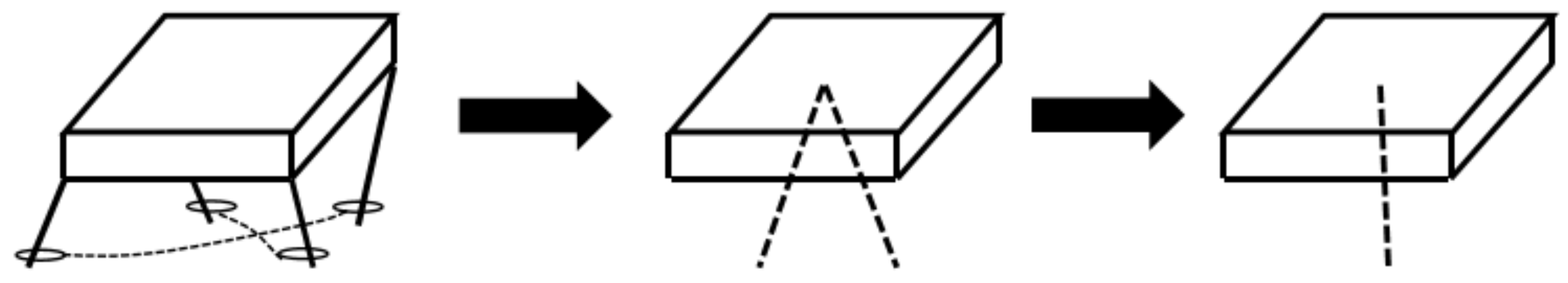
The four cases of gravity center distribution are shown in Figure 6:

The diagonal line of void points represents the moment when the robot’s diagonal legs fall from air to ground, and the diagonal line of solid points represents the moment when the robot’s diagonal legs rise from support ground to air. $O$ is the intersection of two diagonal lines, $a$ is the intersection of the centerline and the 1–4 leg diagonal legs, $b$ is the intersection of the centerline and the 2–3 leg diagonal, $O_1$ is the center of gravity, $l_1$ is the distance from the gravity center of robot to the 1–4 leg diagonal, $l_2$ is the distance from the gravity center of robot to the 2–3 leg diagonal, $d_1$ is the distance from the gravity center of robot to $a$, $d_2$ is the distance from the gravity center of robot to $b$, $\phi$ represents the angle between two diagonals, ${\phi }_1$ represents the angle between the centerline and the 1–4 leg diagonal. ${\phi }_2$ represents the angle between the centerline and 2–3 leg diagonal. According to the movement characteristics of the quadruped robot’s diagonal gait, there is no displacement in the y-axis during movement, so the movement of the robot’s gravity center is always on the centerline. If the center of gravity is not on the line of the diagonal leg that is about to fall, one of the swinging legs touches the ground first, and the impact from the ground causes instability of the trunk [20].

Set the touchdown time of legs 1, 2, 3, and 4 as $t_1$, $t_2$, $t_3$, and $t_4$ respectively. When legs 1 and 4 are in a swing state, the time difference between them touching the ground is expressed as:

$$\mathsf{\Delta }{t}_{14}=t_1-t_4$$

(9)

When legs 2 and 3 are in a swing state, the time difference between them touching the ground is expressed as:

$$\mathsf{\Delta }{t}_{23}=t_2-t_3$$

(10)

The values of $l_1$ and $l_2$ are estimated according to the landing time difference. The greater $l_1$ is, the greater the torque of gravity on 1–4 leg diagonal, and the greater the absolute value of the time difference $\mathsf{\Delta }{t}_{23}$ between leg 2 and 3. Similarly, the greater $l_2$ is, the larger $\mathsf{\Delta }{t}_{14}$ is. $l_1$ and $l_2$ can be estimated as follows:

$$\begin{array}{c}{l}_1=k_1{t}_{23}=k_1\left(t_2-t_3\right)\\ l_2=k_2{t}_{14}=k_2\left(t_1-t_4\right) \end{array}$$

(11)

where, $k_1$ and $k_2$ are proportional coefficients with values greater than 0.

Analyze the four conditions of the gravity center in Figure 6 respectively:

(a)

The projection point of the gravity center is in front of the 2–3 leg diagonal.

When the robot’s gravity center is projected in front of the 2–3 leg diagonal, the distance $d_2$ between the gravity center on centerline and the 2–3 leg diagonal is as follows:

$$d_2=\frac{k_2\left(t_2-t_3\right)}{\sin {\phi }_2}$$

(12)

Since the center of gravity is in front of the 2–3 leg diagonal, leg 2 falls first and leg 3 falls later, $t_2<t_3$. It can be known from the above formula that $t_2-t_3<0,$ $d_2<0$.

(b)

The projection point of the gravity center is behind the 2–3 leg diagonal.

When the robot’s gravity center is projected behind the 2–3 leg diagonal, the distance $d_2$ between the gravity center on the centerline and the 2–3 leg diagonal can be calculated by Formula (12).

Since the center of gravity is behind the 2–3 leg diagonal, leg 3 falls first and leg 2 falls later, $t_2>t_3$. It can be known from Formula (12) that $t_2-t_3>0,$ $d_2>0$.

(c)

The projection point of the gravity center is in front of the 1–4 leg diagonal

When the robot’s gravity center is projected in front of the 1–4 leg diagonal, the distance $d_1$ between the gravity center on the centerline and the 1–4 leg diagonal is as follows:

$$d_1=\frac{k_1\left(t_1-t_4\right)}{\sin {\phi }_1}$$

(13)

Since the center of gravity is in front of the 1–4 leg diagonal, leg 1 falls first and leg 4 falls later, $t_1<t_4$. It can be known from Formula (13) that $t_1-t_4<0,$ $d_1<0$.

(d)

The projection point of the gravity center is behind the 1–4 leg diagonal.

When the robot’s gravity center is projected behind the 1–4 leg diagonal, the distance $d_1$ between the gravity center on the centerline and the 1–4 leg diagonal can be calculated by Formula (13).

Since the center of gravity is behind the 1–4 leg diagonal, leg 4 falls first and leg 1 falls later, $t_1>t_4$. It can be known from Formula (13) that $t_1-t_4>0,$ $d_1>0$.

We analyze the different projection positions of the gravity center and estimate the distance between the projection point of the gravity center and the diagonal of the landing leg on the centerline by foot landing time difference.

The gravity center position is estimated according to the landing time difference of diagonal legs during the quadruped robot movement. After obtaining the estimated position of the gravity center position, the foot position of the quadruped robot is adjusted during the movement to make the landing difference gradually decrease to be stable. The position adjustment of the robot’s gravity center is realized by the movement of the supporting phase. After one cycle of movement, the robot estimates the gravity center position according to the time difference of falling foot and adjusts the foot position. In the next cycle, the center of gravity is re-estimated and adjusted, so that the center of gravity gradually moves to the line of the landing diagonal leg, as shown in Figure 7:

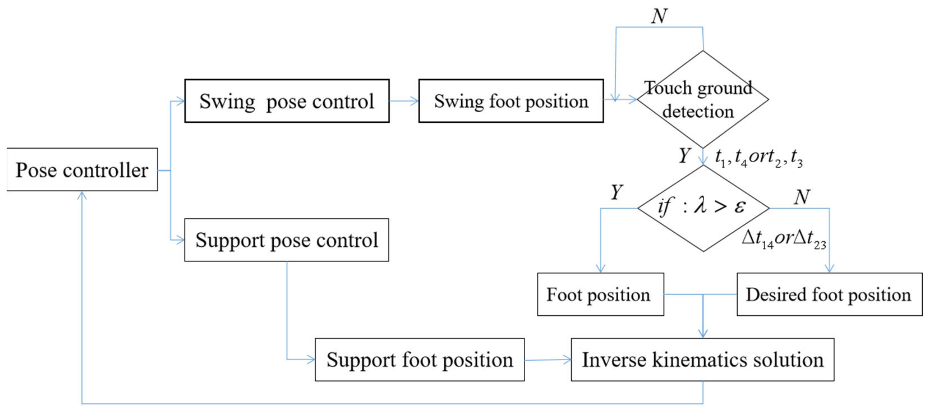
Due to the uncertain position of the gravity center in the early movement stage, one of the robot legs lands first, which leads to a reaction force from the ground. To reduce the reaction force on the leg, the attitude feedback strategy mentioned above is used to make the gravity center adjust smoothly. Gait adjustment strategy flowchart is designed as shown in Figure 8:

(1)

In a cycle, the time difference $\mathsf{\Delta }{t}_{14}$ can be obtained when legs 1 and 4 are in the swinging phase, and the time difference $\mathsf{\Delta }{t}_{23}$ can be obtained when legs 2 and 3 are in the swinging phase.

(2)

According to the landing time difference, the distance $d_1$ or $d_2$ between the projection point of the gravity center and the diagonal of the landing leg on the centerline is solved. Assuming that the initial position before adjustment is $P_i=\left(x_i,y_0\right)$, the desired foot position is:

$$\begin{array}{c}{x}_{ie}=\left\{\begin{array}{c}{x}_0+d_1 i=2.3\\ x_0+d_2 i=1.4\end{array}\right.\\ z_{ie}=z_0+z_{0i}^{\prime }\end{array}$$

(14)

where, $P_i^{\prime }=\left(x_i^{\prime },y_0\right)$ is the desired foot position.

(3)

After the expected foot position of the quadruped robot is calculated, the landing attitude of the swinging leg is adjusted according to the data feedback of the attitude to reduce the force on the leg. Set the expected coordinate value $Q_i^{\prime }=\left(x_{ie},y_0,z_{ie}\right)$, and the expected value of each coordinate axis is:

$$\begin{array}{c}{x}_{ie}=\left\{\begin{array}{c}{x}_0+d_1+x_{0i}^{\prime } i=2,3\\ x_0+d_2+x_{0i}^{\prime } i=1,4\end{array}\right.\\ z_{ie}=z_0+z_{0i}^{\prime } \end{array}$$

(15)

where, $x_{0i}^{\prime }$ and $z_{0i}^{\prime }$ represent the changes in x- and z-axis adjustment, respectively.

(4)

Repeat steps (1) to (3) until the flight rate $\lambda$ is greater than $\epsilon$. $\epsilon$ is an adjustable threshold. When the flight rate is greater than $\epsilon$, it means that the landing time difference of diagonal legs is very small in the movement, and the posture of the body can meet the requirements.

4. Simulation Experiments

In this section, the proposed method will be evaluated in a simulation environment. We introduce the simulation model of the quadruped robot and then test it in two simulation scenarios.

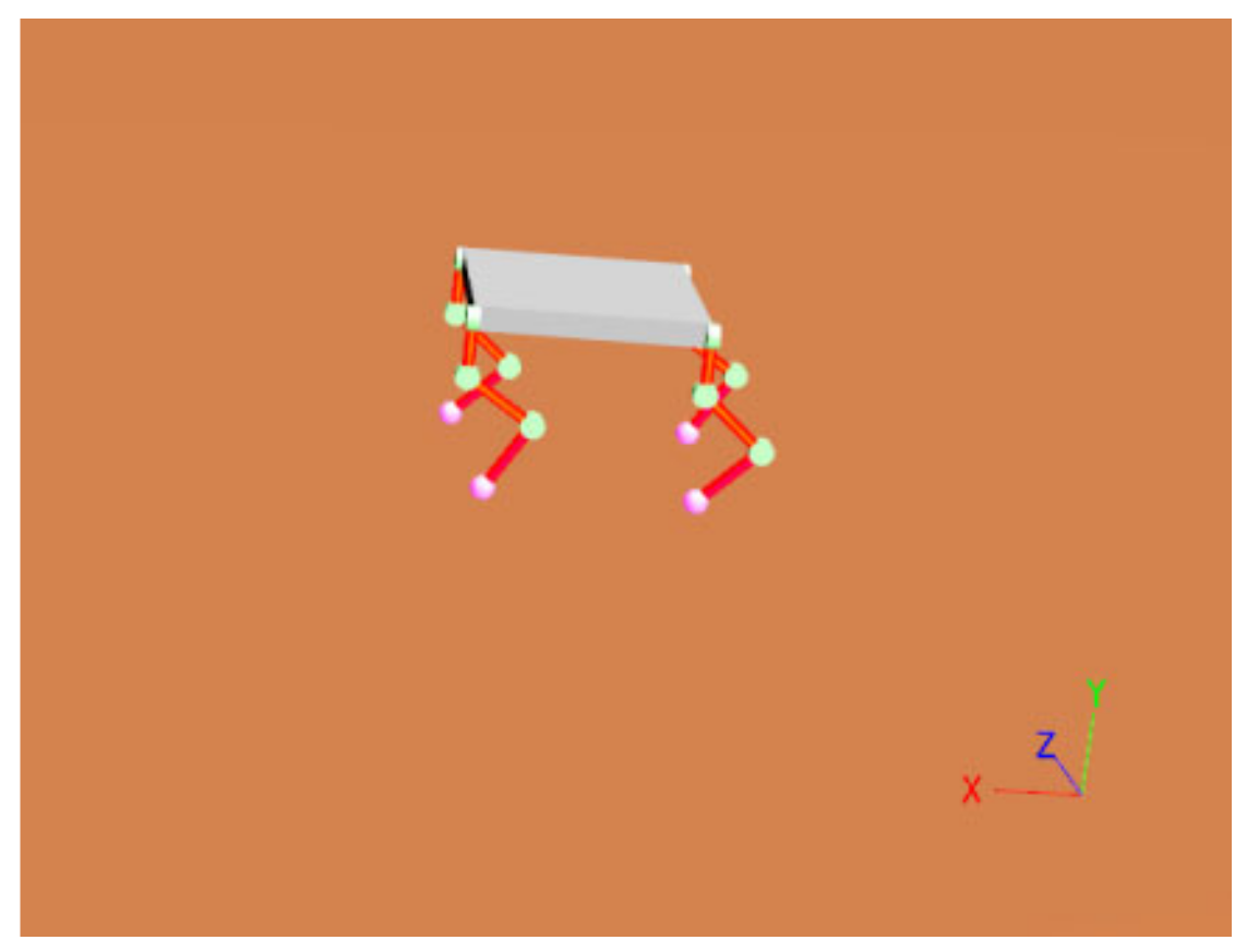
We conduct simulation verification on Webots simulation software, the physics simulation of the robot is shown in Figure 9. The model is composed of the fuselage, joints, and connecting rods, each leg has three degrees of freedom, including hip joint, knee joint, and ankle joint. The test scenarios are flat ground walking and lateral impact simulation. According to the curves of robot roll angle and pitch angle obtained by simulation, the validity of the method is verified. In the simulation environment, gravity acceleration, the friction coefficient between contact surfaces, and other parameters are the default values of the simulation system.

The length and mass parameters of the quadruped robot in the simulation are shown in

Table 2. Parameters in the simulation.

	Parameters	Value
Mass	$M_b$(Trunk)	3 kg
	$m_1$	0.06 kg
	$m_2$	0.12 kg
	$m_3$	0.12 kg
Length	$L_b$(Trunk length)	183 mm
	$W_b$(Trunk width)	162 mm
	$H_b$(Trunk height)	20 mm
	$l_1$	47.5 mm
	$l_2$	65 mm
	$l_3$	65 mm

.

4.1. Flat Ground Walking Simulation

To verify the effectiveness of the proposed method when a quadruped robot walks on flat ground, a set of comparative simulation experiments are set up: stability tests with foot adjustment strategy and stability tests without foot adjustment strategy, and stability analysis is carried out through changing in roll angle and pitch angle.

In this simulation, Formulas (4) and (5) are used to plan the foot trajectory of quadruped robot, the step length S and step height H are set as 40 mm, 40 mm. $k_1$ and $k_2$ in formula (11) are set as 20, 20. $\epsilon$ is set as 0.95. The robot’s change process with the adjustment strategy is shown in Figure 10:

The varied curves of robot roll angle and pitch angle are in Figure 11:

As shown in Figure 10 and Figure 11, at the beginning of the simulation, the robot is in the air 50 mm away from the ground, and each joint of the robot is in position 0. The robot needs a transition process from the standing state to the diagonal walking state. Therefore, the robot’s roll angle and pitch angle change greatly in the beginning period. After a period of time, the roll angle and pitch angle tend to be stable. Combined with Figure 10 and Figure 11, it can be seen that it takes about 4 s for the robot to fall from the standing state to the stable walking state without adding adjustment strategy. However, with the addition of adjustment strategy, it only takes about 1 s for the robot to fall from the standing state to the stable walking state. In the case of no adjustment strategy, the maximum roll angle change is 3.6 degrees, and the maximum pitch angle change is 6.4 degrees, after the stable walking, the robot roll angle fluctuates between $-0.31°$ and $1.49°$, and the pitch angle fluctuates between $-0.93°$ and $1.21°$. In the case of the adjustment strategy, the maximum roll angle change is 3.1 degrees, and the maximum pitch angle change is 5.1 degrees, after the stable walking, the robot roll angle fluctuates between $-0.75°$ and $0.65°$, and the pitch angle fluctuates between $-0.44°$ and $0.93°$. The oscillation amplitude of roll angle and pitch angle decreases. This means that with the addition of adjustment strategy, the robot has better dynamic stability when walking in a diagonal gait.

4.2. Lateral Impact Simulation

In the actual walking process of quadruped robots, due to complex environmental factors, it is inevitable to encounter external interference, which affects the stability of movement. To verify the effectiveness of this adjustment strategy when the robot is impacted by external forces, a set of comparative simulation experiments are set up: side impact test with and without adjustment strategy. At the beginning of the simulation, the quadruped robot moves in place, after a period of time, the robot is given a lateral impulse of $0.7 \mathrm{kg}·\mathrm{m}/\mathrm{s}$ (The mass of the rod is $1 \mathrm{kg}$, and the velocity of lateral impact is $0.7 \mathrm{m}/\mathrm{s}$).

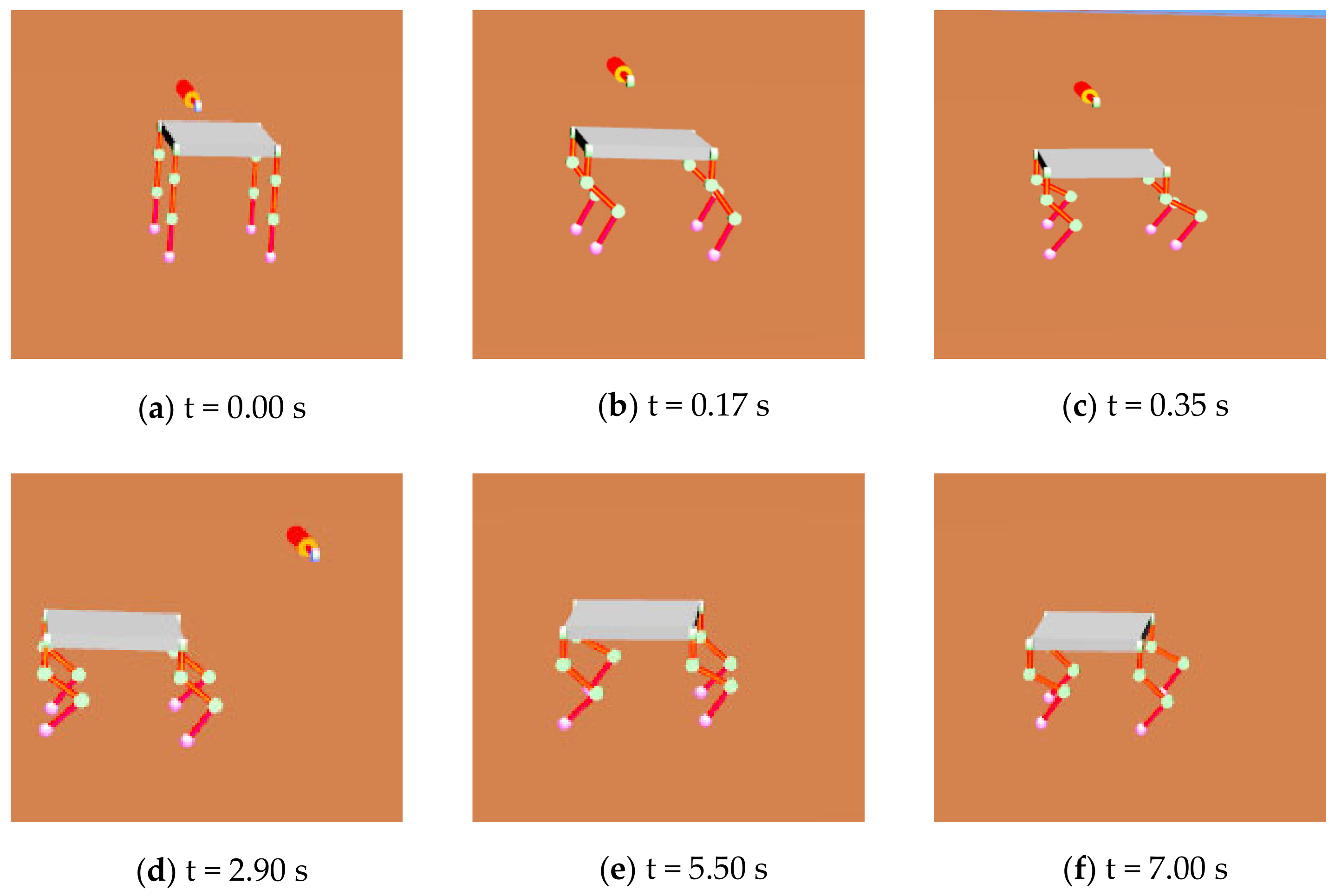
In this simulation, Formulas (4) and (5) are used to plan the foot trajectory of quadruped robot, the step length S and step height H are set as 0 mm, 40 mm. $k_1$ and $k_2$ in Formula (11) are set as 20, 20. $\epsilon$ is set as 0.95. The robot’s change process with the adjustment strategy is shown in Figure 12:

The varied curve of roll angle and pitch angle is shown in Figure 13:

As shown in Figure 12 and Figure 13, after the simulation starts, the quadruped robot moves in place. At the 5.5 s, we apply a lateral impulse of $0.7 \mathrm{kg}·\mathrm{m}/\mathrm{s}$ to the robot, the robot begins to self-adjust to steady state. In the case of no adjustment strategy, the robot was subjected to lateral impact at 5.5 s and recovered to stable gait at 8.8 s, requiring an adjustment time of 3.3 s, the maximum roll angle change is 21.9 degrees, and the maximum pitch angle change is 16.2 degrees, after the stable walking, the robot roll angle fluctuates between $-1.31°$ and $1.31°$, and the pitch angle fluctuates between $-1.11°$ and $1.11°$. In the case of the adjustment strategy, the robot was subjected to lateral impact at 5.5 s and recovered to stable gait at 7.3 s, requiring an adjustment time of 1.8 s, the maximum roll angle change is 18.2 degrees, and the maximum pitch angle change is 9.2 degrees, after the stable walking, the robot roll angle fluctuates between $-0.92°$ and $0.91°$, and the pitch angle fluctuates between $-0.81°$ and $0.80°$. It can be concluded that when the robot is subjected to lateral impact, the addition of adjustment strategy can effectively suppress the substantial shaking of the body, the attitude angle changes little, and the body recovers stable faster.

5. Conclusions

Aiming at the balance control problem of quadruped robots, the main contribution of this paper is to propose a dynamic gait balance control method that adjusts the landing point through attitude feedback. To verify the effectiveness of the proposed adjustment strategy, we analyze the kinematics of the quadruped robot, design a reasonable gait, and then add the proposed strategy to the diagonal motion.

In the simulation environment, we carried out simulation verification in two scenarios of flat ground walking and lateral impact, respectively. By comparing the roll angle and pitch angle of the quadruped robot with and without the adjustment strategy, the effectiveness of the proposed method in adjusting the gait balance of the quadruped robot is verified. Simulation results show that this adjustment strategy can effectively suppress the fuselage shaking and enhance the fuselage stability in various scenarios.

However, in the face of more complex terrain, the balance adjustment effect of this method is not very good. To make the robot have better environmental adaptability, only relying on foot planning is not enough, more sensors need to be added to obtain ground information. Therefore, the next step is to apply perceptual information in gait planning to achieve balance control of the robot on more complex terrain.

References

- Playter, R.; Buehler, M.; Raibert, M. BigDog, Unmanned Systems Technology VIII. Int. Soc. Opt. Photonics 2006, 6230, 896–901. [Google Scholar]
- Raibert, M.; Blankespoor, K.; Nelson, G.; Playter, R. BigDog, the rough-terrain quadruped robot. IFAC Proc. Vol. 2008, 41, 10822–10825. [Google Scholar] [CrossRef] [Green Version]
- Sparrow, R. Kicking a robot dog. In Proceedings of the 2016 11th ACM/IEEE International Conference on Human-Robot Interaction (HRI), Christchurch, New Zealand, 7–10 March 2016; p. 229. [Google Scholar]
- Ackerman, E. Boston dynamics’ SpotMini is all electric, agile, and has a capable face-arm. IEEE Spectr. 2016, 6, 356–358. [Google Scholar]
- Hutter, M.; Gehring, C.; Jud, D.; Lauber, A.; Dario Bellicoso, C.; Tsounis, V.; Hwangbo, J.; Bodie, K.; Fankhauser, P.; Bloesch, B.; et al. Anymal—A highly mobile and dynamic quadrupedal robot. In Proceedings of the 2016 IEEE/RSJ International Conference on Intelligent Robots and Systems (IROS), Daejeon, Korea, 9–14 October 2016; pp. 38–44. [Google Scholar]
- Yang, W.; Yang, C.; Chen, Y.; Xu, L. Simulation of exoskeleton ZMP during walking for balance control. In Proceedings of the 2018 IEEE 9th International Conference on Mechanical and Intelligent Manufacturing Technologies (ICMIMT), Cape Town, South Africa, 10–13 February 2018; pp. 172–176. [Google Scholar]
- Folgheraiter, M.; Yessaly, A.; Kaliyev, G.; Yskak, A.; Yessirkepov, S.; Oleinikov, A.; Gini, G. Computational efficient balance control for a lightweight biped robot with sensor based ZMP estimation. In Proceedings of the 2018 IEEE-RAS 18th International Conference on Humanoid Robots (Humanoids), Beijing, China, 6–9 November 2018; pp. 232–237. [Google Scholar]
- Yuan, S.; Zhou, Y.; Luo, C. Crawling gait planning based on foot trajectory optimization for quadruped robot. In Proceedings of the 2019 IEEE International Conference on Mechatronics and Automation (ICMA), Tianjin, China, 4–7 August 2019; pp. 1490–1495. [Google Scholar]
- Chen, G.; Hou, B.; Guo, S.; Wang, J. Dynamic balance and trajectory tracking control of quadruped robots based on virtual model control. In Proceedings of the 2020 39th Chinese Control Conference (CCC), Shenyang, China, 27–29 July 2020; pp. 3771–3776. [Google Scholar]
- Chen, G.; Guo, S.; Hou, B.; Wang, J. Virtual Model Control for Quadruped Robots. IEEE Access 2020, 8, 140736–140751. [Google Scholar] [CrossRef]
- Zhao, J.B.; Ma, S.; Niu, S.; Wang, J. Fractional-order virtual model control for trotting motion of quadruped robot. In Proceedings of the 2020 Chinese Control and Decision Conference (CCDC), Shenyang, China, 22–24 August 2020; pp. 4935–4942. [Google Scholar]
- Xie, J.; Ma, H.; Wei, Q.; An, H.; Su, B. Adaptive walking on slope of quadruped robot based on CPG. In Proceedings of the 2019 2nd World Conference on Mechanical Engineering and Intelligent Manufacturing (WCMEIM), Dalian, China, 29–31 October 2019; pp. 487–493. [Google Scholar]
- Shang, L.; Li, Z.; Wang, W.; Yi, J. Smooth gait transition based on CPG network for a quadruped robot. In Proceedings of the 2019 IEEE/ASME International Conference on Advanced Intelligent Mechatronics (AIM), Hong Kong, China, 8–12 July 2019; pp. 358–363. [Google Scholar]
- Pelit, M.M.; Chang, J.; Takano, R.; Yamakita, M. Bipedal walking based on improved spring loaded inverted pendulum model with swing leg (SLIP-SL). In Proceedings of the 2020 IEEE/ASME International Conference on Advanced Intelligent Mechatronics (AIM), Hokkaido, Japan, 6–10 July 2020; pp. 72–77. [Google Scholar]
- Shan, K.; Yu, H.; Gao, H.; Zhang, L.; Deng, Z. Stance phase leg actuation control of the active SLIP running based on virtual constraint in sagittal plane. In Proceedings of the 2018 Annual American Control Conference (ACC), Milwaukee, WI, USA, 27–29 June 2018; pp. 1969–1974. [Google Scholar]
- Meng, X.; Yu, Z.; Huang, G.; Chen, X.; Qi, W.; Huang, Q.; Su, B. Walking control of biped robots on uneven terrains based on SLIP model. In Proceedings of the 2019 IEEE International Conference on Advanced Robotics and its Social Impacts (ARSO), Beijing, China, 31 October–2 November 2019; pp. 174–179. [Google Scholar]
- Vukobratović, M.; Borovac, B. Zero-Moment Point—Thirty Five Years of Its Life. Int. J. Hum. Robot. 2004, 1, 157–173. [Google Scholar] [CrossRef]
- Raibert, M.H.; Chepponis, M.; Brown, H.B. Running on four legs as though they were one. IEEE J. Robot. Autom. 1986, 2, 70–82. [Google Scholar] [CrossRef] [Green Version]
- Raibert, M.H. Trotting, pacing and bounding by a quadruped robot. J. Biomech. 1990, 23, 79–98. [Google Scholar] [CrossRef]
- Won, M.; Kang, T.H.; Chung, W.K. Gait planning for quadruped robot based on dynamic stability: Landing accordance ratio. Intell. Serv. Robot. 2009, 2, 105–112. [Google Scholar] [CrossRef]
Figure 1.
Billy robot dog simplified structural model.
Figure 2.
The single-leg model of the quadruped robot is modeled by the D-H method.
Figure 3.
Virtual leg equivalent model of the quadruped robot.
Figure 4.
The soar period of the actual diagonal gait.
Figure 5.
The robot attitude feedback is displayed from different perspectives. In (a), it’s a view from the positive to the negative direction of the y axis. In (b), it’s a view from the positive to the negative direction of the x axis.
Figure 6.
Four cases of gravity center distribution. In (a), the gravity center is before the 2–3 diagonal. In (b), the gravity center is behind the 2–3 diagonal. In (c), the gravity center is before the 1–4 diagonal. In (d), the gravity center is behind the 1–4 diagonal.
Figure 7.
Robot gravity center adjustment.
Figure 8.
Gait adjustment strategy flowchart.
Figure 9.
A simulation of the quadruped robot in Webots.
Figure 10.
Simulation process of the quadruped robot walking on flat ground after adjustment strategy is added. In the beginning, the robot is in the air 50 mm away from the ground, and each joint of the robot is in position 0.
Figure 11.
The quadruped robot walks on flat ground. In (a), the roll angle curves of the robot without and with the adjustment strategy are compared. In (b), the pitch angle curves of the robot without and with the adjustment strategy are compared.
Figure 12.
Simulation process of quadruped robot subjected to lateral impact. At the beginning, the robot does step movements.
Figure 13.
Lateral impact is applied to the quadruped robot as it moves in place. In (a), the roll angle curves of the robot without and with the adjustment strategy are compared. In (b), the pitch angle curves of the robot without and with the adjustment strategy are compared.