PSciLab: An Unified Distributed and Parallel Software Framework for Data Analysis, Simulation and Machine Learning—Design Practice, Software Architecture, and User Experience

Abstract

In this paper, a hybrid distributed-parallel cluster software framework for heterogeneous computer networks is introduced that supports simulation, data analysis, and machine learning (ML), using widely available JavaScript virtual machines (VM) and web browsers to accommodate the working load. This work addresses parallelism, primarily on a control-path level and partially on a data-path level, targeting different classes of numerical problems that can be either data-partitioned or replicated. These are composed of a set of interacting worker processes that can be easily parallelized or distributed, e.g., for large-scale multi-element simulation or ML. Their suitability and scalability for static and dynamic problems are experimentally investigated regarding the proposed multi-process and communication architecture, as well as data management using customized SQL databases with network access. The framework consists of a set of tools and libraries, mainly the WorkBook (processed by a web browser) and the WorkShell (processed by node.js). It can be seen that the proposed distributed-parallel multi-process approach, with a dedicated set of inter-process communication methods (message- and shared-memory-based), scales up efficiently according to problem size and the number of processes. Finally, it is demonstrated that this JavaScript-based approach for exploiting parallelism can be used easily by any typical numerical programmer or data analyst and does not require any special knowledge about parallel and distributed systems and their interaction. The study is also focused on VM processing.

1. Introduction

Any numerical computation can be composed of a set of interacting functions. One form of this is a linear sequence of functions, but often, computational functions can be divided into sets of parallel function evaluations. There are two classes of partitioned numerical computation:

• Strongly coupled, with extensive data dependencies and communication interaction;
• Loosely coupled, with a low degree of inter-function data dependencies and communication.

Statistical data analysis, simulation, and machine learning are typical examples of computational problems that belong to the second class and can be easily processed by parallel and/or distributed computational processes. The focus of this work is on the second class of problems.

A heterogeneous cluster-based parallel and distributed numerical and machine learning framework is introduced using the widely available JavaScript Virtual Machines (VM), either as part of a web browser (client-side) or as part of a dedicated server-side engine (e.g., node.js). It features an easy and explicitly controlled way to compose parallel and distributed numerical computation, via worker processes that can be created and processed on a wide range of platforms and accessed and controlled by a web browser (laboratory in the Browser). The parallelization of numerical tasks has been under investigation for more than 60 years. This work addresses the practical aspects and explores the problem space suitable for parallelization and distribution.

This work provides no new theoretical contributions to parallel and distributed systems. Instead, this work proposes a unified software framework for hybrid distributed–parallel computation, with a rigorous experimental evaluation of the performance of parallel and distributed data-processing systems, exploring typical numerical scenarios and using consumer hardware including smartphones and widely available software like web browsers. This paper identifies optimized software and architecture details, suitable metrics by which to assess computational nodes in advance, and the classes of problems that are suitable for our proposed and implemented multi-process and communication architecture with a focus on VM technologies.

Primarily, parallel and network-connected hierarchically organized distributed-parallel data processing systems will be addressed that use web browsers (WorkBook software) and command-line shells using node.js (WorkShell software) deployed in heterogeneous environments. Code can be executed independently of the underlying host platform and the programs. Program code can be processed on both architecture classes, mostly without code modification. Both architecture classes can be coupled via communication channels. The novel Parallel Scientific Laboratory (PSciLab) software framework bundles a set of tools and modules to create numerical multi-processing using common JavaScript virtual machines (VM). This framework is a conceptual successor of the original PsiLAB framework using the OCaml VM [1]. PsiLAB was limited to single-process execution and used native code libraries to perform computationally intensive operations (like matrix BLAS or FFT packages). In addition, the PSciLab software framework does not rely mostly on any native numerical code library supporting web browser processing.

The first goal of this work is related to processing architectures and an investigation of the suitability of low-cost hardware (i.e., mainly consumer electronics with integrated Intel CPU and GPU architectures, smartphones, and embedded computers) with respect to distributed and parallel scaling and overall performance. There is a focus on hybrid distributed-parallel systems combining parallel and distributed computing that is coupled closely. Finally, the benefits of integrated low-cost GPUs are evaluated. The second goal of this paper is related to the deployment of virtual machines (VM) using JavaScript programming in heterogeneous networks. JavaScript has the advantage of being widely used, and JS can be executed on any machine. Using Google’s V8 core engine (part of the Chrome web browser and node.js), native code performance can be reached. The easy-to-learn and easy-to-use JS-based parallel data-processing framework (e.g., distributed ML requires fewer than 500 lines of code) is the main advantage of this framework over other frameworks like Python or TensorFlow, for example. The usage of web browsers simplifies its operation since no software installation is required. In contrast to Jupiter notebooks interfacing a separated Python VM, for instance, the WorkBook is self-contained and performs all computations.

Two scenarios addressing large-scale multi-entity simulation and multi-model ML are used to demonstrate the capabilities of this software architecture and programming environment.

An overview of the PSciLab software framework and its components is shown in Figure 1. This software framework enables hybrid and hierarchical parallel and distributed processing using the following components:

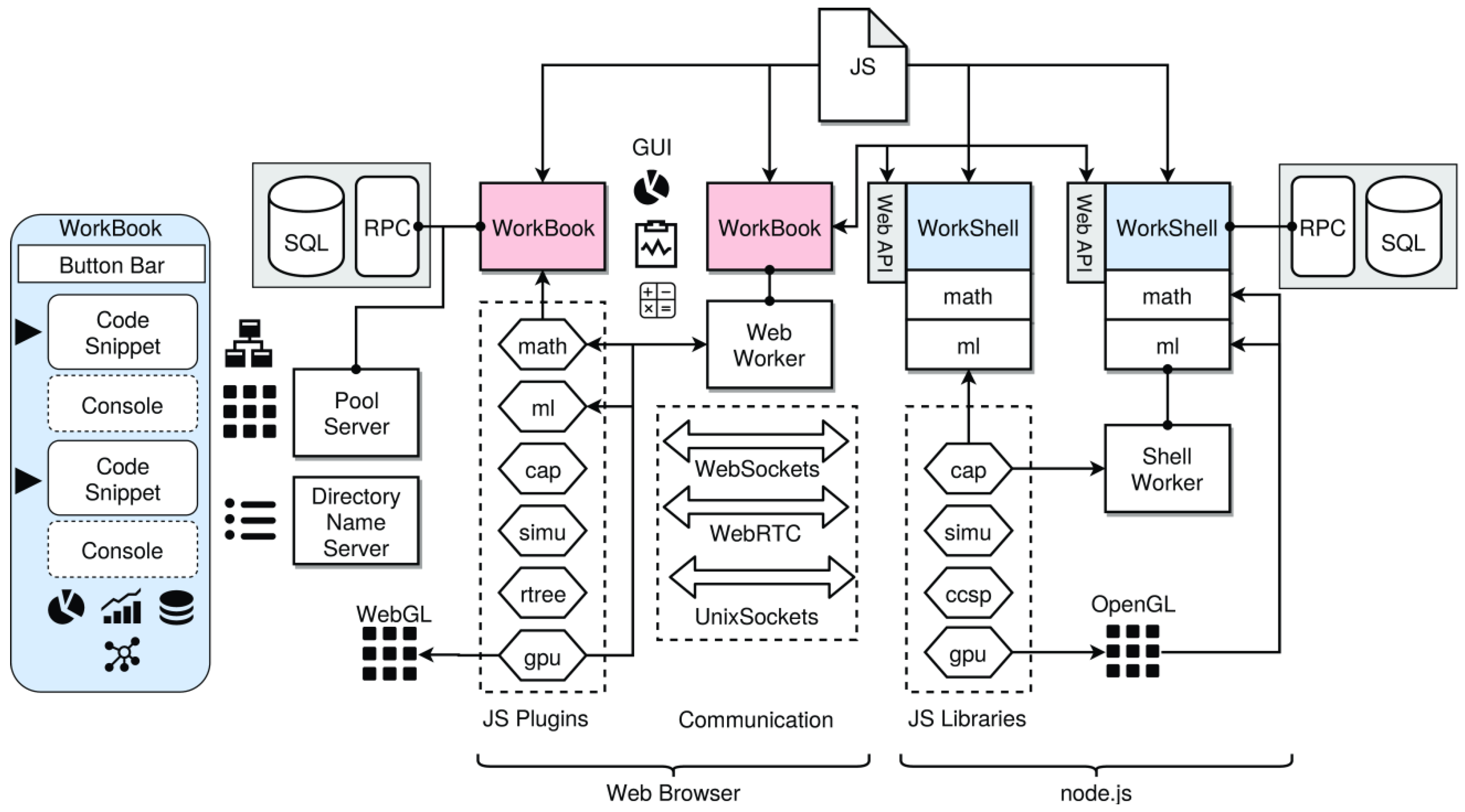
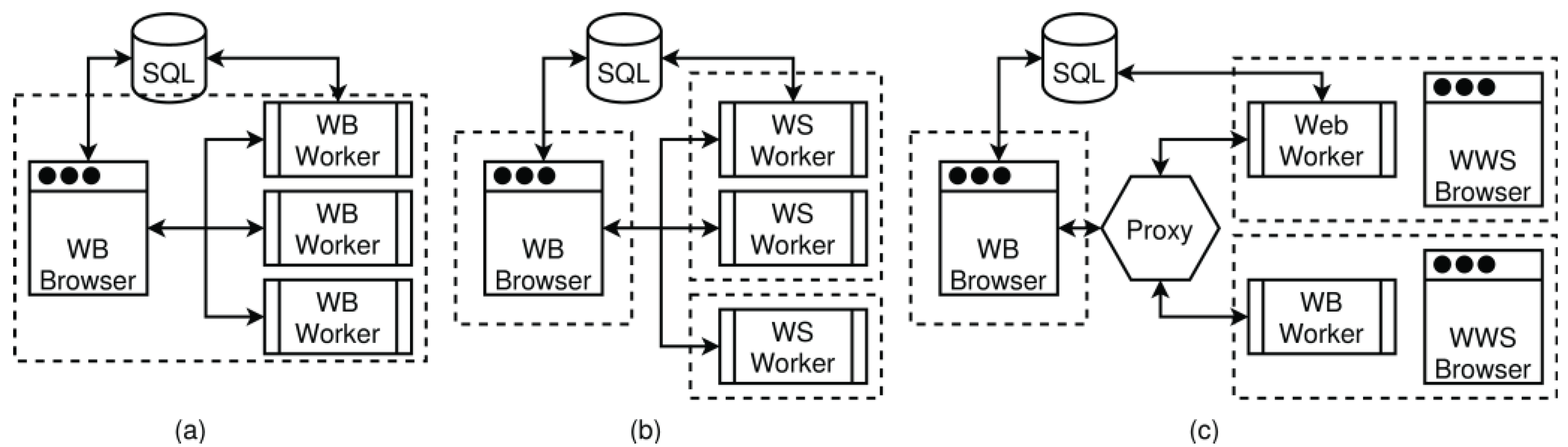
• WorkBook: The first main software component is the WorkBook, processed by a web browser that provides a Graphical User Interface (GUI), including extensive graphical data visualization, like data plotting with code snippet workflows similar to, e.g., MatLab or the Jupiter Notebook. A WorkBook can be used as a standalone or together with WorkShells (or other WorkBooks). A WorkBook can spawn either web workers to perform computational tasks locally in parallel or shell workers for distributed computing. Scripts executed via workers (web and shell) started from a WorkBook can execute visualization operations directly.
• WorkShell: The second main component is a headless and terminal-based WorkShell that is processed by node.js [2] and can be accessed directly by WorkBooks. The WorkShell can be used as a standalone (executing scripts from a command line) or used together with WorkBooks provided by a web service Application Programming Interface (API). A WorkShell can spawn system workers to perform computational tasks in parallel.
• SQLite: The third main component is a set of (distributed) customized SQLite databases, with remote network access services via a JSON-based remote procedure call (RPC) interface used for input, intermediate, and output data exchange.
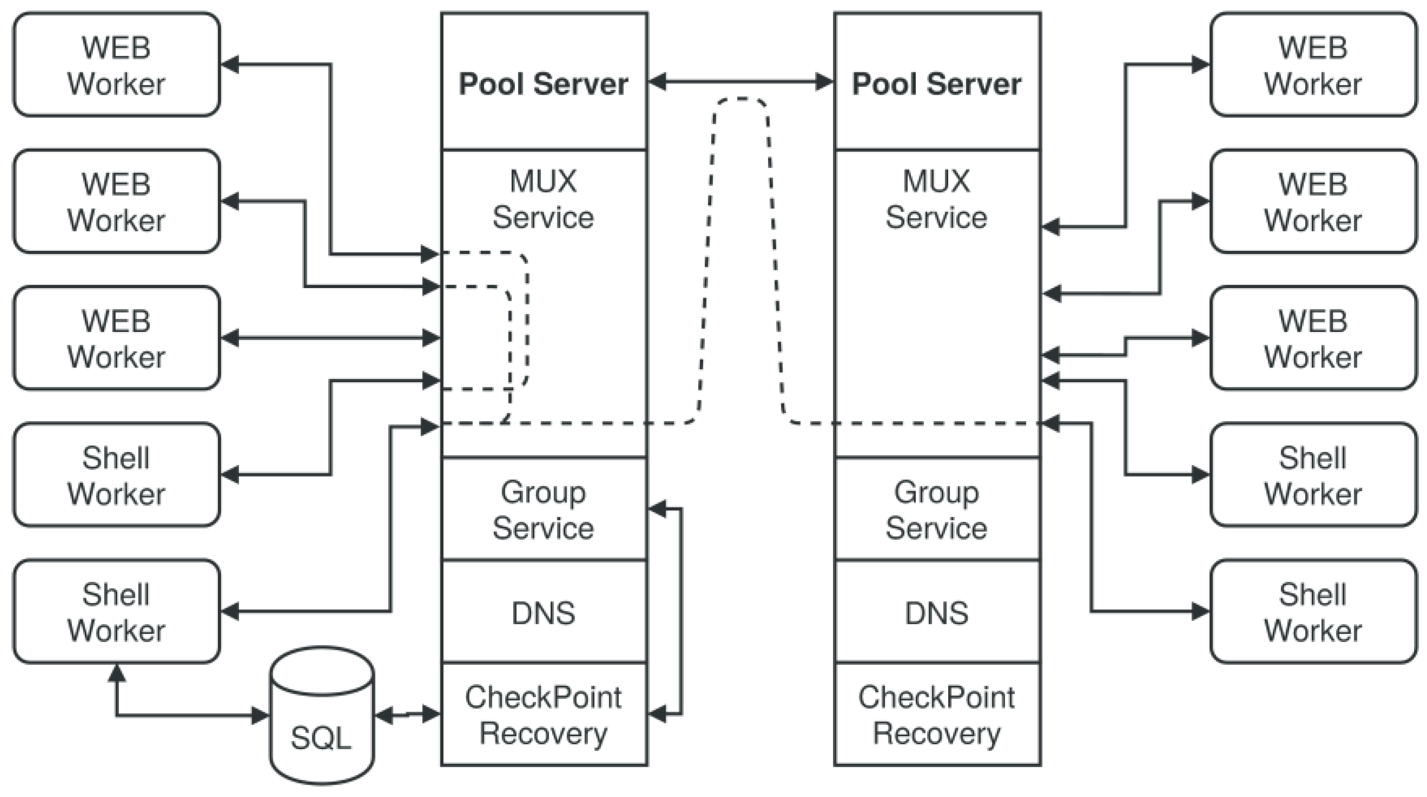
• Pool/Proxy: An optional worker pool server and Internet proxy for connecting workers (WorkBooks and WorkShells, along with their worker processes) and providing a group service.

The entire framework, as well as the user code, is programmed entirely in JavaScript, ensuring high portability. Additionally, there is a web WorkShell component providing a web-based WorkShell (with a terminal console) for web browsers, extended with a sub-set of the WorkBook and common libraries. The Web WorkShell (WWS) can be integrated into any web page. The WWS can be configured by URL parameters, including script loading. It is mainly used for participative crowd computing. Finally, the interconnectivity of computational processes among the Internet is provided by a pool and proxy server via WebSocket communication.

The following sections introduce the fundamentals of multi-processing architecture, data management, the parallel and distributed programming of workers, and the software framework itself. Finally, an extended case study section evaluates the benefits of the PSciLab processing framework for two prominent applications. It is clear that VM-based computation can compete with native approaches and there is a suitable speeding- and scaling-up model that can be achieved by worker groups.

The novelty of this framework is its high portability and the support of strong heterogeneous networks of computers, the web browser as a scientific laboratory, tight scaling to large-scale problems, the void of special software or hardware components, and the ease of programming without expert knowledge (regarding parallel and distributed systems). Hierarchical parallel-distributed clusters are supported seamlessly using a unique API.

2. Related Work

The computational performance of modern computer systems originally developed rapidly, with almost exponential growth in operational speed and memory. In the past decade, however, there has been stagnation. The memory capacity was still doubling almost every year, but the operational throughput (computational powers) was nearly constant. However, the demand for computation currently doubles every three months, mostly driven by ML and data-mining tasks. Parallel computation as applied to numerical problems is a long-existing field of computer science. Originally, it started with networked computer clusters in the 1960s (clusters of workstations), then came the rise of dedicated parallel computers in the 1980s, and finally the advent of cloud computing, using distributed server farms appearing as one virtual machine. With the rise of multi-core computers, consumer software, and commonly used numerical software like MatLab [3], developers have tried to exploit parallelism. Parallel computation is generally used to reduce the computational time by vertical (sub-tasks applied to the partitions of input data) and horizontal (pipelines applied to different input data) parallel processing. However, control-path and data-path parallelism need to be distinguished. Control-path parallelism can be created easily by multiple worker processes executed on different machines (clusters) or CPUs (cores). Data-path parallelism can only be achieved with dedicated hardware (although CPUs support VLIW extensions) by field-programmable gate arrays (FPGA) or customized ASICs, today mostly performing general-purpose computing tasks on graphical processing units (GPGPU), but this is primarily still fine-grained control-path parallelism or hybrid approaches [4].

Two different dominant parameters were identified in [3] that have a significant impact on the speed of parallel systems: (1) the memory model (shared memory vs. distributed memory, memory architecture, cache hierarchy, bandwidth, etc.); (2) the granularity of the parallel tasks on a data- and control-path level, as well as the parallel execution time, compared with the overhead (setup and communication). For example, the start-up time of a JS VM using WorkShell code can consume up to one second (see Section 8.1 for details). The third, less dominant parameter is the communication load and communication architecture. Communication introduces synchronization, and synchronization introduces temporal sequential processing that reduces the degree of parallelism that can be achieved.

With the rise of the internet and the web, high-bandwidth networks and powerful web-browser software capable of executing JavaScript efficiently via server-less computation using an interconnected web browser were successfully deployed for numerical computations [5]. The web browser as a computational node is also a central part of the current work. The JS VM is the key methodology and technology for cluster computations in heterogeneous environments. JS is always passed to the VM in an architecture-independent text format (UTF8 code) and can easily be exchanged. Moreover, any JS object and even functions can be serialized into text by the JavaScript object notation (JSON) format and again deserialized into code or data objects. Besides core data types like numbers and strings, JSON supports only non-nested record data structures and polymorphic arrays. An extended version, JSONfn, is used in this work using a modified serializer and deserializer that also encodes functions, typed arrays, matrix objects, and generic data buffers. By using web browsers, peer-to-peer communication can be realized by WebRTC [5] or by using a proxy server and WebSockets. WebSockets are an upgrade of an HTTP(S) connection that requires an external HTTP service, whereas WebRTC depends on external signaling (STUN) and relay (TURN) servers. WebRTC data channels enable direct browser–browser (and browser–server) communication. However, the symmetric network address translation (NAT) prevents direct IP-UDP-based communication and requires a relay server. For this reason, and because of the non-availability of WebRTC data channels in web workers, WebSockets, and generic HHTP requests, together with an external proxy server, are used in this work only. Generic single HTTP requests (GET/PUT methods) are preferred for remote procedure calls (RPC), whereas WebSocket channels are primarily used for data and control streams.

Messaging and communication architectures were identified early as a central limiting factor with respect to achievable speeding- and scaling up as a function of problem size that has to be addressed by suitable communication models [6]. Algorithms and structures of parallel programs have to be adopted carefully to benefit substantially from parallel processing [7]. There is no universal parallel computer and communication architecture that matches all problems and algorithms efficiently. The parallel simulation of large-scale multi-entity systems (e.g., multi-agent systems or cellular automata) is one major scenario that is addressed by parallel and distributed computation [6,8]. Parallel cellular automata (PCA), used to compute or simulate complex systems, are still under development, e.g., in materials science and micro-structure simulation [9] or for image processing [10]. Spatial domain partitioning is commonly applied to the cell grid to achieve a parallel decomposition of this computational problem. In [11], load-balancing and CPU allocation are identified as key challenges in the parallel and distributed computation of CA. In this work, a pool server is introduced that is capable of managing computational groups and worker processes on demand (computation as a service architecture).

Besides micro-scale simulations, macro-scale simulations, like urban simulations (traffic, migration, segregation, energy supply, etc.) or pandemic simulations that involve a high number of cells or entities, are demanding for parallel and distributed computation due to their high computational complexity [12] and complex long-range communication graphs. An agent-based simulation is another field of parallel computation [13], in contrast to cellular automata (CA), with short-range entity–entity communication (data dependency) that is suitable for parallel decomposition, with nearly linear scaling in terms of the problem size and number of processors. Multi-agent systems can be characterized by long-range communication, limiting the scaling up and achievable speeding-up significantly and limiting the efficient distribution of computation, but domain-specific partition and communication restrictions can relax this limitation. The first case study evaluated in this paper applies spatial world partitioning for the parallel processing of a CA. A partitioning scheme commonly relies on a shared or distributed memory model. Simulation including Multi-agent Systems (MAS) can exploit data-path (shared-memory) parallelism, using GPGPU acceleration and control-path parallelism with network clusters equally [13]. The hardware acceleration of agent-based simulation, using GPGPU and accelerated processing units (APU), is still an ongoing research field [14].

The second major field today demanding parallel computation is data-driven modeling, using machine learning (ML) methods and high-dimensional data analysis. In contrast to multi-entity simulation with a spatial context, enabling parallel decomposition on a control-path level, ML generally requires data-path parallelism with a high-bandwidth shared memory architecture to achieve reasonable speeding- and scaling up. However, multi-model, ensemble and distributed ML can benefit from control-path parallelism, even when using low-resource devices with low computational power and memory storage [15]. The second case study evaluated in this work is multi-model training for parallel hyper-parameter space exploration. In [16], the authors discuss JavaScript-based artificial neural network software frameworks and the suitability of web browsers for ML tasks. They conclude that web browsers can compete with native code server-based frameworks like TensorFlow.

There are only a few systems using large-scale artificial neural networks (deep ANN) partitioned over several nodes, as discussed in [17,18], and there are communication limitations preventing efficient control-path parallelism for the training of smaller network sizes (fewer than 100,000 parameter variables). Most of the current systems do not split the ANN itself and each physical computing node handles the entire ANN [19]. Instead, data-path parallelization is achieved by GPU (e.g., CUDA API with the cuDNN library [20]) and FPGA accelerators. Cloud computing, e.g., using the Hadoop framework based on map and reduce methodologies, is increasingly used for large model sizes. The decomposition of a large predictive model into a forest of smaller partial models (e.g., in a multi-class classification problem where each model is a single-class predictor, trained stochastically [17]) with model fusion is a suitable methodology for distributed training with a low communication overhead.

Some common parallel and distributed programming and communication environments include the parallel virtual machine (PVM), recently extended to heterogeneous systems, including CPU/GPU hybrid systems [21], and the message passing interface (MPI) [22]. Both frameworks require expert knowledge for the efficient design of distributed-parallel systems.

The architecture of data input-output streams, as part of the communication infrastructure of parallel and distributed systems, has a significant impact on scaling- and speeding up. Memory-in-place methodologies are only suitable for parallel systems using shared memory architectures. Distributed memory should be organized and the communication overhead must be considered carefully. Databases can provide the necessary organization of data. In this work, a set of relational SQL databases is used; however, SQL databases do not scale linearly with increasing data volume and complexity. It is difficult to distribute the partial content of databases. Typically, NoSQL databases are chosen for large-scale cloud computing and data-mining tasks [23]. Temporal databases are suitable for the processing of latent temporal data streams and large amounts of temporary data. The SQL database was chosen here because of its lightweight implementation, SQLite, which can be embedded efficiently in any application program, even in a web browser using transpiling technologies. SQLite provides an advanced cache algorithm that reduces file access significantly in distributed computations like multi-model ML (reading the same input data multiple times).

3. Problem Formalization and Taxonomy

The taxonomy of parallel and distributed applications is related to data and application classes, e.g.,

• Data classes: vector, matrix, tensor, functional data (cellular automata);
• Algorithm classes: matrix operations in general, data-driven and iterative optimization problems, cellular automata processing, simulation, equation-solving, regression, statistical analysis;
• Data dependency classes: local, global, clustered, static and dynamic content, static and dynamic sizes, and horizontal (time) and vertical dependencies;
• Processing flow classes: data flow ⇔ functional flow, control flow ⇒ synchronization;
• Partitioning classes: single-data and single-model vs. multi-data and multi-model computation (e.g., ensemble model ML with model fusion, data streams);
• Model classes: data-driven modeling, e.g., using ML methodologies, split into training, test, and validation phases, hypothesis tests and model selection (parallel model space exploration), hyper-parameter space exploration;
• Size classes: static size vs. dynamic size problems.

3.1. Data Classes

The following data class taxonomy is addressed by any numerical software framework:

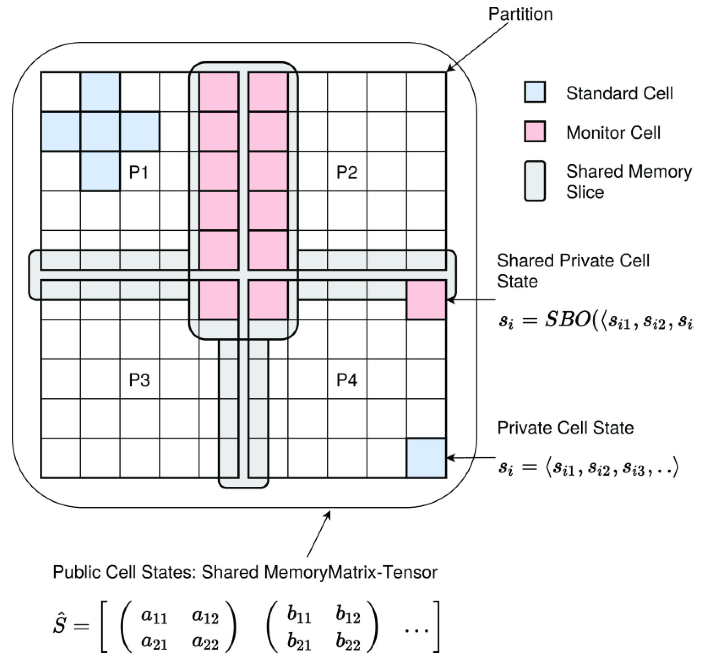
• Data Dimension. Matrix (and vector) operations rely on multiply-add and loop instructions that require fine-grained parallelism on a data-path level. If independent matrix segmentation is possible with respect to input and output data, then coarse-grained parallelism on the control path can be partially applied. Cellular automata with a grid world are examples of the deployment of control-path parallelism.
• Data Sets. If there is an unordered data set D^~ = {d_i}_i consisting of independent data items, then these data items can be processed independently and in parallel, i.e., d₁ → f¹ || d₂ → f² || …, where f^j are replicated functions derived from a master f.
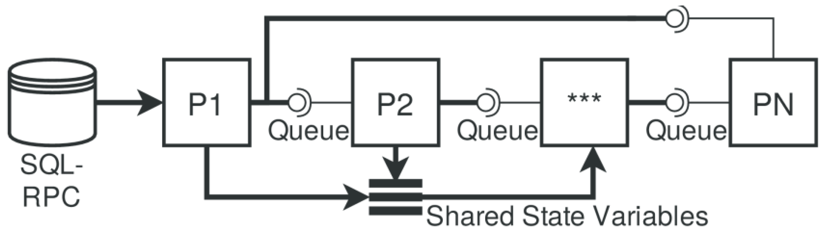
• Data Streams. If there is an ordered sequential data stream D^~ = [*d*_t]_t consisting of independent data items provided in a sequential stream, and there is a functional chain f₁ → f₂ → … → f_n, vertical control-path level parallelism can be exploited efficiently in a functional chain, i.e., d_j → f_i || d_j+1 → f_i−1 || d_j+2 → f_i−2 and so on. Functional pipelines can be used to exploit functional-level parallelism on a horizontal control-path level.
• Model Sets. If there is a non-unique and non-deterministic optimization problem using data sets, e.g., ML, i.e., M^~ = {m_i}_i, then control-path level parallelism (multi-processing) can be used to derive the set of models M^~ from the same data set (or any sub-set) but with a different parameter variable set (including random variables), i.e., f¹(D,p₁) → m₁ || f²(D,p₂) → m₂ || … || fⁿ(D,p_n) → m_n, where f^j are replicated functions derived from a master f.

Data sets can be distributed on different computers and can be classified into two different fragmentation classes [24]:

• Horizontal Fragmentation. There are sub-sets of instances that are stored at different computing nodes N^~ = {N_i}_i, i.e., D^~ = {d_i}_i, d₁ → N₁, d₂ → N₂, …, d_n → N_n.
• Vertical Fragmentation. There are sub-sets of attributes (variables) of instances that are stored at different sites.

Data set fragmentation is an important feature that is exploited by our parallel and distributed data processing framework.

3.2. Problem Classes

There are two different problem classes with respect to the computational size (number of instructions) and data size (number of data elements):

• Static. The problem size is static, i.e., |D| = s = const, and does not change with parallelization, i.e., by increasing the number of processing nodes N_i and processes P_j(N_i). Static-sized problems are well suited for partition, as in grid-based simulation (CA), i.e., the full data set is partitioned and processed on multiple nodes (different data on different nodes): D = {d_i}_i, d₁ → f¹ || d₂ → f² || … || d₂ → f^k. The aim of parallelization is the reduction of overall computation time, ideally by 1/PN if PN is the number of parallel processes.
• Dynamic. The problem size grows with an increasing number of processing nodes and computational processes. An example is multi-model ML training. Each processing node trains an independent model with different parameter variables from the set V = {v_i}_i, including random variables (Monte Carlo simulation), either using the same input data D or different input data D₁, …, D_u, or sub-sets d_i ∈ D, i.e.: ⟨D,v₁⟩ → f¹, …, ⟨D,v_n⟩ → fⁿ. The aim of parallelization is ideally a constant computational time, with an increasing number of parallel processes (scaling is S = 1), or at least, growth lower than PN = |P|, i.e., 1 < S < PN.

The presented software framework addresses both problem-size classes. Two case studies will be given to demonstrate each problem class.

3.3. Algorithmic Classes

In this work, primarily, control-path parallelism is addressed. This constraint requires the capability of algorithms to be partitioned into tasks with low (or medium) data interdependency and low inter-task communication (i.e., synchronization). Although shared memory communication is supported, the communication overhead should be kept low to achieve a nearly linear scaling with the number of processors (in the range of 4–100). Some prominent examples satisfying this constraint are certain machine learning applications and large-scale multi-entity simulations. If the input and output data can be partitioned into independent data sub-sets, then this criterion can be met immediately.

3.4. Machine Learning

Data-driven machine learning (ML) can profit from two parallelism methods:

• Data-path parallelism. This is applied to function evaluation and matrix operations.
• Control-path parallelism. This is applied to the training of multiple models (multi-instance ensemble learning and/or parameter space exploration) or to inferences in multiple data sets and/or multiple model instances.

ML can be further classified into a taxonomy similar to Flynn’s computer architecture, but here it uses model instances for training (deduction) and inference (induction):

• STSI. Single-model instance training with single-model instance inference (i.e., 1:1 mapping of input and output data to models); input and output data is not partitioned;
• MTSI. Multi-model instance training with single-model instance inference, either by model and parameter space exploration selecting the best model or by model fusion; input and output data is not partitioned;
• MTMI. Multi-model instance training with multi-model instance inference, i.e., primarily distributed ML; input and output data is partitioned and single model instances operate only on a (local) sub-set of the input data; final global model fusion is optional;
• STMI. Single-model instance training with multi-model instance inference, e.g., pixel-based feature detection being applied to images or replications of the trained model; input data for training is not partitioned, input data for inference data can be partitioned.

ML is typically a minimization problem repeatedly iterating over a set of data instances. A single ML task itself has no inter-process data dependencies during the training and inference phases. ML can therefore profit from pure control-path parallelism and distribution, but the parallelization of one training task poses high inter-layer data dependency and communication and, therefore, can only profit from data-path parallelism (e.g., used by Tensorflow with a GPU back-end) applied to matrix operations. The input training and test data only need to be transferred once and the communication time can usually be neglected (compared with the training task). The iterative optimization process that minimizes an error/loss function by parameter adaptation uses the same input data repeatedly. Generally, there is a forward pass that computes the model with the given input data, finally applying the loss function to compute the error, followed by a backward pass that adjusts the model parameters, based on that error. Artificial Neural Networks (ANN) and function regression are prominent models that are trained by forward-backward propagation algorithms. This allows efficient parallel computation on the same node (including outsourced GPGPU computations) as well as distributed computation on different independent computing nodes for multi-model training.

3.5. Simulation

Large-scale multi-entity simulation is a computationally intensive task. An entity is either passive, like a volume in the finite element methods (FEM) used for physical and mechanical simulations, or active, either as a simple state-based Turing machine (a state-based finite state machine (FSM)) in a cell of a cellular automata (CA) system or a more complex agent in a multi-agent system (MAS). FEM and CA cells present short-range interaction leading to static short-range (local) data dependencies (and data exchange), whereas agents can offer short- and long-range interaction up to global data dependencies and global communication. That is, FEM/CA cells have a fixed set of neighboring elements, whereas agents have dynamic sets of interacting agents. This is important for parallelization and the distribution of simulations.

Control-path parallelism can be efficiently applied to multi-entity simulation if there is either a regular geometrical ordering of the elements or if it is possible to partition the geometrical cell space Σ in mostly independent sub-partitions and regions {σ₁, σ₂, …}, ideally with a 1:1 mapping of partitions on worker processes [8]. Both FEM and CA worlds can be partitioned into independent areas. MAS simulations can be partitioned in the same way, based on agent context and with geospatial constraints limiting the communication (mostly) of agents to the bounds of a geospatial region, e.g., the social interaction of agents is limited to the current spatial context (building spaces are independent of street areas, and so on).

Each sub-partition σ_i containing a number n of entities can primarily use private memory for the state variables of the entities. Only boundary entities close to another sub-partition/region require shared memory or message-based communication, implementing distributed memory. The first case study in this paper will discuss a sliced memory architecture with shared and non-shared memory segments.

The distributed simulation requires message-passing that produces a significant overhead and can affect scaling up and speeding up. A hybrid distributed-parallel approach can be used as a good trade-off, i.e., parallel simulation on the same host platform using shared memory, with distribution on multiple host platforms (clustering).

3.6. Virtual Machines

Many numerical software frameworks rely on native code execution. That is, there is a set of native code libraries that performs numerical operations like matrix operations or signal transformation. Some frameworks, like Tensorflow for solving ML tasks, support different software front-ends (e.g., Python) and hardware back-ends (e.g., CPU and GPU), creating a significant overhead. This approach typically provides optimal performance with respect to computation time and working memory allocation. Some software frameworks utilize parallel exploitation. For local deployment, this can be sufficient, for a distributed system, this can be a showstopper. Depending on the computer architecture, the byte order of numerical data formats can differ in a heterogeneous computational cluster, preventing the direct exchange of numerical (and other object) data. Additionally, native code frameworks can lead to code dependency problems (like the non-matching API of system libraries). Compiling from source code is not always an alternative solution (as in the R framework). The Microsoft and Apple OS frameworks do not ship with code compilers.

These limitations can be overcome by the deployment of virtual machines and by using widely available script languages. Code execution is mostly or always performed directly from device-independent text code that is typically compiled into Bytecode on the fly (and on-demand). Python is a prominent example, but the Bytecode VM is one of the slowest VMs (1:100 compared with V8/node.js). JavaScript (JS) is another widely used scriptable programming language. A script differs from traditional complete (compiled) software in that there is no start-up and main code to be provided, but, in contrast to Python, JS can be efficiently parsed (v8/Spidermonkey: more than 1 M lines/second), compiled, and processed by advanced VM technologies, such as just-in-time (JIT) native code compilation. Google’s V8 engine is a prominent example, achieving nearly native code performance. Even pure Bytecode engines like Spidermonkey provide sufficient performance to perform numerical data processing, including simulation and data-driven modeling with ML (see the case study section for examples).

The main advantage of text-scriptable VMs over traditionally compiled native code processing is automatic memory management by a garbage collector (GC). However, GC-based memory management demonstrates two significant drawbacks: (1) memory allocation—the memory release of unused objects occupies significant computation time that is not available for real numerical computation (overhead); (2) the automatic memory release is lazy and there is theoretically a higher average memory consumption than in user/program-controlled software. In practice, manual memory management leads to memory leaks and memory errors, but the first issue is most relevant when assessing the computational power of VM-driven data processing. Finally, VMs prevent the exploitation of parallelization. Automatic memory management and GC mostly prevent the sharing of the program state by multiple VM instances, although there has been progress in parallelizing VMs. The node.js platform prevents multi-threaded processing for some time; it is still a multi-threaded VM but it just has a set of full and independent but coupled VM instances. The start-up time and the overall memory footprint are oversized. These constraints must be considered carefully if parallel and distributed systems are composed using a VM like node.js. Fine-grained parallelism cannot be exploited efficiently.

4. Multiprocessing: Models and Architectures

4.1. Processes and Composition

This work primarily addresses control-path parallelism, although data-path parallelism using GPU co-processors and the general-purpose programming of GPUs can also be exploited. Basic data processing is executed by a sequential process, performing computation within a specific data context (scope). That is, the computational system consists of a set of sequential processes P_seq = {p_i}_i=1,n that are processed in a given order that is either control- or data-driven. In numerical and machine-learning tasks, the single computational processes are data-dependent and are typically chained, i.e., from a functional view, addressing the data flow F(x): x → p_n(p_n−1(…p₁(x)))) → y, and from a process algebraic view, addressing the control flow: P = p₁→p₂→…→p_n. The sequential processes p_i are typically assigned to the sub-tasks of numerical computation, known in this work as code snippets. Each process p is processed in a private data and code context, exchanging data with other processes via global variables or data queues. Each process can be in one of five control states: {START, RUN, END, AWAIT, BACKGROUND}. A process is started either implicitly or explicitly, resulting in the control-state transitions START → RUN. At any time, the process can pause for the satisfaction of an event condition, e.g., waiting for the completion of a communication action, resulting in the process transition RUN → AWAIT → RUN. Process flows with synchronized process chaining can be created by defining input and output data dependencies with implicit data queues, or by using explicit process control statements.

The multi-process model is close to the concurrent communicating processes model (CCSP), originally introduced by C. Hoare and widely used in multi-threading and multi-processing. Each process is executed independently, typically by an independent VM instance and ideally by its own CPU (core). Synchronization is provided by message passing or shared memory. Concurrency is resolved by mutual exclusion locks (either implicitly or explicitly).

JavaScript is strictly sequentially processed without pre-emption, but the control flow can be suspended by using promise handlers and the await statement inside asynchronous functions, for example:

async function sleep(tmo) {
  return new Promise(function (resolve) {
    setTimeout(resolve,tmo)
   })
}
async function serviceloop() {
  for(;;) {
    // service 
    await sleep(1000)
   }
}
serviceloop()
		

Multiple asynchronous functions can be started, then suspended by the “await” statement, with the sequential scheduling of other waiting but ready asynchronous functions (with promises satisfied by the previous call of the resolver function). However, there is no parallel processing of asynchronous functions (except low-level IO tasks under the hood).

The horizontal sub-task data dependency in the functional chain prevents parallel processing of these computational processes, which are associated with the functions. However, chained data processing systems can be executed by a pipeline approach that executes the computational processes in parallel with different chained data, i.e., there is a parallel process system Par({p_i}_i=1,n) = p₁ || p₂ || … || p_n with a set of inter-process synchronization using channels c connecting the processes C = {c_i:p_i → p_j}_i=1,m. This approach requires an ordered data set sequence D = {d(i)} and is only applicable to data streams (otherwise, no efficient utilization of the different processors can be achieved). Both vertical, as well as horizontal, pipelined processing is supported by the WorkBook and WorkShell software platforms.

The JS VM does not provide any programmatical parallelization; there is only one main control-flow, even by using “asynchronous” callback functions, Although IO behind the wall is processed as multi-threaded, using asynchronous functions with the concept of promises and the “await” operation enables control-flow scheduling, which is important in message-based and synchronized multi-process systems. There may be more than one suspended function call in progress that can introduce ambiguous behavior with multiple background suspended-code snippets. To prevent hidden asynchronous function executions, WorkBook and WorkShell provide cancellation operations.

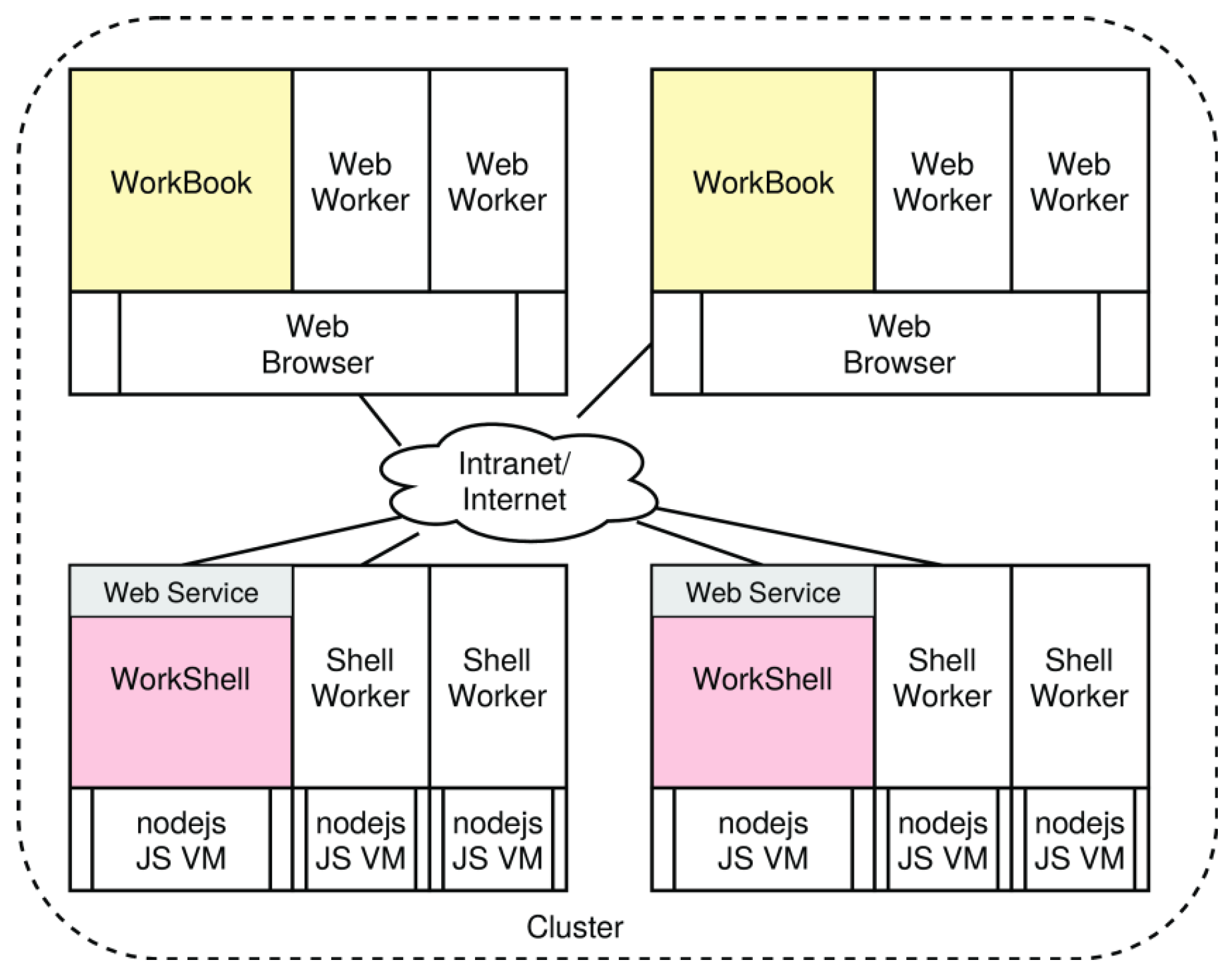
4.2. Hierarchical Processing Architecture

This software framework combines the distributed and parallel composition of large-scale systems in strong heterogeneous environments, as shown in Figure 2.

4.3. Process Classes

From the technical point of view, there are two different worker process classes:

• Web browser (WorkBook) processing JavaScript via V8 or SpiderMonkey VMs and providing a dynamic Document Object Model (DOM):
  • The main process (master execution and control loop);
  • Lightweight WebWorker processes (executed by OS threads, controlled by the main process) with a reduced sub-set of the WorkBook (providing control-path parallelism);
  • WebGL-based GPGPU kernel processes (providing data-path parallelism).
• Node.js (WorkShell) processing JavaScript by the V8 VM:
  • The main process;
  • Separate worker processes executed by independent and isolated OS processes, with a full WorkShell code base (providing control-path parallelism);
  • OpenGL-based GPGPU kernel processes (providing data-path parallelism).

All processes are executed by independent JS VM instances, and local and remote worker processes can be mixed. Inter-process communication (IPC) is provided for the unidirectional master-worker (functional data messages), unidirectional worker-master, bidirectional worker-master process RPC communication using virtual channels, and worker-worker communication via shared memory-based queues. It is assumed that a computational node n_i ∈ N is capable of processing multiple processes in parallel (multi-core and/or multi-CPU architectures). Note that GPU utilization is typically limited to one process per node and GPU.

4.4. Worker

A worker process can be created with only a few lines of program code in a Workbook or on a (remote) WorkShell, either directly or via the WorkShell Web API service, shown in Example 1 for shell workers and created from a Web WorkBook remotely. There is a unified wrapper-class Worker that covers both WorkBook and WorkShell workers, as well as local and remote workers. The worker object instantiated from the Worker class provides full control over the worker process. The worker object can finally be used to execute code in the worker process.

var workers=[]
// Creation of local Web or Shell workers
// Worker is child process of this parent process 
var worker = await new Worker(id?,{options});
await worker.ready();
workers.push(worker)
// Creation of remote workers
// On cpu42 machine start: worksh -p 5104:protkey 
var workers =  []
for(var i=0;i<NUMWORKERS;i++) {
  var shellworker = await new Worker(’ws://cpu42:5104’,i,{options}); 
 
  await shellworker.ready();
  workers.push(shellworker);
}
		

• Example 1. Creation of local and remote web and shell workers via the unified “Worker” class. Shell workers can be created remotely via the ShellWorker web API.

After workers are created, they can be accessed programmatically by executing code or by evaluating functions, as shown in Example 2. The data state between successive function calls is preserved, i.e., functions can be state-based, reusing data from previous function executions.

// asynchronous execution without reply 
for(var i=0;i<NUMWORKERS;i++) {
  workers[i].run(
   function (i) {
     var result = compute(i);
     send(result)
   },
   i);
}
// join and collect 
for(var i=0;i<NUMWORKERS;i++) {
  results.push(await workers[i].receive())
}
// synchronous execution waiting for results 
for(var i=0;i<NUMWORKERS;i++) {
  var result = await
    workers[i].eval(
      function (x) { return 1/(1+Math.exp(-x)) },
      Math.random());
}

• Example 2. Execution of functional code on (web or shell) workers (following Example 1).

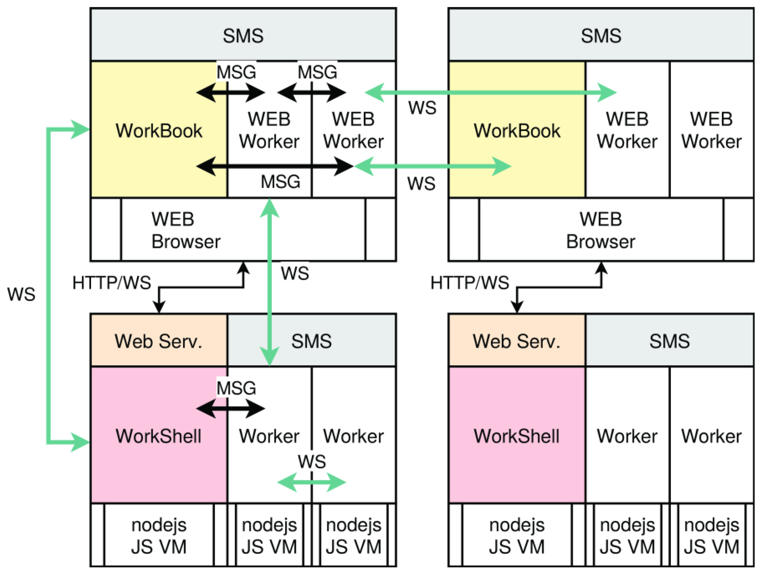
4.5. Communication, Synchronization, and Data Sharing

Processes (either the WorkBook or WorkShell main loop, and web or shell worker) can communicate and synchronize by using either message-based communication M or shared memory S, as shown in Figure 3:

• Native messages M_native provided by the browser or by the node.js platform; these can only be used within the same process class and by a parent-worker process group on the same node → synchronization and data transport.
• WebSocket messages M_ws can be used between all process classes and different nodes → Synchronization and data transport.
• Shared memory segments S_sms (SMS), implemented either with shared array-buffers in the browser or with native externally mapped shared memory at system-level in node.js; these can only be used within the same process class and on the same node → data sharing without data-driven synchronization.
• Shared buffer objects (BO) S_smo are implemented in SMS with static typing, supporting atomic core variables, structure variables, and arrays → data sharing without data-driven synchronization.
• A shared matrix S_sma implemented by shared memory and object-wrapper replications; these can only be used within the same process class → data sharing without data-driven synchronization.
• Queued and synchronized data channels M_ch built on native streams, Unix or WebSocket messaging, using (1/2), or shared memory (4).
• Remote procedure calls over message channels.

A combination of M and S methods can be used for efficient inter-process communication in typical numerical, simulation, and machine learning tasks.

Bidirectional master–worker communication is performed by message-based channels, using send and receive operations on message channels. Additionally, a worker process can perform asynchronous (event streams) to synchronous remote procedure calls in the master process. Worker–worker synchronization (limited to the same worker class and the same host) can be established with Atomics-based operations on shared array buffers, implementing the following IPC objects:

• Mutex;
• Semaphore;
• Barrier;
• Data Queues.

Local workers (instantiated from the same parent process) communicate via UNIX sockets or data pipes. Remote workers (or those not instantiated from the same parent process) communicate via HTTP WebSocket (WS) channels. The protocol overhead of TCP-based WS channels is relatively low (except for the upgrade protocol), being below 5–10% depending on the payload size per message transfer, as shown in

Table 1. Communication overhead for TCP-WebSocket channels by sending serialized matrix data (initialized with random numbers) between a shell worker and a WorkBook. The raw network RX-TX data load was measured by and collected from the LAN device. Overhead factor OF in parenthesis: pure payload.

Host	Matrix	Data (Bytes) ×N	RXTX (Bytes)	OF
HPG3-WS/CFLX3-WB	2 × 2	(30 + 80) × 500,000	66,309,928	1.21 (1.65)
HPG3-WS/CFLX3-WB	10 × 10	(30 + 1955) × 20,000	42,468,779	1.07 (1.09)
HPG3-WS/CFLX3-WB	1000 × 100	(30 + 1,929,253) × 20	40,784,371	1.06 (1.06)

. The constant message overhead (JSON format) is always 30 Bytes. In the case of very small payload data, the overhead increases (about 20% for 80 bytes/message, or 65% if considering the pure payload only). The advantage of WS channels over other more efficient protocols is the capability to connect web browser processes with remote shell-worker processes (and by using a proxy server for web worker–web worker communication). This is a key feature for the deployment of distributed heterogeneous systems. A theoretical discussion of the protocol overhead of WebSocket connections can be found in [25]. Examples of bandwidth and message latency measurements for local worker process communication (typically via UNIX sockets or pipes) are shown in

Table 2. Communication latency τ and bandwidth BW for local-worker communication using channels by sending serialized matrix data (initialized with random numbers) between a worker and the main process.

Host	Matrix	Data (Bytes)	N	τ (ms/msg)	BW (MB/s)
CFLX3-FF52-WB	2 × 2	81	50,000	0.37	0.21
CFLX3-FF52-WB	10 × 10	1943	10,000	0.47	3.9
CFLX3-FF52-WB	100 × 100	192,880	1000	8.3	22.2
CFLX6-CR90-WB	2 × 2	81	50,000	0.01	7.0
CFLX6-CR90-WB	10 × 10	1945	10,000	0.02	110
CFLX6-CR90-WB	100 × 100	192,929	10,000	0.42	450
CFLX3-WS	2 × 2	80	50,000	0.018	4.2
CFLX3-WS	10 × 10	1950	10,000	0.08	23.5
CFLX3-WS	100 × 100	192,919	1000	1.44	127.8
HPG3-WS	2 × 2	81	1,000,000	0.005	15.4
HPG3-WS	10 × 10	1945	1,000,000	0.024	78.1
HPG3-WS	100 × 100	19,2864	10,000	1.3	141.1

. The node.js platform provides low-latency and high-bandwidth communication. The current Chromium browsers offer very high bandwidth and very low latency for master–worker communication.

Channel- and stream-based WebSocket communication relies on a state-based connection using TCP between both communication endpoints. That is, any temporary network failure or transmission disturbance can result in a permanent disconnect of the communication channel. A WebSocket channel is provided by an upgrade process over an HTTP(S) connection. After a disconnect, this upgrade has to be performed again. This state-based communication is a limiting factor in the design of distributed systems and in the access of remote-worker processes. Shell workers created via the WorkShell Web service are automatically terminated if there is a disconnect from the master process (e.g., a WorkBook session). All data and computation of this worker are lost permanently. To overcome this limitation, there are three solutions:

• Using state- and connectionless communication via UDP/WebRTC;
• Workers (or the WorkerShell Web service) can be kind and tolerate temporary connection loss, and wait for a reconnect;
• A persistent snapshot by check-pointing the worker state using secondary storage.

Solution (1) is not suitable for distributed systems. The communication channels are used for master–worker synchronization. UDP is not reliable; there is no information if the other communication endpoint is still alive and, therefore, synchronization over such unreliable channels is not free from deadlocks and there is no starvation freedom. Solution (2) shifts the problem only temporarily, but this is the most suitable method, while solution (3) results in high communication overhead. Moreover, the state of a JS execution context cannot be dumped fully (free variables cannot be resolved programmatically), but long-running tasks should explicitly dump their intermediate results to enable the reincarnation of a crashed worker process. For example, in ML training, the iteratively trained model is serialized and is saved periodically. Our distributed SQL data base can be a valuable storage point. At any particular moment, this time-consuming training process can be restarted from the last snapshot.

Finally, Example 3 shows some WorkBook/WorkShell operations to perform synchronous master-worker communication and synchronous RPC execution.

  // Create worker with RPC 
  var worker = new Worker({
    rpc : {
      function foo (x) { return x*x }
    }
  })
  // In worker process 
  var ma = Math.Matrix.Random(10,10),
     mas = serialize(ma.data);
  send(mas)
  var mat = deserialize(await receive())
  var result = await rpc.foo(2);
  // In parent process 
 
  var data = await worker.receive()
  var matrix = deserialize(data)
  matrix.transpose()
  worker.send(serialize(matrix))
		

• Example 3. Master–worker communication using message channels or RPC.

The interprocess communication shown above is mainly used by parent–child process groups. Totally independent worker processes can communicate via a proxy server, as discussed in Section 4.8, creating ad hoc groups.

4.6. Security

As in any distributed system, there must be some level of access protection. This addresses the accessing of data storage (in this framework, SQL data bases with RPC service) and the access and creation of worker processes on remote machines. Typical approaches with user-related authentication and authorization are a major barrier in the implementation of heterogeneous and scalable parallel and distributed computational systems. User and authentication servers are required.

The services provided by the PSciLab software framework instead use capability-based access control methodologies. A capability consists of four parts:

• A public service port assigning the capability to a specific service, but not a specific host;
• An optional object number of the service (e.g., a specific data base or processor);
• A rights field that specifies the allowed operations of the services (e.g., reading or writing data bases);
• A security port that contains the encrypted rights field by using a private port.

A capability is not bound to a specific user or host computer. A capability is therefore transferable. A directory name service (DNS) can be used to map names onto capabilities. The private port to encrypt the rights field is handled by the service and is kept secret.

4.7. Pipelines

Single-code snippets can also be considered as processes. Connecting them enables pipeline processing, as shown in Figure 4. Code snippet processes can perform computation independently from other snippets, reading input data from input channel queues, writing output data to output channel queues, and using shared-state variables. In principle, code snippet processes can be processed by different processors (either web or shell workers) as long as they exchange data via the channel queues.

The queued channel network enables synchronized in-order processing of data. Besides data exchange via channels (functional data flow), there are shared state variables that can be used by code-block snippets to access data out of order.

4.8. Pool Server and Working Groups

The pool server consists of a group of services via HTTP(S) messages, a WebSocket proxy service with a virtual circuit multiplexer (connecting groups of worker processes), and a worker management service.

The start-up time of a worker process varies between 50 and 1000 ms and depends on the worker class (browser or shell), the host platform architecture, and the OS (see Section 8.1). Worker processes can be created and started in advance. In this case, each worker process provides an RPC service loop that can be used for control, data exchange, and code snippet execution (REPL) by a master process (or another worker). However, the state of the worker process is persistent and cannot be reset, i.e., a worker process should not be reused for different jobs scheduled by different master processes. In contrast, worker tree clusters consist of a main process (WorkBook or WorkShell). This main process can spawn an arbitrary number of worker processes from the same class (local, i.e., web worker or WorkShell instances) or from another class (local or remote). Each Workbook and WorkShell main instance provides a worker service that can be used to create workers.

There is a set of main master processes running in the WorkBook in a web browser that are started by a WorkShell and executed by node.js. WorkShell provides a web service that enables worker creation by remote programs (assuming that they have sufficient capabilities to perform this operation). The master process or an already spawned worker process can execute code on workers.

Worker processes can be grouped in pools controlled by a pool manager server (PMS), as shown in Figure 5. The PMS can be accessed via web sockets from any host, including web browser applications. The PMS acts as a router that can dynamically connect worker processes that have already started with each other and with the main process at run-time, providing a virtual communication channel (VC) multiplexer. Two instance-levels of PMS registration are provided: (1) top-level instances capable of creating new workers; (2) worker instances (already created or created on-demand).

This group and pool management provides a registration service for the WorkShell and WorkBook main control processes and worker processes. It performs the load balancing of worker pools on new worker creation requests (process migration is not supported) or creates workers on registered WorkShells. Instead of contacting the WorkShell web API proxy service directly (although this is still possible and useful), the pool server is responsible for selecting the appropriate pool nodes, based on static and dynamic statistical parameters (e.g., the number of current worker sessions, lazy load evaluation, and computational and storage metrics). The major measure of the computational power of a computing node is measured with a dhrystone benchmark (a JS version processed by the node.js or Browser VM, see Section 8.1 for examples). The case study evaluation section will show that the dhrystone benchmark is suitable for predicting normalized computational times. A second parameter shows the number of CPUs and CPU cores of a physical node and, finally, the total working memory storage capacity. A 1:1 mapping of worker processes to CPUs or CPU cores per physical node should be met. The pool server tries to create and allocate worker processes in groups. That is, a client can request a number of grouped worker processes at once, with a specific computational power and estimated memory storage requirements. The request can constrain the worker selection based on equal CPU measures, to ensure that there is no slow worker process that suspends the fast worker processes of the group to the idle state (a 100% load is aimed for).

WorkShell or WorkBook nodes can be added or removed at any time. Note that only WorkShell can provide a remote Web service for worker creation (accessed remotely, directly, or via the pool/group services). Web WorkBooks can spawn worker processes but cannot directly grant access to remote workers. The web workers can only be accessed via the pool/group service.

A distributed set of PMS connected with fully meshed message channels provides suitable scaling-up for large-scale distributed systems. The PMS cluster handles different physical computing nodes and services independently but negotiates worker process trading by group communication.

Load balancing in heterogeneous node clusters is important to optimize total computation times. The nodes can vary in terms of computational power and memory capacity. The relative computation power, measured in dhrystones, can be used to partition computational tasks on nodes. For instance, in multi-model ML, there can be models with different numbers of parameters (neural nodes) and model structures. Smaller models can be processed by slower nodes, larger models by faster nodes, still creating a significant speeding-up or preserving a constant time-scaling.

Independent worker processes can create ad hoc working groups by using the proxy and group service of the pool server. Groups can be created at runtime, and a worker process can join a group and ask for other members of the group. Each peer process is identified by a unique number and connects to the proxy service via WebSocket channels. A worker process connected to the proxy can be connected with any other connected worker process (by virtual circuit channels). An example is shown below.

var gs = group.client(url,{});
var socket = await gs.connect();
gs.create(‘myworkinggroup1’);
... // wait for other members joining the group 
var members = await gs.ask(‘myworkinggroup1’)
// connect this peer port with other member ports 
for (var i in members ) {
  if (members[i]==socket.peerid) continue;
  await socket.connect(members[i],true /*bidir*/)
}
socket.write({cmd:‘eval’,f:function (x) { return x*x},
           x:Math.random(),from:socket.peerid})
var result = await socket.read();
		

• Example 4. Direct worker group programming using the proxy and group service.

4.9. Worker Process Control

Worker processes are created and controlled programmatically at run-time. There is no pre-defined multi-processing network. Code snippets or functions can be executed on a worker process either by the WorkBook code snippets, with a pragma code line pointing the execution to the desired (spawned) worker directly, or programmatically, by code processing functions sending the code to the worker processes and, typically, waiting for the termination or an evaluation result. A worker preserves its data state between code snippet executions. Although web workers are created by the browser, native workers created by a shell script, and shell worker processes created remotely are handled by different modules, there is one unified top-level function Worker that is used to create worker processes, independent of their location and host and returns a process control object.

        // Local Web or Shell Worker
worker = new Worker(id?,options?);
        //  Remote WorkerShell Service 
        new Worker(‘shellhost:port:capability’,options?);
        // Remote Proxy Service 
        new Worker(‘proxyhost:port:capability’,options?);
await worker.ready()
await worker.run(‘data={x:1,y:2}; function foo(x) { return x*x }’);
result = await worker.eval(‘return foo(100)’);
result = await worker.evalf(function (x) return foo(x-1) },100);
data = await worker.monitor(‘data’);
print(data.x)
worker.kill();
		

• Example 5. Typical snippet for worker creation (internally, with web workers, on a remote WorkShell, and by using the pool/group server proxy service).

5. IO Data Management and Data Sharing

5.1. Distributed SQL Databases with RPC

Central to any parallel and distributed system is transparent data organization, storage, and access, using a unified data storage and query interface. In our system architecture, a distributed SQL data base with a remote procedure call (RPC) access service and JSON data transfer for remote access is used to store input, intermediate, and output data in a unified way. Among flat tables, hierarchical data tables and data sets are supported. Finally, the SQL data base service supports virtual tables, providing a mapping of local files on tables, e.g., a CSV table stored in a file, a “numpy” matrix, or a set of image data files. The size of the data files is not limited, and clients can access the tables, sliced row-wise. The SQL data base serves as an exchange platform for parallel computational processes. The main advantage of a remote distributed data management system is the capability to access data independent of the process location and processing environment, typically limiting distribution and parallelization in a heterogeneous model, like the one found in this work.

The SQL database consists of the following components:

• A native SQLite3 module for the node.js platform.
• A JavaScript interface module that creates SQLite3 data base instances and provides programmatical access to a data base.
• A JavaScript JSON service API, mapping JSON requests to SQL statements and vice versa.
• A JavaScript RPC service via HTTP/HTTPS or WebSockets, providing JSON-formatted SQL queries and some additional operations. An extended JSON format is used to support functional requests with a function code. The function code consists of state-based micro-operations applied to the SQL data base that are used to compose complex operations. Access can be secured by a capability-based right-key authorization mechanism.
• A file-mapper module that provides virtual SQL tables from data files, e.g., image files can be accessed as raw or converted matrix data, with meta-information organized as rows in SQL tables.

The data base can be stored in a single file on disk or held temporarily in the memory. A data base and tables in data bases can be created or deleted by any worker process, regardless of their physical and logical position (if the worker provides sufficient capability rights). The memory data bases play an important role in the worker–worker data exchange of intermediate computation results. Any data type can be stored in table columns, including serialized JavaScript arrays and records. Finally, this SQL server provides virtual access to data files that are mapped on SQL tables, e.g., a set of image files, a set of data matrix files in numerical Python format, and many more file formats are supported. Only a YAML metafile must be provided (along with the data files) that describes the mapping schema.

The SQL data bases are used for input, intermediate, and output data. In the case of ML, this includes the storage of serialized trained models, like neuronal networks. The SQL data base also provides a storage point for snapshots created by worker processes. A checkpoint with a snapshot contains all the data and information to restart a crashed worker process from its last state. An example of SQL-based check-pointing saving the relevant data state of a worker is shown below in Example 6.

// Create an ANN trainer 
var sql = DB.sql(‘ws://host:port:key’);
// Create a checkpoint tables for data state snapshots 
var cptable = ‘checkpoint-’+myGroupId+‘-’+myWorkerId
if (!options.checkpoint) {
  sql.create(cptable,
          { time:‘number’, iter:‘number’, err:‘number’,
            model : ‘blob’ })
  var model = ML.learner(ML.ML.ANN, { options })
} else {
  var row = sql.query(cptable,‘*’,‘rowid=’+options.checkpoint)
  var model = ML.deserialize(row[0].model);
}
while (i < maxIter || err > errThr) {
  var result = ML.train (model, data, { options });
  if (i>0 && (i % 4)==0) sql.insert(cptable,
    {time : time(), iter:i, err:result.error,
    model : ML.serialize(model) });
  i++; err=result.error;
}
send (ML.serializes(model))
// delete checkpoint table
sql.drop(cptable)
		

• Example 6. Worker check-pointing of the data state, enabling recovery.

5.1.1. Replicated Data Bases and Tables

Since a single SQL server is a critical central instance, preventing the appropriate scaling of parallel and distributed applications, the RPC-SQL API provides functions to copy entire tables by a single operation. Furthermore, those tables distributed on multiple SQL servers can be merged.

var sql1 = DB.sql(‘ws://hosta:porta:keya’),
sql2 = DB,sql(‘ws://hostb:portb:keyb’);
sql1.copy(‘tablename’,sql2)
		  

5.1.2. Capability Protection

The previously introduced capability mechanism is used to protect the SQL service, data bases, and, optionally, specific tables. The rights mask of the capability determines the allowed operations of the requesting worker process:

• Reading tables and table rows.
• Modifying tables and modifying rows.
• Creation and deletion of tables.
• Creation and deletion of data bases.

Alternatively, for the sake of simplicity and deployment in local networks, a simple string key can be provided that is always associated with the full rights mask.

5.1.3. Application Programming Interface

There is a unified data base module that can be used by any worker process to access remote data bases. The API provides one main function to create an access handle for a specific remote data base service by providing a valid URL with access capability. The access capability specifies the allowed operations on the data base. The handle provides functions to query the data base. A handle can switch between different data bases provided by the same service port, as shown in Example 7.

var sql = await DB.sql(url,options)
var databaseList = await sql.databases()
sql.open(‘mydatabase1’)
var tableList = await sql.tables()
await sql.create(‘mytable’,{$colname:$type})
await sql.insert(‘mytable’,{$colname:$data})
var rows = await sql.select(‘mytable’,colums:string,where:string)
await sql.createDatabase(‘mydatabase2’)
await sql.open(‘mydatabase2’)
await sql.create(‘mytable2’,{$colname:$type})
		  

• Example 7. Typical RPC-SQL access examples.

The RPC-SQL service provides access to multiple data bases via one network port. Assuming sufficient client capabilities, new data bases can also be created remotely by a single operation. The newly created or opened data base can either be served by the same network port service or by creating a new service with a different network port on the fly.

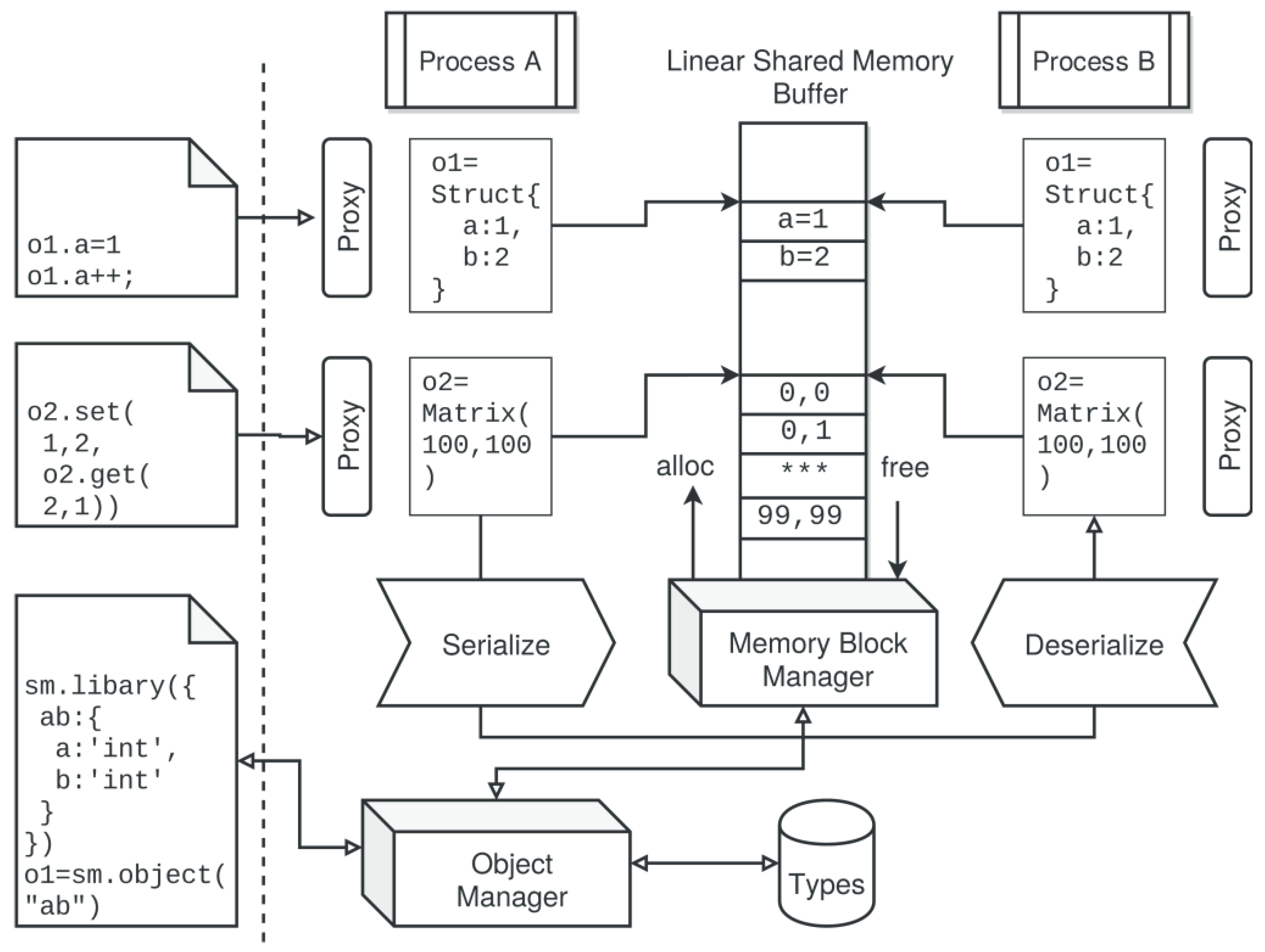
5.2. Shared Memory Segments and Buffer Objects

A shared memory segment (SMS) implements structured data with buffer objects (BO), creating shared buffer objects (SBO). The SMS provides linear memory management (linear memory block allocation and freeing), applied to the shared memory segment buffer. A buffer object is a proxy for scalar, array, or record-structured data. Each time a data element is accessed, the appropriate buffer handler operations transform high-level data access to low-level buffer operations, including the coding and decoding of data values with a linear memory model. SMS relies on “SharedArrayBuffer” objects in web workers and shared memory segments provided by the system-level OS in shell workers, respectively. A buffer object is stored in a region of the buffer segment that can be directly accessed by the high-level programming language via object monitors (proxies or getter/setter wrappers). Buffer objects are statically typified. Supported types are JS core data types (number, static strings, Boolean), C data size-constrained types (int8, int16, int32, float, double, …), composed record data types (records), mono-typed and static-sized linear arrays, and matrix objects based on linear typed arrays.

Finally, the SMS/BO implements shareable interprocess communication (IPC) objects, used for worker synchronization (on the same physical node):

• Mutex.
• Semaphore.
• Barrier.
• Data queue (synchronization via two semaphores).

The IPC objects use Atomics operations, applied to shared memory arrays (inside an SMS) to satisfy the inherent mutual exclusion. Shell worker processes (not worker threads) use named system-level semaphores instead.

There is a memory block manager that performs memory block allocation and release (low-level access to SMS), and an object manager that provides high-level access that supports object creation and destruction by using a type interface library or the programmatically provided type signatures of JS objects. The overall SBO architecture is shown in Figure 6. Any SBO can be serialized in one process and deserialized in another process (assuming that the SMS was already shared by the processes). This serialization creates an object descriptor containing memory and object information (like the type signature and object class).

SMS/BO are used by multiple worker processes to implement shared buffer objects (SBO) being accessed concurrently. These are used to share input, intermediate, and output data between worker processes of the same class (i.e., web worker or shell worker) and that are running on the same machine (host). The access to SBOs is not synchronized, although each basic read and write access of an SBO is atomic. In contrast to message-based communication, which is only directly possible between a worker and the main process, SBOs can be used for data communication between workers, although there is no synchronization. Programmatical access of SBOs is shown in Example 8.

// Create type interfaces 
var typesDef = {
  xy : { x:‘int’, y:‘int’, z:‘string’ }
}
// Create a generic shared memory buffer  
var sharedBuffer = new SharedArrayBuffer(1E5);
// Attach shared memory to SBS instance 
var sm=BufferSegment(sharedBuffer,{key:‘/shm1’});
sm.create();
// add type library
sm.library(typesDef);
// Create and initialize a shared object
objShared = sm.object(‘xy’);
objShared.x=0; objShared.y=0;
// Create workers 
var worker = new Worker(...)
// Share SMS 
await worker.share(‘this.sm1’,sm)
// Share Buffer Object 
await worker.share(‘this.objShared’,objShared)
// Shared typedarray matrix 
var matShared = sm.object(‘MatrixTA-Float32’,[1000,1000]);
matShared.set(1,1,Math.random())
await worker.share(‘this.matShared’,matShared)
// Access shared object in worker 
await worker.evalf(function (x) {
  this.objShared.x=x;
  this.matShared.set(1,2,
    this.matShared.get(2,1))},1)
// That’s all folks!
		

• Example 8. Creation and usage of a shared object memory with an initial set of object interfaces and one shared object.

Shared objects can be efficiently deployed if there is data interdependency between workers during computation. The access time of a shared object via the proxy monitor access (read/write) is only 2–10 times slower, compared with a native JS object. For example, in a web worker, the read or write access of a native JS object requires about 10 ns, whereas the access of a shared object (using SharedArrayBuffer objects) requires about 100 ns. In a shell worker using node.js, the native object access requires about 2 ns, whereas the shared object access (using OS-level named shared memory segments) requires about 4 ns. Matrix objects that use linear typed array (shared) buffers present similar access times. There is no significant difference in matrix cell access times (about 30 ns in a web-worker and 3 ns in a shell-worker process).

The SMS instance automatically manages the memory allocation and release of shared objects using the provided shared memory segment. The SMS method share provides the full logic to map the shared memory to the destination worker (dependent upon the worker class) and to create a copy of the SMS instance on the worker. Note that the “this” object is a persistent object in the top-level context scope of the worker and can be shared between successive worker calls.

5.3. Distributed Objects

Using object monitors and proxies, it is possible to distribute objects by message-passing. In contrast to the shared memory objects, an additional organizational layer is required to establish group communication. Distributed objects are not considered in this work or by the PSciLab software framework, but the framework can be extended with this feature.

5.4. Object Monitors

Similar to the concept of distributed objects providing synchronized read- and write access, object monitors enable the remote access of objects (worker A) via a message-based shadow object wrapper providing a seamless proxy (worker B or main process). An object monitor can be accessed via the programming language in the same way as the remote referenced object, e.g., by using element selectors for data structures or arrays (of numbers or structures). Although write operations are supported in principle, there is no synchronization or support for atomic operations. Object monitors are also supported for Web and shell workers.

// worker A
this.data = [1,2,3,4]
this.data[5]=5;
// main process 
var data = await workerA.monitor(’this.data’,1,false);
var sum = 0;
for(var i=0;i<data.length;i++) sum += await data[i];
		

6. Software Framework

The software framework consists of the following core components. Development snapshots can be downloaded from the github repository [26].

6.1. Parallel WorkBook

Parallelism is achieved by using Web Worker, message-based communication, and shared memory (including low-level IPC via shared memory). Unfortunately, since 2018, CPU bugs enabling adversarial memory leakage lead to disabling the shared memory in most major web browsers; hence, the usage of shared memory for fast worker–worker and main-worker IPC is limited to older browsers or requires a local or remote HTTP(S) server that can pass sufficient rights via COOP/COEP headers to the WorkBook to use shared memory.

6.2. Parallel WorkShell

The WorkShell is the command-line version of the WorkBook, processed by the node.js program. Node.js wraps the V8 core JS VM with asynchronous and multi-threaded IO loops. Most WorkBook script code can be directly executed in WorkShell and vice versa. Workers can be created by two methodologies:

• Process workers starting a new VM instance in a separate OS-level process, using message-based communication, and interprocessing shared memory segments on OS-level (memory mappings with native code, not controlled by JS VM).
• Thread Workers (available since node.js 10.5) starting a new VM instance in a thread, using message-based communication, and SharedArrayBuffers (memory that is shared by threads but controlled by the JS VMs).

6.3. Plugins and Libraries

There are a large number of plug-ins that can be loaded into a WorkBook (and web worker), including an extended mathematics plug-in. There are different matrix modules inside the mathematics plugin, representing a multi-dimensional matrix object with generic arrays or linear typed arrays. A matrix object wraps the data container with a large set of methods that can be applied to the matrix (or vector), including common matrix algebra. There is an extended unified ML plug-in that supports a wide range of ML models and algorithms, e.g., different kinds of decision trees, support vector machines, reinforcement learning, and artificial neural networks, including recurrent and convolutional networks. A GPU module can overlay matrix operations (part of the mathematics and ML library) with GPU-based replacements to speed up computations.

The mathematics and ML libraries are already integrated into the WorkShell program and are directly accessible by workers. The WorkShell can load additional libraries on demand. There is commonly a browser and a shell node.js version of a library.

6.4. Data Management

For data management, a customized SQLite server is used that is processed by node.js, as already discussed in Section 5.1.

6.5. Pool Management

Worker pools are managed by a pool/proxy/group server that is processed by node.js, as is already discussed in Section 4.8.

7. Data-Path Parallelism on GPU

Besides control-path parallelism, considered in the previous sections, in this section additional data-path parallelism is considered, performing general-purpose computation on graphics processor units (GPGPU) and the widely available WebGL/OpenGL API. Any computation that can be divided into independent data partitions, like matrix computations, can be processed by multiple GPU threads in parallel. However, GPU transpiled algorithms are not generally faster than the strict sequential code processed by the CPU. Most numerical frameworks (like Tensorflow) that support different CPU/GPU back-end packages either use CPU or GPU computing only. The overhead of GPU transpilation and the low sequential speed of the GPU processing elements can lead to speeding up below 1. GPU transpilation and code execution produce a significant overhead that is only justified if the real computation time (and, hence, the computational complexity) is sufficiently large compared to the overhead, including memory transfer and data code transformations. In this work, and in the PSciLab framework, dynamic CPU/GPU switching based on a priori and profiling information chooses the best back-end at run-time, according to complexity measures.

The dynamic switching (multiplexing) of computations between CPU and GPU, based on profiling, is eased by the fact that the GPU instruction code is derived from JavaScript kernel functions that are mostly equal to the Vanilla JS functions, except that the kernel function only processes a partition of the entire data. GPU access when performing a computational task is typically limited to one process at a time. If there are multiple worker processes that access the GPU concurrently, then a serialization of the GPU tasks occurs without any additional speeding-up.

7.1. Matrix Operations

Example 9 shows matrix multiplication with a complexity of O(N³) and N as the number of rows and columns of the matrix, respectively, using Vanilla JS and GPU kernel functions (compiled by the gpu.js package with WebGL/OpenGL [27]). Note that O(N³) → O(N²) is only achieved if there are N parallel threads or processes.

$$\begin{array}{l}\widehat{a},\widehat{b},\widehat{c}:{\mathrm{R}}^{N\times N}\\ c_{ij}={\displaystyle {\displaystyle \sum }_{k=1}^N}{a}_{ik}{b}_{kj}\end{array}$$

(1)

const gpu = new GPU.GPU({})
var N = 1024
var multiplyMatrixGPU = gpu.createKernel(function(a, b) {
    var sum = 0;
    var x = this.thread.x % this.constants.N,
       y = Math.floor(this.thread.x / this.constants.N);
    for (var i = 0; i < this.constants.N; i++) {
       sum += a[y*this.constants.N+i] * b[i*this.constants.N+x];
    }
    return sum;
}).setConstants({N:N})
  .setOutput([N*N]); // using flat array 
   
function multiplyMatrixJS(a, b) {
  var c = matrix(N,N);
  for(var y=0;y<N;y++) {
    for(var x=0;x<N;x++) {
      var sum = 0;
      for (var i = 0; i < N; i++) {
         sum += a[y*N+i] * b[i*N+x];
      }
      c[y*N+x]=sum
    }
  }
  return c
}
var a = matrix(N,N), b=matix(N,N)
var c1 = multiplyMatrixGPU(a,b) ,
   c2 = multiplyMatrixJS(a,b)
		

• Example 9. Matrix multiplication a × b, by Vanilla JS and GPU kernel functions (multi-threaded) assuming linear and compact Float32 TypedArray data. Both functions will return a new destination matrix c.

With respect to ML, matrix operation with a complexity of O(N³) occurs in convolutional neural network models. The convolution operation itself (with a kernel K) has a complexity of O(N²), but the next (pooling) artificial neuron layer can pose a complexity of O(N³) if there are N neurons in the succeeding layer. A neural network is a pipelined chain of functions. If neurons are arranged in layers, each layer L_i(n₁, ..., n_j) depends on the computation of the previous layer L_i−1. This data dependency limits parallelism on a data-path level significantly. The parallelism degree can be maximal j (neurons), considering the parallelism of the summation unit of neuron rather than maximal j × k, with k as the number of neurons of the previous layer (and assuming a fully connected layer interconnects).

$$\begin{array}{l}\widehat{a},\widehat{c}:{\mathrm{R}}^{N\times N}\\ \overrightarrow{l},\overrightarrow{m}:{\mathrm{R}}^N\\ \widehat{K}:{\mathrm{R}}^{2r+1\times 2r+1}\\ \widehat{c}=\text{conv}\left(a,K\right)\\ c_{i,j}={\displaystyle {\displaystyle \sum }_{n=-r}^r}{\displaystyle {\displaystyle \sum }_{m=-r}^r}{a}_{i+n,j+m}\cdot K_{n,m}\\ \overrightarrow{l}=\mathrm{sigmoid}\left(\overrightarrow{\text{sum}}\left(\widehat{c}\right)\right)\\ {\mathrm{sum}}_i\left(c\right)={\displaystyle {\displaystyle \sum }_{n=1}^N}{\displaystyle {\displaystyle \sum }_{m=1}^N}{w}_{i,n,m}\cdot c_{n,m}\\ \overrightarrow{m}=\text{sigmoid}\left(\overrightarrow{\text{sum}}\left(\overrightarrow{l}\right)\right)\\ {\text{sum}}_i\left(l\right)={\displaystyle {\displaystyle \sum }_{n=1}^N}{w}_{i,n}\cdot l_n\\ \text{sigmoid}\left(x\right)=\frac{1}{1+e^{-x}}\end{array}$$

(2)

The program code for the light version of a CNN is shown in Example 10.

const gpu = new GPU.GPU({})
// Pipe-lined composed GPU kernel
	 
const convMatrix = gpu.createKernel(function(src) {
  const kSize = 2*this.constants.kernelRadius+1;
  let sum=0;
  const tx = this.thread.x,
       ty = this.thread.y;
  for(let i = -this.constants.kernelRadius; i <= this.constants.kernelRadius; i++) {
    const x = tx + i;
    if (x < 0 || x >= this.constants.width) continue;
    for(let j = -this.constants.kernelRadius;j <= this.constants.kernelRadius;j++) {
      const y = ty + j;
      if (y < 0 || y >= this.constants.height) continue;
      const kernelOffset = (j+this.constants.kernelRadius)*kSize+
                        i+this.constants.kernelRadius;
      const weight = this.constants.kernel[kernelOffset];
      const pixel = src[y][x];
      sum += (pixel * weight);
    }
  }
  return sum
}).setPipeline(true)
  .setOutput([N,N])
  .setConstants({width:N, height:N, kernel:kernels.boxBlur,kernelRadius:1});
const layer1 = gpu.createKernel(function(src) {
  let sum=0;
  for(let i=0;i<this.constants.width;i++) {
    for(let j=0;j<this.constants.height;j++) {
      sum += (1/this.constants.height*src[j][i]);
    }
  }
  return 1/(1+Math.exp(-sum));
}).setPipeline(true).setOutput([N]).setConstants({width:N, height:N });
const layer2 = gpu.createKernel(function(src) {
  let sum=0;
  for(let i=0;i<this.constants.height;i++) {
    sum += (1/this.constants.height*src[i]);
  }
  return 1/(1+Math.exp(-sum));
}).setPipeline(true).setOutput([N]).setConstants({height:N });
const cnn = gpu.combineKernels(convMatrix,layer1,layer2,function (a) {
  return layer2(layer1(convMatrix(a)))
})
var input = GPU.input(new Floar32Array(..),[N,N]);
var output = cnn(input).toArray();
		

• Example 10. The source code for the CNN light GPU test with the gpu.js library.

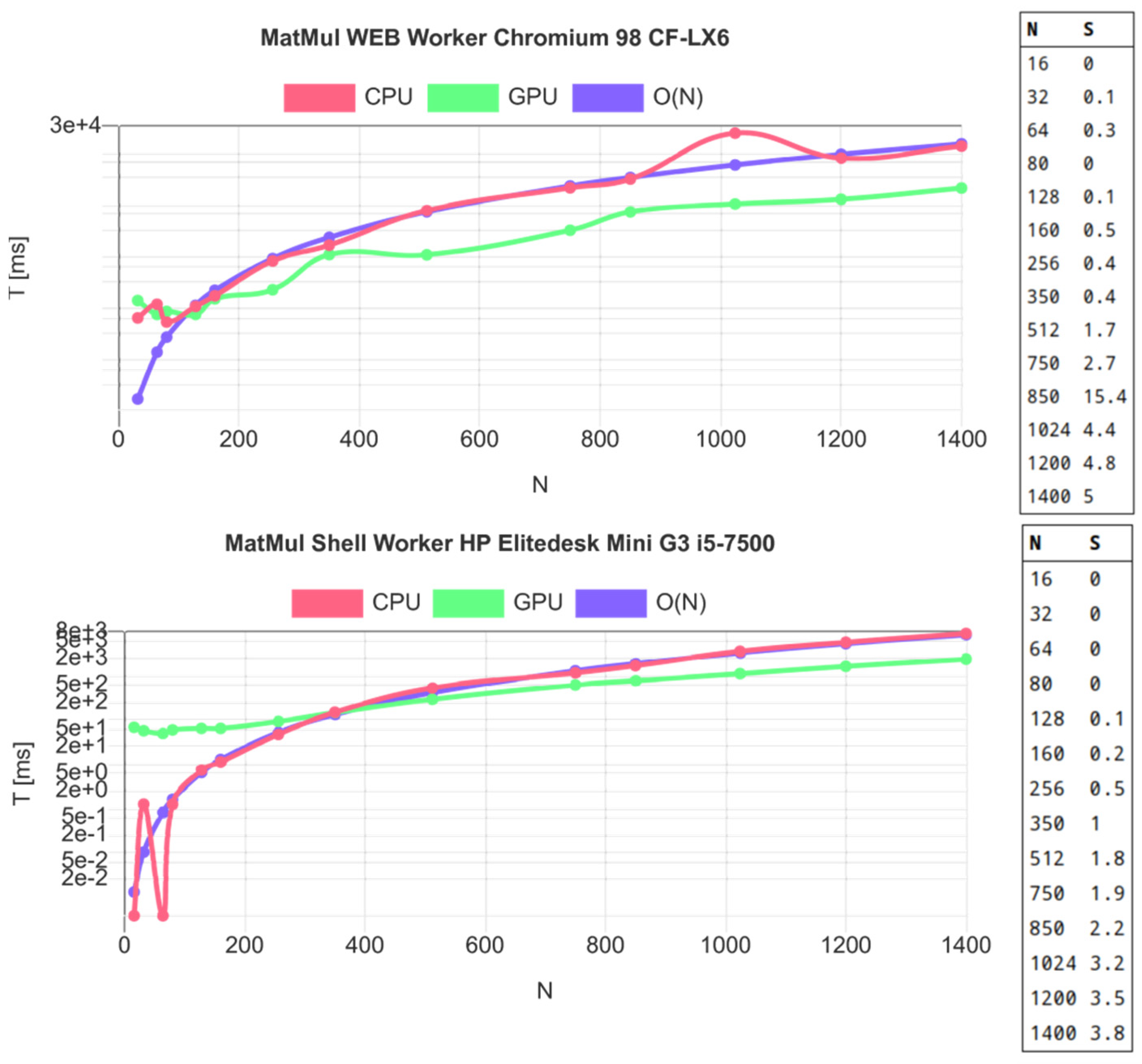
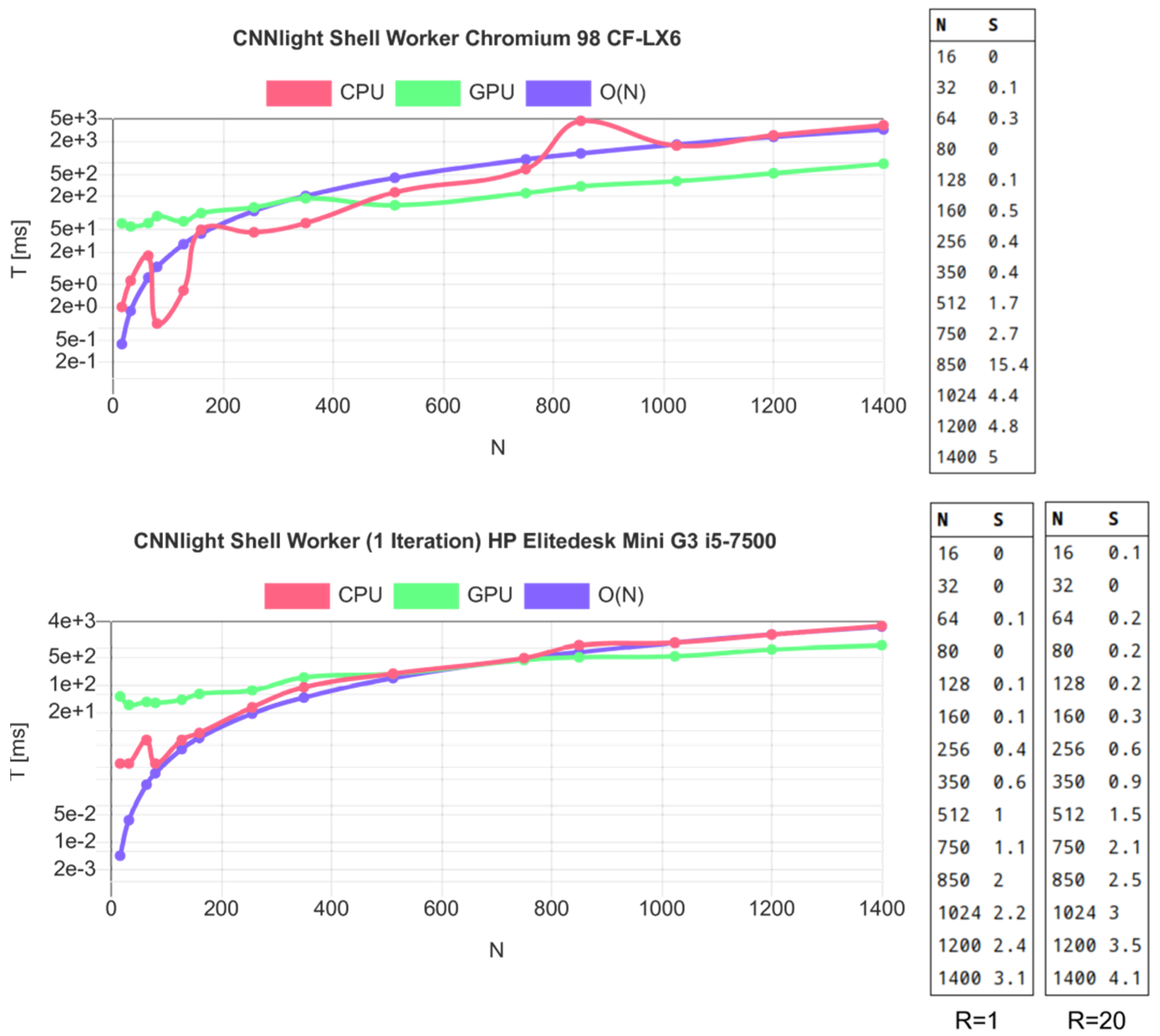
7.2. Evaluation

The following analysis shows some selected experiments for a single-matrix multiplication and a pipelined computation that is typical for an ML task with CNN models performing matrix convolution (O(N²)) and fully connected perceptron layers, containing summation and a functional application (sigmoid function) to all elements of the input matrix (vector) (up to an O(N³) complexity). The figures show the computation times for CPU and GPU processing, depending on the matrix size N. On the right side, the tables show the achieved CPU/GPU speeding-up.

Using generic integrated GPUs (Intel), a speeding-up of up to 5 could be achieved depending on the data size, CPU, JS VM, and GPU, as shown in Figure 7 and Figure 8. The matrix data were stored in flat and compact binary Float32 arrays. The top figure analysis shows the results achieved in a WorkBook worker, and the bottom figure analysis shows the results achieved with WorkShell workers. Below a threshold of about N = 300, the speeding-up is below 1 when using GPU processing. The reasons are the CPU-GPU memory transfer and GPU warm-up times becoming dominant for small-loop iterations.

The processing time of Vanilla JS follows the expected O(N³) complexity, except in the web browser, where is a strong degradation around N = 1000 that was also observed in different browsers. The reason is unknown, but it is expected that L3 data cache flooding by increased matrix data size is invalidated by the decreasing execution time beyond N > 1000. It may be that the memory garbage collection of the VM (Google V8) has a relevant impact, although there is no major data allocation during the test (all input, intermediate, and output matrix data were allocated before computation). Up to N = 512, the computational time using the JS VM CPU is only about two times slower than an optimized native code (C) implementation.

The pipelined CNN light computation shows similar results for both web and shell workers (host platforms with integrated Intel GPU) with a typical speeding-up of about 3–4. For CPU computations this is irrelevant; the GPU computation shows a slight speeding-up if the computation is performed repeatedly (R > 1) in a loop, without any intermediate CPU-GPU memory transfers (bottom figure, second-right table), which is typical for ML training processes.

This analysis shows clearly that the deployment of GPGPU for medium data-path parallelism is only of benefit for large matrix sizes and matrix loop iterations. In particular, the V8 engine already poses a high nearly native code performance for compact and nested loop iterations over matrix data. This observation is in accordance with the analysis performed in [16].

8. Case Studies

8.1. Test Framework

The evaluation of the PSciLab software framework, with its unified processing and communication architecture, in terms of speeding up and scaling up by parallel processing, is performed using different hardware and software platforms, as summarized in

Table 3. Test hardware and software platforms (¹ node.js, ² Firefox 52, ³ Chrome 89, ⁴ Chrome 90, ⁵ high-performance cores, ⁶: low-performance cores, T_st: start-up time/worker, WS: WorkShell and shell worker, WB: WorkBook and web worker, WW: Web WorkShell and web worker).

Acronym	Class	NC	Jystones	Tst	TDP	Eff. η
HPG3	WS	4	9800 k	200 ms	65 W	600
HPZ620	WS	2 × 6	7100 k	490 ms	105/210 W	405
XEON	WS	4	11,200 k	300 ms	84 W	533
RP3B	WS	4	745 k	5000 ms	5 W	596
CFLX3	WB	2	6700 k 1 2700 k 2	150 ms	15 W	890 1 360 2
CFLX6	WB	2	8200 k 1 10,400 k 4	80 ms	25 W	656 1 832 2
G3	WW	2	140 k 3	-	5 W	56
G7	WW	4	340 k 3	-	7 W	388
XL	WW	4 + 4	360 k 3,5/280 k 3,6	-	5 W	576

. Both shell and web worker classes are addressed. To compare the different hardware architectures and systems with each other, a dhrystone benchmark is performed. The dhrystone benchmark combines different typical high-level operations: object allocation and release, function calls, array and string operations, and numerics. The original dhrystone was adapted to JavaScript (from an already existing dhrystone adaptation for Python). The (js)dhrystone results are important key measures for the pool server to estimate the computational power of a host and to balance worker distribution. Another important key measure is the starting-up time of a new worker. Finally, computational efficiency is computed for each example of computer architecture:

$$\eta =\frac{kjsdhrystones\cdot \mathrm{NC}}{\mathrm{TDP}}\left[\frac{1}{Ws}\right]$$

(3)

The thermal dissipation power (TDP) is related to the CPU power consumption and offers another key measure to assess the computer system power for numerical computations. NC is the number of processor cores.

• HPG3-WS: HP G3 Mini, Intel i5-7500 CPU @ 3.40 GHz, 8 GB DRAM, 6 MB L3 Cache, 4 Cores, Debian 10, WorkShell, node.js v8
• HPZ620-WS: HP Z620 Workstation, Intel Xeon CPU E5-2667 0 @ 2.9 GHz, 2 CPU, 6 Cores/CPU, Debian 10, WorkShell, node.js v8 |
• XEON-WS: Intel Xeon Server, Intel Xeon CPU E3-1225 v3 @ 3.2 GHz, 4 Cores, 8 MB L3 cache, 16 GB DRAM, Debian 10, WorkShell, node.js v8 |
• RP3B-WS: Raspberry 3B, ARMv7 Processor rev 4, BCM 2837, 4 Cores @ 1.2 GHz, 1 GB DRAM, 512 kB L2 cache, Debian 10, WorkShell, node.js v10 |
• CFLX3-WB: Panasonic Notebook CF-LX3, Intel i5-4310U @ 3.0 GHz, 8 GB DRAM, 3 MB L3 cache, 2 Cores, SunOS 11.3, WorkBook, Firefox 52
• CFLX6-WB: Panasonic Notebook CF-LX6, Intel i5-7300U @ 3.5 GHz, 8 GB DRAM, 3 MB L3 cache, 2 Cores, Debian 10, WorkBook, Chromium 90
• G3-WB: Motorola Moto G3 smartphone, Qualcomm Snapdragon 410 8916 CPU @ 1.40 GHz, 4 Cores, 1 GB DRAM, Android OS 5.1, WorkBook, Chromium 89
• G7-WB: Motorola Moto G7 smartphone, Qualcomm Snapdragon 632 CPU @ 1.8 GHz, 8 Cores, 2 GB DRAM, Android OS 10, WorkBook, Chromium 89
• XL-WB: Unihertz Atom XL smartphone, Helio P60 CPU @ 2.0 GHz, 4 HP and 4 LP Cores, 2 MB L3 Cache, 6 GB DRAM Android OS 10, WorkBook, Chromium 89

The following two case studies will be used to investigate the capability of parallel and distributed data processing by evaluating the speeding-up S and the parallel scaling index σ:

$$\begin{array}{l}S=\frac{T_1}{T_{PN}}\\ \sigma =\frac{S}{PN}\end{array}$$

(4)

where T is the computation time, with a specific parameter set, and PN is the number of parallel worker processes. The comparison of different computers for a specific computational task, requiring T₁ (in seconds) for single-process execution, can be expressed by the R factor:

$$R=kjsdhrystones\cdot \frac{T_1}{1000}$$

(5)

For a dynamic-sized (or dynamically growing) problem, where the number of processes PN = DN grows linearly with the number of independent computed data (or model) sets DN, there is:

$$\begin{array}{l}S=\left(DN\right)\cdot \frac{T_1}{T_{PN}}\\ \sigma =\frac{S}{PN}\end{array}$$

(6)

The parallelization of a static-sized problem with partitioning aims to reduce the total computation time, whereas a dynamic-sized problem aims to keep a constant total computation time.

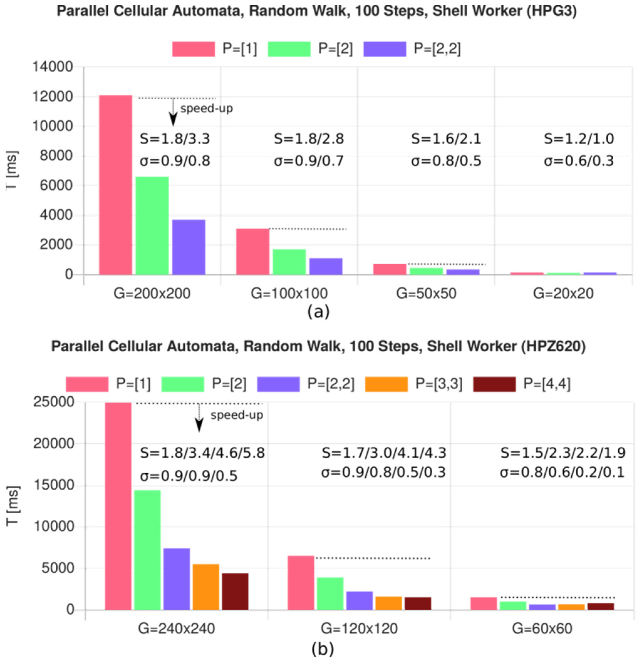
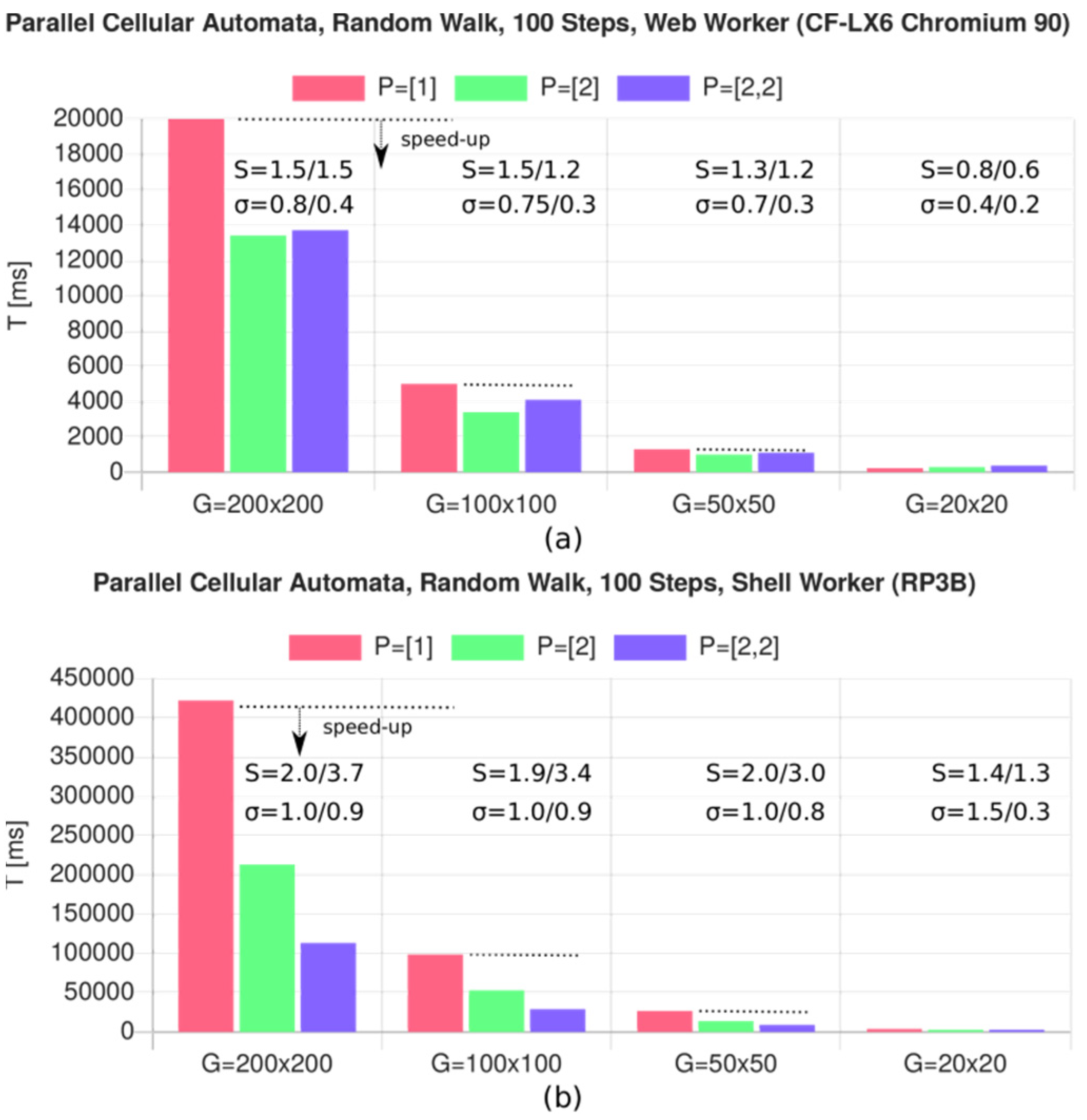
8.2. Simulation with Parallel Cellular Automata

Computation and simulation using cellular automata (CA) are well-suited for distributed and parallel processing, due to the short-range data dependencies. A rectangular and regular cell grid is assumed. The two-dimensional cell grid world can be partitioned in initially independent sub-partitions. Only the partition boundaries require data exchange. Typically, a cell of a CA requires only the state variables from some of the neighboring cells (the Moore and von Neuman neighborhood, with a radius typically within one or two hops). The partitioning of the CA world (cell grid) enables parallel processing. The data state of a cell consists of private variables s and public variables S. The private state must only be shared with the neighboring cells. Only those cells near the partition boundary (with a neighbor partition) require communication by messaging or using shared memory, as shown in Figure 9.

The CA world is partitioned into M partitions. The number of parallel processed partitions depends on the total number of cells N. To benefit from parallel processing, the communication overhead must be considered carefully, which is also dependent on the communication class. Message-based communication is expensive; shared memory communication is more efficient, but it still increases the cell access time to their own state variables.

To minimize communication and memory complexity, private state variables are only shared with other partitions within the neighborhood radius, using slice-shared memory arrays, and public (globally visible) state variables (the output of a cell) are merged in a compact shared memory matrix, limiting the types of these state variables to atomic data types, like integer numbers.

The case study is a simple particle random-walk simulation. The model is shown in Example 11. The full source code can be found in Appendix A. A more complex example using the PSciLab software framework can be found in [28], where longitudinal and spatial infection development is studied. The results from the simple random walk simulation can be directly transferred to the more complex infection simulation. Additionally, the simulation world was partitioned into different spatial domains (e.g., home and working area), enabling more efficient parallel and distributed processing.

var model = {
  rows:20, columns:20, partitions:[2,2],
  parameter : { P:0.3 },
  radius : 1, neighbors : 8,
  cell : {
    private : { id:0, next : null },
    shared : { place : 0 },
    public : { color : 0 },
    before : function (x,y) {
      if (this.place==0) return;
      this.next = this.ask(this.neighbors,‘random’,‘place’,0)
    },
    activity : function (x,y) {
      if (this.place==0) return;
      if (this.next) this.next.place=this.id;
    },
    after : function (x,y) {
      if (this.next && this.next.place == this.id) {
        this.place=0; // we have won the competition
      }
      this.next=null;
      this.color=this.place==0?0:1
    },
    init : function (x,y) {
      this.id=1+this.model.rows*y+x;
      if (Math.random() < this.P) this.place=this.id;
      else this.place=0;
      this.next=null; this.color=this.place==0?0:1
    }
  }
}
var simu = CAP.Lib.SimuPar(model,{print:Code.print});
await simu.createWorker()
await simu.init()
await simu.run(100)
		

• Example 11. CA random-walk model, used for the parallel simulator (here, with 2 × 2 partitions).

The simulator processes the cells in three phases that are synchronized by three barriers: Before, Activity, After. This three-phase protocol is required to avoid race conditions, due to the concurrent modification of shared memory objects. In the first phase, each cell with place ≠ 0 selects one neighbor cell randomly with place = 0 (not occupied). In the main activity, each occupied cell allocates the next place with their unique identifier number. In the third phase, the current place occupation is only removed if the occupant ID won a possible neighbor-cell competition (i.e., next.place is equal to the current identifier number), otherwise, the current occupant stays in the original cell. The problem size is constant; the partitioning of the CA world in smaller parallel-processed sub-partitions should create a speeding-up of the overall simulation time (per simulation step).

Experimental results are shown in Figure 10 for desktop and workstation computers and in Figure 11 for web browsers. The scaling for parallel computing is under-linear and the speeding-up saturates, mostly due to the bottleneck of the shared memory architecture of the host platform. Even on a 2 CPu/12-core workstation, the maximal speeding-up is below 6 (12 is expected). The embedded low-resource Raspberry 3 computer scales up to PN nearly linearly equal the number of cores (4) and sufficient large-grid worlds. The speeding- and scaling up generally decreases with decreasing grid size (and the number of cells per partition).

The product of the simulation times (one process) and measured (j) dhrystone benchmark values (relative CPU scaling) R = k jystones·T₁(s)/1000 for a grid size of 200 × 200 cells is not constant over the different host architectures using the V8 JS core engine (Bytecode + just-in-time native code compilation), showing limited suitability for host selection and computational time predictions (e.g., by the pool server):

• CFLX6 (Chromium 90): R = 208
• HPG3 (node.js): R = 117
• HPZ620 (node.js): R = 177
• RP3B (node.js) R = 305

The memory architecture (shared memory bus and cache memory architecture, number of RAM access ports) of the used host platform seems to have a significant impact on the performance and computational times. The next case study does not use shared memory, showing closer R values.

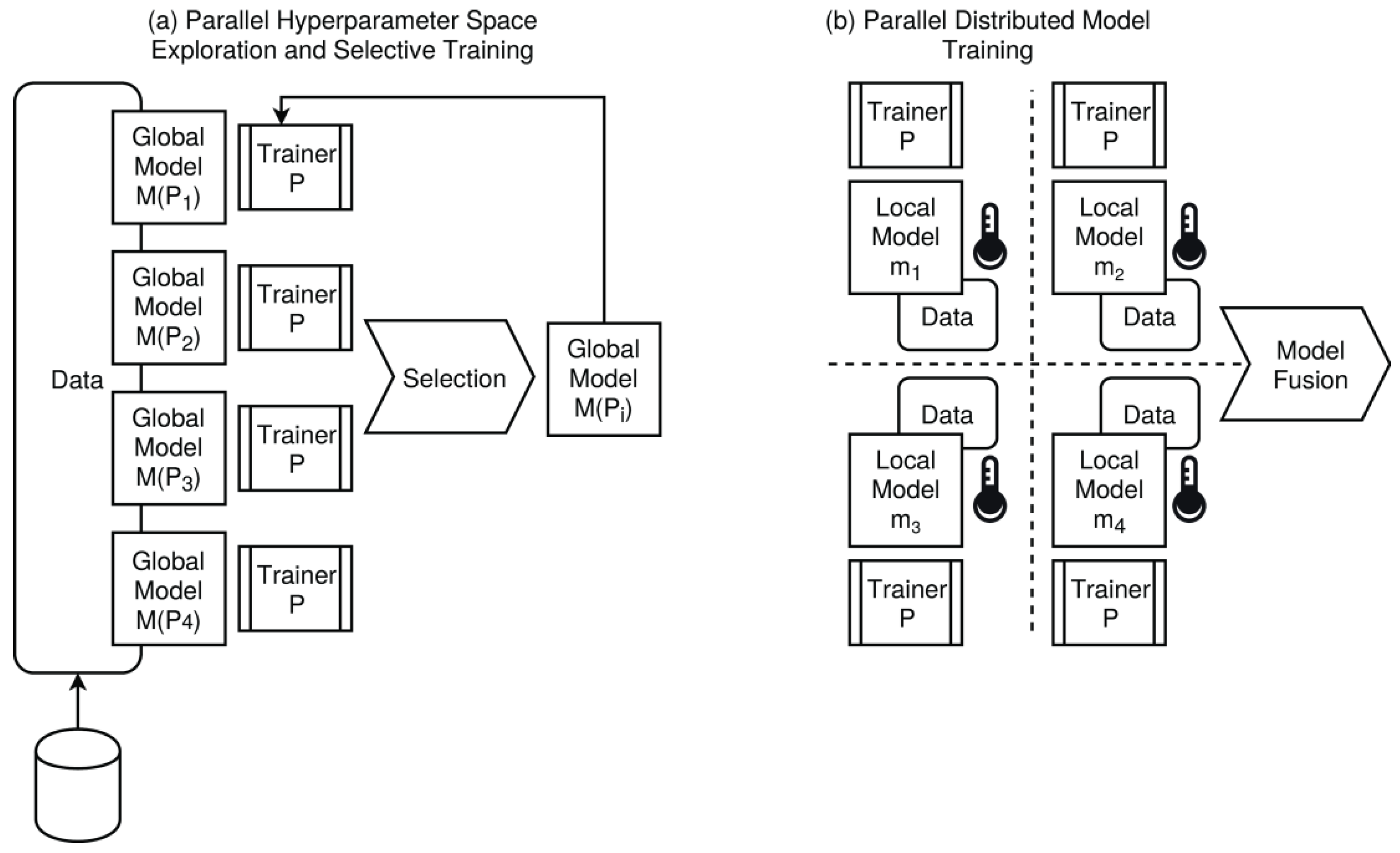
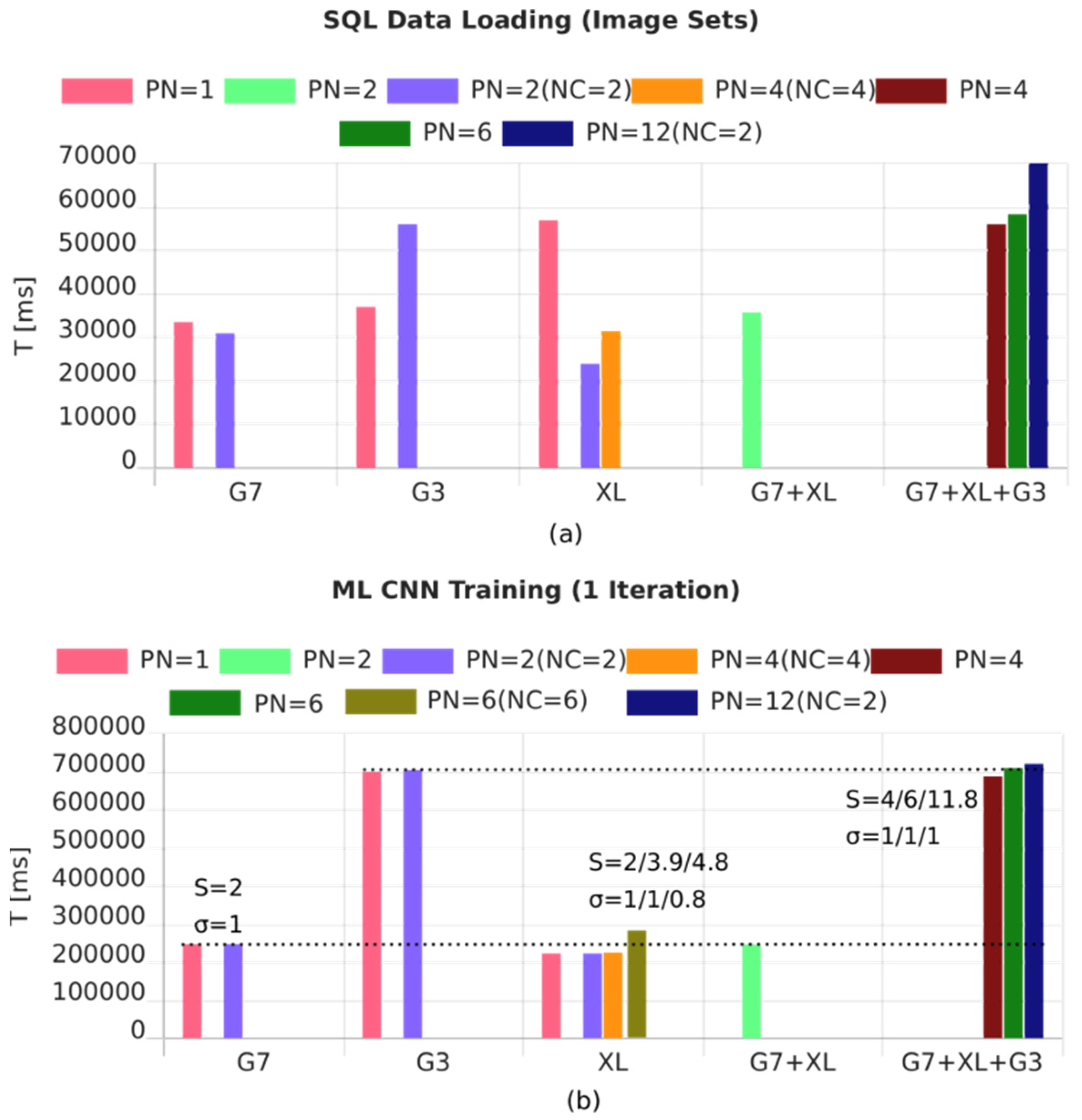
8.3. Multi-Model and Distributed-Parallel Ensemble Machine Learning

ML model training from data is an iterative parameter optimization problem, based on a set of data samples and an error (loss) function. It is difficult to parallelize the training of a single model on a control-path level using workers. Therefore, in this case study, parallel multi-model training is demonstrated and evaluated. It is assumed that there is a set of independent models, either inherently, by a distributed data problem, or by creating a forest of models for best-of selection, or by applying model fusion methodologies (like random forest trees), as shown in Figure 12.

Different models with different parameter settings (and/or structural complexity) can be investigated in parallel. In heterogeneous clusters, the processing nodes can vary in computational power and memory capacity. The relative computational power, measured in dhrystones, can be used to map the computational tasks on nodes. For example, there may be models with different numbers of parameters (neural nodes) and model structures. Smaller models can be processed by slower nodes, and larger models by faster nodes, while still preserving a constant-time scaling (dynamic size problem).

All shell workers have direct access to the extended Math and ML modules. The web worker must load the extended Mathematics and ML plug-ins first. It is assumed that the master process can create the requested worker instances on a remote WorkShell directly (or within the same web browser instance, using web workers).

for(var i=0;i<P;i++) workers[i]=
  new Worker(‘ws:shellhost..’,i);  Shell worker remotely
  new Worker(‘ws:proxyhost..’,i);  or Pool Proxy
  new Worker(i); // or Web/Shell worker locally 
 
for(var i=0;i<P;i++) await workers[i].ready();
function loadAndProcessData(OPTIONS) {
  var db = DB.sql(OPTIONS)
  for (i=1;i<ROWS;i++)
    data.push(await db.select(INPUTDATATABLE,‘*’,‘rowid=’+i);
  var data = data.map(function (row) { return SQL2DATA(row) }
      data = data.map(function (row) { return ML.scale(row,scale) }
  var parts = ML.split(data,TRAINPART,TESTPART)
  this.dataTrain = parts[0]; this.dataTest = parts[1];
  send({ RESULT })
}
function createModel(OPTIONS) {
  this.model = ML.learner(ML.ML.ANN, { OPTIONS })
  send({ RESULT })
}
function trainModel(OPTIONS) {
  ML.train(this.model,this.dataTrain, { OPTIONS })
  send({ RESULT })
}
function testModel(OPTIONS) {
  ML.predict(this.model,this.dataTest, { OPTIONS })
  send({ RESULT })
}
// Four sequential phases 
 
for(var i=0;i<P;i++)
  workers[i].evalf(loadAndProcessData,OPTIONS); // async call 
   
for(var i=0;i<P;i++)
  results[i]=await workers[i].receive(), checkResult(results[i])
for(var i=0;i<P;i++) workers[i].evalf(createModel,OPTIONS); // async call 
 
for(var i=0;i<P;i++)
  results[i]=await workers[i].receive(), checkResult(results[i])
for(var i=0;i<P;i++)
  workers[i].evalf(trainModel,OPTIONS); // async call 
   
for(var i=0;i<P;i++)
  results[i]=await workers[i].receive(), checkResult(results[i])
for(var i=0;i<P;i++)
  workers[i].evalf(testModel,OPTIONS);  // async call 
   
for(var i=0;i<P;i++)
  results[i]=await workers[i].receive(), checkResult(results[i])
		

• Example 12. A typical ML multi-model training program, with hybrid parallel-distributed worker clusters (shortened form).

The problem size in this case study is dynamically growing. Each new worker trains a new independent model, i.e., the number of workers PN is equal to the parallel training of PN models from the same input training data. For the sake of comparability, it is assumed that models trained in parallel differ only in their parameter state (i.e., due to randomness in the training process) but they are structurally equal, with the same computational complexity. The training is incremental and selective. Due to the stochastic initialization of the model parameters and, optionally, stochastic gradient descent (SGD) training (selecting single data instances randomly), the different models develop differently and demonstrate different training progress, as given by the loss function. During parallel training, the best models are selected for further training iterations. Additionally, different model network configurations (static model parameters) can be evaluated, i.e., performing a parallel hyperparameter space exploration.

The problem used is a typical image classification problem (here, with 4 different class labels). A standard convolutional neuronal network (CNN) was used. The input data consist of a large set of small-segment images (64 × 64 pixels) taken from 4 K underwater images; the output is the prediction of a scene class from a set of classes (three different scene classes). The CNN software framework that was used was derived from the ConvNet.js framework [29]. The CNN model had the following configuration and the trainer was an adadelta algorithm:

layers:[
  {type:‘input’, out_sx:64, out_sy:64, out_depth:3},
  {type:‘conv’, sx:5, filters:8, stride:1, pad:2, activation:‘relu’},
  {type:‘pool’, sx:2, stride:2},
  {type:‘conv’, sx:5, filters:16, stride:1, pad:2, activation:‘relu’},
  {type:‘pool’, sx:3, stride:3},
  {type:‘softmax’, num_classes:4}
]
trainer : {method: ‘adadelta’,
  l2_decay: 0.002,
  batch_size: 10}
		

Different worker cluster architectures were investigated, as shown in Figure 13. The entire image data set consists of about 1900 64 × 64 × 3 RGB image volumes (8 bits/element). The training and test data were split 1:1, randomly, i.e., about 900 training and 900 test images. The loading from local and remote SQL data bases, the pre-processing times, and the ML-CNN training times for one epoch (iteration) using shell workers are shown in Figure 14.

The entire ML task is divided into four phases (the first three are considered in this experiment):

• Loading of the input data.
• Pre-processing of the input data (creation of training and test data, data normalization, filtering).
• Model training (here, a CNN), generally the major contribution to the overall computation time.
• Test and verification.

Each shell worker process allocated about 400 MB of working memory for executing all phases. The entire image data set and CNN input data required 1900 × 64 × 64 × 3 × 4 (float32) = 84 MB. Therefore, it is recommended to use 64-bit versions of node.js to access more than 2 GB of memory and computers with at least 2–4 GB of memory/core.

The best single-instance training performance was achieved on the embedded HPG3 platform (4 cores) with a 44 ms/iteration/image data volume. The 2 CPU 6-Core HP Z620 workstation shows higher computational times for single-instance training by about 25%. This experiment, with the same ANN architecture and input data, was conducted with the native code Tensorflow 2.0 framework, using the CPU back-end (and an HP Z620 comparable host platform). The single-instance training time was about 20 ms/iteration/image data volume set in this setup. The JS VM processing can compete with this, even if processed in web browsers, shown in Figure 15. The experiments considered parallel processing on one physical node utilising multi-core CPU processing. Up to the number of cores Web browsers show appropriate scaling efficiency about 0.7. A distributed-parallel worker-tree with different physical nodes would also scale linearly, except for the data transfer via LAN.

Maximal speeding-up S = PN is achieved in this dynamically growing size problem if the overall computation time keeps constant with an increasing PN, under the assumption that all processes have the same workload (computation time). The scaling up (speeding-up with respect to the number of parallel worker processes, PN) is nearly linear, up to the maximal number of CPU cores, i.e., S ≈ NC. The total loading time of the input data (1800 images) does not increase significantly up to PN = NC and is independent of the SQL server location (local or remote). The remote SQL data base access only increases the loading time by a factor of two (when using 1 Gb/s LAN; the data consumer and source nodes were connected by the same LAN switch). Note that about 10–30 CNN training iterations (epochs) were required to achieve a good prediction accuracy of about 80–90%.

Processing on the Raspberry PI3B platform only allowed one training process, due to memory constraints (a worker requires about 300–400 MB of memory). The loading time of the input data from a remote SQL data base (using 1 Gb/s LAN; the data consumer and source nodes were connected by the same LAN switch) required about 8.0 s, the pre-processing of the input data, about 8.3 s, and the training, about 670 s. This slow down relates approximately to the measured (j)dhrystone value ratio of 1:11. It is well known that node.js underperforms on ARM platforms (the V8 core engine was designed and optimized for x86/x64 platforms).

The product of the ML training times (for a single process) and the measured (j)dhrystone benchmark values (relative CPU scaling) R = k jystones·T₁(s)/1000 is nearly constant over the different host architectures, regardless of whether the V8 JS core engines (Bytecode + just-in-time native code compilation) or pure Bytecode engines (Firefox) are used, showing the suitability for host selection and computational time predictions (e.g., by the pool server) for ML tasks:

• CFLX3 (Firefox 52): R = 472
• CFLX6 (Chromium 90): R = 540
• HPG3 (node.js): R = 381
• HPZ620 (node.js): R = 372
• RP3B (node.js): R = 498

In contrast to parallel simulations relying on shared memory processing, the scaling and performance of parallel ML tasks depend mostly on the CPU, not on the memory architecture. The V8-based web browsers (with native-code JIT support, e.g., Chrome) pose similar computation times compared with workstations and desktop computers, and a speeding-up of about 2–3 times compared with pure Bytecode engines (like Spidermonkey, as used in Firefox). Even the older browsers are suitable for ML computations (no significant speeding-up could be observed for Firefox 73 over 52).

Two more experiments were carried out, which demonstrates the universal distributed computing capabilities of the PSciLab software framework.

The next experiment performed hybrid distributed-parallel processing with four computer nodes (3 × 4 cores, 3 × HPG3, and 2 × 6 CPU cores, 1 × HPZ620), a total of 24 CPU cores. The results are shown in Figure 16. There is a nearly constant scaling σ = 1. Note that the last first five experiments were carried out with only 3 × HP-G3 computers, the last two with an additional HP-Z620 workstation that poses a lower dhrystone ranking (about 30% lower), which decreases the accumulated speeding- and scaling up. Adjusting this ratio, the corrected scaling-up is still equal to 1 up to 24 parallel workers.

The last experiment exploits computational power on ubiquitous devices like smartphones. Using the web WorkShell, one task-specific script file, the proxy server, and a WorkBook session, it is possible to create a large-scale distributed computer. The proxy/group service, as part of the pool server, provided a WebSocket virtual circuit service, simple group management, and an HTTP file server. All smartphones are connected via one WLAN access point (Huawei WS5200). The web WorkShell is loaded by the smartphones via the proxy server, finally loading the script file from the proxy server as well. The script connects to the proxy server and adds a unique peer identifier to a task-specific group. Finally, the script provides an RPC service loop, waiting for remote script processing (similar to the RPC service provided by web and shell workers). The WorkBook master program, processed in a web browser, distributes functional tasks to the remote smartphone workers. Results for the same multi-model CNN-ML training task using 6 smartphones are shown in Figure 17. Note that the computational and communication power differ among the devices (see Table 3) and there can be a mix of high- and low-performance cores. There is a nearly linear scaling up of the speeding-up with the number of processes PN. Although, unexpectedly, the speeding-up scales up nearly linearly with the number of cores in the smartphones. The overall performance of smartphones for numerical tasks is low compared with servers, but distributed-parallel computation can compensate sufficiently for this. The R-value for new-generation smartphones (Moto G7, Atom XL) performing ML-CNN training is lower (about 70) than on Intel x86-based systems (about 300), i.e., the ML code is executed more efficiently. The total average data loading time via the remote SQL service increases under-linearly and is comparable to Web browser environments on desktop computers. The data loading time is still negligible compared with the ML training times. Typically, 10–20 epochs are required to derive a suitable model.

In [30], the ML problem consisted of independent multi-instance learning and multi-instance inference, with independent and partitioned input data, i.e., basically a distributed and localized multi-model ML system (finally deployed in a distributed sensor network) with global model fusion. The PSciLab framework was used to train all models in parallel. Again, a linear scaling-up to the number of cores NC was observed (an HPZ620 platform was also used). In this case study, the problem size was static and was fixed with a similar partition schema, as used in the parallel simulation.

To summarize, multi-model ML training scales up nearly linearly with the number of worker processes, up to the number of CPU cores. Hyper-threading provides no additional improvement when using VM processing. Both web browser and node.js-based processing using the V8 core VM of ML tasks perform equally. In contrast to shared-memory-based simulation, parallel ML tasks do not rely significantly on the memory architecture of the host platform. The data exchange times (input, intermediate, output) using SQLite data bases are negligible compared with the training times of medium and large-size models (typically, a ratio of 1:100). Even one SQLite service scales up well under parallel data stream processing; multi-data-base services can improve scaling.

9. Conclusions

The introduced software framework and the processing and communication architecture are suitable for implementing common computationally intensive numerical tasks, like simulation and ML, using web browsers and/or node.js as execution platforms. A hierarchical and hybrid distributed-parallel worker process composition is supported, providing parallelism on a control-path level, with an API not requiring expert knowledge of the programming of parallel and distributed systems. Worker processes can be easily created with only a few lines of code. Functional or procedural code can be executed on a worker (regardless of whether it is a local or a remote worker) by synchronous or asynchronous single operations. Data and functional code can be serialized and sent to a worker. Static and dynamic size problems are addressed, and two case studies demonstrate suitable scaling up with an increasing number of worker processes. Control-path parallelism can be supplemented with data-path parallelism using GPU, via the WebGL/OpenGL API. Parallelism can be exploited by replacing numerical vanilla JS code with respective kernel-based GPU code, using a GPGPU plug-in, but extensive analysis showed only a medium degree of speeding up for large-scale data problems.

It can be seen that a JavaScript version of the dhrystone benchmark is suitable for estimating the computational power of computing nodes for typical numerical problems like ML with message-based communication but is not accurate for problems with a shared memory architecture (like simulations). The dhrystone measures can be used by the pool server to select the appropriate computing nodes. The pool server includes a virtual circuit proxy and group service. Multiple distributed pool servers can be connected.

The central element for large-scale distributed numerical systems is data storage management. Data are stored and exchanged by worker processes using a customized SQLite data base. An RPC layer was added to enable remote data base access, using a JSON-SQL query format. Multiple distributed data bases can be used to distribute data base workload. Data tables can be copied between SQL data bases in advance (progressive data management). The failure of worker processes can be handled by restarting workers from a check-point state that contains the relevant data. Actually, it is up to the programmer to handle worker failures by performing manual check-pointing via the SQL data bases. Automatic check-pointing with snapshots that are optimally supported directly by the pool server needs to be implemented to provide reliable distributed computing.

The entire framework and all user code are programmed using the widely established programming language JavaScript, executed on virtual machines, most notably Google’s V8 and Mozilla’s Spidermonkey engines. Two extended case studies, with additional references to additional scientific published work using this framework, show the suitability, efficiency, and mostly linear scaling of the multi-process architecture using worker processes. Worker processes can be spawned locally or remotely, using either web or shell workers. Code can be interchanged between both worker classes seamlessly. There is communication between the master (main) and worker processes, established via message channels, either using internal UNIX sockets or pipes (with worker processes established from the same master process) or WebSockets (worker processes can be established remotely). Besides message-based communication, shared memory approaches and the SBO architecture enable the sharing between workers of composed objects like data records, mono-typed arrays, and matrix objects, using linear buffers by providing direct high-level programming access, as for any other JS object. Additionally, IPC objects, like barriers, are implemented via the shared memory. The high performance of message-based and shared memory communication could thus be shown.

The evaluation of the case studies shows the high efficiency of hybrid distributed-parallel processing using widely available hardware, including smartphones. Distributed processing scales up nearly linearly, i.e., S ≈ PN. The set of worker processes contains local and remote-controlled processes, as well as web and shell workers, which can be mixed arbitrarily, and the processes can be executed efficiently in parallel on multi-core computers.

In this work, smartphones using common web browsers enable participative crowd computing using the web WorkShell. However, this approach requires explicit user activity and, if the web page is closed, the worker processes are also lost. The next step is the transition from participative to opportunistic (hidden) crowd computing, using service workers processing modified headless web WorkShell software. Service workers are persistent and are processed beyond the lifetime of a web page (typically up to 30 s), including re-incarnation. Check-pointing via the browser cache is required to survive re-incarnation and to provide scheduled long-term computation.

References

1. PsiLAB 1/2. Scientific and Numeric Research Software Environment. Available online: http://psilab.sourceforge.net (accessed on 1 January 2022).
2. node.js. Available online: https://github.com/nodejs/node (accessed on 1 January 2022).
3. Choy, R.; Edelman, A. Parallel MATLAB: Doing It Right. Proc. IEEE 2008, 93, 331–341. [Google Scholar] [CrossRef] [Green Version]
4. Liu, X.; Ounifi, H.A.; Gherbi, A.; Li, W.; Cheriet, M. A hybrid GPU-FPGA based design methodology for enhancing machine learning applications performance. J. Ambient. Intell. Humaniz. Comput. 2020, 11, 2309–2323. [Google Scholar] [CrossRef]
5. Romano, J. WebMesh: A Browser-Based Computational Framework for Serverless Applications. Bachelor’s Thesis, Computer Science Department, Brown University, Providence, RI, USA, 2019. [Google Scholar]
6. Nicol, D.; Fujimoto, R. Parallel simulation today. Ann. Oper. Res. 1994, 53, 249–285. [Google Scholar] [CrossRef] [Green Version]
7. Magee, J.; Dulay, N.; Kramer, J. Structuring parallel and distributed programs. Softw. Eng. J. 1993, 8, 73. [Google Scholar] [CrossRef]
8. Bagrodia, R.; Meyer, R.; Takai, M.; Chen, Y.A.; Zeng, X.; Martin, J.; Song, H.Y. Parsec: A parallel simulation environment for complex systems. Computer 1998, 31, 77–85. [Google Scholar] [CrossRef] [Green Version]
9. Kao, A.; Krastins, I.; Alexandrakis, M.; Shevchenko, N.; Eckert, S.; Pericleous, K. A parallel cellular automata lattice Boltzmann method for convection-driven solidification. Jom 2019, 71, 48–58. [Google Scholar] [CrossRef] [PubMed] [Green Version]
10. Rosin, P.L. Training Cellular Automata for Image Processing. IEEE Trans. Image Process. 2002, 15, 2076–2087. [Google Scholar] [CrossRef] [PubMed]
11. Giordano, A.; De Rango, A.; Rongo, R.; D’Ambrosio, D.; Spataro, W. Dynamic load balancing in parallel execution of cellular automata. IEEE Trans. Parallel Distrib. Syst. 2020, 32, 470–484. [Google Scholar] [CrossRef]
12. Xia, C.; Wang, H.; Zhang, A.; Zhang, W. A high-performance cellular automata model for urban simulation based on vectorization and parallel computing technology. Int. J. Geogr. Inf. Sci. 2018, 32, 399–424. [Google Scholar] [CrossRef]
13. Aaby, B.G.; Perumalla, K.S.; Seal, S.K. Efficient Simulation of Agent-Based Models on Multi-GPU and Multi-Core Clusters. In Proceedings of the 3rd International Icst Conference on Simulation Tools and Techniques, Malaga, Spain, 15–19 March 2010. [Google Scholar]
14. Xiao, J.; Andelfinger, P.; Eckhoff, D.; Cai, W.; Knoll, A. A Survey on Agent-based Simulation using Hardware Accelerators. ACM Comput. Surv. 2019, 51, 1–35. [Google Scholar] [CrossRef]
15. Hughes, D.; Correll, N. Distributed Machine Learning in Materials that Couple Sensing, Actuation, Computation and Communication. arXiv 2016, arXiv:1606.03508. [Google Scholar]
16. Ma, Y.; Xiang, D.; Zheng, S.; Tian, D.; Liu, X. Moving Deep Learning into Web Browser: How Far Can We Go? In Proceedings of the World Wide Web Conference, San Francisco, CA, USA, 13–17 May 2019. [Google Scholar]
17. Teerapittayanon, S.; McDanel, B.; Kung, H.T. Distributed deep neural networks over the cloud, the edge and end devices. In Proceedings of the 2017 IEEE 37th International Conference on Distributed Computing Systems (ICDCS), Atlanta, GA, USA, 5–8 June 2017; IEEE: Piscataway, NJ, USA, 2017; pp. 328–339. [Google Scholar]
18. Chahal, K.S.; Grover, M.S.; Dey, K.; Shah, R.R. A hitchhiker’s guide on distributed training of deep neural networks. J. Parallel Distrib. Comput. 2020, 137, 65–76. [Google Scholar] [CrossRef] [Green Version]
19. Schlegel, D. Deep Machine Learning on GPUs; University of Heidelber-Ziti: Mannheim, Germany, 2015. [Google Scholar]
20. NVIDIA. cuDNN Developer Guide; PG-06702-001_v8.3.2; Available online: https://docs.nvidia.com/deeplearning/cudnn/developer-guide/index.html (accessed on 1 February 2022).
21. Kotsifakou, M.; Srivastava, P.; Sinclair, M.D.; Komuravelli, R.; Adve, V.; Adve, S. Hpvm: Heterogeneous parallel virtual machine. In Proceedings of the 23rd ACM SIGPLAN Symposium on Principles and Practice of Parallel Programming, Vienna, Austria, 24–28 February 2018; pp. 68–80. [Google Scholar]
22. Graham, R.L.; Shipman, G.M.; Barrett, B.W.; Castain, R.H.; Bosilca, G.; Lumsdaine, A. Open MPI: A high-performance, heterogeneous MPI. In Proceedings of the 2006 IEEE International Conference on Cluster Computing, Barcelona, Spain, 25–28 September 2016; IEEE: Piscataway, NJ, USA, 2017; pp. 1–9. [Google Scholar]
23. Han, J.; Haihong, E.; Le, G.; Du, J. Survey on NoSQL database. In Proceedings of the 2011 6th International Conference on Pervasive Computing and Applications, Port Elizabeth, South Africa, 26–28 October 2011; IEEE: Piscataway, NJ, USA, 2017; pp. 363–366. [Google Scholar]
24. Peteiro-Barral, D.; Guijarro-Berdinas, B. A Survey of methods for distributed machine learning. Prog. Artif. Intell. 2013, 2, 1–11. [Google Scholar] [CrossRef] [Green Version]
25. Sarafov, V. Comparison of IoT Data Protocol Overhead. In Proceedings of the Seminars FI/IITM WS 17/18, Network Architectures and Services, Munich, Germany, 1 August 2017–26 February 2018; pp. 7–14. [Google Scholar]
26. PSciLab Software Repository. Available online: https://github.com/bsLab/PSciLab (accessed on 21 February 2022).
27. gpu.js. Available online: https://github.com/gpujs/gpu.js (accessed on 1 January 2022).
28. Bosse, S. Parallel and Distributed Agent-based Simulation of large-scale socio-technical Systems with loosely coupled Virtual Machines. In Proceedings of the SIMULTECH Conference 2021, International Conference on Simulation and Modeling Methodologies, Technologies and Applications, Online, 7–9 July 2021. [Google Scholar]
29. ConvNet.js, Deep Learning in the Browser. Available online: https://cs.stanford.edu/people/karpathy/convnetjs/ (accessed on 1 December 2021).
30. Bosse, S.; Weiss, D.; Schmidt, D. Supervised Distributed Multi-Instance and Unsupervised Single-Instance Autoencoder Machine Learning for Damage Diagnostics with High-Dimensional Data—A Hybrid Approach and Comparison Study. Computers 2021, 10, 34. [Google Scholar] [CrossRef]
Figure 1. PSciLab software framework and its components (right) and WorkBook GUI layout (left) using code snippets flows with micro consoles.
Applsci 12 02887 g001
Figure 2. The cluster approach: heterogeneous processing architecture with web browsers (WorkBook) and node.js (WorkShell), connected via the intra- and internet. Parallel execution is provided by spawned WebWorker and ShellWorker.
Applsci 12 02887 g002
Figure 3. Different communication methods are used to connect the cluster nodes and their worker processes. The Web Service port is used for remote worker control.
Applsci 12 02887 g003
Figure 4. Process pipelines, composed of code snippet processes pi, interconnected by channel queues. Additionally, code snippet processes can exchange data via shared-state variables.
Applsci 12 02887 g004
Figure 5. The pool manager server (PMS), managing and connecting worker process groups.
Applsci 12 02887 g005
Figure 6. Shared buffer objects: architecture and programmatical access.
Applsci 12 02887 g006
Figure 7. (Top) WorkBook worker/WebGL; (bottom) WorkShell worker/OpenGL: performance analysis of an N × N matrix multiplication, using Vanilla JS and GPU transpiled kernel functions (Integrated Intel GPU).
Applsci 12 02887 g007
Figure 8. (Top) WorkBook worker/WebGL; (bottom) WorkShell worker/OpenGL: performance analysis of a data flow pipeline with 1 matrix kernel convolution, a fully connected perceptron layer merging the convoluted matrix with the application of a sigmoid function, and a second, fully connected perceptron layer (R: number of loop iterations).
Applsci 12 02887 g008
Figure 9. The basic partitioned architecture of the CA. Each partition of the CA world is executed in a separate process. Data exchange is performed via shared memory.
Applsci 12 02887 g009
Figure 10. Parallel simulation results using shell worker processes, showing the total simulation time for 100 simulation steps in dependency of the parallel partitions (rows, cols), S: speeding up, σ: scaling up, (a) HP-G3 mini (b) HP-Z620 workstation.
Applsci 12 02887 g010
Figure 11. (a) Parallel simulation results using Web worker processes showing total simulation time for 100 simulation steps (b) Results for shell worker processes executed on an embedded computer (Raspberry PI 3+); S: speeding up, σ: scaling up.
Applsci 12 02887 g011
Figure 12. Parallel multi-model training: (a) model diversity; (b) distributed models using local sensor data.
Applsci 12 02887 g012
Figure 13. The distributed-parallel worker architectures used for multi-model ML training: (a) parallel web workers managed by a WorkBook; (b) distributed-parallel shell workers; (c) distributed web WorkShell workers; WB: WorkBook, WS: WorkShell, WWS: Web WorkShell.
Applsci 12 02887 g013
Figure 14. Results of the total computation times, with shell worker processing of multi-model CNN-ML tasks with a different number of workers (PN). S: speeding up, σ: scaling up, HPG3: NC = 4, HPZ620: NC = 12. (a) Input data loading times from the SQL data base; (b) data pre-processing times; (c) training times.
Applsci 12 02887 g014
Figure 15. Results of the total computation times, with web worker processing of multi-model CNN-ML tasks with a different number of workers PN. CF-LX3/LX6: NC = 2. (a) Input data loading times from SQL data base; (b) data pre-processing times; (c) training times.
Applsci 12 02887 g015
Figure 16. Results of the total computation times, with a distributed-parallel cluster, with shell workers processing multi-model CNN-ML training using a different number of distributed and parallel workers PN. HPG3: NC = 4, HPZ620: NC = 12.
Applsci 12 02887 g016
Figure 17. Results of the total computation times, with a distributed-parallel cluster with web workers, processed on smartphones and performing multi-model CNN-ML training with different numbers of distributed and parallel workers: (a) SQL data loading times; (b) ML training times (1 iteration = 1 epoch).
Applsci 12 02887 g017