
Variable Rate Independently Recurrent Neural Network (IndRNN) for Action Recognition


1
School of Software, Shandong University, Jinan 250101, China
2
Weihai Research Institute of Industrial Technology, Shandong University, Weihai 264209, China
3
State Key Laboratory of Dynamic Testing Technology and School of Information and Communication Engineering, North University of China, Taiyuan 030051, China
4
School of Control Science and Engineering, Shandong University, Jinan 250100, China
5
School of Computer Science and Engineering, University of Electronic Science and Technology of China, Chengdu 611731, China
*
Author to whom correspondence should be addressed.
Appl. Sci. 2022, 12(7), 3281; https://0-doi-org.brum.beds.ac.uk/10.3390/app12073281
Submission received: 21 January 2022
/
Revised: 17 March 2022
/
Accepted: 22 March 2022
/
Published: 23 March 2022
(This article belongs to the Special Issue Computer Vision and Pattern Recognition Based on Deep Learning)
Abstract
:Recurrent neural networks (RNNs) have been widely used to solve sequence problems due to their capability of modeling temporal dependency. Despite the rich varieties of RNN models proposed in the literature, the problem of different sampling rates or performing speeds in sequence tasks has not been explicitly considered in the network and the corresponding training and testing processes. This paper addresses the problem of different sampling rates or performing speeds in the skeleton-based action recognition with RNNs. Specifically, the recently proposed independently recurrent neural network (IndRNN) is used as the RNN network due to its well-behaved and easily regulated gradient backpropagation through time. Samples are extracted with variable sampling rates and thus of different lengths, then processed by IndRNN with different time steps. In order to accommodate the differences in terms of gradients introduced by the backpropagation through time under variable time steps, a learning rate adjustment method is further proposed in the paper. Different learning rate adjustment factors are obtained for different layers by analyzing the gradient behavior under IndRNN. Experiments on skeleton-based action recognition are conducted to verify its effectiveness, and the results show that the proposed variable rate IndRNN network can significantly improve the performance over the RNN models under the conventional training strategies.
1. Introduction
Recurrent neural networks have been widely used for sequence problems, such as action recognition, speech recognition and language modeling [1,2,3,4,5]. For different tasks, different sampling strategies may be used. Even for one task, the sampling strategy, such as the sampling rate, may be different due to the different sensors used for capturing data. In spite of a rich varieties of the RNN models, the training strategies are usually the same and not adaptively adjusted to different situations. Taking skeleton-based action recognition [6,7], for example, a common strategy is to divide an instance into equal-length segments, and one frame is drawn from each segment to compose the final input. In this way, samples of the same length are drawn from sequences and used as input. Models trained with such inputs may not generalize well in practice when the sensors used to capture data are changed with a different sampling rate. On the other hand, the performing speeds of different samples may also be different. However, the number of actors performed in each dataset is usually limited (for example, 40 for the NTU RGB+D dataset containing 56,880 sequences [6]), and they are usually in a rather similar range of age, rendering similar action speeds of the whole dataset. By contrast, in real-world applications, the speeds of one action performed by different people are usually different. Consequently, the models trained with inputs of fixed speed may not generalize well. With samples obtained with different or non-uniform sampling rates and performing speeds between the training data and test data (in practice), the underlying semantic meaning of the observation at a time step is misaligned and, thus, the network cannot perform well.
Another problem in training RNNs is the learning with sequences of varying lengths. When one sequence is extracted with different sampling rates, the lengths of the extracted samples are correspondingly different. Therefore, the RNN network needs to process sequences of varying lengths. With the recurrent connections of RNNs, RNNs can be naturally extended to process sequences of different lengths. However, the time steps gradient backpropagated is different when the lengths of the sequences are different. Accordingly, to make RNNs work with sequences of different lengths, the learning rate needs to be adjusted to adapt to the gradient changes. In spite of that, in most of the training strategies, the learning rate is set to be the same for different lengths. There are only few works [8,9] on using RNNs with different lengths in the literature, which linearly adjusts the learning rate based on the length of the sequence (the longer, the larger). In contrast, in this paper, based on the recently proposed IndRNN [10,11,12], the learning rate adjustment can be obtained analytically and we demonstrate that the opposite works (the longer, the smaller), although it is not simply the inverse of a linear function.
The contributions of this paper can be summarized as follows.
- A variable rate IndRNN model is proposed to solve the problem of varying sampling rates or performing speeds that may exist between different sequences or between training and test (in practice). The model processes inputs of different lengths and extracted with different sampling rates.
- An adaptive learning rate adjustment method is proposed based on the lengths of the sequences that the IndRNN network processes. Different adjustment factors are obtained for different layers with different gradient propagation properties.
Experiments were conducted on the skeleton-based action recognition task. Results show that the proposed variable rate IndRNN model achieves better performance than the conventional fixed-rate model and achieves state-of-the-art performance using RNNs.
The rest of the paper is organized as follows. Section 2 describes the related work in the area of skeleton-based action recognition with RNNs, and Section 3 explains the basic backgrounds on the recently proposed IndRNN, including its structure and gradient backpropagation process. The proposed method is presented in Section 4, and the experiments are shown in Section 5. Finally, the conclusion is drawn at Section 6.
2. Related Work
With the increasing popularity of depth sensors, such as Kinect, skeleton-based action recognition [6,7,13,14] has drawn lots of interest over the last few years. Many conventional methods with handcrafted features have been proposed, such as the HON4D [15], using histograms of the surface normal orientation in the 4D space of time, depth, and spatial coordinates to obtain features. Similarly, the dynamic skeletons method [16] uses a modified HOG (histogram of oriented gradients) method to dynamically collect features at each frame and then extract features again with HOG. With the rapid development of deep learning, deep learning models, including the convolutional neural networks (CNNs) [17,18,19,20,21,22,23], graph convolution neural networks (GCNs) [24,25,26] and the recurrent neural networks (RNNs) [6,7,13,14,27,28,29,30,31], have been widely studied for skeleton-based action recognition methods. Among them, CNN- and GCN-based methods mostly focus on the extraction of spatial features, especially the GCN-based ones. For example, in AGNN [24], the skeletons are treated as an undirected graph, and graph convolution is used to extract spatial features in a way of spectral graph filtering. For the temporal processing, RNNs are also used to gather the temporal information. Considering that this paper mainly addresses the temporal processing for action recognition, in the following, only some typical RNN-based methods are reviewed.
Most of the existing RNN-based methods investigate the grouping property of skeleton joints, where the joints move together in a group. Such a property was explored in [6,13,32] with hierarchical RNNs, joint co-occurrence RNNs, or part-aware RNNs. In these methods, several joints (such as joints on the left hand) are usually considered as a part by adding extra layers or constraints to group the joints, and then the models process the parts instead of the joints. There are also methods [14] using geometric features of the skeleton joints to explore the geometric relationships between different joints. Another type of method employs the attention models [29,30] to exploit the property that joints may not show equal importance in classifying different actions. The attention weights on the joints at different time steps are different to focus on different joints for different actions. Another method worth mentioning is the recently proposed independent recurrent neural network (IndRNN), which effectively solves the gradient vanishing and exploding problem and can be used to construct deep models and process long sequences. It reported the best results so far achieved by the RNN-based methods on the NTU RGB+D dataset (the largest dataset with skeleton for action recognition) [6]. While the above methods investigate specific features and models for skeleton-based action recognition, none of them explicitly consider the effect of different performing speeds and different sampling rates of the actions. The current prevailing ad hoc approach to dealing with this is to sample sequences of a fixed length by separating the action sequence into fixed-length segments and extracting one frame from each segment. In this way, for each sequence, the sampling rates are the same at different extractions, although variations may exist for each frame. The proposed method deals with both variable performing speeds and variable sampling rates (due to the PC used for capturing and the RGB-D sensors for instance).
Furthermore, while RNNs are widely used in action recognition, the training strategies are usually the same, with one learning rate for all equal-length inputs, and there is not much research on training RNNs with inputs of variable lengths. In [9], an unbiased truncated gradient backpropagation through time (BPTT) was proposed, where the learning rate is adjusted based on the probability of the sequence with different lengths in order to compensate for the difference between truncated backpropagation through time (BPTT) and the un-truncated one. However, the learning rate for the original (un-truncated) BPTT is still empirically set, and the learning rate is increased with the increase in the input length. This strategy was also adopted in [8], where the learning rate is linearly increased with the increase in the input length. By contrast, in this paper, based on the recently proposed IndRNN, we show that the opposite works, where the learning rate drops with the increase in the input length.
3. Overview of IndRNN
Independently recurrent neural network (IndRNN) was proposed in [10] as a basic RNN component. It follows
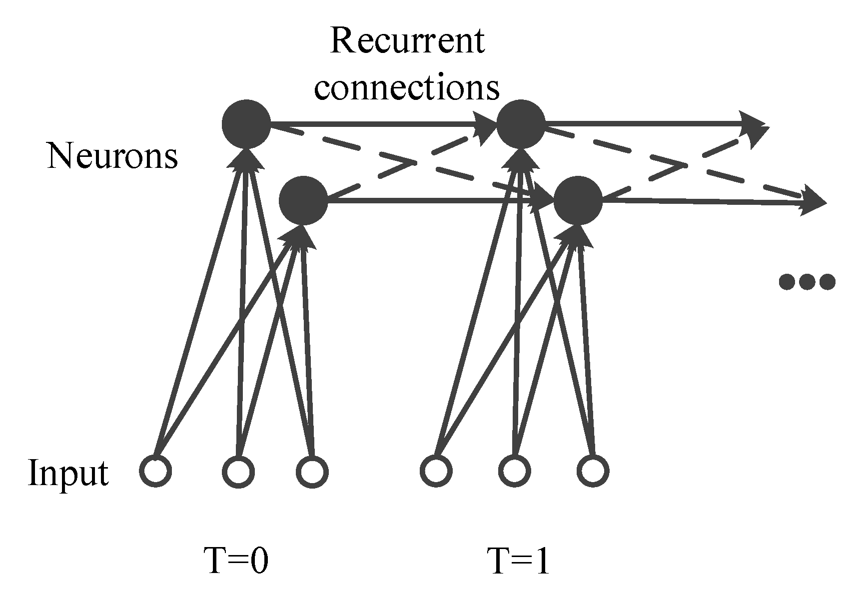
where and are the input and hidden state at time step t, respectively. , and are the weights for the current input, the recurrent input, and the bias of the neurons. ⊙ represents the Hadamard product (element-wise multiplication). is an element-wise activation function of the neurons, which is the ReLU (rectified linear unit) in this paper, and N is the number of neurons in this IndRNN layer. Each neuron in one layer is independent from others as shown in Figure 1 and the correlation among neurons is explored by stacking two or more layers of IndRNNs. IndRNN solves the gradient vanishing and exploding problems, and can be used to process long sequences and construct deeper networks. Better results than the existing RNN networks on various tasks, including skeleton-based action recognition, were reported in [10].
Since neurons in one IndRNN layer are independent from each other, the gradient backpropagation through time can be calculated for each neuron individually. For the n-th neuron , where the bias is ignored, suppose the objective trying to minimize at time step T is . Then the gradient backpropagated to the time step t is
where is the derivative of the element-wise activation function. For more details on the above derivation, please refer to [10,11].
4. Proposed Variable Rate IndRNN
In this section, we first present the variable rate sampling strategy and the corresponding network architecture, then deduce the learning rate adjustment method for different layers in the network architecture.
4.1. Variable Rate Sampling Strategy and Network Architecture
To make the network more robust to various sampling rates and performing speeds of different sequences, inputs of different sampling rates and performing speeds need to be provided for training. With respect to the performing speeds (per frame) of the captured data, it can be changed in the same way by changing the sampling rates used to generate the input to the network. Therefore, in the proposed method, variable sampling rates are used to provide inputs of both different sampling rates and performing speeds to the network. In the following, the variable rate sampling strategy based on the equal-length sampling used in the skeleton-based action recognition task is explained, and it can be easily extended to other tasks.
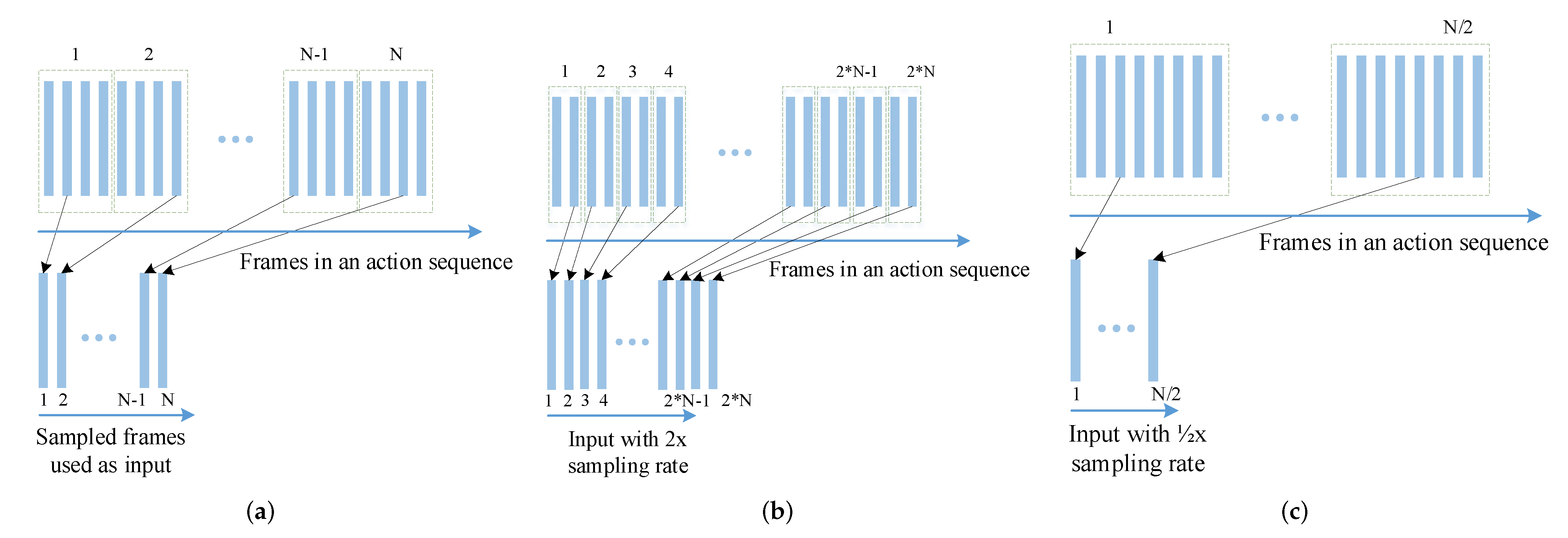
For one skeleton sequence, the inputs extracted with different sampling rates would be of different lengths. Figure 2 illustrates the sampling strategy with different sampling rates. First, the conventional sampling method is shown in Figure 2a, where N is the length of the sampled input. Assume there are L frames in the sequence, then the sampling rate is L/N. In the training process, the sequence is separated into N segments, and each frame is sampled from one segment to compose the final input. Although for different inputs, frames sampled from one segment may be different, the overall sampling rate and speed are the same. The proposed variable rate sampling strategy uses different sampling rates to generate inputs of different rates and speeds. Figure 2b,c illustrates two examples with higher (2×) and lower (1/2×) sampling rates, respectively. It is obvious that with higher sampling rates, more frames are contained in the input, and vice versa.
In the proposed method, IndRNN is used as the classification network. The architecture of the IndRNN network with variable sampling rates is shown in Figure 3. It is composed of several (denoted by L) IndRNN layers (with batch normalization layers inserted after each IndRNN layer). A fully connected (FC) layer with the softmax function is used for the output. With the inputs of variable lengths, the RNN network also processes dynamic time steps. As shown in Figure 3, when the sequence is longer, IndRNN will keep processing more inputs, and the fully connected layer will be added at the end of the time steps for classification. The same applies to shorter sequences, where fewer time steps are processed. Since the network processes inputs of different lengths, the statistics of the batch normalization layers at each time step are kept individual, while the weight parameters are shared over time.
4.2. Learning Rate Adjustment
As shown in Figure 3, the gradient behaviors for the final FC layer, the last IndRNN layer and the other IndRNN layers are different. For the final FC layer, the gradient is directly backpropagated from the objective and no backpropagation through time is required. For the last IndRNN layer, the gradient is only backpropagated from the final FC layer, but the gradient is further backpropagated through time. For the other IndRNN layers, the gradient is backpropagated from its previous layers at each time step and further backpropagated through time. In the following, the learning rate adjustment for these three groups are discussed separately.
4.2.1. Learning Rate Adjustment for the First IndRNN Layers
For the first IndRNN layers, the gradient consists of two parts: the gradient backpropagated from the previous layer and the gradient backpropagated from the previous time steps. For IndRNN, the neurons are independent from each other at each layer, and the gradient can be calculated for each neuron independently. For the gradient of the n-th neuron at time step t, it can be obtained according to Equation (2) as
where is the gradient of the current step, and are the gradients of the future time steps.
Since here we mainly focus on the gradient backpropagated through time, the small differences among the gradients backpropagated from the previous layer at different time steps are ignored, and the gradients are all denoted by . In this paper, the ReLU (rectified linear unit) is considered the activation function and its gradient is either 0 or 1 based on whether the neuron is activated. Denoting the probability of a neuron being activated by p, can be statistically simplified to . Thus, the above Equation (3) can be simplified as
The final gradient can be obtained by summarizing the gradients over all the time steps from 1 to T, and can be expressed as
when does not equal 1. When equals 1, . Usually is no larger than 1 when the sequence length is large, and p is smaller than 1. Therefore, is smaller than 1, and the above equation stands.
On the other hand, suppose there is no gradient backpropagation through time; at each time step, the IndRNN network becomes the conventional feedforward network, and the training process becomes training a network with a large mini batch (but the gradient is summarized instead of being averaged over batches, which is ). As shown in [33], when the mini batch size is multiplied by k, the learning rate multiplied by k usually provides good performance by assuming that the gradients of the mini batches equal the gradients at different training iterations. In this case, when no gradient backpropagation through time is considered, the learning rate of the conventional feedforward network can be directly used since the summation (instead of average) of the gradients works as the linear scaling of the learning rate.
To accommodate the gradient differences introduced by the gradient backpropagation through time, the learning rate needs to be adjusted accordingly. The learning rate adjustment factor can be obtained based on their gradients as
where is the learning rate adjustment factor. With , the magnitudes of the changes to the network parameters under gradient backpropagation through time are similar to those of the conventional feedforward network.
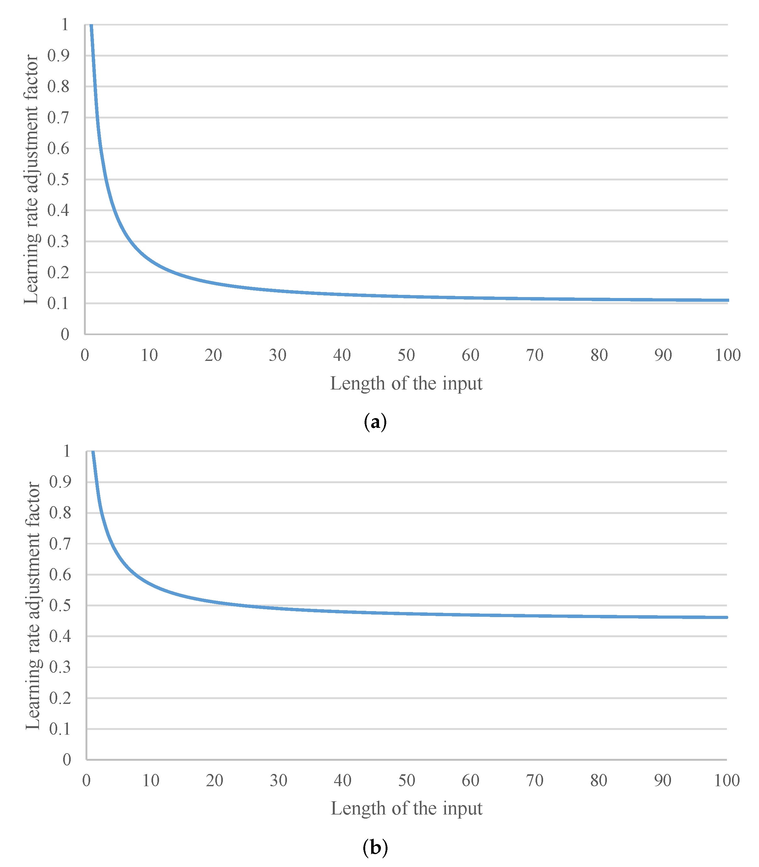
The basic probability of the neurons activated is assumed to be since half of the input range is activated for the ReLU function. With the recurrent connection, the neuron is more likely to be activated, as the recurrent input is usually no smaller than 0 (with positive recurrent weight). The larger the recurrent weight, the higher the probability of the neuron being activated. In the implementation, the probability of the neurons activated is set as , where the highest probability reaches when equal 1. Figure 4a illustrates the learning rate adjustment factors over different lengths of inputs when the recurrent weight is set to 1. It can be seen that the learning rate adjustment factor drops quickly at first, and then decays steadily around when the length of the input is over 30 steps.
To avoid the complex calculation for each recurrent neuron, the average learning rate adjustment factor is used for all the neurons. With the recurrent weight uniformly initialized in the range of , the average learning rate adjustment factor can be obtained as
It can be numerically obtained as shown in Figure 4b, where 1000 recurrent weights with interval 0.001 is used. Similar behavior as above for the recurrent weight 1 can be observed, which is shown in Figure 4b. The learning rate adjustment factor drops quickly at first and decays steadily around when the length of the input is over 30 steps. Note that if two IndRNN layers are directly stacked together, the gradient of the first IndRNN layer , backpropagated from the second IndRNN layer, has already been affected by the gradient backpropagation from the time of the second IndRNN layer. In such a case, is different from the conventional feedforward network. However, in the proposed IndRNN network, batch normalization layer is inserted between IndRNN layers, and the statistics of the input to each layer is changed, which also affects the gradient backpropagation process. Therefore, for simplicity, of all the IndRNN layers is considered the same as the conventional feedforward network, and no further adjustment is used for different layers.
4.2.2. Learning Rate Adjustment for the Last (L-th) IndRNN Layers
For the last (L-th) IndRNN layer, the gradient is only backpropagated from the final FC layer at the last time step and then further backpropagates to other time steps. Therefore, based on Equation (4), by summarizing the gradients backpropagated from the last time step to different time steps, its gradient can be expressed as
when does not equal 1. In the case of equaling 1, it simply follows . Accordingly, the learning rate adjustment factor can be set as , when does not equal 1. When equals 1, the learning rate adjustment factor can be set as , which decreases linearly based on the length of the input. However, as noted before, is usually smaller than 1; therefore, the first equation stands. For the last IndRNN layer, since only the output at the last time step is used, the recurrent weights can be initialized to relatively large values to only keep long-term memory, as in [10]. Here, the recurrent weights are assumed to be in the range . Similar to the learning rate adjustment factor for the first layers shown above, the average learning rate adjustment factor is used and can be numerically obtained as shown in Figure 5 over different lengths of inputs. Similar behavior as that of the first layers can be observed but decays slightly faster than the neurons in the first layers.
4.2.3. Learning Rate Adjustment for the Final FC Layers
For the final FC layer, the gradient backpropagation process is the same as that of conventional feedforward networks since no gradient backpropagation through time is needed. Therefore, the learning rate adjustment factor is set to 1.
5. Experiments
The proposed method is evaluated on two large-scale datasets, including the NTU RGB+D dataset [6] (the largest skeleton based action recognition dataset so far), and the UOW large scale combined (LSC) dataset [34]. Adam optimization [35] is used with the initial learning rate . The learning rate for each layer under the inputs of different lengths is adjusted based on the learning rate adjustment factor as shown in Section 4.2. The overall learning rate is decayed by 10 once the evaluation accuracy does not increase (with patience 100). Dropout is applied after each layer with the same dropping mask shared over time. The detailed dropping probability for each dataset is further described in the following Subsections. The lengths are sampled with a normal distribution . For the NTU RGB+D dataset [6], m is set to 20, which is the most widely used in the existing works. For simplicity, the sequence length used in each batch is set to be the same, and the lengths of different batches are different. The IndRNN network, consisting of 6 layers and 512 neurons, is used as in [10]. The other training setups are similar as in [10]. Following the convention, the testing results are reported in the following experiments. Since this paper focuses on the investigation of the RNN-based skeleton action recognition, the graph convolution based ones [25,26] are not discussed nor compared.
5.1. Results on NTU RGB+D Dataset
The NTU RGB+D dataset [6] contains 56,880 sequences of 60 action classes, collected by three Kinect v2 cameras with 17 different setups. A total of 40 subjects of ages from 10 to 35 years, are involved to performed the action sequences. Two evaluation protocols, including cross-subject (CS) and cross-view (CV) settings, are suggested for evaluation. For the cross-subject setting, the 40 subjects are equally split into training and testing groups. However, the number of samples for different subjects is different, and according to the subject split used in [6], 40,320 and 16,560 samples are used for training and testing, respectively. For the cross-view setting, the samples of camera 1 are used for testing and cameras 2 and 3 are used for training. Each camera is used in several capturing setups (different views), and according to the detailed split used in [6], 37,920 samples and 18,960 samples are used for training and testing, respectively. Additionally, as suggested in [6], 5% of the training data is randomly selected and reserved as evaluation data. Two skeletons (25 joints per skeleton) are used as input; if only one is present in the sample, the second is set as zero. Therefore, the input is of 25 × 2 × 3 = 150 dimensions, containing the 3D coordinates of the skeleton joints. The batch size is set to 128, and the dropping probabilities of and are used for the CS and CV settings, respectively.
5.1.1. Verification of the Effect of Different Sampling Rates
First, to demonstrate the effect of different sampling rates on the testing performance, inputs extracted with different sampling rates are generated and used for training and testing, respectively. The same IndRNN model as in the proposed method is used for training and testing. For training, the same sampling strategy as in [10] is used, where 20 frames are extracted for each sample. For testing, the sampling rate is doubled and, accordingly, 40 frames are extracted from each sequence. The straightforward way of testing is to directly test the sample of 40 frames with the trained network. However, the network is trained with 20 frames, and testing with 40 frames does not work very well. Therefore, 20 frames sampled from the middle half of a sequence to make the frames sampled with a doubled rate is used for testing. The other settings are the same as [10]. The results compared with the training and testing with the same sampling rate are shown in Table 1. It can be seen that when the sampling rates of training and testing are different, the performance drops significantly. The variable rate IndRNN is also tested under different sampling rates, and the results are also shown in Table 1. It can be seen that the variable rate IndRNN works fine for all test rates. The small differences between the baseline IndRNN and the variable rate IndRNN is due to the different training and testing settings for which, for variable rate IndRNN, the lengths of the training sequences are not exactly the same as those of the test sequences. Therefore, it is necessary to train with different sampling rates in order to make the trained model more robust for different data.
5.1.2. Evaluation of the Proposed Method
Table 2 shows the results of the proposed method with variable sampling rates and learning rate adjustment factors in comparison with the existing methods. It can be seen that the proposed method achieves better performance than the existing methods as well as the IndRNN [10]. Additionally, variable sampling rates are also used for the test sequences and the probability of several predictions are averaged to obtain the final result, showing better performance than the variable rate IndRNN with fixed test sampling rates as shown in Table 1. Moreover, it can be seen that the improvement for the CS setting (2.52%) is larger than the CV setting (1.74%). For the CS (cross subject) setting, the performing speeds of different subjects are different, and thus the training and testing may deviate from each other in terms of performing speeds. With the proposed variable rate IndRNN, the deviation can be mitigated and thus the performance is improved significantly as shown in Table 2. On the other hand, for the CV (cross view) setting, the subjects for the training and testing are the same, and thus the effect of various performing speeds is smaller. Therefore, the improvement of the proposed method is smaller than that of the CS setting, although it still improves the performance. Note that the dataset is collected with cameras of the same type, thus the sampling rates are the same. When the dataset is further extended with multiple data sources, the performance may be further improved with various sampling rates.
5.2. Results on UOW Large Scale Combined (LSC) Dataset
The UOW LSC dataset [34] is a large dataset composed of nine publicly available datasets including MSR Action3D Ext [39], UTKinect [40], MSR DailyActivity [41], MSR ActionPair [15], CAD120 [42], CAD60 [43], G3D [44], RGBD-HuDa [45], and UTD-MHAD [46]. There are 94 actions in total. However, samples in some action classes do not contain skeleton modality and thus are excluded in the experiment, resulting in 88 action classes and 3897 samples. The protocols developed in [34] are used for evaluation, including a random cross subject (similar as in the NTU RGB+D setting) and random cross sample. For the random cross sample setting, in each action category, half of the samples are randomly selected for training. The average recall and precision of all classes, as suggested in [34], is used for comparison. The batch size is set to 64, and the dropping probability is set to 0.35 for both protocols. The other settings are the same as those used for the above NTU RGB+D dataset. Table 3 shows the result of the proposed model compared with the existing methods (results obtained from their original papers). It can be seen that better performance can be achieved with the proposed method against the RNN-based ones. For the cross sample setting, it also achieves similar performance as the graph-convolution-based AGNN [24], but worse in the cross subject setting. It is known that graph convolution can obtain better spatial features than simply providing joint coordinates to the RNNs. Therefore, better spatial feature extraction methods are desired for the proposed method and other RNN-based methods.
6. Conclusions
This paper presented a variable rate IndRNN. It solves the problem of varying sample rates and performing speeds by generating inputs with different sampling rates. Accordingly, the IndRNN network processes inputs of different lengths through different time steps. By processing inputs of variable lengths and sampling rates, the network learns to be more adaptive and robust to samples captured with different setups and actions performed with different speeds. Moreover, with the IndRNN dynamically processing inputs of different lengths, the gradient behavior over different inputs is also changed, and the learning rate needs to be adjusted accordingly. By investigating the gradient backpropagation process under IndRNN, a new learning rate adjustment method was proposed, which adaptively accommodates the gradient differences for different layers. Compared with the existing methods, the proposed method can better handle the actions performed under variable sampling rates and variable speeds. Experiments on two large and widely used skeleton dataset were conducted, and better performance over the existing RNN-based methods wa demonstrated by the proposed method.
The proposed method takes an approach of increasing training with sequences of different sampling rates and the corresponding learning strategy, but it is also worth investigating how to directly revise or formulate an IndRNN model dynamically with different sampling rates, instead of just training. Moreover, the proposed method only focuses on the temporal processing, while for the spatial processing, it takes the original joint coordinates as input. Therefore, to further improve the overall action recognition performance, better spatial processing methods are worth investigating, such as graph-convolution-based ones.
Author Contributions
Conceptualization, Y.G., C.L., S.L., M.Y. and H.Y.; methodology, Y.G., C.L., S.L. and X.C.; software, Y.G. and C.L.; investigation, Y.G., C.L., S.L., X.C., M.Y. and H.Y.; writing, Y.G., C.L. and S.L. All authors have read and agreed to the published version of the manuscript.
Funding
This research was partly funded by National Key R&D Program of China (2018YFE0203900), the National Natural Science Foundation of China (No. 61901083, 62001092 and 62101512), Fundamental Research Program of Shanxi Province (20210302124031), the open project program of state key laboratory of virtual reality technology and systems, Beihang University (VRLAB2021A01) and SDU QILU Young Scholars program.
Institutional Review Board Statement
Not applicable.
Informed Consent Statement
Not applicable.
Data Availability Statement
The data presented in this study are available on request from the corresponding author.
Conflicts of Interest
The authors declare no conflict of interest.
References
- Donahue, J.; Hendricks, L.A.; Guadarrama, S.; Rohrbach, M.; Venugopalan, S.; Saenko, K.; Darrell, T. Long-term recurrent convolutional networks for visual recognition and description. In Proceedings of the IEEE Conference on Computer Vision and Pattern Recognition, Boston, MA, USA, 7–12 June 2015; pp. 2625–2634. [Google Scholar]
- Li, C.; Li, S.; Gao, Y.; Zhang, X.; Li, W. A Two-stream Neural Network for Pose-based Hand Gesture Recognition. IEEE Trans. Cogn. Dev. Syst. 2021, 1–10. [Google Scholar] [CrossRef]
- Yue-Hei Ng, J.; Hausknecht, M.; Vijayanarasimhan, S.; Vinyals, O.; Monga, R.; Toderici, G. Beyond short snippets: Deep networks for video classification. In Proceedings of the IEEE Conference on Computer Vision and Pattern Recognition, Boston, MA, USA, 7–12 June 2015; pp. 4694–4702. [Google Scholar]
- Pigou, L.; van den Oord, A.; Dieleman, S.; Van Herreweghe, M.; Dambre, J. Beyond temporal pooling: Recurrence and temporal convolutions for gesture recognition in video. Int. J. Comput. Vis. 2015, 126, 430–439. [Google Scholar]
- Jain, A.; Zamir, A.R.; Savarese, S.; Saxena, A. Structural-RNN: Deep learning on spatio-temporal graphs. In Proceedings of the IEEE Conference on Computer Vision and Pattern Recognition, Las Vegas, NV, USA, 26 June–1 July 2016; pp. 5308–5317. [Google Scholar]
- Shahroudy, A.; Liu, J.; Ng, T.T.; Wang, G. NTU RGB+ D: A large scale dataset for 3D human activity analysis. In Proceedings of the IEEE Conference on Computer Vision and Pattern Recognition, Las Vegas, NV, USA, 26 June–1 July 2016; pp. 1010–1019. [Google Scholar]
- Liu, J.; Shahroudy, A.; Xu, D.; Wang, G. Spatio-temporal LSTM with trust gates for 3D human action recognition. In European Conference on Computer Vision; Springer: Cham, Switzerland, 2016; pp. 816–833. [Google Scholar]
- Merity, S.; Keskar, N.S.; Socher, R. Regularizing and Optimizing LSTM Language Models. arXiv 2017, arXiv:1708.02182. [Google Scholar]
- Tallec, C.; Ollivier, Y. Unbiasing Truncated Backpropagation Through Time. arXiv 2017, arXiv:1705.08209. [Google Scholar]
- Li, S.; Li, W.; Cook, C.; Zhu, C.; Gao, Y. Independently recurrent neural network (indrnn): Building A longer and deeper RNN. In Proceedings of the IEEE Conference on Computer Vision and Pattern Recognition, Salt Lake City, UT, USA, 18–22 June 2018; pp. 5457–5466. [Google Scholar]
- Li, S.; Li, W.; Cook, C.; Gao, Y. Deep Independently Recurrent Neural Network (IndRNN). arXiv 2019, arXiv:1910.06251. [Google Scholar]
- Zhao, B.; Li, S.; Gao, Y.; Li, C.; Li, W. A Framework of Combining Short-Term Spatial/Frequency Feature Extraction and Long-Term IndRNN for Activity Recognition. Sensors 2020, 20, 6984. [Google Scholar]
- Du, Y.; Wang, W.; Wang, L. Hierarchical recurrent neural network for skeleton based action recognition. In Proceedings of the IEEE Conference on Computer Vision and Pattern Recognition, Boston, MA, USA, 7–12 June 2015; pp. 1110–1118. [Google Scholar]
- Zhang, S.; Liu, X.; Xiao, J. On geometric features for skeleton-based action recognition using multilayer LSTM networks. In Proceedings of the 2017 IEEE Winter Conference on Applications of Computer Vision (WACV), Santa Rosa, CA, USA, 24–31 March 2017; pp. 148–157. [Google Scholar]
- Oreifej, O.; Liu, Z. Hon4d: Histogram of oriented 4d normals for activity recognition from depth sequences. In Proceedings of the IEEE Conference on Computer Vision and Pattern Recognition, Portland, OR, USA, 23–28 June 2013; pp. 716–723. [Google Scholar]
- Ohn-Bar, E.; Trivedi, M. Joint angles similarities and HOG2 for action recognition. In Proceedings of the IEEE Conference on Computer Vision and Pattern Recognition, Portland, OR, USA, 23–28 June 2013; pp. 465–470. [Google Scholar]
- Wang, P.; Li, Z.; Hou, Y.; Li, W. Action recognition based on joint trajectory maps using convolutional neural networks. In Proceedings of the 2016 ACM on Multimedia Conference, Amsterdam, The Netherlands, 15–19 October 2016; ACM: New York, NY, USA, 2016; pp. 102–106. [Google Scholar]
- Ke, Q.; An, S.; Bennamoun, M.; Sohel, F.; Boussaid, F. SkeletonNet: Mining Deep Part Features for 3-D Action Recognition. IEEE Signal Process. Lett. 2017, 24, 731–735. [Google Scholar]
- Kim, T.S.; Reiter, A. Interpretable 3D Human Action Analysis with Temporal Convolutional Networks. arXiv 2017, arXiv:1704.04516. [Google Scholar]
- Yue, J.; Gao, Y.; Li, S.; Hui, Y.; Frederic, D. Global Appearance and Local Coding Distortion based Fusion Framework for CNN based Filtering in Video Coding. IEEE Trans. Broadcast. 2022, 1–13. [Google Scholar] [CrossRef]
- Ke, Q.; Bennamoun, M.; An, S.; Sohel, F.; Boussaid, F. A New Representation of Skeleton Sequences for 3D Action Recognition. arXiv 2017, arXiv:1703.03492. [Google Scholar]
- Li, C.; Hou, Y.; Wang, P.; Li, W. Joint Distance Maps Based Action Recognition With Convolutional Neural Networks. IEEE Signal Process. Lett. 2017, 24, 624–628. [Google Scholar]
- Cao, C.; Zhang, Y.; Zhang, C.; Lu, H. Body Joint Guided 3-D Deep Convolutional Descriptors for Action Recognition. IEEE Trans. Cybern. 2018, 48, 1095–1108. [Google Scholar]
- Li, C.; Cui, Z.; Zheng, W.; Xu, C.; Ji, R.; Yang, J. Action-Attending Graphic Neural Network. IEEE Trans. Image Process. 2018, 27, 3657–3670. [Google Scholar]
- Liu, Z.; Zhang, H.; Chen, Z.; Wang, Z.; Ouyang, W. Disentangling and Unifying Graph Convolutions for Skeleton-Based Action Recognition. In Proceedings of the IEEE/CVF Conference on Computer Vision and Pattern Recognition (CVPR), Seattle, WA, USA, 13–19 June 2020; pp. 140–149. [Google Scholar]
- Chen, Y.; Zhang, Z.; Yuan, C.; Li, B.; Deng, Y.; Hu, W. Channel-wise Topology Refinement Graph Convolution for Skeleton-Based Action Recognition. arXiv 2021, arXiv:2107.12213. [Google Scholar]
- Veeriah, V.; Zhuang, N.; Qi, G.J. Differential recurrent neural networks for action recognition. In Proceedings of the IEEE International Conference on Computer Vision, Santiago, Chile, 7–13 December 2015; pp. 4041–4049. [Google Scholar]
- Zhang, C.; Li, S.; Ye, M.; Zhu, C.; Li, X. Learning Various Length Dependence by Dual Recurrent Neural Networks. Neurocomputing 2021, 466, 1–15. [Google Scholar]
- Liu, J.; Wang, G.; Hu, P.; Duan, L.Y.; Kot, A.C. Global context-aware attention lstm networks for 3d action recognition. In Proceedings of the IEEE Conference on Computer Vision and Pattern Recognition, Honolulu, HI, USA, 21–26 July 2017; pp. 1647–1656. [Google Scholar]
- Song, S.; Lan, C.; Xing, J.; Zeng, W.; Liu, J. An End-to-End Spatio-Temporal Attention Model for Human Action Recognition from Skeleton Data. In Proceedings of the AAAI Conference on Artificial Intelligence 2017, San Francisco, CA, USA, 4–9 February 2017; pp. 4263–4270. [Google Scholar]
- Gao, Y.; Li, C.; Li, S.; Cai, X.; Ye, M.; Yuan, H. A Deep Attention Model for Action Recognition from Skeleton Data. Appl. Sci. 2022, 12, 2006. [Google Scholar] [CrossRef]
- Zhu, W.; Lan, C.; Xing, J.; Zeng, W.; Li, Y.; Shen, L.; Xie, X. Co-Occurrence Feature Learning for Skeleton Based Action Recognition Using Regularized Deep LSTM Networks. In Proceedings of the AAAI Conference on Artificial Intelligence 2016, Phoenix, AZ, USA, 12–17 February 2016; Volume 2, p. 8. [Google Scholar]
- Goyal, P.; Dollár, P.; Girshick, R.; Noordhuis, P.; Wesolowski, L.; Kyrola, A.; Tulloch, A.; Jia, Y.; He, K. Accurate, large minibatch SGD: Training imagenet in 1 hour. arXiv 2017, arXiv:1706.02677. [Google Scholar]
- Zhang, J.; Li, W.; Wang, P.; Ogunbona, P.; Liu, S.; Tang, C. A large scale rgb-d dataset for action recognition. In Proceedings of the International Workshop on Understanding Human Activities through 3D Sensors, Cancun, Mexico, 4 December 2016; Springer: Berlin/Heidelberg, Germany, 2016; pp. 101–114. [Google Scholar]
- Kingma, D.P.; Ba, J. Adam: A method for stochastic optimization. arXiv 2014, arXiv:1412.6980. [Google Scholar]
- Huang, Z.; Wan, C.; Probst, T.; Van Gool, L. Deep learning on lie groups for skeleton-based action recognition. arXiv 2016, arXiv:1612.05877. [Google Scholar]
- Liu, M.; Liu, H.; Chen, C. Enhanced skeleton visualization for view invariant human action recognition. Pattern Recognit. 2017, 68, 346–362. [Google Scholar]
- Baradel, F.; Wolf, C.; Mille, J. Pose-conditioned Spatio-Temporal Attention for Human Action Recognition. arXiv 2017, arXiv:1703.10106. [Google Scholar]
- Li, W.; Zhang, Z.; Liu, Z. Action recognition based on a bag of 3d points. In Proceedings of the 2010 IEEE Computer Society Conference on Computer Vision and Pattern Recognition-Workshops, San Francisco, CA, USA, 13–18 June 2010; pp. 9–14. [Google Scholar]
- Xia, L.; Chen, C.C.; Aggarwal, J.K. View invariant human action recognition using histograms of 3d joints. In Proceedings of the 2012 IEEE Computer Society Conference on Computer Vision and Pattern Recognition Workshops, Providence, RI, USA, 16–21 June 2012; pp. 20–27. [Google Scholar]
- Wang, J.; Liu, Z.; Wu, Y.; Yuan, J. Mining actionlet ensemble for action recognition with depth cameras. In Proceedings of the 2012 IEEE Conference on Computer Vision and Pattern Recognition, Providence, RI, USA, 16–21 June 2012; pp. 1290–1297. [Google Scholar]
- Yang, X.; Tian, Y. Super normal vector for activity recognition using depth sequences. In Proceedings of the IEEE Conference on Computer Vision and Pattern Recognition, Columbus, OH, USA, 23–28 June 2014; pp. 804–811. [Google Scholar]
- Sung, J.; Ponce, C.; Selman, B.; Saxena, A. Human Activity Detection from RGBD Images. Plan Act. Intent Recognit. 2011, 64. [Google Scholar]
- Bloom, V.; Makris, D.; Argyriou, V. G3d: A gaming action dataset and real time action recognition evaluation framework. In Proceedings of the 2012 IEEE Computer Society Conference on Computer Vision and Pattern Recognition Workshops, Providence, RI, USA, 16–21 June 2012; pp. 7–12. [Google Scholar]
- Ni, B.; Wang, G.; Moulin, P. Rgbd-hudaact: A color-depth video database for human daily activity recognition. In Proceedings of the 2011 IEEE International Conference on Computer Vision Workshops (ICCV Workshops), Barcelona, Spain, 6–13 November 2011; pp. 1147–1153. [Google Scholar]
- Chen, C.; Jafari, R.; Kehtarnavaz, N. Utd-mhad: A multimodal dataset for human action recognition utilizing a depth camera and a wearable inertial sensor. In Proceedings of the 2015 IEEE International Conference on Image Processing (ICIP), Quebec City, QC, Canada, 27–30 September 2015; pp. 168–172. [Google Scholar]
Figure 1.
Illustration of the difference between RNN and IndRNN. IndRNN removes the crossed recurrent connections among neurons (in dotted lines) to simplify the recurrent computation and, thus, the gradient backpropagation.
Figure 1.
Illustration of the difference between RNN and IndRNN. IndRNN removes the crossed recurrent connections among neurons (in dotted lines) to simplify the recurrent computation and, thus, the gradient backpropagation.

Figure 2.
Illustration of the sampling strategy with different sampling rates. (a) Conventional sampling with a sampling rate to extract N frames as the input. (b) Sampling with 2× sampling rate to extract 2*N frames as the input. (c) Sampling with 1/2× sampling rate to extract N/2 frames as the input.

Figure 3.
Architecture of the proposed variable rate IndRNN.

Figure 4.
Illustration of the learning rate adjustment factor over different lengths of inputs for the first 1, 2, …, L − 1 IndRNN layers (learning rate adjustment factor versus length of the input). (a) Learning rate adjustment factors for neurons with recurrent weight 1; (b) average learning rate adjustment factors.

Figure 5.
Illustration of the learning rate adjustment factor over different lengths of inputs for the last IndRNN layers.
Figure 5.
Illustration of the learning rate adjustment factor over different lengths of inputs for the last IndRNN layers.


Table 1.
Results of training and testing with different sampling rates.
| Method | CS | CV |
|---|---|---|
| Baseline IndRNN | 81.55% | 87.12% |
| Baseline IndRNN Test with 2× rate | 63.5% | 66.65% |
| Variable Rate IndRNN | 79.52% | 88.00% |
| Variable Rate IndRNN Test with 2× rate | 79.04% | 88.31% |
Table 2.
Results of all skeleton-based methods on NTU RGB+D dataset.
| Method | CS | CV |
|---|---|---|
| Deep learning on Lie Group [36] | 61.37% | 66.95% |
| JTM + CNN [17] | 73.40% | 75.20% |
| Res-TCN [19] | 74.30% | 83.10% |
| SkeletonNet (CNN) [18] | 75.94% | 81.16% |
| JDM + CNN [22] | 76.20% | 82.30% |
| Clips + CNN + MTLN [21] | 79.57% | 84.83% |
| Enhanced Visualization + CNN [37] | 80.03% | 87.21% |
| 1 Layer RNN [6] | 56.02% | 60.24% |
| 2 Layer RNN [6] | 56.29% | 64.09% |
| 1 Layer LSTM [6] | 59.14% | 66.81% |
| 2 Layer LSTM [6] | 60.09% | 67.29% |
| 1 Layer PLSTM [6] | 62.05% | 69.40% |
| 2 Layer PLSTM [6] | 62.93% | 70.27% |
| JL_d + RNN [14] | 70.26% | 82.39% |
| STA-LSTM [30] | 73.40% | 81.20% |
| ST-LSTM + Trust Gate [7] | 69.20% | 77.70% |
| Pose conditioned STA-LSTM [38] | 77.10% | 84.50% |
| IndRNN [10] | 81.80% | 87.97% |
| Proposed | 84.32% | 89.71% |
Publisher’s Note: MDPI stays neutral with regard to jurisdictional claims in published maps and institutional affiliations. |
© 2022 by the authors. Licensee MDPI, Basel, Switzerland. This article is an open access article distributed under the terms and conditions of the Creative Commons Attribution (CC BY) license (https://creativecommons.org/licenses/by/4.0/).
Share and Cite
MDPI and ACS Style
Gao, Y.; Li, C.; Li, S.; Cai, X.; Ye, M.; Yuan, H. Variable Rate Independently Recurrent Neural Network (IndRNN) for Action Recognition. Appl. Sci. 2022, 12, 3281. https://0-doi-org.brum.beds.ac.uk/10.3390/app12073281
AMA Style
Gao Y, Li C, Li S, Cai X, Ye M, Yuan H. Variable Rate Independently Recurrent Neural Network (IndRNN) for Action Recognition. Applied Sciences. 2022; 12(7):3281. https://0-doi-org.brum.beds.ac.uk/10.3390/app12073281
Chicago/Turabian StyleGao, Yanbo, Chuankun Li, Shuai Li, Xun Cai, Mao Ye, and Hui Yuan. 2022. "Variable Rate Independently Recurrent Neural Network (IndRNN) for Action Recognition" Applied Sciences 12, no. 7: 3281. https://0-doi-org.brum.beds.ac.uk/10.3390/app12073281
Note that from the first issue of 2016, this journal uses article numbers instead of page numbers. See further details here.