An Earthquake Forecast Model Based on Multi-Station PCA Algorithm

Abstract

With the continuous development of human society, earthquakes are becoming more and more dangerous to the production and life of human society. Researchers continue to try to predict earthquakes, but the results are still not significant. With the development of data science, sensing and communication technologies, there are increasing efforts to use machine learning methods to predict earthquakes. Our work raises a method that applies big data analysis and machine learning algorithms to earthquakes prediction. All data are accumulated by the Acoustic and Electromagnetic Testing All in One System (AETA). We propose the multi-station Principal Component Analysis (PCA) algorithm and extract features based on this method. At last, we propose a weekly-scale earthquake prediction model, which has a 60% accuracy using LightGBM (LGB).

1. Introduction

An earthquake is a kind of natural disaster that is represented by the activation of faults as a consequence of the regional stress field resulting from plate movement. When the fault zones between plates slide, huge energy is released and then causes an earthquake. China is located at the junction of the Indian Ocean plate, the Pacific Plate, and the Eurasian plate. The three plates create a seismic belt named the Pacific Rim seismic belt, which is an area with lots of earthquakes. For these reasons, many earthquakes in China such as the Xingtai earthquake in 1968, the Tonghai earthquake in 1970, the Tangshan earthquake in 1976, and the Wenchuan earthquake in 2008 caused huge losses, while the earthquake has become an important disaster to humans’ lives and property.

This situation raises the demand for an earthquake prediction method to guide people to avoid the earthquake disaster, and the efforts have never stopped. Earthquake prediction research could be divided into the short-term prediction of a few days, the medium-term prediction of under one year, and the long-term prediction of years. The short-term prediction is most difficult and valued for avoiding disaster.

To help explore this problem, the Peking University Key Laboratory of Integrated Microsystems (IMS) presents a multi-component earthquake prediction system named AETA [1], which is a set of monitoring systems that integrates precursor signal collection, data transmission, storage and processing, analysis, and real-time display on a website [2], with a series of advantages contains high sensitivity, low cost, real-time, and large area monitoring. We set hundreds of monitoring stations in China and accumulated 50 TB data with 20 GB increased each day, and these data have shown excellent results in earthquake analysis. Electromagnetic and acoustic signals are both under the monitoring of the AETA. In this work, the PCA method is used to extract features from origin data, and a machine learning method LightGBM (LGB) is used to predict the earthquake.

2. Related Work

Current earthquake prediction methods contain statistics methods and precursory anomalies analysis methods. The statistics methods pay attention to the historical earthquakes and the structure of potential sources, and they use statistical and geological theories to analyze the relationship between the historical earthquakes and the potential earthquakes in the future.

These works [3,4,5] use Gutenberg–Richter law to analyze the law of earthquakes in a large area and over a long term. The method uses a statistical law that the magnitude M and the number N of earthquakes whose magnitude is upon M in a specific area and time, $lo{g}_{10}N=a-bM$, and a, b are constants. This method could only analyze earthquake risk in the long term, so it can not guide humans to avoid disaster.

The precursory anomalies analysis method is based on a law that there will be some anomalies behind an earthquake. Cicerone surveyed the published scientific literature to identify each kind of earthquake precursor and to explore the proposed physical models to explain each earthquake precursor [6]. Rikitake analyzes probabilities for an anomalous signal of various geophysical elements to be related to a forthcoming earthquake, which are estimated based on the existing data of precursors [7], finding that precursors can be detected further from the epicenter as the mainshock magnitude becomes larger [8]. Yun-Tai finds that there seems to be a close relationship between these gravity variations and the occurrences of earthquakes [9]. Brodsky finds that observable precursors may exist before large earthquakes from the 1 April 2014 Chile event [10]. These works showed that there are usually some precursor signals before a burst earthquake, such as land deformation revealed by geodetic survey and tide-gauge observation, ground tilt observed by a water-tube tiltmeter, anomalous seismic activity, and geomagnetic field change, and they proved that this method could show a risk of some earthquakes in an acceptable time range, instead of a long-term analysis according to the Gutenberg–Richter law or other statistical laws. However, earthquake precursory anomalies are complex and uncertain, which makes it difficult to analyze them. As a common method, PCA shows high performance in feature extraction, and we use it to extract our data. LightGBM is a kind of powerful model in machine learning based on the decision tree, which is stable and quick with high accuracy and prediction ability [11].

The PCA algorithm is more widely used in the geomagnetic research field. Han Peng applied Principal Component Analysis to study the daily variation of geomagnetism after harmonic approximation at three stations and found that the proportion of the second principal component fluctuated several times in one month before the earthquake (the 2000 Izu Islands earthquake). Li Jiankai and Tang Ji applied Principal Component Analysis to the horizontal magnetic field component data of electromagnetic observation at Jinggu, Lijiang, and Datong, and they found that the proportion of the second principal component, which could be related to the local underground electrical structure change and electromagnetic disturbance, increased significantly about two weeks before the earthquake (Jinggu earthquake in 2015) [12]. Guo has performed statistical studies on the electromagnetic data observed at the AETA station using a modified PCA method. They concluded that 80% of AETA stations have a significant relationship between electromagnetic anomalies and local earthquakes [13].

Zou and Guo used the sliding Principal Component Analysis (PCA) method to study the ionospheric electron concentration with daily periodic variation and achieved some reflective effect on the 2011 Honshu M9.0 earthquake in Japan [14]. Lv used this method to analyze the electromagnetic signals of some AETA stations and found clear anomalies before and after the Jiuzhaigou earthquake in 2017 [15]. In our work, we use the PCA method to extract the main components of the low electromagnetic feature.

3. AETA System

3.1. AETA System Structure

Previous research works have found a variety of precursor anomalies, and we focus on the electromagnetic radiation anomaly in the earthquake preparation period and occurrence period, and we call it earthquake electromagnetism. Yao’s work [16] shows that different electromagnetic radiation anomalies include changes of the geoelectric field, electromagnetic field, electromagnetic disturbance signal, and the charge concentration in the space ionosphere often appears before an earthquake. These electromagnetic signals may come from the piezomagnetic effect, piezoelectric effect, induced magnetic effect, dynamic electromagnetic effect, thermal magnetic effect, and other subsurface processes. Jian’s work [17] and Feng’s work [18] observed electromagnetic anomalies in the ultra-low frequency band before the Wenchuan earthquake, Minxian Zhangxian earthquake, and Izu Islands earthquake; the seismic electromagnetic anomalies are mainly concentrated in the ultra-low frequency band below 30 Hz.

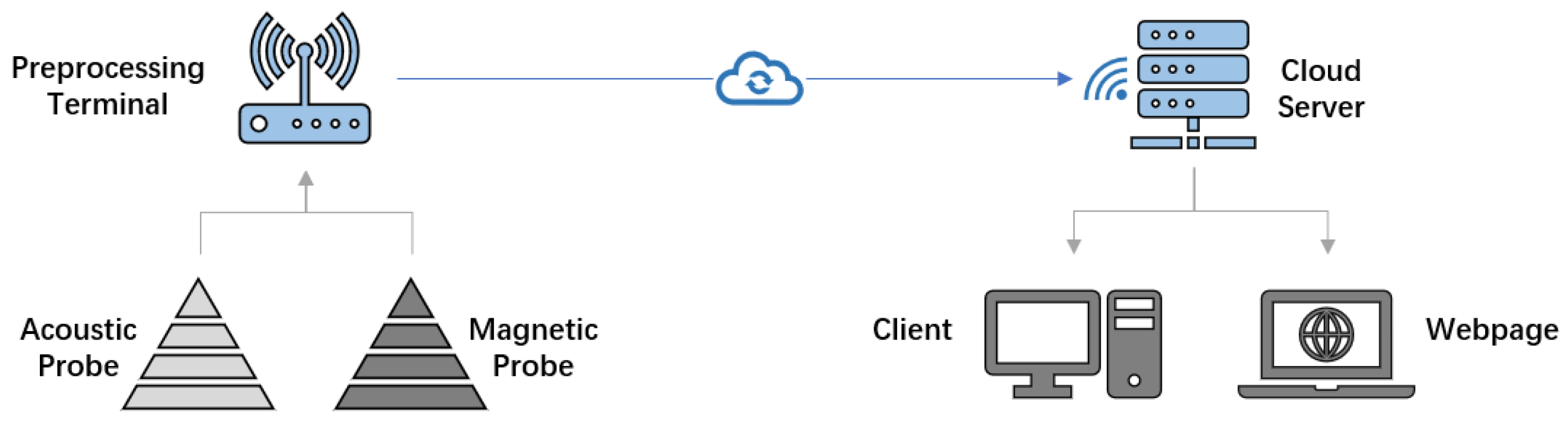
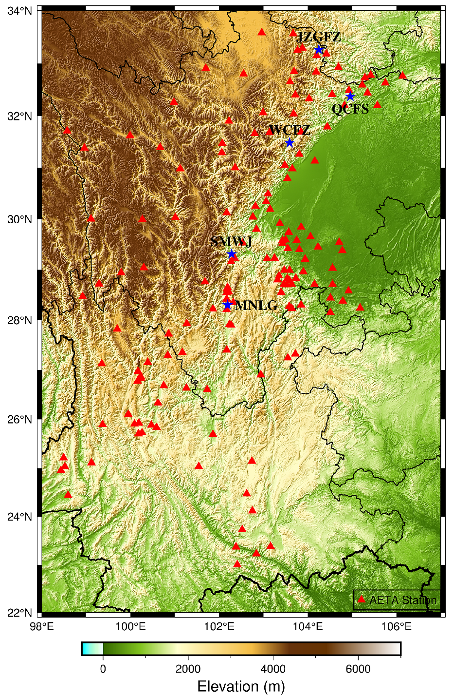
Although the ultra-low frequency electromagnetic anomalies have shown significant relation with earthquakes, there is still no work to monitor it in the long term and over a large area. However, earthquake precursor anomalies are generally long-term processes, so there is a large space in such a research area. To explore the possibility of ultra-low frequency electromagnetic anomalies in the long term, we designed the AETA system and set about four hundred monitor stations around Sichuan and Yunan, and the area is about 800,000 ${\mathrm{km}}^2$. Figure 1 shows the whole system of AETA. One station of AETA consists of a probe and station devices, which are responsible for data processing tasks and data uploading tasks. The probe collects acoustic and magnetic signals and sends them to the station for the next step. The station will do some processing work that contains down-sampling and wave filtering; then, it sends them to the cloud server. Everyone could gain data through the webpage and API. (To access the public data, just view the website aeta.cn or https://dtvs.aeta.net/stations, or send an email to [email protected]. The last access of the database is 6 December 2021.) Figure 2 shows the distribution of AETA stations. The stations follow the distribution of fault zones in this area to catch anomalies as much as possible.

The electromagnetic disturbance probe has a frequency response range of 0.1 Hz∼10 kHz with an intensity range of 0.1 nT∼1000 nT. Its sensitivity is 20 mV/nT in the range of 0.1 Hz∼10 kHz, the data resolution is 18 bit, and the voltage resolution is 19.073 $\mathsf{\mu }$V. The high-frequency sampling rate of the probe is 30 kHz.

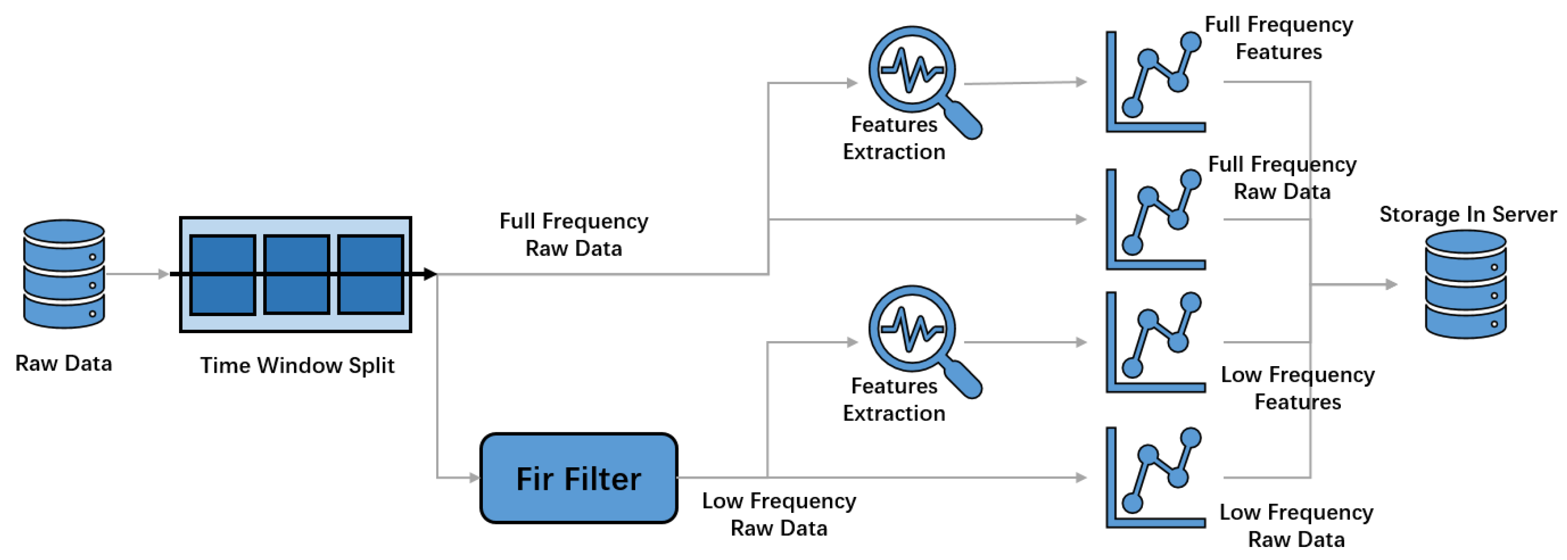
The energy of magnetic abnormal concentrates in ultra-low frequency [19,20,21]. According to this, we use a Butterworth filter to down-sample the raw data of 30 kHz to reduce the cost of data transmission and storage. The signal energy is concentrated below 250 Hz. According to the Nyquist sampling theorem [22], a sample rate $f_s$ could perfectly reconstruct a signal whose band limit is $f_s/2$, and the raw data will be down-sampled to 500 Hz, and this process saves information in the raw data under 250 Hz. The difference between the full frequency signal and the low-frequency signal is not obvious, and the signal energy is concentrated below 250 Hz. The seismic electromagnetic phenomenon is related to the rock fracture caused by the accumulation of underground stress and the electromagnetic radiation generated during the development of microcracks. This is more related to the ultra-low frequency signal below 30 Hz, and this frequency is less interfered with by other electromagnetic sources, so this frequency range is more valuable.

3.2. Data Preprocessing

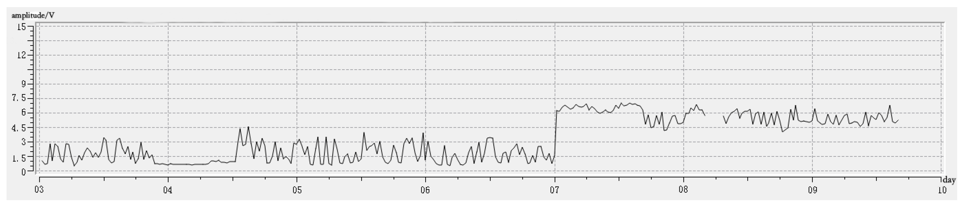
Figure 3 shows the data preprocessing work flow of AETA. In the cloud server, the raw data will be reduced to one value per minute according to Equation (1). The constants in Equation (1) are results of the device metadata of the Analog-to-Digital Converter (ADC). As Figure 4 showed, each point represents a minute, and the raw time-series data whose frequency is 500 Hz is reduced to a series data whose frequency is 1/60 Hz. These data are used to be the input of machine learning, and we call it the minute data.

$$MEAN=\frac{1}{30000}\sum _{i=1}^{30000}12.288\times \frac{\left|VALU{E}_i\right|}{32768}$$

(1)

The sliding window uses a constant length window to slide on the input series with a constant step to cut a series of sub-series and deal with the sub-series. We use the sliding window method to process the minute data; the window length is 60, and the step is also 60, so we average per hour to generate one number. In this way, one day will contain 24 values, and they will use as a vector of length 24 according to the chronological order, and the data become a series of vectors, in which each vector represents one day. The sliding window method is used to organize these vectors. Since the sun’s activity influences the local geomagnetic, a period window of 27 is used to reduce this influence, and the final input is a series of matrices $A_{24\times 27}$, in which 27 means the sun’s activity period and 24 means hours in one day.

4. PCA Extraction for Single Station

4.1. Introduction

The data are complex and full of noise and redundant information, which is the reason why a feature dimension reduction process is important. In our work, the effective information that is related to an earthquake is not obvious, making the noise reduction process more important. Dimension reduction could reduce noise in data. On the other hand, the complexity of common algorithms increases as $KlogK,K^2,K^3$, or $a^K$ when the dimension K increases. Therefore, reducing the dimension of the input data can greatly reduce the calculation cost.

PCA is an algorithm commonly used in dimension reduction and feature extraction. It could reduce the duplicate data, and it shows the main components of original input data.

4.2. PCA Algorithm of Single Station

Based on the assumption that local underground variation may cause some detailed changes of the local geomagnetic field, the analysis of the local AETA geomagnetic signal may capture earthquakes.

$$X={[X_1,X_2,X_3,\cdots ,X_n]}^T$$

(2)

$${\Sigma }_{ij}=cov(X_i,X_j)=E\left[(X_i-E\left[X_i\right])(X_j-E\left[X_j\right])\right]$$

(3)

$$\Sigma =E\left[(\mathit{X}-E\left[\mathit{X}\right]){(\mathit{X}-E\left[\mathit{X}\right])}^T\right]=\left[\begin{array}{cccc}cov(X_1,X_1)& cov(X_1,X_2)& \cdots & cov(X_1,X_n)\\ cov(X_2,X_1)& cov(X_2,X_2)& \cdots & cov(X_2,X_n)\\ ⋮& ⋮& \ddots & ⋮\\ cov(X_n,X_1)& cov(X_n,X_2)& \cdots & cov(X_n,X_n)\end{array}\right]$$

(4)

In the PCA algorithm, a co-variance matrix $\Sigma$ of matrix $A_{24\times 27}$. As Equation (2), for a multidimensional random variable X that is length n, the co-variance matrix is a symmetric matrix of $n\times n$, and the elements on the diagonal are the variances of the random variables in each dimension. For the $A_{24\times 27}$, its co-variance matrix is ${\Sigma }_{27\times 27}$. Element ${\Sigma }_{ij}$ in matrix $\Sigma$ is as Equation (3), so matrix $\Sigma$ is as Equation (4).

The procedure of the PCA algorithm is as follows:

1

Calculate the co-variance matrix $\Sigma$ of $A_{24\times 27}$;

2

Calculate the eigenvalue ${\lambda }_1,{\lambda }_2,\cdots ,{\lambda }_n$ of $\Sigma$ and the related eigenvector matrix $({\zeta }_1,{\zeta }_2,\cdots ,{\zeta }_n)$;

3

Choose K eigenvectors with the largest eigenvalues as row vectors and use the corresponding eigenvectors as row vectors of new matrix P. The K should be chosen to make the cumulative contribution eigenvector rate a of eigenvalue a more than 85%. The contribution is calculated as shown in Equation (5);

4

Take the eigenvector matrix P to reconstruct the original data matrix $A_{24\times 27}$; first, calculate the projection values of $A_{24\times 27}$ on these eigenvectors, and then inverse transform them to the original coordinate system to obtain the reconstruction matrix $A_{24\times 27}^{\prime }$;

5

Use the last line of the original data matrix $A_{24\times 27}$ to be vector L, which is related to the last day in 27 days and its length is 24, and use the last line of the reconstructed data matrix $A_{24\times 27}^{\prime }$ to be vector L${}^{\prime }$. Take the difference of the two vectors. Take the difference between the original data matrix $A_{24\times 27}$ and the related element of the last row of the reconstructed data matrix $A_{24\times 27}^{\prime }$ (the last day of the selected 27 days). Then, set all elements of this line to zero except the one with the largest absolute value. This will generate a vector named “feature vector” of length 24 as the eigenvector of the matrix $A_{24\times 27}^{\prime }$, and it is the output vector of this algorithm. In addition to this, the largest K eigenvalues are also output.

$$P_i=\frac{{\lambda }_i}{{\sum }_{m=1}^n{\lambda }_m}$$

(5)

This algorithm is suitable for our data, which have large information redundancy. The data matrix of one sample is a $24\times 27$ matrix, the 24 is related to 24 h per day, and the 27 is related to the 27 days of one sample according to the sun’s activity period. A PCA algorithm is used to extract the eigenvectors, which make up more than 85% of the energy and reconstruct them. The reconstructed matrix contains the main signals in the data matrix. After subtracting them from the original matrix, some subtle changes of the periodic signals will be captured.

Based on the matrix $A_{24\times 27}$ of each time step, we can get several features related to the last day of the 27 days of its time step. Based on the matrix of each $A_{24\times 27}$, we can get several features related to the last day of the 27 days. The features contain a vector generated in Step 5, which is called “feature vector”. The number of values is decided by K, and here are three: feature1, the first principal component; feature2, the second principal component; and feature3, the third principal component. These features will be used in the prediction model to represent each station itself.

Another feature is the proportion of the related eigenvalues of each principal component in the sum of all eigenvalues. We find that before an earthquake, the proportion of the first principal component often decreased and the proportion of the second and third principal components increased, so it can become a feature [23,24,25]. The first principal component may be related to the background signals caused by the local environment and geological structure, so it is a general data form. On another side, the second and third principal components may be related to pre-anomalies of an earthquake, which may be caused by seismic activity.

4.3. PCA Algorithm of Multiple Stations

Earthquake precursors are area processes, so the anomalies of one station before the earthquake may be related to its neighbor, and the data of a single station cannot catch this type of potential relevance between different stations. In this work, we use multi-station PCA to resolve these problems. Earthquakes are caused by the movement of the earth’s plates, and our work is based on a hypothesis that the rupture of the fault zone is regional, so the earthquake precursor may be captured and recorded by multiple stations at the same time.

We hypothesize that an area with low earthquake probability should have mild underground activities and the data of stations in this area should be similar. An earthquake is a regional event, and the data of stations in this area should be more different.

A PCA method such as that in Section 4.2 is as follows. Firstly, use a sliding window of length 27 to slide on the time series data processed in Section 3.2; for station A, it is $Ro{w}_{1\times 27}^A$; for station B, it is $Ro{w}_{1\times 27}^B$, and so on. Stack the vectors to organize the time-series data to be a matrix: for example, two $1\times 27$ vectors will become a $2\times 27$ vector. In this step, matrix $M_{n\times 27}$ is output, and n is the number of used stations.

Secondly, use method in Section 4.2 to calculate the co-variance matrix of $M_{n\times m}$ and to get the eigenvalue ${\lambda }_1,{\lambda }_2,\cdots ,{\lambda }_n$ (from large to small) and their related eigenvector ${\xi }_{\mathbf{1}},{\xi }_{\mathbf{2}},\cdots ,{\xi }_{\mathbf{n}}$. In this work, m is 27 days. The eigenvalues ${\lambda }_1,{\lambda }_2,\cdots ,{\lambda }_n$ (from large to small) are called the first principal component, the second principal component, and so on.

We believe that the first principal component represents the similarity between stations, and the second principal component represents the difference. Based on this hypothesis, if an abnormal rise of the proportion of the second principal component appears, it indicates that the data of the two stations have unusual differences, which may be related to earthquakes.

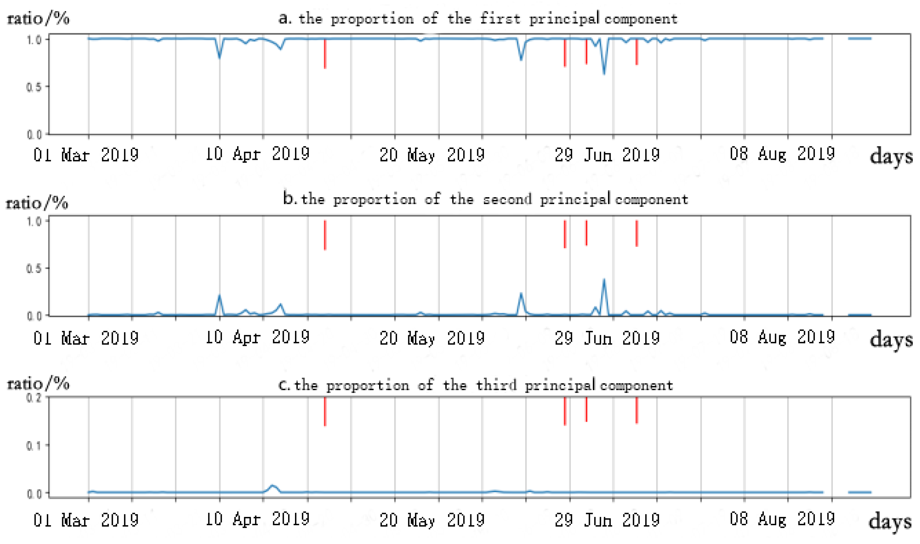
A measure named $E_s$ is used to measure the impact of earthquakes on a certain region, which is widely used in the research of Hayakawa and other seismologists [26]. Equation (6) shows the calculation method of this measure, in which M is the magnitude of the earthquake and R is the distance from earthquake to the station, $E_s^{\prime }$ is the influence of that one earthquake, and $E_s$ is the whole influence in one day. The previous methods such as that of Li Jiankai [12] set the stations’ number used in one matrix as 3. Figure 5 shows this three-station PCA features WCFZ (103.59${}^{\circ }$ E, 31.48${}^{\circ }$ N), JZGFZ (104.25${}^{\circ }$ E, 33.26${}^{\circ }$ N), and QCFS (104.96${}^{\circ }$ E, 32.37${}^{\circ }$ N) from 1 March 2019 to 18 August 2019. The red line represents all earthquakes whose $E_s$ values are greater than $5\times {10}^7$ around stations, including Sichuan Liangshan 3.3 at $(103.{35}^{\circ }\mathrm{E},28.{08}^{\circ }\mathrm{N})$ on 24 April 2019, Sichuan Yibin 5.3 at $(104.{89}^{\circ }\mathrm{E},28.{37}^{\circ }\mathrm{N})$ on 18 June 2019, Sichuan Yibin 5.4 at $(104.{77}^{\circ }\mathrm{E},28.{43}^{\circ }\mathrm{N})$ on 22 June 2019, and Sichuan Yibin 4.8 at $(104.{85}^{\circ }\mathrm{E},28.4^{\circ }\mathrm{N})$ on 3 July 2019. There always peaks behind earthquake markers every half a month, and there are no earthquakes during the time of the flat part. The first principal component may represent the similarity between stations, and the second principal component may represent the difference. The third principal component is usually flat and unimportant, and it will cost hundreds of times of consumption to calculate it because the numbers of the principal components (eigenvalues) of the input matrix can not be higher than the dimension of input in the PCA algorithm. In our experiment, the number of stations of each matrix is 2.

$$E_s^{\prime }=\frac{{10}^{4.8+1.5M}}{R^2},E_s=\sum _{1day}{E}_s^{\prime }$$

(6)

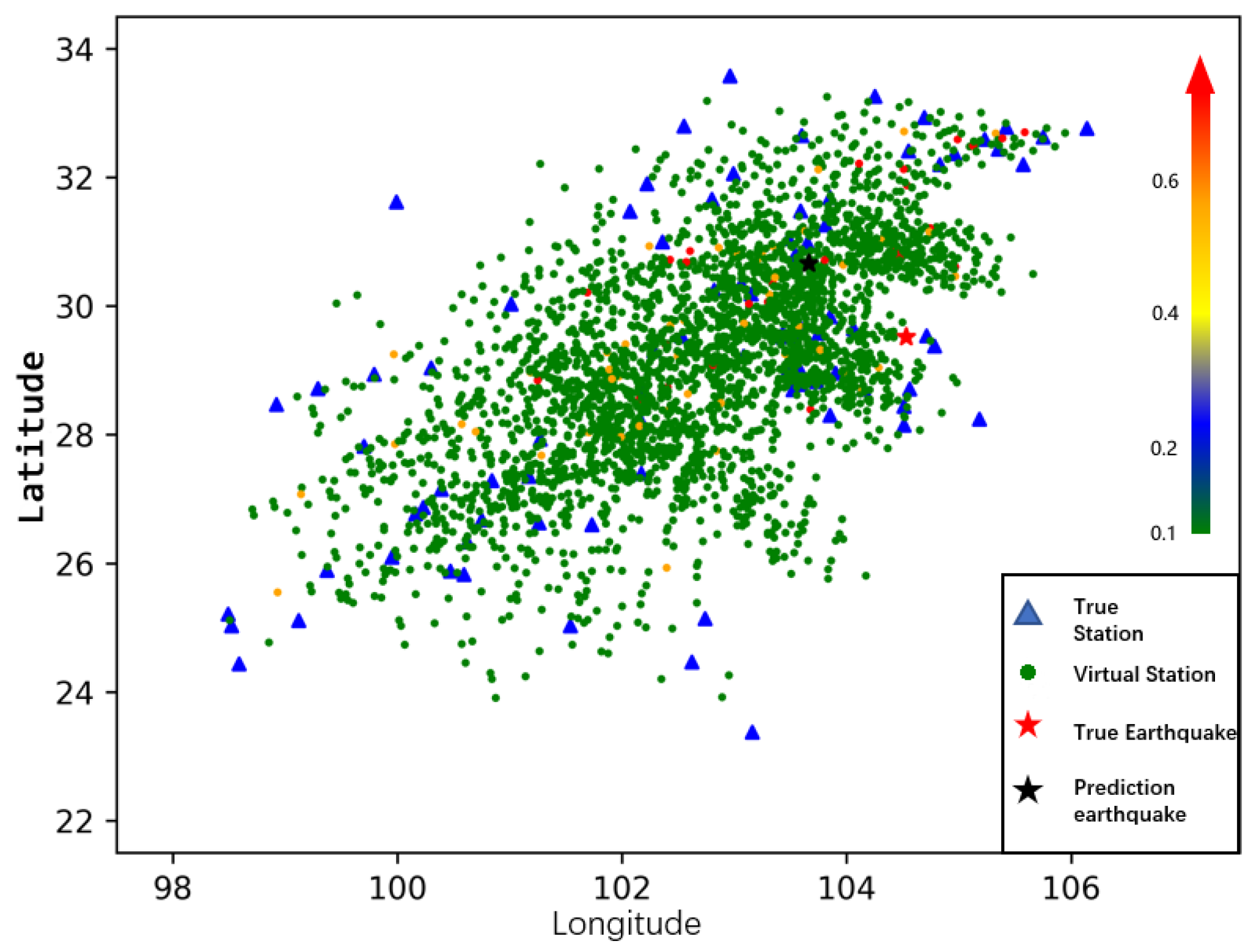
The two-stations method is used to extract the potential relationship between multiple stations, which is different from the single station method and expands the number of available points. The first principal component and the second principal component are features of two stations, and they are located at the center of the two stations. Figure 6 is an example of the first principal component feature. This area of this example is ${98}^{\circ }\mathrm{E}$ to ${107}^{\circ }\mathrm{E}$, ${22}^{\circ }\mathrm{N}$ to ${34}^{\circ }\mathrm{N}$, the time is from 12 September 2020 to 9 October 2020, and we use the last day, 9 October 2020, to represent the time.

Each virtual station in this image is the geometric center of a couple of two stations, and its color is related to the first principal component. The geometric center of all points that are above 0.6 will be regarded as the potential earthquake center, and this is our future method to locate the epicenter, while it is not used in this work.

In summary, the two-stations method works on two stations; we use the sliding method, whose window is 27 days, to cut data, stack two vectors to compute the covariance matrix, and use a PCA method to extract the features. Its output is two eigenvalues, named the first principal component and the second principal component, and their eigenvectors. The eigenvalues will be used as features in our model. The corresponding position of features is the center of two stations, which is called the virtual station. For an area that contains K stations, the number of virtual stations is $K(K-1)$.

5. Earthquake Prediction Model

5.1. Model Structure

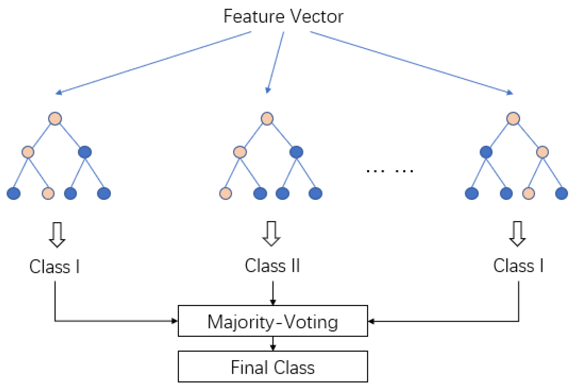
This work uses LightGBM (LGB) to predict the existence of earthquakes. LGB is a kind of implementation of Gradient Boosting Decision Tree (GBDT) [11,27,28], which is a semi-automatic machine learning model with good performance. LGB is often used to be a final prediction layer that summarizes features and generates a prediction. First, it generated multiple classifiers, and then, it combines them. Each sub-classifier has multiple layers, each layer has multiple nodes, which represents a possible property, and the whole classifier looks like a tree. Figure 7 shows this structure. This model selects split features by Gini coefficients at each node, trains a series of base classifiers based on the idea of gradient boosting, and considers all base classifiers together when making predictions.

The model focuses on the earthquake existence of an area, its input is a series of features extracted from the virtual stations in this area. A typical area usually contains about 20∼40 real stations, so it contains 400∼1600 virtual stations. We define a threshold V and all the virtual stations’ first principal components, which are under the threshold, and its corresponding second principal components will be used to calculate the input features. The granularity of output of the single-station PCA method and two-stations PCA method is individual days. For one week, we have 7 days, in which each day has its single-station PCA method and two-stations PCA method outputs. The output of the two-stations PCA method requires the following process, and the abnormal value is the first principal components value, which is under the threshold V:

1.

Use the mean values $V_{mean}^1$ of the abnormal values and the mean values $V_{mean}^2$ of the second principal components to be a part of features, and the station used to obtain the second principal components is the same as the abnormal values. Each day means every day should compute its mean value of all the abnormal values independently, and this step gets 14 values;

2.

The percentage $V_{per}^1$ of abnormal values in all values and the percentage $V_{per}^2$ of the second principal components of the same virtual stations. Each day means every day should compute its mean value of all the abnormal values independently, and this step gets 14 values;

3.

The number of abnormal values $V_N$ each day. This step gets seven values;

4.

Choose the three biggest values as the features of the first principal component of the single-station method for each day; this step get 21 values;

5.

Concatenate all the values and the single-station method output to be a vector whose length is $14+14+7+21=56$.

An area usually has ∼20–40 stations, and each sample which is a vector with a length of 56 is related to 7 days data. In addition to the input vector with a length of 56, the model needs its corresponding label for training. The label of each 7-day window is marked by the earthquake in its area. For a 7-day window, we choose the biggest earthquake magnitude in the next 7 days after the last day of data as the label, and the relationship of label and magnitude is as follows:

1.

No earthquake is marked as 0;

2.

Ms0–Ms3.5 is marked as 1;

3.

Ms3.5–Ms4.0 is marked as 2;

4.

Ms4.0–Ms4.5 is marked as 3;

5.

Ms4.5–Ms5.0 is marked as 4;

6.

Ms5.0–Ms5.5 is marked as 5.

5.2. Experiment

In this work, the used area is a rectangle in ${98}^{\circ }$ E∼106.2${}^{\circ }$ E and 28.1${}^{\circ }$ N∼34${}^{\circ }$ N. The time range of the training data set is from 1 July 2019 to 1 March 2021, and the time range of the testing data set is from 1 March 2021 to 31 December 2021. The distribution of data is shown in

Table 1. Table shows the distribution of samples in the data set.

Label	Level	Number in TrainSet	Number in TestSet
0	No Earthquake	209	25
1	Ms0+∼Ms3.5	184	12
2	Ms3.5∼Ms4.0	120	11
3	Ms4.0∼Ms4.5	50	13
4	Ms4.5∼Ms5.0	35	2
5	Ms5.0+	11	6
Total		609	69

. The corresponding earthquakes of the testing data set are listed in

Table 2. Table shows earthquakes used to evaluate the model.

Time	Magnitude/Ms	Latitude/North	Longitude/East
1 March 2021 18:13	3.8	26	100
19 March 2021 18:57	3.9	31.93	104.2
5 May 2021 9:51	3.6	32.4	104.02
13 May 2021 11:42	4.7	24.43	99.24
18 May 2021 21:39	4.2	25.65	99.93
19 May 2021 20:05	4.4	25.66	99.92
21 May 2021 20:56	4.2	25.63	99.93
21 May 2021 21:21	5.6	25.63	99.92
21 May 2021 21:23	4.5	25.66	99.97
21 May 2021 21:48	6.4	25.67	99.87
21 May 2021 21:53	4.1	25.62	99.98
21 May 2021 21:55	5	25.67	99.89
21 May 2021 21:56	4.9	25.64	99.95
21 May 2021 22:02	4.1	25.66	99.89
21 May 2021 22:03	3.9	25.57	99.93
21 May 2021 22:15	4	25.59	99.96
21 May 2021 22:31	5.2	25.59	99.97
21 May 2021 22:59	3.5	25.63	99.94
21 May 2021 23:13	3.8	25.64	99.94
21 May 2021 23:22	3.5	25.66	99.88
21 May 2021 23:23	4.5	25.6	99.98
22 May 2021 0:51	4	25.7	99.87
22 May 2021 1:36	3.5	25.62	99.94
22 May 2021 2:28	3.9	25.62	99.91
22 May 2021 3:14	3.6	33.74	100.93
22 May 2021 9:48	4	25.67	99.9
22 May 2021 20:14	4.4	25.61	99.93
27 May 2021 19:52	4.1	25.74	99.95
27 May 2021 23:03	3.6	25.69	99.89
10 June 2021 19:46	5.1	24.34	101.91
10 June 2021 19:58	3.6	24.37	101.92
14 June 2021 4:02	3.8	31.98	104.48
16 June 2021 15:35	4.2	24.33	101.91
20 June 2021 11:31	3.8	22.65	100.33
23 June 2021 5:11	3.8	32.2	104.94
28 June 2021 19:48	4.6	24.31	101.89
29 June 2021 6:41	3.6	25.75	99.99
5 July 2021 5:48	4	32.92	99.02
7 July 2021 4:19	4.2	28.05	104.99
14 July 2021 23:36	4.8	30.97	103.37
21 July 2021 3:01	3.6	27.42	103.08
23 July 2021 14:22	3.7	32.61	102.19
23 July 2021 20:55	4.1	29.28	105.44
25 July 2021 0:23	3.9	32.62	102.16
4 August 2021 19:12	4.8	23.38	106.71
21 August 2021 10:20	4.5	27.12	105.31
1 September 2021 6:37	3.7	28.11	105.1
3 September 2021 21:30	4.8	28.09	104.92
11 September 2021 15:05	4.3	23.39	106.71
16 September 2021 4:33	6	29.2	105.34
24 September 2021 4:08	3.6	28.07	105.06
18 October 2021 8:37	4.3	29.26	103.96
10 November 2021 16:39	3.9	29.59	104.69
12 November 2021 9:50	4.3	28.08	105.09
16 November 2021 13:22	4.8	22.31	101.68
16 November 2021 15:54	4.6	22.31	101.69
21 November 2021 18:51	4.6	28.45	104.79
24 November 2021 17:16	4.6	26.87	106.68
1 December 2021 5:39	4.2	28.34	104.97
10 December 2021 19:25	3.7	28.12	105.14
24 December 2021 21:43	6	22.33	101.69
24 December 2021 22:02	4.9	22.33	101.66
31 December 2021 22:53	4.8	22.35	101.67

, while their number is 63. The corresponding stations are listed in

Table 3. Stations used in the experiment.

Station ID	Longitude	Latitude	StationID	Longitude	Latitude
19	103.65	30.98	183	105.35	32.44
26	102.17	30.12	184	102.99	32.06
33	102.28	29.31	198	104.83	32.2
38	102.17	28.55	204	103.81	31.26
43	105.23	32.59	221	103.06	30.34
47	104.51	28.15	228	104.9292	32.48778
48	104.79	28.38	240	103.85	29.84
73	103.54	28.83	247	102.53	29.53
75	103.94	29.21	250	103.48	31.05
77	104.51	28.44	251	106.14	32.76
87	103.08	29.22	252	102.96	33.58
93	102.82	30.25	255	103.43	29.52
94	101.01	30.03	256	103.43	29.58
96	103.25	29.23	302	103.4	28.55
98	102.22	31.9	303	99.79	28.94
99	104.16	31.13	307	103.46	28.71
105	103.5	29.59	308	98.92	28.47
107	102.36	31	309	102.1895	28.29901
115	105.75	32.63	310	103.1011	30.48795
116	104.55	32.41	313	100.3	29.04
121	104.25	33.26	315	103.32	28.8
122	100.67	31.39	316	103.47	28.99
124	103.15	30.19	317	103.59	28.99
133	99.99	31.62	321	104.15	28.71
141	105.42	32.78	324	104.71	29.54
148	103.9	28.96	328	104.06	29.65
150	104.96	32.37	329	103.55	29.42
159	103.54	30.79	331	104.23	29.45
167	103.72	32.4	334	103.57	29.74
170	102.06	31.29	335	104.78	29.38
172	104.69	32.93	339	104.56	28.71
177	102.84	29.8	355	105.18	28.24
181	102.1678	28.20821

. The sliding window time step of the training data is 1 day, and the sliding window time step of the testing data is 4 days. If magnitude Ms3.5 is regarded as the threshold of positive and negative, the number of positive samples in the train set is 393, the number of negative samples in the train set is 216, the number of positive samples in the test set is 37, and the number of negative samples in the test set is 32. The distribution of train set and test set is different especially in earthquakes whose magnitudes are beyond 4.5, such as the Ms6.4 earthquake on 21 May 2021 and its aftershocks, which are shown in Table 2. The difference is a big challenge for the generalization performance of the model and shows the complexity of earthquake prediction.

It is easy to find that the data are unbalanced from Table 1, so we expand the unique labels 3, 4, and 5 in the train data by copying them into the train data several times. Label 3 is copied one time, label 4 is copied three times, and label 5 is copied five times.

The LightGBM algorithm is a machine learning algorithm with lots of super parameters that need to be set up manually, and the best values according to the experiment need to be chosen as well. In this work, the super parameters that we changed include the learning rate (Lr), Num-leaves, and max-depth. Lr is a super parameter that controls the speed of updating internal parameters of the model, Num-leaves and max depth control the complexity of the model. Generally, a bigger Lr means faster and rough updating, and a bigger Num-leaves and bigger max-depth mean a more complex model. We use the grid search method, which generates all possible super parameter combinations and tests them one by one. Lr is chosen from [0.0001, 0.001, 0.01, 0.1, 0.5], Num-leaves is chosen from [3, 5, 8, 12, 16, 20], and max-depth is chosen from [3, 5, 8, 12, 16, 20, 25].

In the experiment, we use a random train set to run a control group experiment. To ensure the authenticity of the data, the random data share the same source with the true train set, which is not shuffled, and the relationship between data and label is shuffled. This random train set is trained in the same environment of true train set and super parameters and will be evaluated in the same test set. The final super parameters that we used are as follows: Lr is ${10}^{-5}$, max-depth is 12, and num-leaves is 20.

5.3. Results Analysis

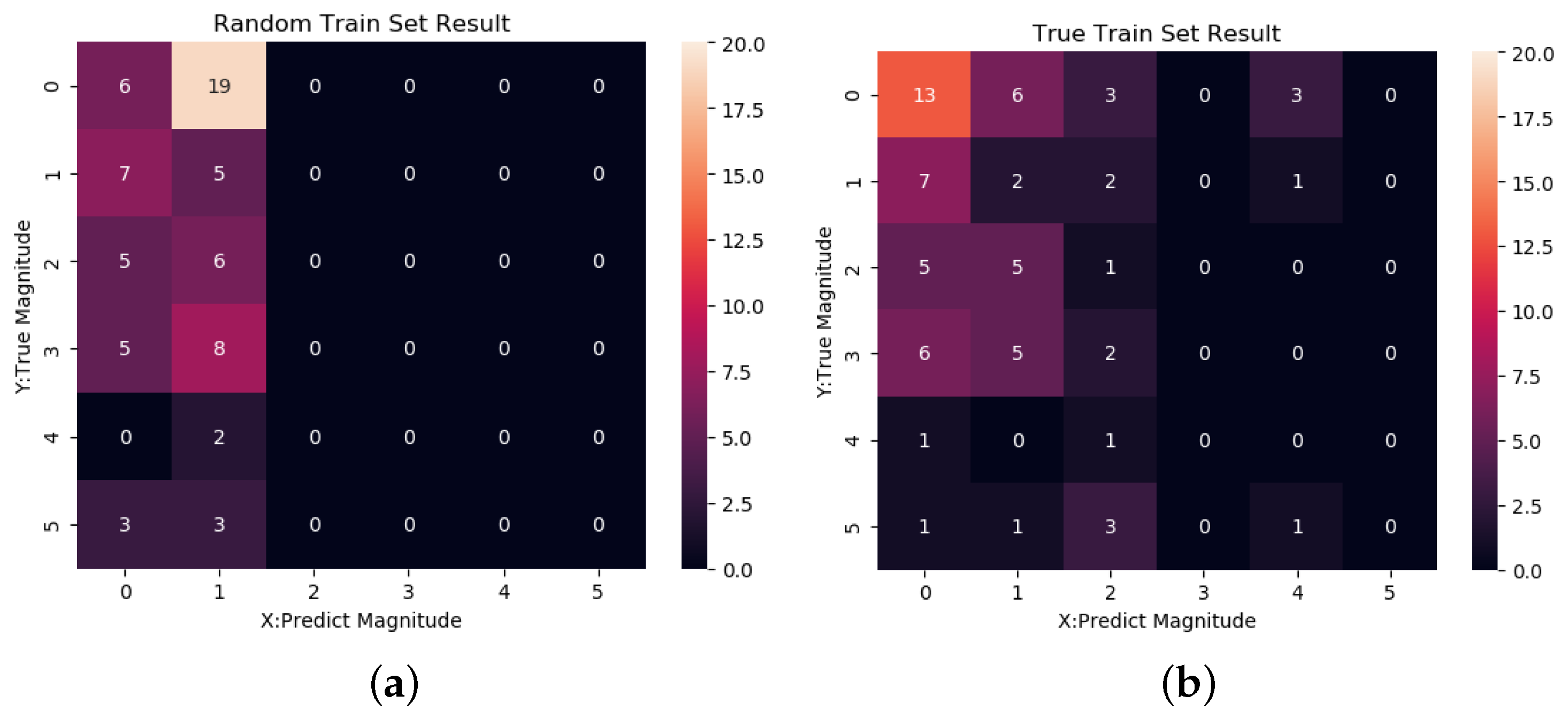
We use heat maps to visualize the data, as Figure 8 shows. Each number in the heat map means a class in which the true magnitude is the x-axis and the predicted magnitude is the y-axis. For example, in the position (0, 1) true set results, the number is 7, which means that in the 69 samples of the test set, there are seven events in which the events have 0 labels (meaning there is no earthquake) and the model gives 1 label (meaning it believes that an earthquake under Ms3.5 should happen). On the diagonal, the predicted magnitude and the true magnitude are equal, which means that it is a full right prediction, and the further the prediction is from the diagonal, the greater the deviation between the predicted and true value. In the random results map, 11 samples are on the diagonal, while 16 samples are on the diagonal in the true map. The random set model gives 19 negative samples’ positive predictions whose magnitudes are around Ms3.5 and six negative samples’ negative predictions, while the true set models give 12 negative samples’ positive predictions and 13 negative samples’ negative predictions. In addition, the random model has no ability to give positive predictions, because the relationship is broken by shuffle, and it can only give label 0 and label 1, which are more numerous. However, the model trained on true data (called true model) can give some meaningful results.

Accurately distinguishing the magnitude of two nearby labels is hard, because the train samples are not enough and unbalanced, the earthquake is complex, and the theory is not developed. To give a more intuitive prediction of whether there is an earthquake or not, we choose a threshold to determine the output of the model. In Section 5.2, we use Ms3.5 to be the threshold of positive and negative.

Table 4. Binary results of true model and random model.

Model	Precision	Recall	f1-Score	Accuracy
True Model	0.25	0.471	0.327	0.522
Random Model	0	0	0	0.536

shows the precision, recall, F1-score, and accuracy of the positive–negative binary results of the two models. Precision means the ratio of right positive samples in all the predicted positive samples, recall means the ratio of the right positive samples in all the true positive samples, and the f1-score is their geometric mean. Accuracy means the ratio of all right predictions. There is no big gap between the two models’ accuracy, but the F1-score of the random model is 0 because it can only give a negative prediction, as Figure 8 shows. However, the true model could predict some true earthquakes even though there is a gap between their magnitude, which means that the model truly learns something from the data.

The true model has 198 sub-trees, the random model has 30,000 sub-trees, and each tree is more complex than the true model. We think that it is because the data and label in the random train set are shuffled, and the model over fits on it, making a model with poor generalization ability.

5.4. Further Work

A better model of earthquake prediction should be built from the following aspects:

1.

Increasing data accumulation;

2.

Using more effective features besides PCA features because it can only describe a part of the earthquake precursors;

3.

Using a complex model, a better model may extract more of the relationship between features and events.

6. Conclusions

In our work, we raise an earthquake prediction model based on data accumulated by the AETA system to achieve certain results. We prove that there is a correlation between the AETA data and earthquakes around the AETA stations.

There are still some improvements that could be applied. As a result of the uneven distribution of the AETA stations, the epicenter location still has a bias problem, which then leads to a low-accuracy prediction. On the other hand, the feature that we extracted from the AETA data is insufficient, and we believe that the next work should focus on other features and combine these features to build a better model.

References

- Yong, S.; Xu, B.; Liang, Y.; Bai, Z.; An, H.; Zhang, X.; Huang, J.; Xie, Z.; Lin, K.; He, C. Research and Implementation of Multi-component Seismic Monitoring System AETA. Beijing Da Xue Xue Bao 2018, 54, 487–494. Available online: https://caod.oriprobe.com/articles/53135156/Design_and_Implementation_of_Signal_Processing_in_.htm (accessed on 6 December 2021).
- Jin, X.-R.; Yong, S.-S.; Wang, X.-A.; Pang, R.-T.; Han, C.-X.; Zeng, J.-W. Design and Implementation of Signal Processing in Seismic Monitoring System AETA. Computer Technology and Development. 2018, pp. 45–50. Available online: http://en.cnki.com.cn/Article_en/CJFDTotal-WJFZ201801010.htm (accessed on 6 December 2021).
- Felzer, K.R. Calculating the Gutenberg–Richter b value. In Proceedings of the AGU Fall Meeting, San Francisco, CA, USA, 11–15 December 2006. [Google Scholar]
- Santis, A.D.; Cianchini, G.; Favali, P.; Beranzoli, L.; Boschi, E. The Gutenberg-Richter law and entropy of earthquakes: Two case studies in Central Italy. Bull. Seismol. Soc. Am. 2011, 101, 1386–1395. [Google Scholar]
- Sornette, D.; Sornette, A. General theory of the modified Gutenberg-Richter law for large seismic moments. Bull. Seismol. Soc. Am. 1999, 89, 1121–1130. [Google Scholar]
- Cicerone, R.D.; Ebel, J.E.; Britton, J. A systematic compilation of earthquake precursors. Tectonophysics 2009, 476, 371–396. [Google Scholar]
- Rikitake, T. Earthquake precursors. Bull. Seismol. Soc. Am. 1975, 65, 1133–1162. [Google Scholar]
- Rikitake, T. Earthquake precursors in Japan: Precursor time and detectability. Tectonophysics 1987, 136, 265–282. [Google Scholar]
- Chen, Y.-T.; Gu, H.-D.; Lu, Z.-X. Variations of gravity before and after the Haicheng earthquake, 1975, and the Tangshan earthquake, 1976. Phys. Earth Planet. Inter. 1979, 18, 330–338. [Google Scholar]
- Brodsky, E.E.; Lay, T. Recognizing foreshocks from the 1 April 2014 Chile earthquake. Science 2014, 344, 700–702. [Google Scholar]
- Ke, G.; Meng, Q.; Finley, T.; Wang, T.; Chen, W.; Ma, W.; Ye, Q.; Liu, T.Y. Lightgbm: A highly efficient gradient boosting decision tree. Adv. Neural Inf. Process. Syst. 2017, 30, 3146–3154. [Google Scholar]
- Jiankai, T.J.L. Principal component analysis and local correlation tracking as tools for revealing and analyzing seismo-electromagnetic signal of earthqauke. Seismol. Geol. 2017, 39, 517–535. [Google Scholar]
- Guo, Q.; Yong, S.; Wang, X. Statistical Analysis of the Relationship between AETA Electromagnetic Anomalies and Local Earthquakes. Entropy 2021, 23, 411. [Google Scholar]
- Bin, Z.; Jinyun, G.; Xiaotao, C. Analysis of TEC anomalies before earthquake based on principal component analysis and the sliding inter quartile range method. GNSS World China 2016, 41, 63–69. Available online: http://en.cnki.com.cn/Article_en/CJFDTOTAL-QUDW201604014.htm (accessed on 6 December 2021).
- Lv, Y.; Wang, X.; Huang, J.; Yong, S. Research on Jiuzhaigou Ms 7.0 Earthquake Based on AETA Electromagnetic Disturbance. Acta Sci. Nat. Univ. Pekin. 2019, 55, 1007–1013. [Google Scholar]
- Yao, X.-Y.; Feng, Z.-S. Review on the recent development of analysis methods on magnetic disturbance associated with earthquakes. Prog. Geophys. 2018, 33, 511–520. [Google Scholar]
- Zhang, J.; Liu, X.; Yao, L.; Ma, X.; Yuan, Y.; Yin, X. Study on Anomalous Change Characters of Electromagnetic Disturbance before the Wenchuan Ms 8.0 Earthquake. Seismological and Geomagnetic Observation and Research. Available online: http://en.cnki.com.cn/Article_en/CJFDTOTAL-DZGJ201005010.htm (accessed on 6 December 2021).
- Jiang, F.; Chen, X.; Zhan, Y.; Zhao, G.; Yang, H.; Zhao, L.; Qiao, L.; Wang, L. Shifting Correlation Between Earthquakes and Electromagnetic Signals: A Case Study of the 2013 Minxian–Zhangxian ML 6.5 (MW 6.1) Earthquake in Gansu, China. Pure Appl. Geophys. 2016, 173, 269–284. [Google Scholar]
- Frase Smith, A.C.; Bernardi, A.; McGill, P.R.; Ladd, M.E.; Helliwell, R.A.; Villard, O.G., Jr. Low frequency magnetic field measurements near the epicenter of the Ms 7.1 Loma Prieta earthquake. Geophys. Res. Lett. 1990, 17, 1465–1468. [Google Scholar]
- Merzer, M.; Klemperer, S.L. Modeling low-frequency magnetic-field precursors to the Loma Prieta earthquake with a precursory increase in fault-zone conductivity. Pure Appl. Geophys. 1997, 150, 217–248. [Google Scholar]
- Fraser-Smith, A.C.; McGill, P.R.; Helliwell, R.A.; Villard, O.G., Jr. Ultra-low frequency magnetic field measurements in Southern California during the Northridge earthquake of 17 January 1994. Geophys. Res. Lett. 1994, 21, 2195–2198. [Google Scholar]
- Shannon, C.E. Communication in the presence of noise. Proc. IRE 1949, 37, 10–21. [Google Scholar]
- Wold, S.; Esbensen, K.; Geladi, P. Principal component analysis. Chemom. Intell. Lab. Syst. 1987, 2, 37–52. [Google Scholar]
- Zhu, K.; Li, K.; Fan, M.; Chi, C.; Yu, Z. Precursor Analysis Associated With the Ecuador Earthquake Using Swarm A and C Satellite Magnetic Data Based on PCA. IEEE Access 2019, 7, 93927–93936. [Google Scholar]
- Chi, C.; Zhu, K.; Yu, Z.; Fan, M.; Li, K.; Sun, H. Detecting Earthquake-Related Borehole Strain Data Anomalies With Variational Mode Decomposition and Principal Component Analysis: A Case Study of the Wenchuan Earthquake. IEEE Access 2019, 7, 157997–158006. [Google Scholar]
- Hattori, K.; Serita, A.; Yoshino, C.; Hayakawa, M.; Isezaki, N. Singular spectral analysis and principal component analysis for signal discrimination of ULF geomagnetic data associated with 2000 Izu Island Earthquake Swarm. Phys. Chem. Earth Parts A/B/C 2006, 31, 281–291. [Google Scholar]
- Friedman, J.H. Greedy function approximation: A gradient boosting machine. Ann. Stat. 2001, 29, 1189–1232. [Google Scholar]
- Chen, T.; Guestrin, C. Xgboost: A scalable tree boosting system. In Proceedings of the 22nd ACM Sigkdd International Conference on Knowledge Discovery and Data Mining, San Francisco, CA, USA, 13–17 August 2016; pp. 785–794. [Google Scholar]
Figure 1.
AETA system contains probe, station, server and UI of client and webpage.
Figure 2.
Distribution of AETA stations in Sichuan province in China. The stations used in next section are marked by blue stars, and positions of other stations marked by red triangles.
Figure 3.
Workflow of the process of AETA raw data.
Figure 4.
MNLG low-frequency electromagnetic feature.
Figure 5.
Multi-PCA features; red line means earthquake. The stations used in this figure, WCFZ, JZGFZ, and QCFS, are shown in Figure 2. (a–c) shows the first, second, and third principal component.
Figure 6.
Multi-PCA map. The red star is the earthquake, and the black star is the predicted epicenter. Green points are virtual stations, which are located at the center of two stations.
Figure 7.
The structure of LightGBM model (LGB). LGB is a kind of implementation of Gradient Boosting Decision Tree that is widely used in various machine learning tasks.
Figure 8.
Evaluated results on true set and random set. (a) Random set results; (b) True set results.