Filtering Properties of Discrete and Continuous Elastic Systems in Series and Parallel

Abstract

Filtering properties and local energy distribution in different classes of periodic micro-structured elastic systems are analysed in this work. Out-of-plane wave propagation is considered in continuous and discrete elastic systems arranged in series and parallel. Filtering properties are determined from the analysis of dispersion diagrams and energy distribution within different phases in the representative unit cell. These are determined analytically by implementing a transfer matrix formalism. The analysis given in the work indicates quantitatively how to couple phases, having discrete and continuous nature, in order to tune wave propagation and energy localisation.

1. Introduction

It is well known that infinite periodic structures behave as filtering systems. In such media, the Floquet–Bloch analysis evidences that there are some ranges of frequencies where, in absence of dissipation, waves propagate without attenuation, while, in the remaining frequency ranges, waves decay exponentially, with a decay exponent that can reach values not achievable by dissipative effects. Such frequency intervals are addressed as pass bands and stop bands, respectively. This well-known filtering effect has been recognised in various fields, such as acoustics, optics, elastic waves [1] and electromagnetic waves [2].

Filtering properties of periodic systems have been investigated in the vibration of crystal lattices [3] and widely applied in engineering designs, including electrical, acoustic and mechanical filters [4,5], microwave transformers and waveguides [6,7], periodically layered structures [8,9], and beams [10], plates [11,12] and membranes [13] with periodic supports.

If the system is finite, the wave propagation does not exactly obey the Bloch waveform and numerical solutions of the wave response have been computed by traditional matrix methods [14], two-way state-flow graph method [15] and eigenfunctions symmetries [16]. The results of the Floquet–Bloch waves in periodic systems can be conveniently applied to finite systems and, therefore, to real structures, exhibiting similar transmission properties [17,18], even for a small number of repetitive units [19]. In such a case, it is more correct to denote the frequency intervals as propagation and non-propagation ranges. Note also that, in real structures, defect and imperfections in the structural porperties can introduce a ‘disorder’, which, within a certain range, slightly alters the dispersion properties of a system [20], especially in the acoustical branches [21].

Dispersion analysis for elastic lattices [22,23,24,25] evidences that the discrete nature of the elastic system gives rise to dispersion, namely a nonlinear relation between the frequency and the wave vector, where the number of bands is associated with the number of Lagrangian coordinates within the unit cell. In such systems, special properties, such as wave beaming and occurrence of band gaps, are achieved by varying periodically the stiffness and the density of the lattice components [26,27]. Parenthetically, another source of dispersion comes from the geometry and boundary conditions, as in Structural Mechanics, where, starting from the three-dimensional continuum theory and following an asymptotic procedure, structural models like in beams, plates or shells are obtained, which are dispersive. Well-known examples are flexural waves in plates and beams or Lamb waves (see, for example, [28]). Applications combining structural models and periodic systems include periodic lattices composed of Rayleigh beams [29,30], resonant metawedge due to rods on the boundary of an half-space [31] and gyroscopic beams periodically attached to a plate [32,33].

In three-dimensional continuous systems, dispersion is generated by heterogeneities, which can be, for example, in the form of laminates [34,35] or inclusions in particulate composites, addressed as photonic crystals when the microstructure is periodic [36,37]. Dispersion of elastic waves in continuous systems with prestress was discussed in [38,39] and in structured media in [40,41].

For mono-dimensional periodic structures, different analytical and numerical techniques were proposed in order to apply Floquet–Bloch conditions using the superposition principle in the linear regime [42]. Analytically, the transfer matrix approach was applied in [43,44,45] and the quasi-periodic dynamic Green’s function in [19,46]. Alternatively, the semi-analytical Rayleigh–Ritz method from a variational formulation was presented in [47,48]; if the geometry is more complicated or additional finer details need to be embedded in the model, the Floquet–Bloch condition can be implemented numerically in Finite Element packages (see, for example, the nice application to a real bridge in [49]).

Analytical models are in general more difficult to implement, but they can clearly identify the influence of different structural parameters on the dispersion properties. The quasi-periodic Green’s function is a very elegant formalism, but the application to problems governed by the Helmholtz type of equations has the drawback that the Green’s function is singular at the origin [46], while, for flexural problem governed by the biharmonic fourth-order equation, the Green’s function is bounded at the origin [19] and singularities identify the bounds for the dispersion curves corresponding to a homogeneous structures (see the ‘light lines’ in [50]). The transfer matrix can be obtained both analytically and numerically and has the property to maintain the same size when different units are connected, since internal variable are automatically eliminated. It has been given in analytical form for quite complicated structures in [51] and for quasi-crystals where the distribution of the internal microstructures follow different Fibonacci sequences [52,53].

In this work, we propose a transfer matrix formalism, with the aim of combining units with discrete and continuous nature; in addition, we analyse the effect of arranging different units in series and parallel. Due to the nature of the dynamic problem, the non-hermitian transfer matrix belongs to a symplectic space and its eigenvalues are reciprocal if real, and complex conjugated with unit modulus otherwise [43,44,45]. Parenthetically, the properties of the transfer matrix can also be evaluated in the invariant space, where, due to energy conservation, the determinant is one and the number of independent invariants is half of the even dimension of the matrix itself. In our case, the matrix has dimension 2 and it is sufficient to evaluate only the trace to determine the dispersion relation. Such simplification gives the possibility to easily identify the dispersive effects of different structural parameters, which are analysed in detail in the present work.

The research extends the previous analyses performed in [41,45], by considering a problem governed by the Helmholtz operator in which the microstructure is arranged both in series and in parallel. The arrangement in series proposed here is a generalisation of the model proposed in [41]. The continuous and discrete character is not trivial and dates back to the concept of structural or structured interface, which was introduced in a seminal work [40] and applied in the elastostatic regime [54,55,56] to denote a structural element that involves non-local interactions. The discrete character is a result of a proper asymptotic approximations that was developed in [57] and a nice application on the homogenisation of damage in an elongated structure can be found in [21]. The scope of the work is the description of the filtering properties and energy distribution for wave propagation in periodic elastic structures having a discrete and continuous character and arranged in series and parallel. The description of the filtering properties is obtained from the inspection of dispersion diagrams, while the final investigation describes the energy distribution within different components of the unit cell. The parametric analysis developed here shows which are the mechanical parameters that govern the band distribution for different arrangements and nature of the phases. Particular attention is devoted to internal resonators, which play an important role in several applications [58,59]. The parametric analysis also evidences the conditions for which a highly localised effect is obtained and the possibility to have multiple localised resonances.

In Section 2, we define the transfer matrices for continuous and discrete units and for different combinations in series and parallel. The single components of the transfer matrices for all cases is reported in Appendix A. Dispersion relations and the corresponding behaviours are analysed in Section 3, where, in normalised form, the parametric analysis in terms of frequency and elastic impedance ratios is detailed. In Section 4, the energy distribution in different units is studied, while concluding remarks are given in the Conclusions, Section 5.

2. Materials and Methods

Antiplane shear waves are considered, in the time-harmonic regime with radian frequency $\omega$. At normal incidence the spatial distribution $U\left(x\right)$ of the displacement component $u(x,t)=U\left(x\right)e^{-i\omega t}$, along the z-axis perpendicular to the propagation direction x, satisfies the Helmholtz-type equation of motion:

$$\frac{d^{2}U\left(x\right)}{d{x}^2}+\frac{{\omega }^2}{c^2}U\left(x\right)=0,c=\sqrt{\frac{\mu }{\rho }},$$

(1)

where $\mu$ is the shear modulus of the linear elastic isotropic medium and $\rho$ its density (note that the Helmholtz equation also describes low frequency waves in a rod. For longitudinal waves, U is the longitudinal displacement and $c=\sqrt{E/\rho }$, with E being the Young’s modulus; for torsional waves, U is the angle of twist and $c=\sqrt{\mu /\rho }$). The wave form can be expressed in terms of complex amplitudes A and B as:

$$U\left(x\right)=A{e}^{ikx}+B{e}^{-ikx},k=\omega /c,$$

(2)

where k is the wavenumber.

In a homogeneous layer of thickness d, located between the initial coordinate $x_0$ and the final coordinate $x_1=x_0+d$, displacements satisfying Equation (1) and corresponding tractions $\tau \left(x\right)=\mu \partial U/\partial x$ at points $x_0$ and $x_1$ are related by means of the unimodular transfer matrix M $=\left[m_{ij}\right]$. Collecting displacement and traction in the generalised displacement vector $\mathbf{v}\left(x\right)={\left[U\left(x\right)\tau \left(x\right)\right]}^T$, within a unit cell:

$$\mathbf{v}\left(x_1\right)=\mathbf{M}\mathbf{v}\left(x_0\right),$$

(3)

or, explicitly:

$$\left(\begin{array}{c}U\left(x_1\right)\\ \tau \left(x_1\right)\end{array}\right)=\left[\begin{array}{cc}{m}_{11}& m_{12}\\ m_{21}& m_{22}\end{array}\right]\left(\begin{array}{c}U\left(x_0\right)\\ \tau \left(x_0\right)\end{array}\right).$$

(4)

In the following, we compute the explicit form of the transfer matrix for different interface configurations. First, we show the transfer matrix for a single layer or unit of continuous or discrete nature; then, we couple the transfer matrices of the single layers to obtain the global matrix for systems composed of units arranged in series or in parallel.

2.1. Single Unit Transfer Matrix

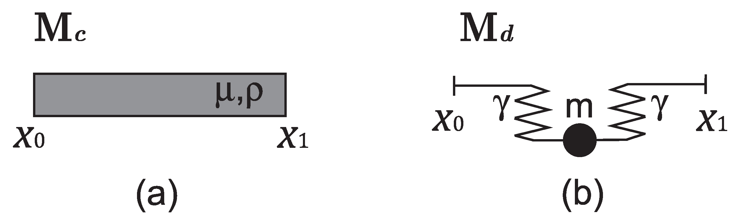
For the continuous layer of Figure 1a, the transfer matrix takes the form [60]:

$${\mathbf{M}}_c=\left[\begin{array}{cc}{\displaystyle cos\varphi }& {\displaystyle \frac{1}{Q}sin\varphi }\\ {\displaystyle -Qsin\varphi }& {\displaystyle cos\varphi }\end{array}\right],$$

(5)

where $\varphi =kd$ is the phase increment, d the layer thickness and $Q=k\mu$.

The transfer matrix for the discrete system given in Figure 1b is [41]:

$${\mathbf{M}}_d=\left[\begin{array}{cc}{\displaystyle \frac{\gamma -m{\omega }^2}{\gamma }}& {\displaystyle \frac{2\gamma -m{\omega }^2}{{\gamma }^2}}\\ -m{\omega }^2& {\displaystyle \frac{\gamma -m{\omega }^2}{\gamma }}\end{array}\right].$$

(6)

As a consequence of the symplectic structure of the problem, energy conservation implies that the transfer matrices are unimodular; such a property holds also for more complex elastic systems. Therefore, the evaluation of only the first invariant of $\mathbf{M}$, i.e., the trace, will be sufficient to determine the dispersion properties.

2.2. Transfer Matrix for Units in Series and Parallel

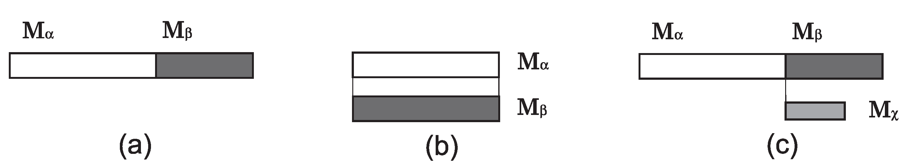
We combine now in three different ways the single units described in the previous Section: in particular, we consider configurations in series (Figure 2a), in parallel (Figure 2b) and the special one described in Figure 2c. For simplicity, we indicate with:

$${\mathbf{M}}_i=\left[\begin{array}{cc}{m}_{11}^{\left(i\right)}& m_{12}^{\left(i\right)}\\ m_{21}^{\left(i\right)}& m_{22}^{\left(i\right)}\end{array}\right],i=\alpha ,\beta ,\chi$$

(7)

the single unit transfer matrix.

For the systems shown in Figure 2a, with two units arranged in series, the global transfer matrix is simply obtained by multiplying single unit matrices [60], namely:

$${\mathbf{M}}_S={\mathbf{M}}_{\beta }{\mathbf{M}}_{\alpha }=\left[\begin{array}{cc}{m}_{11}^{\left(\alpha \right)}{m}_{11}^{\left(\beta \right)}+m_{21}^{\left(\alpha \right)}{m}_{12}^{\left(\beta \right)}& m_{12}^{\left(\alpha \right)}{m}_{11}^{\left(\beta \right)}+m_{22}^{\left(\alpha \right)}{m}_{12}^{\left(\beta \right)}\\ m_{11}^{\left(\alpha \right)}{m}_{21}^{\left(\beta \right)}+m_{21}^{\left(\alpha \right)}{m}_{22}^{\left(\beta \right)}& m_{12}^{\left(\alpha \right)}{m}_{21}^{\left(\beta \right)}+m_{22}^{\left(\alpha \right)}{m}_{22}^{\left(\beta \right)}\end{array}\right].$$

(8)

If the single units $\alpha$ and $\beta$ are disposed in parallel as in Figure 2b, the corresponding matrix ${\mathbf{M}}_P$ has components:

$$\begin{array}{ccc}\hfill m_{11}^{\left(P\right)}& =& \frac{m_{11}^{\left(\alpha \right)}{m}_{12}^{\left(\beta \right)}+m_{12}^{\left(\alpha \right)}{m}_{11}^{\left(\beta \right)}}{m_{12}^{\left(\alpha \right)}+m_{12}^{\left(\beta \right)}},\hfill \\ \hfill m_{12}^{\left(P\right)}& =& \frac{m_{12}^{\left(\alpha \right)}{m}_{12}^{\left(\beta \right)}}{m_{12}^{\left(\alpha \right)}+m_{12}^{\left(\beta \right)}},\hfill \\ \hfill m_{21}^{\left(P\right)}& =& \frac{(m_{12}^{\left(\alpha \right)}+m_{12}^{\left(\beta \right)})(m_{21}^{\left(\alpha \right)}+m_{21}^{\left(\beta \right)})-(m_{11}^{\left(\alpha \right)}-m_{11}^{\left(\beta \right)})(m_{22}^{\left(\alpha \right)}-m_{22}^{\left(\beta \right)})}{m_{12}^{\left(\alpha \right)}+m_{12}^{\left(\beta \right)}}\hfill \\ \hfill & =& \frac{m_{12}^{\left(\alpha \right)}{m}_{21}^{\left(\beta \right)}+m_{21}^{\left(\alpha \right)}{m}_{12}^{\left(\beta \right)}+m_{11}^{\left(\alpha \right)}{m}_{22}^{\left(\beta \right)}+m_{22}^{\left(\alpha \right)}{m}_{11}^{\left(\beta \right)}-2}{m_{12}^{\left(\alpha \right)}{m}_{12}^{\left(\beta \right)}},\hfill \\ \hfill m_{22}^{\left(P\right)}& =& \frac{m_{22}^{\left(\alpha \right)}{m}_{12}^{\left(\beta \right)}+m_{12}^{\left(\alpha \right)}{m}_{22}^{\left(\beta \right)}}{m_{12}^{\left(\alpha \right)}+m_{12}^{\left(\beta \right)}}.\hfill \end{array}$$

(9)

The transfer matrix for the structured system of Figure 2c can be computed by considering the three single units, $\alpha$, $\widehat{\chi }$, $\beta$, in series, i.e., ${\mathbf{M}}_T={\mathbf{M}}_{\beta }{\widehat{\mathbf{M}}}_{\chi }{\mathbf{M}}_{\alpha }$, where ${\widehat{\mathbf{M}}}_{\chi }$ can be computed from the components of the transfer matrix ${\mathbf{M}}_{\chi }$ of the unit $\chi$ in the following manner:

$${\widehat{\mathbf{M}}}_{\chi }=\left[\begin{array}{cc}1& 0\\ {\displaystyle \frac{m_{21}^{\left(\chi \right)}}{m_{22}^{\left(\chi \right)}}}& 1\end{array}\right].$$

(10)

Needless to say, it is trivial to check that ${\mathbf{M}}_S$, ${\mathbf{M}}_P$ and ${\mathbf{M}}_T$ are unimodular.

3. Results

In Brun et al. [41], following [60,61], it has been shown how to make use of the transfer matrix approach to study the dispersion properties of periodic elastic systems. In particular, we consider a micro-structured system made up of a repetition of a certain unit cell and we apply the Floquet–Bloch condition $\mathbf{v}\left(x_1\right)=e^{i\varphi }\mathbf{v}\left(x_0\right)$, where $\varphi =kd$ is the Floquet–Bloch parameter, k is the wave number and d is the total length of the unit cell.

Remembering that $\mathbf{v}\left(x_1\right)=\mathbf{M}\mathbf{v}\left(x_0\right)$, the condition $\det (\mathbf{M}-e^{i\varphi }\mathbf{I})=0$, with $\mathbf{I}$ the identity matrix, gives the dispersion relation. By taking advantage of the unimodularity of $\mathbf{M}$, in order to obtain the dispersion relation, it is sufficient to compare the trace of the transfer matrix of the unit cell with the trace of the transfer matrix of an equivalent homogeneous layer with a transfer matrix in the form of Equation (5).

3.1. Two Continuous Layers in Series

First, we consider a two-layer continuous system with a unit cell matrix given by Equation (8), with ${\mathbf{M}}_{\alpha }={\mathbf{M}}_1$ and ${\mathbf{M}}_{\beta }={\mathbf{M}}_2$, as in Equation (5); the dispersion relation takes the form:

$$cos\varphi =cos\left(\frac{d_1}{c_1}\omega \right)cos\left(\frac{d_2}{c_2}\omega \right)-\frac{1}{2}\left(\frac{Q_1}{Q_2}+\frac{Q_2}{Q_1}\right)sin\left(\frac{d_1}{c_1}\omega \right)sin\left(\frac{d_2}{c_2}\omega \right),$$

(11)

where the subscripts 1 and 2 indicate the two continuous phases. Relation (11) corresponds to the equation obtained by Bigoni and Movchan [40] (their Equation (38), in which their parameter $dh$ is now $\varphi$) and by Brun et al. [41] (their Equation (14)).

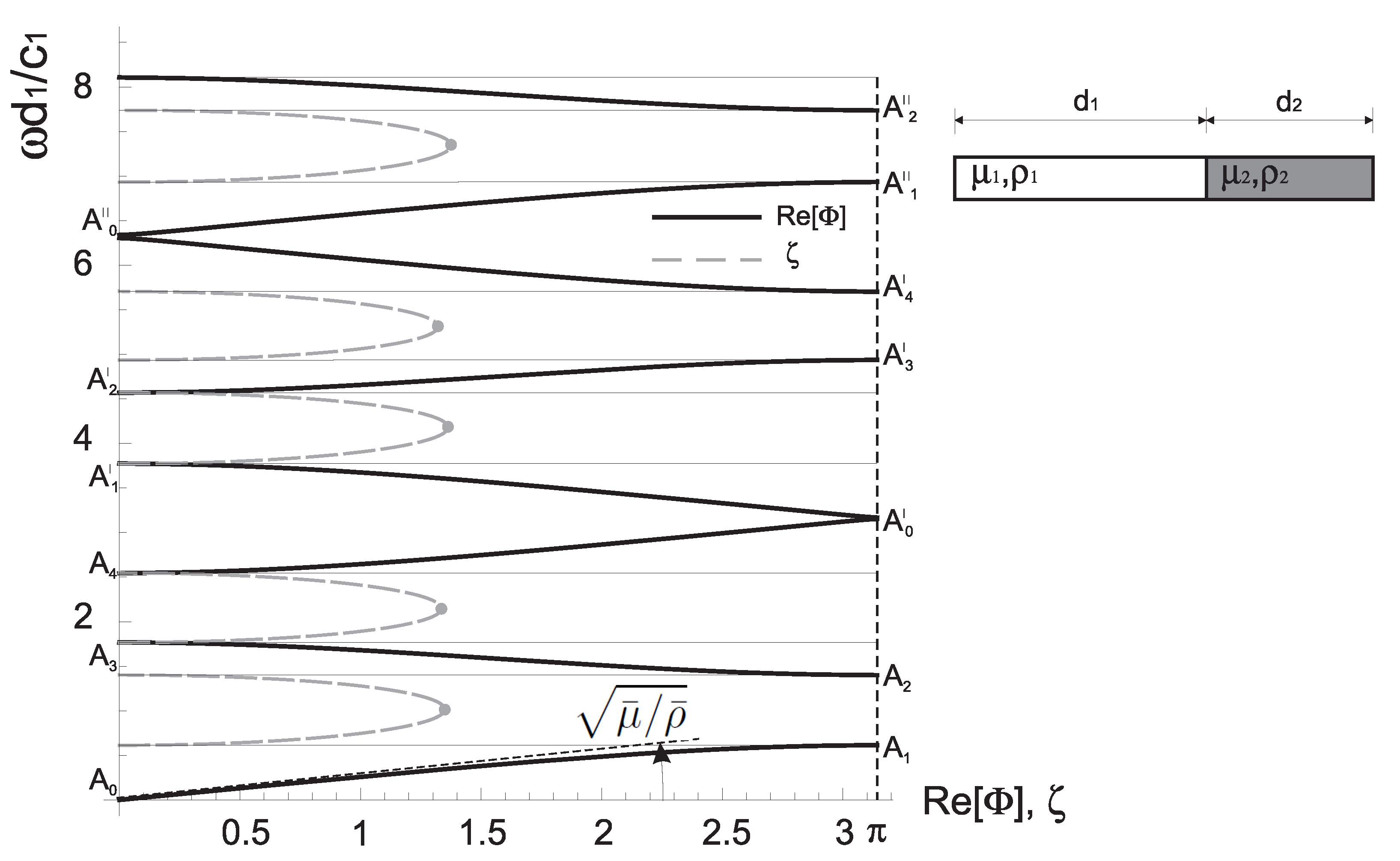
The dispersion relation (11) is shown in Figure 3 (diagrams have been created in Wolfram Mathematica (version 12.0)). It presents propagating and no-propagating bands in which the group velocity $\partial \omega /\partial k$ can be either positive or negative. In Equation (11), $\varphi$ plays the role of the Floquet–Bloch parameter, so that the nature of the solution changes from pass band when $\varphi$ is real, that is for $|cos\varphi |\le 1$ and $\left|\mathrm{tr}\mathbf{M}\right|\le 2$, to stop band when $\varphi$ is complex, that is for $|cos\varphi |>1$ and $\left|\mathrm{tr}\mathbf{M}\right|>2$. When $\varphi$ is complex, we take $\varphi =\pi -i\zeta$ or $\varphi =i\zeta$ ($\zeta >0$), where $\zeta =log\left(\right|cos\varphi |+\sqrt{{cos}^2\varphi -1})$ is the decay exponent of the exponentially decaying solution.

In the quasi static limit, for $\omega \to 0$ and $k\to 0$, the structured medium appears to be non dispersive with homogenised phase and group velocity both equal to $\sqrt{\overline{\mu }/\overline{\rho }}$, where:

$$\overline{\mu }=\frac{{\mu }_1{\mu }_2}{d_1{\mu }_2+d_2{\mu }_1}d\mathrm{and}\overline{\rho }=\frac{d_1{\rho }_1+d_2{\rho }_2}{d},$$

(12)

are the homogenised shear modulus and mass density, respectively, with $d=d_1+d_2$. Note that the homogenised shear modulus and mass density are equal to the harmonic and arithmetic means, respectively, of the phases values.

We introduce now the homogenised characteristic frequency:

$$\overline{\omega }=\sqrt{\frac{\overline{\mu }}{\overline{\rho }}}\frac{1}{d},$$

(13)

which contains the length-scale factor d; correspondingly, we define the characteristic frequencies:

$${\omega }_1=\sqrt{\frac{{\mu }_1}{{\rho }_1}}\frac{1}{d_1},{\omega }_2=\sqrt{\frac{{\mu }_2}{{\rho }_2}}\frac{1}{d_2},$$

(14)

having ratio ${\eta }_c={\omega }_1/{\omega }_2$ and the following elastic impedances:

$$q_1=d_1\sqrt{{\mu }_1{\rho }_1},q_2=d_2\sqrt{{\mu }_2{\rho }_2},$$

(15)

having ratio ${\xi }_c=q_1/q_2$, so that the quantities $|ln{\eta }_c|$ and $|ln{\xi }_c|$ measure the contrast between the two phases. Then, the dispersion relation (11) can be recast in the adimensional form:

$$cos\varphi =\frac{1}{4}\frac{{(1+{\xi }_c)}^2}{{\xi }_c}cos{\varphi }_{+}-\frac{1}{4}\frac{{(1-{\xi }_c)}^2}{{\xi }_c}cos{\varphi }_{-},$$

(16)

where:

$$\begin{array}{c}\hfill \Omega =\frac{\omega }{\overline{\omega }},\delta =\sqrt{1+{\eta }_c^2+\left({\xi }_c+\frac{1}{{\xi }_c}\right){\eta }_c},\frac{\omega }{{\omega }_1}=\frac{\Omega }{\delta },\\ \hfill {\varphi }_{+}=\frac{1+{\eta }_c}{\delta }\Omega ,{\varphi }_{-}=\frac{1-{\eta }_c}{\delta }\Omega .\end{array}$$

(17)

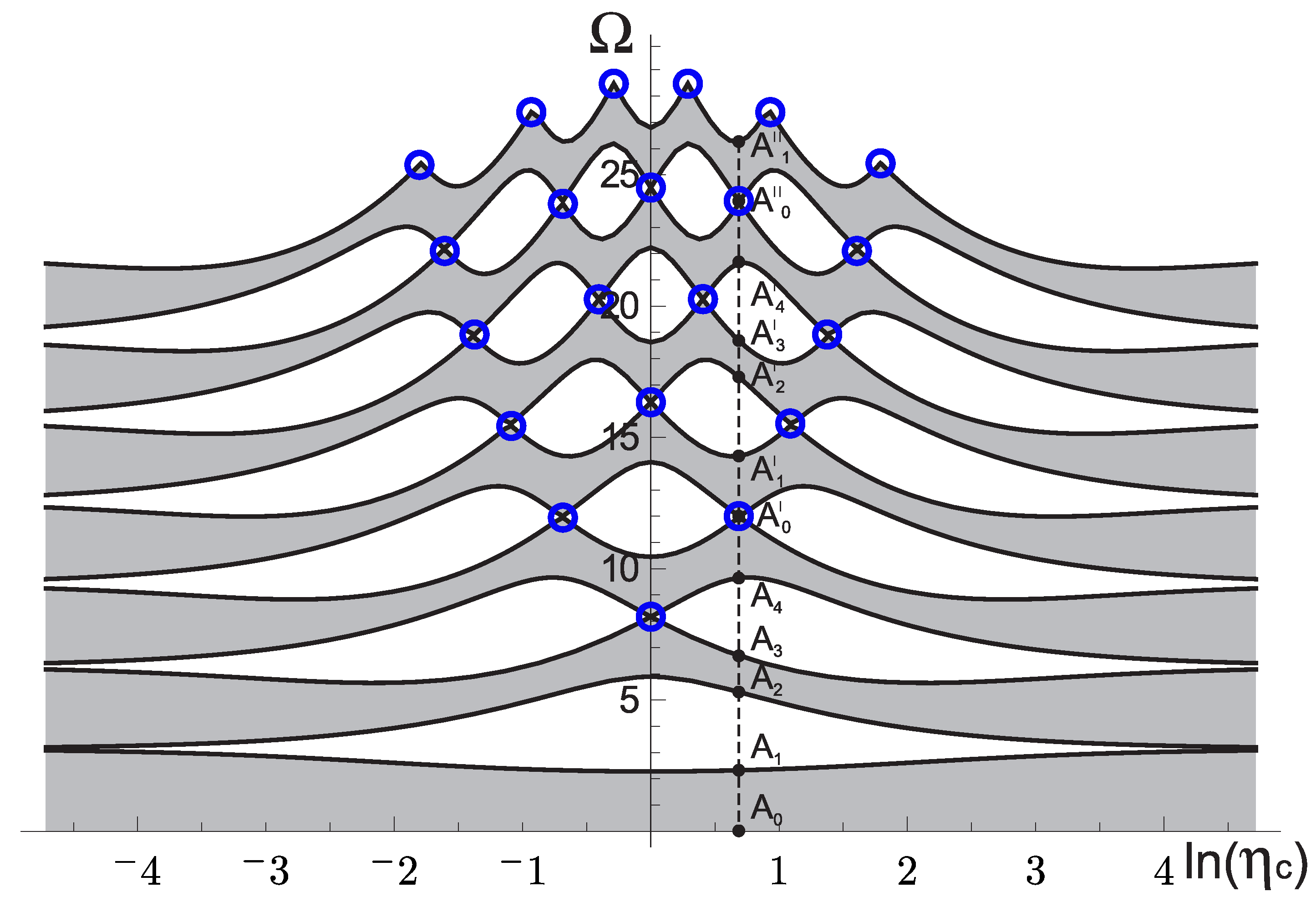
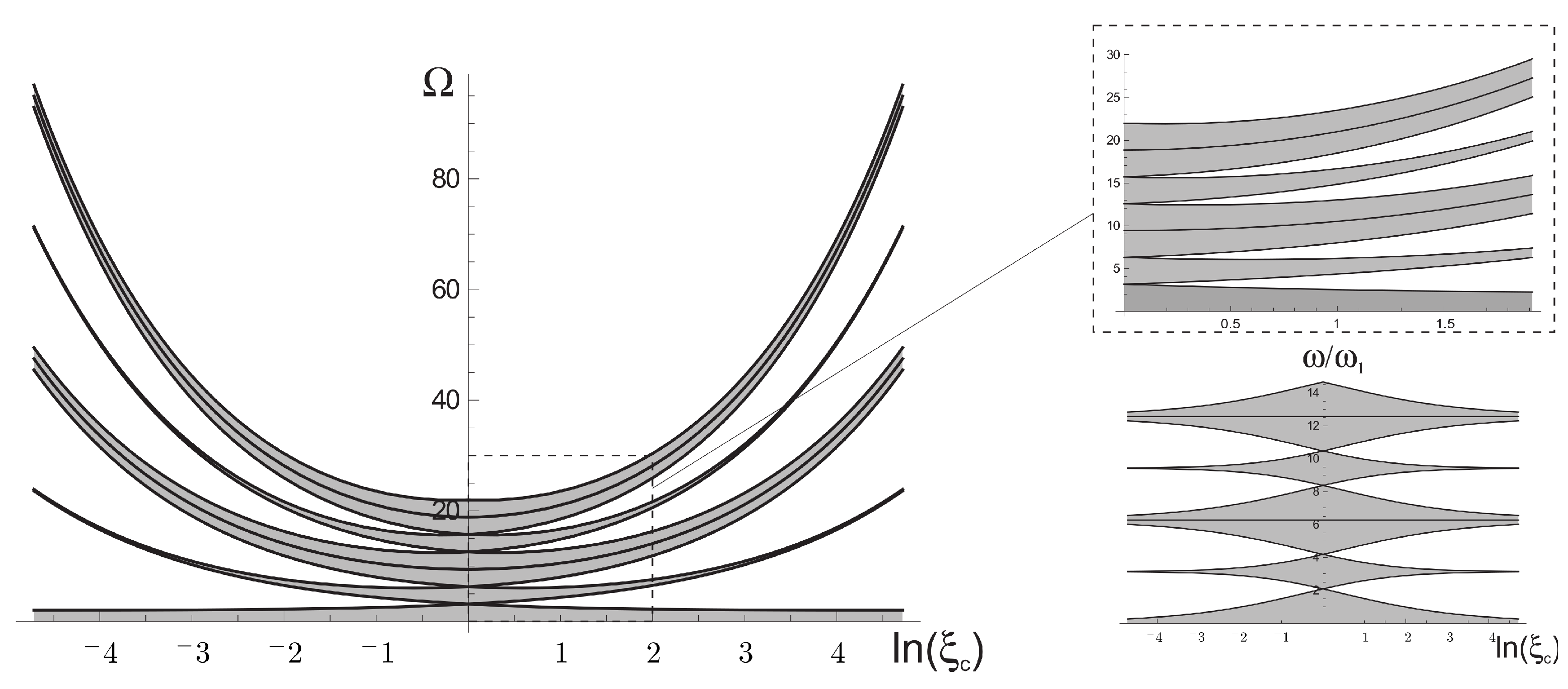
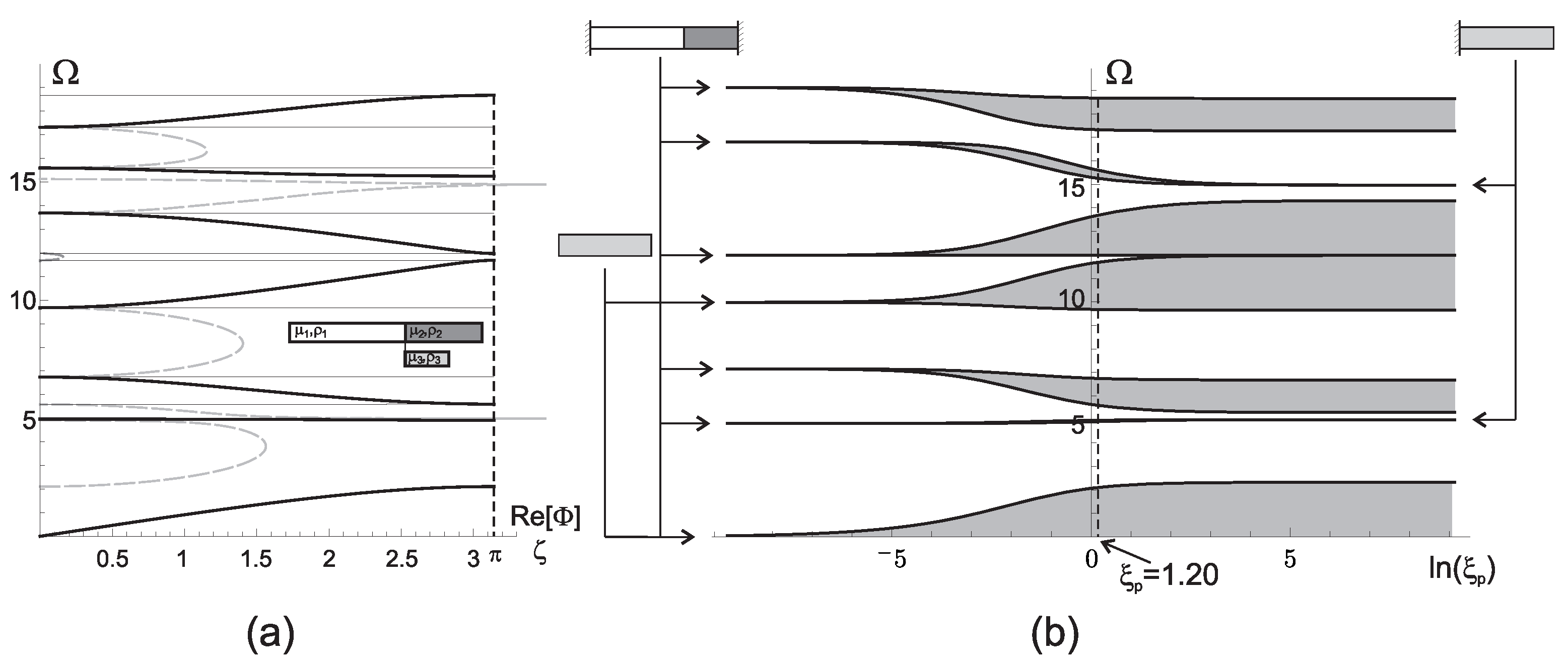
In Figure 4 and Figure 5, the frequency distribution of the bands is analysed as a function of the frequency ratio ${\eta }_c$ and impedance ratio ${\xi }_c$, respectively. The first seven bands are given in grey in Figure 4 for the impedance ratio ${\xi }_c=0.22$ and in Figure 5 for the characteristic frequency ratio ${\eta }_c=0.5$.

The diagrams are symmetric with respect to $ln{\eta }_c=0$ and $ln{\xi }_c=0$, respectively, and it is evident that there is a not-monotonic dependence of the band frequencies on the ratio ${\eta }_c$.

When ${\eta }_c=1$ ($ln{\eta }_c=0$), despite the fact that the phases have the same characteristic frequency, dispersion, identified by the presence of stop and pass bands, is due to the impedance mismatch (i.e., ${\xi }_c\ne 1$).

Note that:

$$\underset{{\eta }_c\to 0,\infty }{lim}\frac{1+{\eta }_c}{\delta }=\underset{{\eta }_c\to 0,\infty }{lim}\frac{|1-{\eta }_c|}{\delta }=1,$$

(18)

implying ${\varphi }_{+},{\varphi }_{-}\to \Omega$, so that the right-hand side of the dispersion Equation (16) reduces to $cos\Omega$. Therefore, for extreme characteristic frequency contrast between the phases, the dynamic behaviour of the laminate tends to be non dispersive with homogenised shear modulus and mass density given in Equation (12). In approaching this limiting values of ${\eta }_c$, narrowing pass bands are localised around frequencies $\Omega =n\pi$, $n\in {\mathcal{N}}_0$ (see Figure 4 for large $|ln{\eta }_c|$).

The right-hand side of Equation (16) is a periodic function of $\Omega$ if the ratio $(1+{\eta }_c)/(1-{\eta }_c)$ is rational; periodicity points are the contact points between different bands highlighted with blue circles in Figure 4. For example, if we pose the attention on the dashed line corresponding to ${\eta }_c=1.98$, the semi-period is ${\Omega }_P={\Omega }_{A_0^{\prime }}=11.95$ and ${\Omega }_{A_i^{\prime }}={\Omega }_{A_i}+{\Omega }_P$, ${\Omega }_{A_i^{″}}={\Omega }_{A_i}+2{\Omega }_P$, $(i=0,1,\cdots ,4)$ (see also Figure 3).

From Figure 5, it is possible to note that the central frequency of each band increases monotonically with $|ln{\xi }_c|$, having a minimum at ${\xi }_c=1$. There, the two phases have the same elastic impedance and the behaviour is not dispersive. In fact, for ${\xi }_c=1$, the right-hand side of Equation (16) reduces to $cos{\varphi }_{+}$.

Bandwidth decreases at larger impedance contrast, tending to zero as $|ln{\xi }_c|\to \infty$; the central frequencies of the bands, in term of $\omega /{\omega }_1$ (see the bottom right plot in Figure 5), are:

$$\frac{\omega }{{\omega }_1}=m\pi \mathrm{and}\frac{\omega }{{\omega }_1}=n\frac{\pi }{{\eta }_c}m,n\in {\mathcal{N}}_0.$$

(19)

3.2. Phases in Parallel

We analyze now the effect of a discrete or continuous phase of a finite dimension arranged in parallel to the previously described bilayer.

3.2.1. Single Oscillator in Parallel

We start with a discrete oscillator as in the insets of Figure 6b or Figure 6c (from now on, for visualisation purposes, we indicate the spring horizontally). The transfer matrix of the unit cell is the matrix ${\mathbf{M}}_T$ described at the end of Section 2.2, where ${\mathbf{M}}_{\alpha }$ and ${\mathbf{M}}_{\beta }$ are as in Equation (5) and ${\mathbf{M}}_{\chi }$ as in Equation (6). We introduce the characteristic frequency ${\omega }_m=\sqrt{\gamma /m}$, the impedance $q_m=\sqrt{\gamma m}/d_m$ ($d_m$ is a length parameter that can be taken equal to unity) and the frequency and impedance ratios ${\eta }_m={\omega }_1/{\omega }_m$ and ${\xi }_m=q_1/q_m$, respectively. Then, the dispersion relation has the normalised form:

$$\begin{array}{ccc}\hfill cos\varphi & =& \frac{1}{4}\left[\frac{{(1+{\xi }_c)}^2}{{\xi }_c}cos{\varphi }_{+}-\frac{{(1-{\xi }_c)}^2}{{\xi }_c}cos{\varphi }_{-}\right]+\hfill \\ \hfill & & -\frac{1}{4{\xi }_m}\left[\left(1+{\xi }_c\right)sin{\varphi }_{+}+\left(1-{\xi }_c\right)sin{\varphi }_{-}\right]\frac{\frac{{\eta }_m}{\delta }\Omega }{1-{\left(\frac{{\eta }_m}{\delta }\right)}^2{\Omega }^2}.\hfill \end{array}$$

(20)

Note that Equation (20) is the same as Equation (16) plus an additional term on the right-hand side with a singularity at $({\eta }_m/\delta )\Omega =1$ (i.e., $\omega ={\omega }_m$).

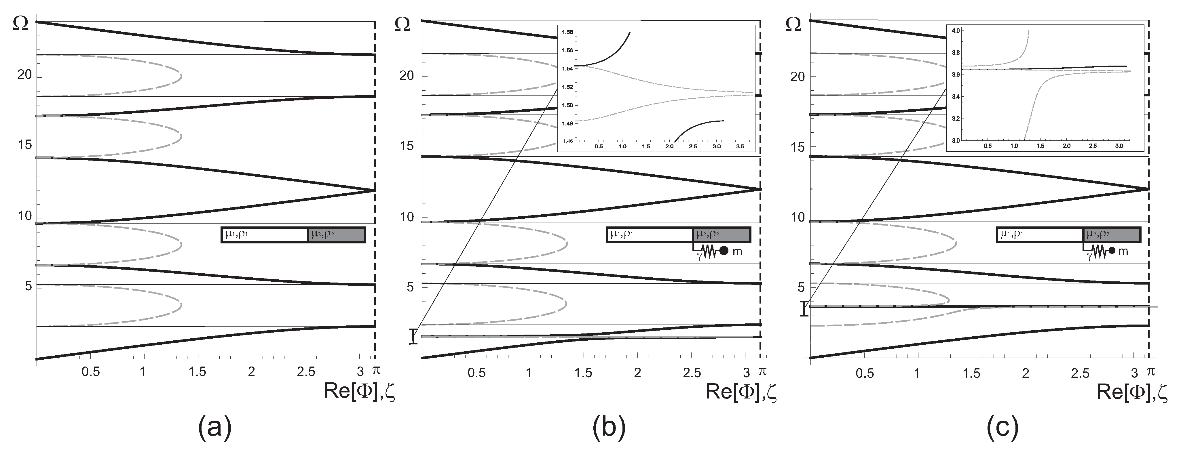
In Figure 6, dispersion diagrams are shown for the simple bi-layered laminate (part (a)) and for the cases where two different oscillators are included in the unit cell (parts (b) and (c)). For the laminate, ${\xi }_c=0.22$ and ${\eta }_c=0.5$, whereas the two oscillators are characterised by the impedance and frequency ratios ${\xi }_m=8.71$, ${\eta }_m=1.260$ (case (b)) and ${\xi }_m=8.71$, ${\eta }_m=0.525$ (case (c)). It is evident that the introduction of the oscillator induces a localised effect in the neighbourhood of its characteristic frequency ${\omega }_m$ without altering the dispersion properties of the system in the rest of the frequency spectrum. In particular, it creates a thin stop band if ${\omega }_m$ is in a pass band of the laminate (see case (b) in Figure 6) and a pass band if ${\omega }_m$ is in a stop band of the laminate (see case (c) in Figure 6).

Note that, for $\Omega =\delta /{\eta }_m$, the decay exponent $\zeta \to \infty$, as shown in the insets of Figure 6b,c, annihilating a propagating wave at this particular frequency.

Note also the slope inversion effect of the dispersion curves. In fact, for the simple laminate, different branches alternate the slope (namely, the group velocity) from positive to negative and vice versa. The introduction of the discrete resonator generates two consecutive curves with group velocity of the same sign.

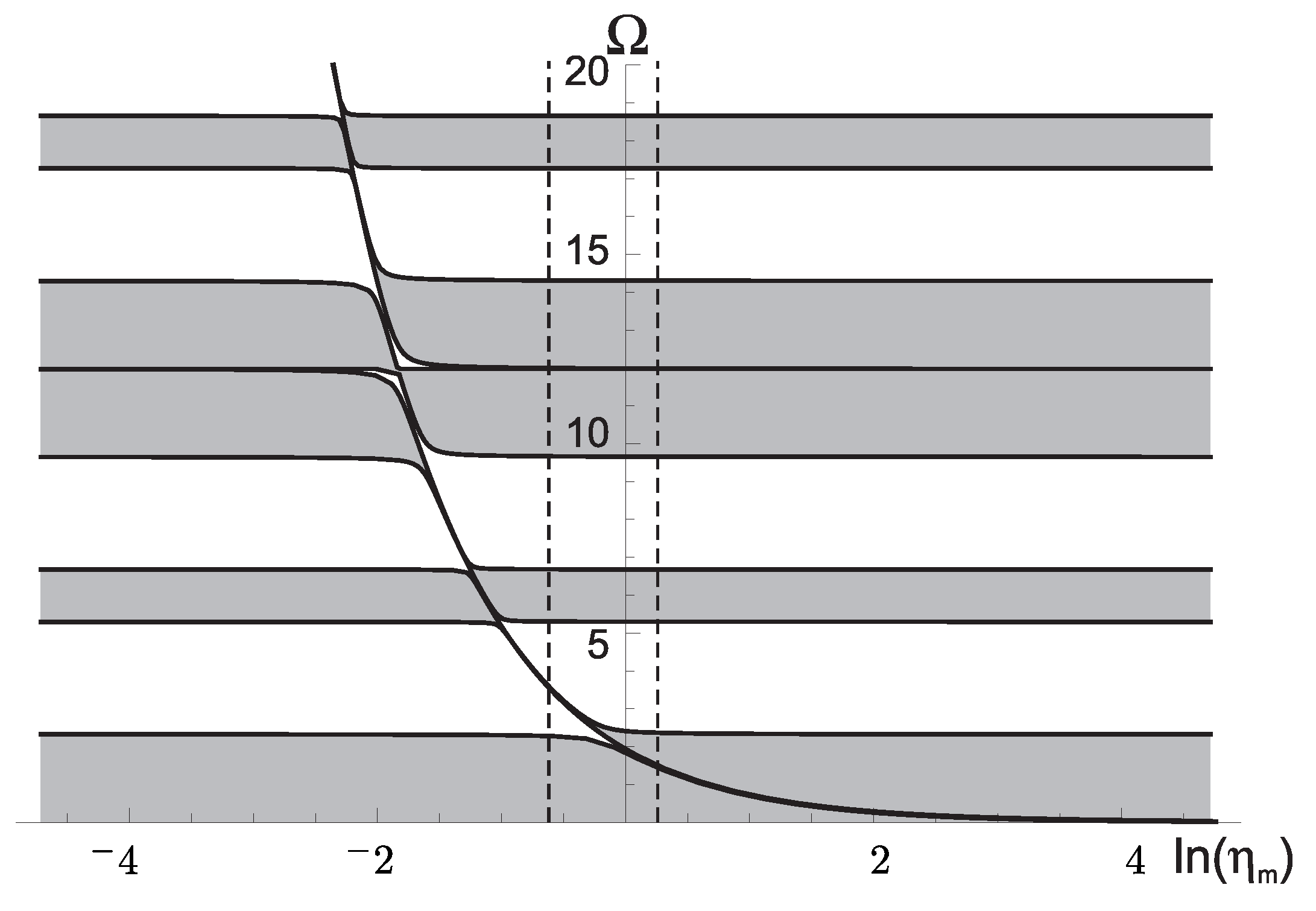
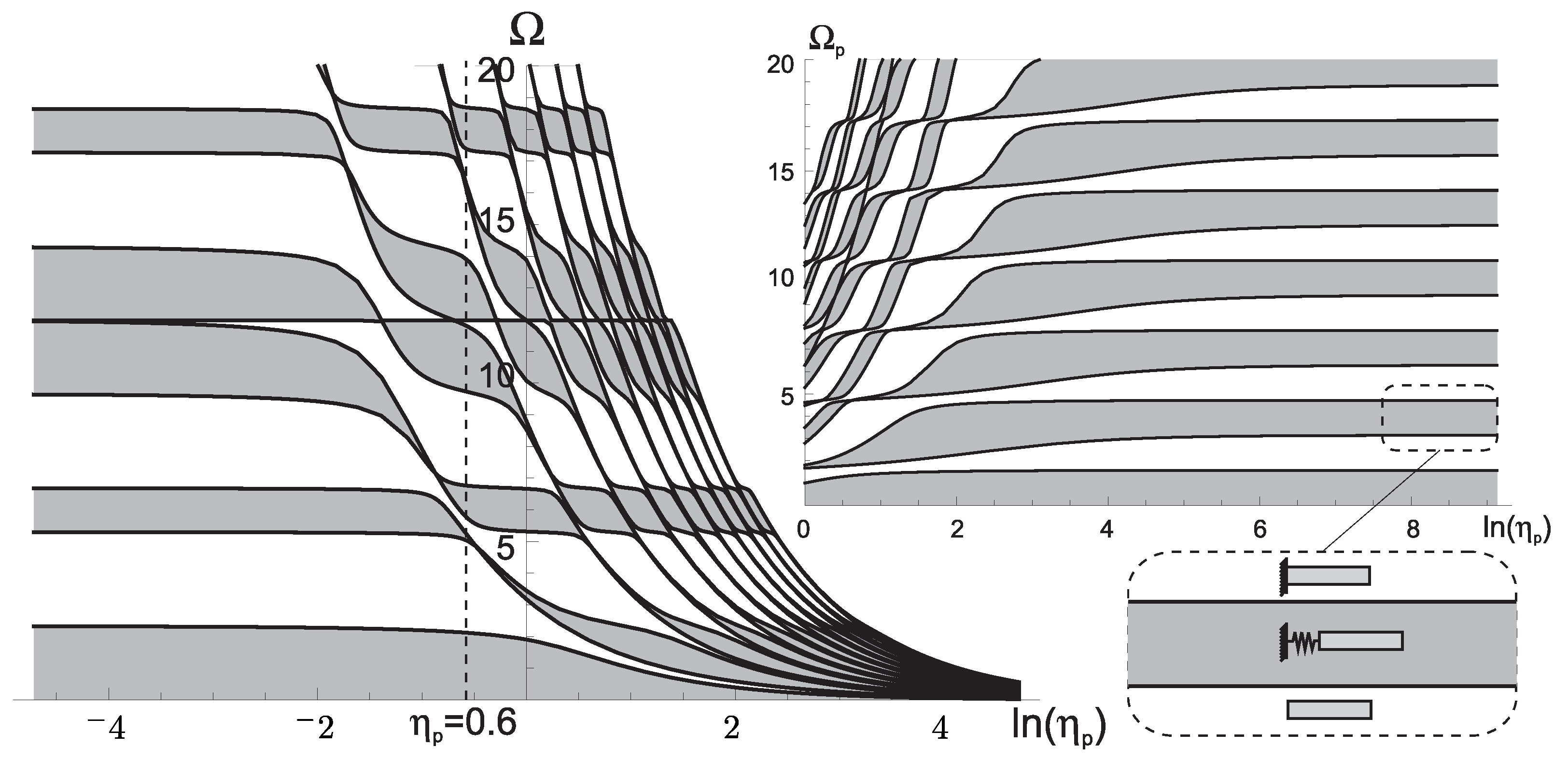
In Figure 7, the distribution of the bands are given as a function of the ratio ${\eta }_m$ for ${\xi }_c=0.22$, ${\eta }_c=0.5$ and ${\xi }_m=8.71$. It is shown that in the whole range of ${\eta }_m$ considered, the perturbation induced by the oscillator is always localised closed to the characteristic frequency of the oscillator and slightly larger when ${\omega }_m$ approaches the upper or lower limit frequencies of one band. Note also that in the limit ${\xi }_m\to \infty$, Equation (20) tends to the dispersion Equation (16), except in the neighbourhood of the singularity point $({\eta }_m/\delta )\Omega =1$, where a competing effect between ${\xi }_m$ and $1-{({\eta }_m/\delta )}^2{\Omega }^2$ arises.

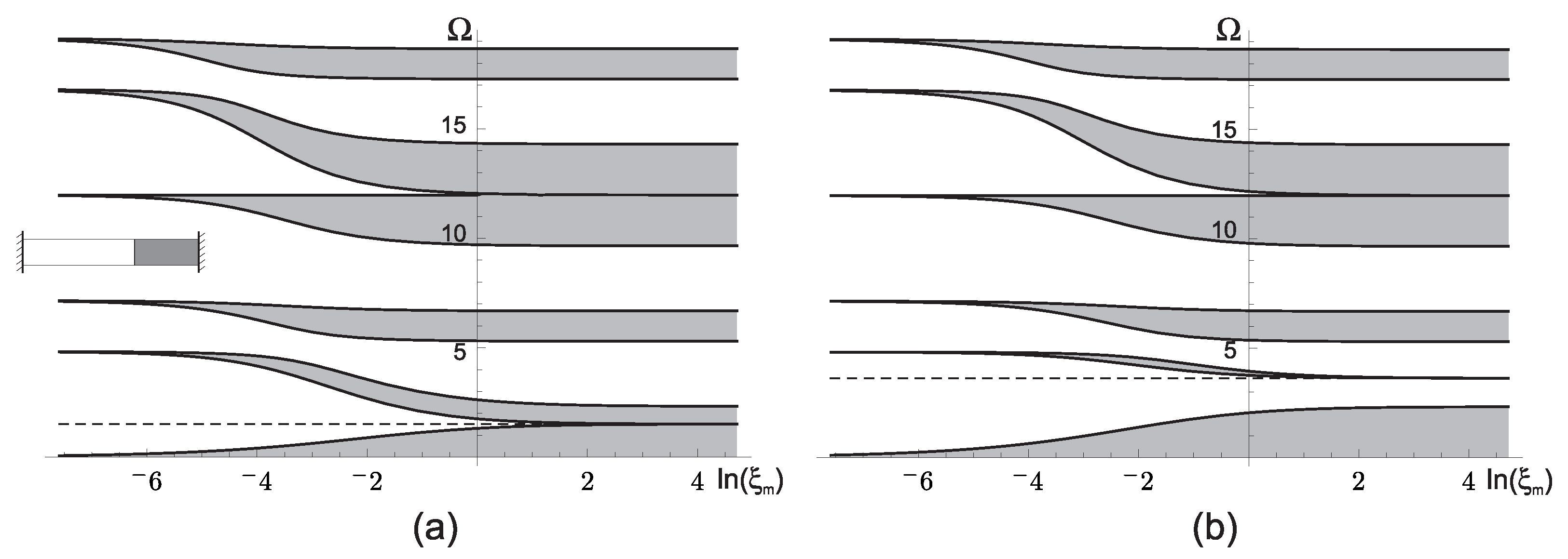
In contrast, in Figure 8 it is shown that the impedance ratio ${\xi }_m$ governs the transition between a discrete–continuous-like behaviour, for large negative values of $ln\left({\xi }_m\right)$, and a continuous-like one for large positive values of $ln\left({\xi }_m\right)$. In particular, when the elastic impedance of the oscillator tends to infinity, namely for $ln{\xi }_m\to -\infty$, the leading order term in Equation (20) is:

$$\left[\left(1+{\xi }_c\right)sin{\varphi }_{+}+\left(1-{\xi }_c\right)sin{\varphi }_{-}\right]\frac{\frac{{\eta }_m}{\delta }\Omega }{1-{\left(\frac{{\eta }_m}{\delta }\right)}^2{\Omega }^2}.$$

(21)

In this case, each unit cell behaves as the clamped two-phase system of finite size, sketched in the inset in Figure 8a, whose discrete eigenfrequencies are the roots of the term within square brackets in Equation (21). These values correspond to the central frequencies of the tiny bands for large negative $ln{\eta }_m$. Note the presence of an infinite number of bands due to the continuous phases, but band intervals of increasingly negligible size, as a result of the discrete oscillator.

When the elastic impedance of the oscillator is relatively small, namely for large $ln\left({\xi }_m\right)$, the ratio $1/{\xi }_m$ makes the contribution of the term (21) in Equation (20) small, except in the vicinity of the characteristic frequency $\Omega =\delta /{\eta }_m$. In such a case, the continuous-like behaviour is similar to the one in Figure 7. The transition between the different behaviours described above is roughly in the interval $-5\le ln\left(\xi \right)\le 0$, and the interaction between the continuous and the discrete phases can be attributed to the expression (21) divided by $4{\xi }_m$ in Equation (20).

The width of the stop band generated by the oscillator with ${\eta }_m=1.26$ (Figure 8a) increases monotonically as ${\xi }_m$ decreases, while the propagating band created by the oscillator with ${\eta }_m=0.525$, namely the first optical pass band, has maximum bandwidth in the transition zone, for $-3\le ln\left({\xi }_m\right)\le 0$ (Figure 8b).

3.2.2. Continuous Phase in Parallel

We investigate now the effect of a continuous phase arranged in parallel at the interface of the bi-layer laminate system, as indicated in the inset of Figure 9a. The transfer matrix ${\mathbf{M}}_T$ of the unit cell can be built as for the case of a single oscillator in parallel with the difference that ${\mathbf{M}}_{\chi }$ is now in the form of (5). We introduce the additional characteristic frequency and impedance ratios as ${\eta }_p={\omega }_1/{\omega }_3$ and ${\xi }_p=q_1/q_3$, respectively, where ${\omega }_3=\sqrt{{\mu }_3/{\rho }_3}/d_3$ and $q_3=d_3\sqrt{{\mu }_3{\rho }_3}$ refer to the phase in parallel, as shown in the inset of Figure 9a.

The dispersion relation takes the form:

$$\begin{array}{ccc}\hfill cos\varphi & =& \frac{1}{4}\left[\frac{{(1+{\xi }_c)}^2}{{\xi }_c}cos{\varphi }_{+}-\frac{{(1-{\xi }_c)}^2}{{\xi }_c}cos{\varphi }_{-}\right]+\hfill \\ & & -\frac{1}{4{\xi }_p}\left[(1+{\xi }_c)sin{\varphi }_{+}+(1-{\xi }_c)sin{\varphi }_{-}\right]tan\frac{{\eta }_3}{\delta }\Omega .\hfill \end{array}$$

(22)

The terms within the first square bracket on the right-hand side of Equation (22) correspond to the right-hand side of the dispersion Equation (11), describing the effect of the two continuous phases in series. The comparative analysis between the dispersion Equations (20) and (22) shows that they only differ in the terms including the singularity, namely:

$$\frac{\frac{{\eta }_m}{\delta }\Omega }{1-{\left(\frac{{\eta }_m}{\delta }\right)}^2{\Omega }^2}\mathrm{and}tan\frac{{\eta }_p}{\delta }\Omega .$$

(23)

The two above expressions have simple poles at the corresponding characteristic frequencies, a single frequency $\Omega =\delta /{\eta }_m$ for the discrete case (we do not consider the negative frequency $\Omega =-\delta /{\eta }_m$) and the multiple frequencies:

$$\tilde{\Omega }\simeq \frac{1+2n}{2}\pi \frac{\delta }{{\eta }_p},n\in {\mathcal{N}}_0,$$

(24)

for the continuous one.

Similar to the dispersion equation for the discrete resonator, the second term within square brackets on the right-hand side of Equation (22) reflects the presence of the continuous phase in parallel. The comparative analysis between the dispersion diagrams of Figure 6 and Figure 9a reveals that the presence of the continuous phase in parallel introduces multiple flat bands in the vicinity of the normalised eigenfrequencies:

$$\tilde{\Omega }\simeq \frac{1+2n}{2}\pi \frac{\delta }{{\eta }_p},n\in {\mathcal{N}}_0,$$

(25)

when ${\xi }_p$ is sufficiently large. These are the eigenfrequencies of the finite system indicated in the top right inset in Figure 9b, where the single continuous phase in parallel has clamped and free boundary conditions.

This effect is similar to the case of Section 3.2.1: for the discrete oscillator, a single additional band is created, whereas for the continuous phase, multiple bands are generated in the neighbourhood of the eigenfrequencies reported in (25), the constant frequency interval between eigenfrequencies being $\Delta \tilde{\Omega }=\pi \delta /{\eta }_p$.

Indeed, this is particularly evident by looking at the band distributions as a function of the characteristic frequency ratios ${\eta }_m$ in Figure 7 and ${\eta }_p$ in Figure 10, which reveal that the bands created by the bi-layered laminate (which can be recognised looking at the limit $ln\left({\eta }_m\right),ln\left({\eta }_p\right)\to -\infty$, respectively) are perturbed in correspondence of the eigenfrequencies of the system arranged in parallel: a single eigenfrequency for the discrete oscillator, multiple ones for the continuous phase.

It is also interesting to focus the attention on the optical band corresponding to the the continuous phases in parallel for large values of the characteristic frequency ratio ${\eta }_p$; to this purpose, on the right of Figure 10, the band distribution is also given in terms of the normalised frequency ${\Omega }_p=\omega /{\omega }_p$. We note that the pass bands are bounded by frequencies, which can be determined analytically from simple finite mechanical models regarding the additional phase $\chi$ in parallel. The lower bound corresponds to the system with two free ends and the upper bound to the system with clamped and free boundary conditions as detailed in the inset of Figure 10. Clearly, the free, clamped or elastic boundary condition is determined by the dynamic interaction between the bi-layer (arranged in series) and the resonator (arranged in parallel).

3.3. Single Oscillator in Series

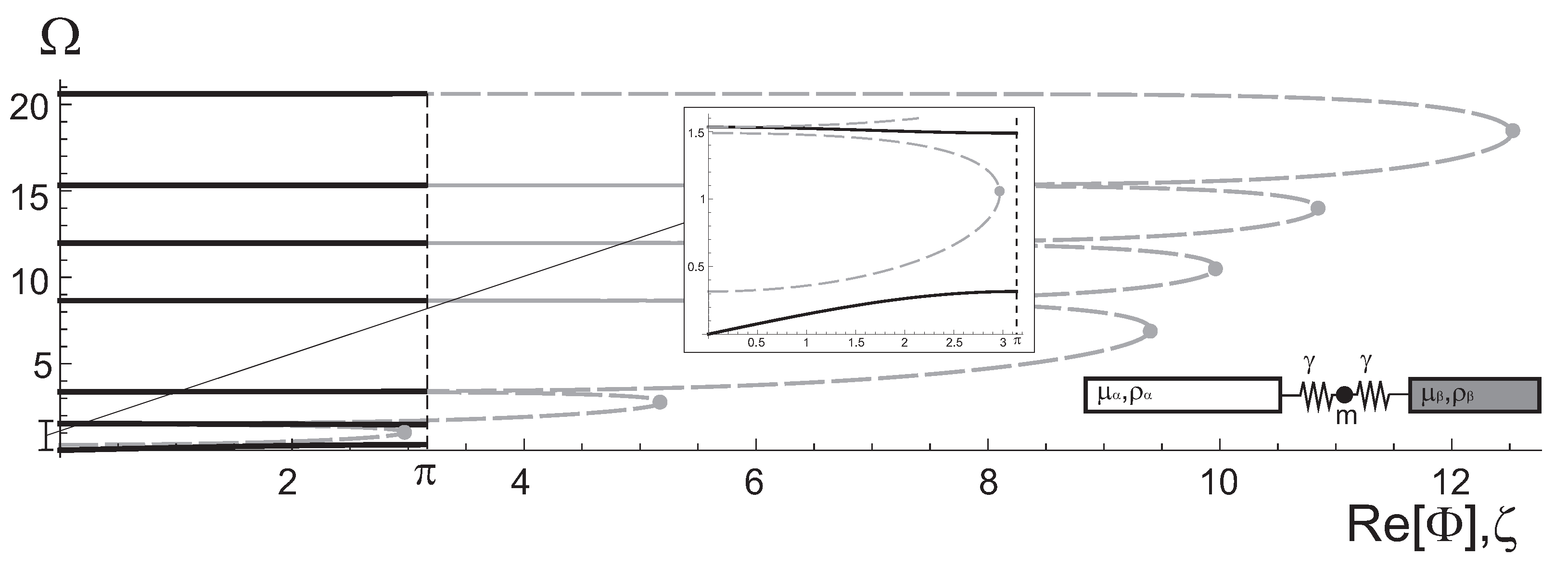
We consider a discrete oscillator arranged in series between the two continuous phases as in the inset of Figure 11. The transfer matrix of the unit cell can be obtained by direct multiplication of the transfer matrix of the single phases as in Equation (8), namely ${\mathbf{M}}_S={\mathbf{M}}_{\beta }{\mathbf{M}}_{\chi }{\mathbf{M}}_{\alpha }$, where ${\mathbf{M}}_{\alpha }$ and ${\mathbf{M}}_{\beta }$ are in the the form of (5) and ${\mathbf{M}}_{\chi }$ in the form of (6). The dispersion relation is:

$$\begin{array}{ccc}\hfill cos\varphi & =& \frac{1}{4}\left[\frac{{(1+{\xi }_c)}^2}{{\xi }_c}cos{\varphi }_{+}-\frac{{(1-{\xi }_c)}^2}{{\xi }_c}cos{\varphi }_{-}\right]\left[1-2{\left(\frac{{\eta }_m}{\delta }\right)}^2{\Omega }^2\right]+\hfill \\ & & -\frac{1}{4{\xi }_m}[(1+{\xi }_c)sin{\varphi }_{+}+(1-{\xi }_c)sin{\varphi }_{-}]\frac{{\eta }_m}{\delta }\Omega +\hfill \\ \hfill & & -\frac{{\xi }_m}{{\xi }_c}[(1+{\xi }_c)sin{\varphi }_{+}-(1-{\xi }_c)sin{\varphi }_{-}]\frac{{\eta }_m}{\delta }\Omega \left[1-{\left(\frac{{\eta }_m}{\delta }\right)}^2{\Omega }^2\right].\hfill \end{array}$$

(26)

In this case, the characteristic frequency of the discrete oscillator is ${\omega }_m=\sqrt{2\gamma /m}$ and its elastic impedance is $q_m=\sqrt{2\gamma m}$; they define the frequency ${\eta }_m={\omega }_1/{\omega }_m$ and impedance ${\xi }_m=q_1/q_m$ ratios as previously.

In Figure 11, the dispersion diagram and the decay exponent are shown for the bi-layered laminate with the discrete oscillator arranged in series.

The presence of the discrete oscillator drastically alters the dispersion properties in the whole frequency range: as a consequence of its introduction, narrower and narrower pass bands are obtained at increasing frequency; on the other hand, the central frequency of each band is determined by the continuous phases. By inspection of Equation (26), it is clear that the polynomial terms in $({\eta }_m/\delta )\Omega$, associated with the discrete oscillator, change the dispersive behaviour of the micro-structured system. Polynomial terms in $({\eta }_m/\delta )\Omega$ increase in magnitude with the frequency and generate wider and wider stop bands, where $cos\varphi >1$. Such a polynomial dependence induces larger attenuation, as evidenced by the decay exponent $\xi$ in Figure 11, which has increasing maximum values passing from one stop band to the next one.

In turn, the frequency position of the narrower and narrower pass bands are determined by the continuous phases, associated with the trigonometric terms in ${\varphi }_{+}$ and ${\varphi }_{-}$, which make the absolute value of the right-hand side of Equation (26) less than 1.

The continuous nature of the micro-structured system is also linked to the fact that the system is not a low-pass filter and, in principle, it can support waves without a frequency upper limit.

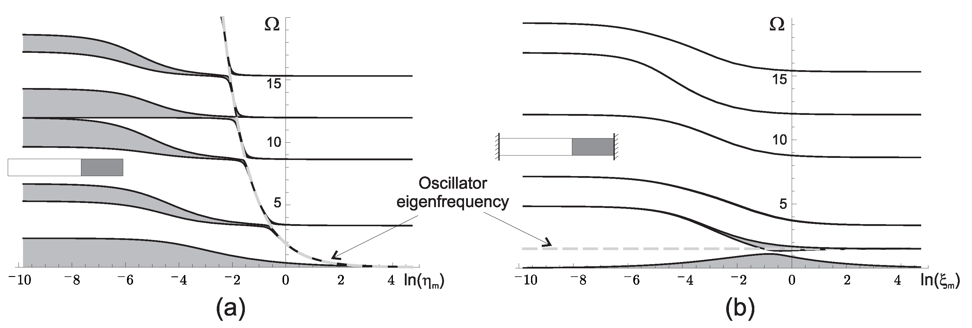
The distributions of the bands in term of the eigenfrequency ratio ${\eta }_m$ and the impedance ratio ${\xi }_m$ are detailed in Figure 12a,b, respectively. The oscillator eigenfrequency $\Omega =\delta /{\eta }_m$, indicated in dashed grey line, is a threshold between two different behaviours: below this critical eigenfrequency, the system has a “continuous” dispersive character, where the sizes of pass and stop bands are in general of the same order. In particular, in the limit ${\eta }_m\to 0$, the dispersion Equation (26) reduces to (16) associated with the laminate described in Section 3.

Above this threshold value, the system has the “discrete-continuous” character described in Figure 11, with highly localised pass bands over the all frequency axis that are positioned accordingly to the continuous phases.

Finally, it is interesting to look at the limiting cases: for ${\xi }_m\to 0$ each cell behaves as the double-clamped bilayer, already described in Section 3.2.1 and indicated in the insert of Figure 12b, whose eigenfrequencies are the zeros of (21). For ${\eta }_m,{\xi }_m\to \infty$, each unit cell behaves like a finite continuous bilayer with stress free boundary conditions whose eigenfrequency are the solutions in term of $\Omega$ of the equation:

$$\left[(1+{\xi }_c)sin{\varphi }_{+}-(1-{\xi }_c)sin{\varphi }_{-}\right]\Omega =0.$$

(27)

Note that in the case ${\xi }_m\to \infty$, there is an additional eigenfrequency corresponding to $\Omega =\delta /{\eta }_m$.

For the purpose of completeness, we list in Appendix A the transfer matrices of the systems described above.

4. Energy Distribution

In this section, we detail the energy distribution between different units for some configurations in series and in parallel described previously.

We compute the total energy $e\left(t\right)$ starting from the balance of mechanical energy (or theorem of power expended):

$$\frac{d}{dt}K\left(t\right)+P_{int}\left(t\right)=P_{ext}\left(t\right),$$

(28)

where $K\left(t\right)$ is the kinetic energy, $P_{int}\left(t\right)$ the stress-power and $P_{ext}\left(t\right)$ the external mechanical power. The balance Equation (28) can be applied to every part of the considered system, in particular, to the single phases or the unit cell. Since a conservative mechanical system is considered, the external mechanical power $P_{ext}\left(t\right)$ can be expressed by virtue of the rate of external potential energy $U_{ext}\left(t\right)$, namely $P_{ext}\left(t\right)=-d{U}_{ext}\left(t\right)/dt$, and the stress power $P_{int}\left(t\right)$ can be expressed by virtue of the rate of internal potential energy (or total strain energy) $U_{int}\left(t\right)$, namely $P_{int}\left(t\right)=d{U}_{int}\left(t\right)/dt$. By means of these assumptions, the balance of mechanical energy implies that the total energy $e\left(t\right)$, sum of the potential energy $U\left(t\right)=U_{int}\left(t\right)+U_{ext}\left(t\right)$ and the kinetic energy $K\left(t\right)$ is conserved (constant) during a dynamical process:

$$e\left(t\right)=K\left(t\right)+U\left(t\right)=\mathrm{const}.$$

(29)

Then, in a continuous phase $\alpha$, the total energy $E_{\alpha }$ is obtained averaging $e\left(t\right)$ over a period $2\pi /\omega$ as:

$$E_{\alpha }=\frac{1}{2}{\mu }_{\alpha }{k}_{\alpha }^2(A_{\alpha }{\overline{A}}_{\alpha }+B_{\alpha }{\overline{B}}_{\alpha })d_{\alpha },$$

(30)

where $A_{\alpha }$ and $B_{\alpha }$ are the complex amplitudes of the displacement $U_{\alpha }\left(x\right)$, as in Equation (2), and ${\overline{A}}_{\alpha }$ and ${\overline{B}}_{\alpha }$ their complex conjugates. The complex amplitudes may be computed from the transfer matrices of the single phases or the unit cells; in particular, referring for simplicity to a single continuous phase $\alpha$ disposed between $x_0$ and $x_1=x_0+d_{\alpha }$:

$${\mathbf{v}}_{\alpha }\left(x_1\right)={\mathbf{M}}_{\alpha }{\mathbf{v}}_{\alpha }\left(x_0\right)=e^{\pm i{\varphi }_{\alpha }}{\mathbf{v}}_{\alpha }\left(x_0\right),$$

(31)

where ${\mathbf{v}}_{\alpha }\left(x\right)={\left[U_{\alpha }\left(x\right){\tau }_{\alpha }\left(x\right)\right]}^T$. Therefore, the transfer matrix ${\mathbf{M}}_{\alpha }$ has eigenvalues $e^{\pm i{\varphi }_{\alpha }}$ corresponding to propagation towards the positive and negative $x$-direction, respectively, and eigenvectors ${\tilde{\mathbf{v}}}_{\alpha }^{\pm }$. Then, following the representation (2):

$${\tilde{\mathbf{v}}}_{\alpha }^{\pm }={\mathbf{H}}_{\alpha }{\mathbf{a}}_{\alpha }^{\pm },\mathrm{with}{\mathbf{H}}_{\alpha }=\left[\begin{array}{cc}{e}^{i{k}_{\alpha }{x}_0}& e^{-i{k}_{\alpha }{x}_0}\\ i{k}_{\alpha }{\mu }_{\alpha }{e}^{i{k}_{\alpha }{x}_0}& -i{k}_{\alpha }{\mu }_{\alpha }{e}^{-i{k}_{\alpha }{x}_0}\end{array}\right],{\mathbf{a}}_{\alpha }^{\pm }=\left\{\begin{array}{c}{A}_{\alpha }^{\pm }\\ B_{\alpha }^{\pm }\end{array}\right\}.$$

(32)

Relation (32) can be inverted to obtain the two sets of complex amplitudes ${\mathbf{a}}_{\alpha }^{+}$ and ${\mathbf{a}}_{\alpha }^{-}$.

The energy $E_{{\chi }_d}$ of the single oscillator arranged in parallel can be expressed in term of the amplitudes of the continuous phase 1 of Figure 13, identified with the label $\alpha$:

$$E_{{\chi }_d}=\frac{1}{2}\frac{\gamma m{\omega }^2(\gamma +m{\omega }^2)}{{(\gamma -m{\omega }^2)}^2}\left[\frac{A_{\alpha }{\overline{A}}_{\alpha }+B_{\alpha }{\overline{B}}_{\alpha }}{2}+\mathcal{R}e\left(A_{\alpha }{\overline{B}}_{\alpha }{e}^{i2{\varphi }_{\alpha }}\right)\right].$$

(33)

The energy $E_{{\chi }_c}$ of the continuous phase arranged in parallel can be computed by implementing the relevant transfer matrix as given in Equation (10). Finally, the energy $E_{S_d}$ of the single oscillator arranged in series is given by:

$$\begin{array}{ccc}\hfill E_{S_d}& =& \frac{1}{2}\frac{\gamma }{{(2\gamma -m{\omega }^2)}^2}[\frac{2{\gamma }^2-\gamma m{\omega }^2+m^2{\omega }^4}{2}(A_d{\overline{A}}_d+B_d{\overline{B}}_d)-\hfill \\ & & -(2{\gamma }^2-3\gamma m{\omega }^2)\mathcal{R}e\left(A_d{\overline{B}}_d\right)].\hfill \end{array}$$

(34)

where $A_d$ and $B_d$ are the complex displacement amplitudes.

In Figure 13, Figure 14 and Figure 15, we present the distribution of the energies within the phases as a function of the frequency $\omega$ for the mechanical systems described in the previous section, where the additional phase is arranged in parallel and in series. The energies are normalised by the total energy stored in the unit cells and are presented with dashed lines for the bi-phase system and with continuous lines for the different tri-phase systems. We note that the energies corresponding to waves propagating in opposite direction are coincident in the propagating bands and distinct in the stop bands. In the last case, the upper curves correspond to the propagation direction.

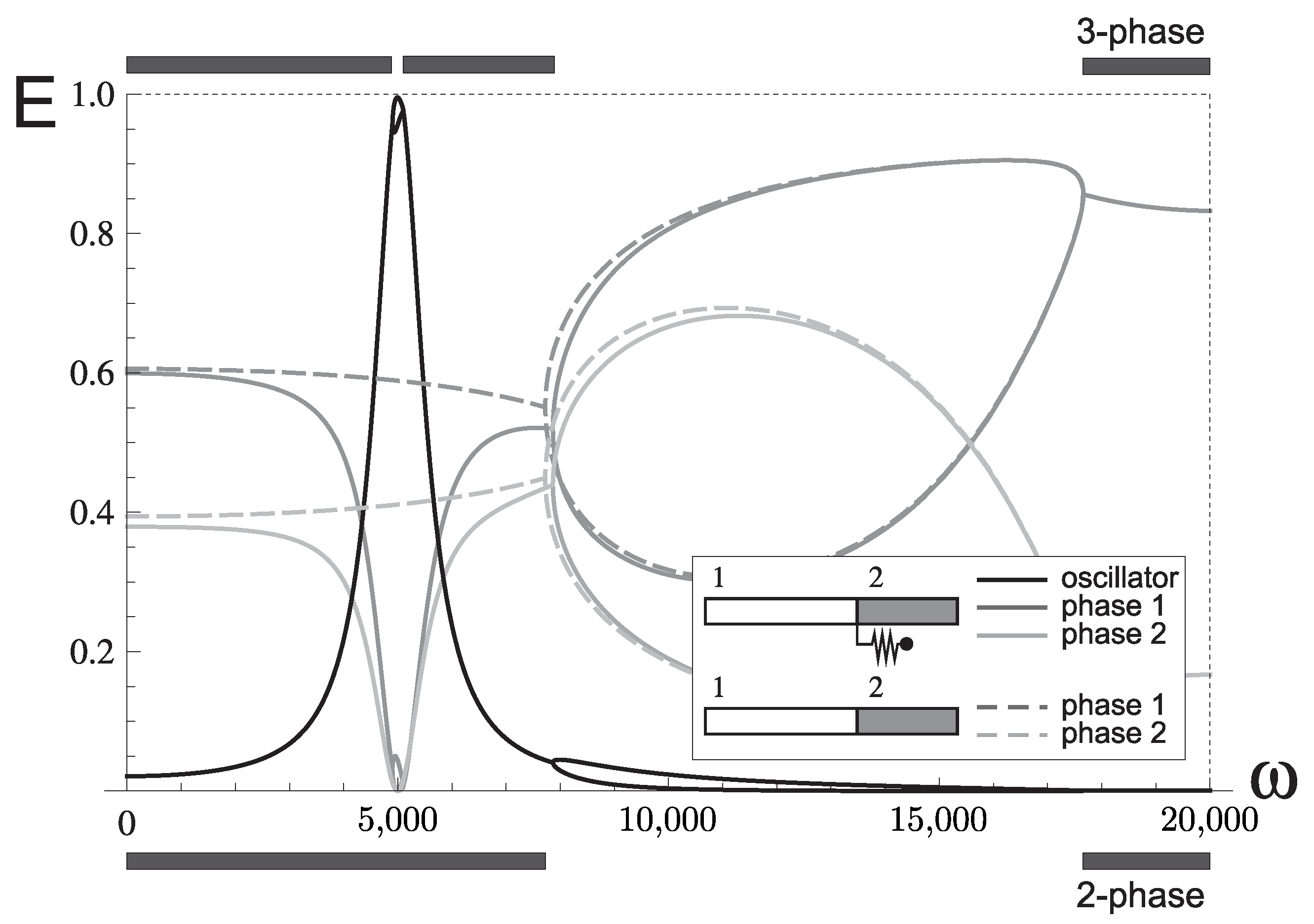
In Figure 13, we present the effect of the discrete oscillator arranged in parallel. The comparative analysis with the two-phase system shows that, in correspondence of the characteristic frequency ${\omega }_m$, the energy is almost entirely localised in the discrete oscillator, whereas, departing from this frequency, the behaviour tends to be practically coincident to the bi-laminate. This is fully consistent with the outcomes of Figure 7.

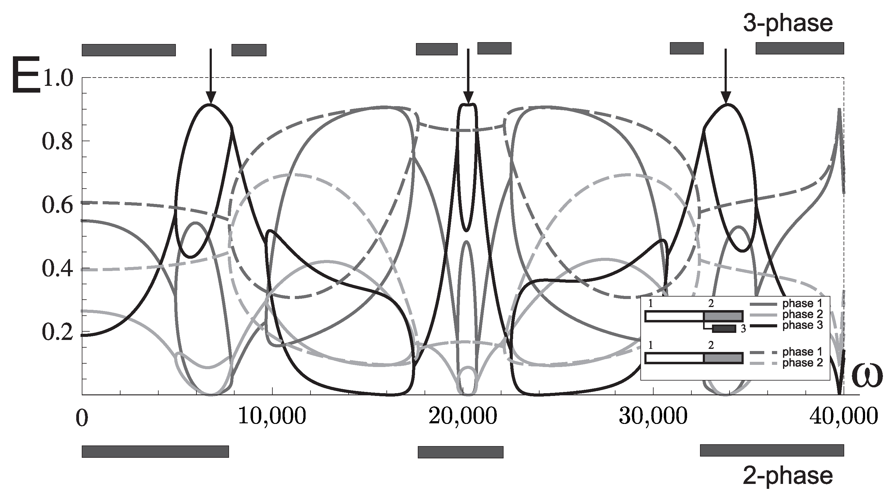
The effects of the continuous phase arranged in parallel are shown in Figure 14. It can be seen that the continuous phase arranged in parallel localises most of the energy in correspondence of its eigenfrequencies (indicated with three arrows), even if the amount of stored energy does not reach the same peak as for the discrete oscillator.

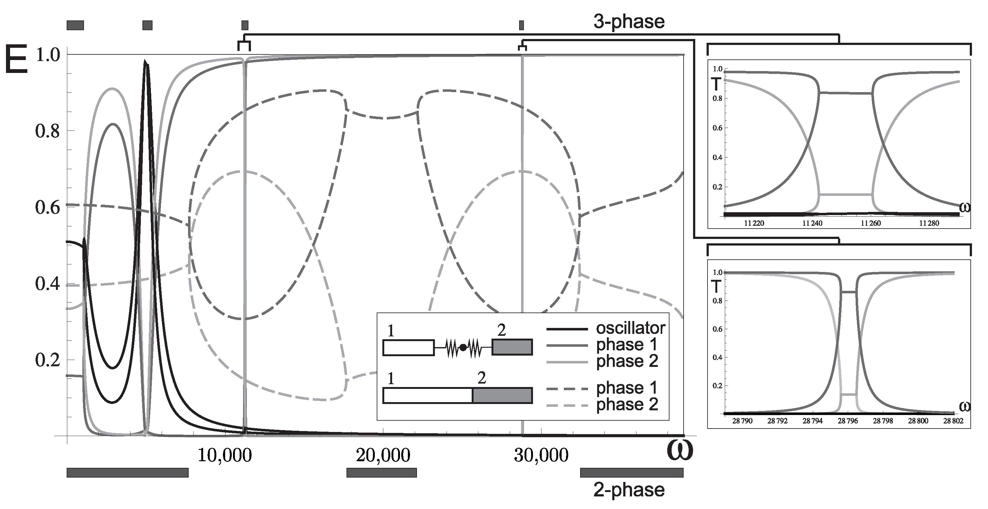
Finally, in Figure 15, the effect of the discrete oscillator arranged in series is shown. As for the dispersion diagram, the introduction of the discrete phase radically changes the dynamic behaviour of the continuous phases. It is noted that the energy is concentrated in the oscillator in correspondence of its characteristic frequency, but not in the thin pass band opened at higher frequencies. Furthermore, the high energy concentration in the phases in the higher frequency stop bands is an indication of the high level of attenuation, as shown in Figure 11.

5. Conclusions

Filtering properties of systems having a continuous and discrete character and arranged in series and parallel have been considered. The analysis has been done by implementing a transfer matrix approach; the analytical model simplifies the identification of the contributions of mechanical properties, phase character and arrangement.

The model has been given for out-of-plane shear waves, which are governed by Helmholtz type equations of motion, so that the results can be easily extended to other physical applications governed by the same type of equation, such as longitudinal or torsional waves in a rod (for sufficiently low frequencies), as well as acoustics and optics.

Several properties have been detected, which can be implemented in different applications.

In the laminate system, it has been shown that dispersion is induced by the elastic impedance contrast, namely for ${\xi }_c\ne 1$, whereas the frequency contrast does not necessarily introduce any dispersion.

For oscillators arranged in parallel, localised effects are obtained, where most of the energy is confined in the resonators. This effect is implemented when tuned mass dampers are added to a structure in order to damp dangerous vibrations. The simple model developed in this work shows that energy localisation is higher for the discrete oscillator, but the continuous one gives the possibility to obtain this effect at multiple frequencies. The analysis also shows that this type of localisation, where the dispersive behaviour of the system in series is strongly perturbed only in the neighbourhood of the resonance frequencies of the oscillator, is retrieved when the elastic impedance of the resonator is sufficiently small.

If systems having discrete and continuous character are arranged in series, the dispersion properties drastically change, combining the effect of creating tiny pass/stop bands typical of discrete systems with the frequency periodicity or quasi-periodicity induced by the continuous ones. Such behaviour, addressed as continuous–discrete like, can have direct application in delay-line components, where there is the necessity to slow down waves and energy propagation, which is associated with the group velocity (the slope of the dispersion curves), with a small amount of reflection.

A similar continuous discrete-like behaviour is obtained for a phase arranged in parallel, when the elastic impedance of the resonator is sufficiently high. In both cases, it is possible to predict the central frequencies of the tiny pass bands by evaluating the eigenfrequencies of an isolated single unit cell with ad hoc boundary conditions. These types of systems can be implemented in order to propagate selected frequencies at a constant interval. For the systems in parallel, this behaviour is obtained when the elastic impedance of the resonator is sufficiently high, while for the system in series, this is obtained when the frequency of the incoming wave is above the resonance frequency of the discrete oscillator, a condition that is reasonably easier to reach in technological applications.

The transition regions between the continuous-discrete and the continuous-like behaviours can be explored to enlarge the frequency intervals, where the localisation induced by the resonators is still effective.

The results presented in this work can find applications that range from the control of mechanical vibrations in large scale structures, such as slender bridges, to frequency filtering in Micro and Nano Electro-Mechanical Systems.

References

- Elmore, W.C.; Heald, M.A. Physics of Waves; McGraw-Hill: New York, NY, USA, 1969. [Google Scholar]
- Mason, W.P. Electromechanical Transducers and Wave Filters; Van Nostrand: New York, NY, USA, 1942. [Google Scholar]
- Brillouin, L. Wave Propagation in Periodic Structures; Dover: New York, NY, USA, 1946. [Google Scholar]
- Laude, V. Phononic Crystals: Artificial Crystals for Sonic, Acoustic, and Elastic Waves; De Gruyter: Germany, Berlin, 2020. [Google Scholar]
- Voiculescu, I.; Nordin, A.N. Acoustic wave based MEMS devices for biosensing applications. Biosens. Bioelectron. 2012, 33, 1–9. [Google Scholar] [CrossRef] [PubMed]
- Collin, R.E. Foundations for Microwave Engineering, 2nd ed.; McGraw-Hill: London, UK, 2000. [Google Scholar]
- Yousefian, M.; Hosseini, S.J.; Dahmardeh, M. Compact broadband coaxial to rectangular waveguide transition. J. Electromagn. Waves Appl. 2019, 33, 1239–1247. [Google Scholar] [CrossRef]
- Ewing, M.W. Elastic Waves in Layered Media; McGraw-Hill: New York, NY, USA, 1957. [Google Scholar]
- Yeh, P. Optical Waves in Layered Media; Wiley-Interscience: Hoboken, NJ, USA, 2005. [Google Scholar]
- Cooper, A.J.; Crighton, D.G. Transmission of energy down periodically ribbed elastic structures under fluid loading: Spatial periodicity in the pass bands. Proc. R. Soc. Lond. A 1998, 454, 2893–2909. [Google Scholar] [CrossRef]
- Evans, D.V.; Porter, R. Penetration of flexural waves through a periodically constrained thin elastic plate in vacuo and floating on water. J. Eng. Math. 2007, 58, 317–337. [Google Scholar] [CrossRef]
- Haslinger, S.G.; Movchan, N.V.; Movchan, A.B.; McPhedran, R.C. Transmission, trapping and filtering of waves in periodically constrained elastic plates. Proc. R. Soc. Lond. A 2012, 468, 76–93. [Google Scholar] [CrossRef] [Green Version]
- Tie, B.; Tian, B.Y.; Aubry, D. Theoretical and numerical modeling of membrane and bending elastic wave propagation in honeycomb thin layers and sandwiches. J. Sound Vib. 2016, 382, 100–121. [Google Scholar] [CrossRef]
- Denke, P.M.; Eide, G.R.; Pickard, J. Matrix difference equation analysis of vibrating periodic structures. AIAA J. 1975, 13, 160–166. [Google Scholar] [CrossRef]
- Hsueh, W.J. Closed solutions of wave propagation in finite-periodic strings. Proc. R. Soc. Lond. A 2004, 460, 515–536. [Google Scholar] [CrossRef]
- Pereyra, P. Theory of finite periodic systems: The eigenfunctions symmetries. Ann. Physics 2017, 378, 264–279. [Google Scholar] [CrossRef] [Green Version]
- Wei, J.; Petyt, M. A method of analyzing finite periodic structures, part 1: Theory and examples. J. Sound Vib. 1997, 202, 555–569. [Google Scholar] [CrossRef]
- Wei, J.; Petyt, M. A method of analyzing finite periodic structures, part 2: Comparison with infinite periodic structure theory. J. Sound Vib. 1997, 202, 571–583. [Google Scholar] [CrossRef]
- Brun, M.; Giaccu, G.F.; Movchan, A.B.; Movchan, N.V. Asymptotics of eigenfrequencies in the dynamic response of elongated multi-structures. Proc. R. Soc. Lond. A 2012, 468, 378–394. [Google Scholar] [CrossRef]
- Carta, C.; Brun, M.; Movchan, A.B.; Boiko, T. Transmission and localisation in ordered and randomly-perturbed structured flexural systems. Int. J. Eng. Sci. 2016, 98, 126–152. [Google Scholar] [CrossRef]
- Carta, C.; Brun, M.; Movchan, A.B. Dynamic response and localisation in strongly damaged waveguides. Proc. R. Soc. Lond. A 2014, 470, 1–18. [Google Scholar] [CrossRef]
- Slepyan, L.I. Models and Phenomena in Fracture Mechanics; Springer: Berlin/Heidelberg, Germany, 2002. [Google Scholar]
- Marder, M.; Liu, X. Instability in lattice fracture. Phys. Rev. Lett. 1993, 71, 2417–2420. [Google Scholar] [CrossRef]
- Maradudin, A.; Weiss, G.H. On the Vibrations isedof a generalised diatomic lattice. J. Chem. Phys. 1958, 29, 631–634. [Google Scholar] [CrossRef]
- Maradudin, A.; Mazur, P.; Moentroll, E.W.; Weiss, G.H. Remarks on the vibrations of diatomic lattices. Rev. Mod. Phys. 1958, 30, 175–196. [Google Scholar] [CrossRef]
- Colquitt, D.J.; Jones, I.S.; Movchan, N.V.; Movchan, A.B.; McPhedran, R.C. Dynamic anisotropy and localisation in elastic lattice systems. Waves Random Complex Media 2012, 22, 143–159. [Google Scholar] [CrossRef]
- Martinsson, P.G.; Movchan, A.B. Vibrations of lattice structures and phononic band gaps. Quart. J. Mech. Appl. Math. 2003, 56, 45–64. [Google Scholar] [CrossRef]
- Graff, K.F. Wave Motion in Elastic Solids; Dover Publications: New York, NY, USA, 1975. [Google Scholar]
- Piccolroaz, A.; Movchan, A.B.; Cabras, L. Dispersion degeneracies and standing modes in flexural waves supported by Rayleigh beam structures. Int. J. Solids Struct. 2016, 109, 1–23. [Google Scholar] [CrossRef]
- Piccolroaz, A.; Movchan, A.B.; Cabras, L. Rotational inertia interface in a dynamic lattice of flexural beams. Int. J. Solids Struct. 2017, 112, 43–53. [Google Scholar] [CrossRef] [Green Version]
- Colombi, A.; Colquitt, D.; Roux, P.; Guenneau, S.; Craster, R.V. A seismic metamaterial: The resonant metawedge. Sci. Rep. 2016, 6, 27717. [Google Scholar] [CrossRef] [PubMed] [Green Version]
- Carta, G.; Colquitt, D.J.; Movchan, A.B.; Movchan, N.V.; Jones, I.S. One-way interfacial waves in a flexural plate with chiral double resonators. Proc. R. Soc. Lond. A 2020, 378, 20190350. [Google Scholar] [CrossRef] [PubMed] [Green Version]
- Carta, G.; Colquitt, D.J.; Movchan, A.B.; Movchan, N.V.; Jones, I.S. Chiral flexural waves in structured plates: Directional localisation and control. J. Mech. Phys. Solids 2020, 137, 103866. [Google Scholar] [CrossRef] [Green Version]
- Murakami, H. A mixture theory for wave propagation in angle-ply laminates, Part 1: Theory. J. Appl. Mech. 1985, 52, 331–337. [Google Scholar] [CrossRef]
- Nemat-Nasser, S.; Yamada, M. Harmonic waves in layered transversely isotropic composites. J. Sound Vib. 1981, 79, 161–170. [Google Scholar] [CrossRef]
- Pendry, J.B. Photonic band structures. J. Mod. Opt. 1994, 41, 209–229. [Google Scholar] [CrossRef]
- Nicorovici, N.A.; McPhedran, R.C.; Botten, L.C. Photonic band gaps for arrays of perfectly conducting cylinders. Phys. Rev. E 1995, 52, 1135–1145. [Google Scholar] [CrossRef]
- Parnell, W.J. Effective wave propagation in a pre-stresses nonlinear elastic composite bar. IMA J. Appl. Math. 2007, 72, 223–244. [Google Scholar] [CrossRef]
- Gei, M. Wave propagation in quasiperiodic structures: Stop/pass band distribution and effect of prestress. Int. J. Solids Struct. 2010, 47, 3067–3075. [Google Scholar] [CrossRef] [Green Version]
- Bigoni, D.; Movchan, A.B. Statics and dynamics of structural interfaces in elasticity. Int. J. Solids Struct. 2002, 39, 4843–4865. [Google Scholar] [CrossRef] [Green Version]
- Brun, M.; Guenneau, S.; Movchan, A.B.; Bigoni, D. Dynamics of structural interfaces: Filtering and focussing effects for elastic waves. J. Mech. Phys. Solids 2010, 58, 1212–1224. [Google Scholar] [CrossRef]
- Mead, D.J. A general theory of harmonic wave propagation in linear periodic systems with multiple coupling. J. Sound Vib. 1973, 27, 235–260. [Google Scholar] [CrossRef]
- Romeo, F.; Luongo, A. Invariants representation of propagation properties for bi-coupled periodic structures. J. Sound Vib. 2002, 257, 869–886. [Google Scholar] [CrossRef] [Green Version]
- Sen Gupta, G. Natural flexural waves and the normal modes of periodically-supported beams and plates. J. Sound Vib. 1970, 13, 89–101. [Google Scholar] [CrossRef]
- Carta, G.; Brun, M. Bloch-Floquet waves in flexural systems with continuous and discrete elements. Mech. Mater. 2015, 87, 11–26. [Google Scholar] [CrossRef]
- Movchan, A.B.; Slepyan, L.I. Band gap Green’s functions and localised oscillations. Proc. R. Soc. Lond. A 2007, 463, 2709–2727. [Google Scholar] [CrossRef]
- Kohn, W.; Krumhansl, J.A.; Lee, E.H. Variational methods for dispersion relations and elastic properties of composite materials. J. Appl. Mech. 1972, 39, 327–336. [Google Scholar] [CrossRef]
- Guo, W.; Yang, Z.; Feng, Q.; Dai, C.; Yang, J.; Lei, X. A new method for band gap analysis of periodic structures using virtual spring model and energy functional variational principle. Mech. Syst. Signal Process. 2022, 168, 108634. [Google Scholar] [CrossRef]
- Carta, G.; Giaccu, G.F.; Brun, M. A phononic band gap model for long bridges. The ‘Brabau’ bridge case. Eng. Struct. 2017, 140, 66–76. [Google Scholar] [CrossRef]
- McPhedran, R.C.; Movchan, A.B.; Movchan, N.V.; Brun, M.; Smith, M.J.A. ‘Parabolic’ trapped modes and steered Dirac cones in platonic crystals. Proc. R. Soc. Lond. A 2015, 471, 20140746. [Google Scholar] [CrossRef] [PubMed] [Green Version]
- Burlon, A.; Failla, G. Flexural wave propagation in locally-resonant beams with uncoupled/coupled bending-torsion beam-like resonators. Int. J. Mech. Sci. 2022, 215, 106925. [Google Scholar] [CrossRef]
- Gei, M.; Chen, Z.; Bosi, F.; Morini, L. Phononic canonical quasicrystalline waveguides. Appl. Phys. Lett. 2020, 116, 241903. [Google Scholar] [CrossRef]
- Morini, L.; Gei, M. Waves in one-dimensional quasicrystalline structures: Dynamical trace mapping, scaling and self-similarity of the spectrum. J. Mech. Phys. Solids 2018, 119, 83–103. [Google Scholar] [CrossRef] [Green Version]
- Bertoldi, K.; Bigoni, D.; Drugan, J.W. Structural interfaces in linear elasticity. Part I: Nonlocality and gradient approximations. J. Mech. Phys. Solids 2007, 55, 1–34. [Google Scholar] [CrossRef]
- Bertoldi, K.; Bigoni, D.; Drugan, J.W. Structural interfaces in linear elasticity. Part II: Effective properties and neutrality. J. Mech. Phys. Solids 2007, 55, 35–63. [Google Scholar] [CrossRef]
- Bertoldi, K.; Bigoni, D.; Drugan, J.W. A discrete-fibers model for bridged cracks and reinforced elliptical voids. J. Mech. Phys. Solids 2007, 55, 1016–1035. [Google Scholar] [CrossRef]
- Kozlov, V.; Maz’ya, V.; Movchan, A.B. Asymptotic Analysis of Fields in Multi-Structures; Oxford University Press: Oxford, UK, 1999. [Google Scholar]
- Morvaridi, M.; Carta, G.; Brun, M. Platonic crystal with low-frequency locally-resonant spiral structures: Wave trapping, transmission amplification, shielding and edge waves. J. Mech. Phys. Solids 2018, 121, 496–516. [Google Scholar] [CrossRef] [Green Version]
- Zeighami, F.; Palermo, A.; Marzani, A. Inertial amplified resonators for tunable metasurfaces. Meccanica 2019, 54, 253–265. [Google Scholar] [CrossRef]
- Lekner, J. Light in periodically stratified media. J. Opt. Soc. Am. A 1994, 11, 2892–2899. [Google Scholar] [CrossRef]
- Felbacq, D.; Guizal, B.; Zolla, F. Limit analysis of the diffraction of a plane wave by a one-dimensional periodic medium. J. Math. Phys. 1998, 39, 4604–4607. [Google Scholar] [CrossRef]
Figure 1.
Single units. (a) Continuous layer with shear modulus and density . ( b) Discrete unit with mass m and stiffness .
Figure 2.
Different arrangements of single units. (a) Two units in series. (b) Two units in parallel. (c) Three units: and are in series and is inserted in parallel at the interface between the others phases.
Figure 3.
Continuous laminate. Dispersion diagram and decay exponent for a two-layer continuous system. The Bloch parameter (continuous black lines) and the decay exponent (dashed grey lines) are given as a function of the angular frequency . The material and geometric parameters are: shear moduli, MPa, MPa; mass densities kg/m, kg/m; phase lengths m, m.
Figure 4.
Continuous laminate. Band distribution as a function of the characteristic frequency ratio . Normalised frequency is given for the impedance ratio . Filled areas indicate propagating bands. The dashed line corresponds to the case analysed in Figure 3. Blue circles highlight periodicity points.
Figure 5.
Continuous laminate. Band distribution as a function of the impedance ratio . Normalised frequency is given for the characteristic frequency ratio . In the upper right, a detail of the band distribution is given. On the bottom right, the same results are presented in term of . Filled area indicates propagating bands.
Figure 6.
Oscillator in parallel. Dispersion curves (continuous black lines) and decay exponent (dashed grey lines). Normalised frequency is given for and . (a) Bi-layered laminate. (b) Bi-layered laminate with oscillator, with , . (c) Bi-layered laminate with oscillator, with , .
Figure 7.
Oscillator in parallel. Band distribution as a function of the characteristic frequency ratio . Normalised frequency is given for , and . Dashed lines indicate the two cases analysed in Figure 8, and , respectively.
Figure 8.
Oscillator in parallel. Band distribution as a function of the impedance ratio . Normalised frequency is given for and . (a) , (b) . Dashed lines indicate the characteristic frequency of the oscillator.
Figure 9.
Continuous phase in parallel. Results are given for , . (a) Dispersion curves (continuous black lines) and decay exponent (dashed grey lines) for , . (b) Band distribution, where is given as a function of the impedance ratio ().
Figure 10.
Continuous phase in parallel. Band distribution as a function of the characteristic frequency ratio . The distribution of the bands are given in term of the normalised frequencies on the left and on the right. Impedance and frequency ratios are: , and . The dashed line at indicates the configuration of Figure 9a.
Figure 11.
Oscillator in series. Dispersion curves (continuous black lines) and decay exponent (dashed grey lines). Normalised frequency is given for , , and .
Figure 12.
Oscillator in series. Distribution of the propagation band frequency as a function of the ratios and . Results are given for and with in (a) and in (b). The grey dashed lines indicate the characteristic frequency of the oscillator.
Figure 13.
Energy distribution between different phases as a function of the radian frequency . Dashed lines correspond to the bi-layered system, while the continuous line corresponds to the bi-layered system with the oscillator disposed in parallel (indicated in black). Material and geometrical parameters are the same as Figure 6a,b. Pass band frequency intervals are indicated at the top and at the bottom of the plot.
Figure 14.
Energy distribution between different phases as a function of the radian frequency . Dashed lines correspond to the bi-layered system, while the continuous line corresponds to the bi-layered system with the continuous phase disposed in parallel (indicated in black). Results are given for , , and . Pass band frequency intervals are indicated at the top and at the bottom of the plot. Arrows indicate resonance frequencies of the phase arranged in parallel to the bi-layered system.
Figure 15.
Energy distribution between different phases as a function of the radian frequency . Dashed lines correspond to the bi-layered system, while the continuous line corresponds to the bi-layered system with the oscillator disposed in series (indicated in black). Details of the second and third pass-bands are given on the right. Material and geometrical parameters are the same as Figure 6a and Figure 11. Pass band frequency intervals are indicated at the top and at the bottom of the plot.
Publisher’s Note: MDPI stays neutral with regard to jurisdictional claims in published maps and institutional affiliations. |
© 2022 by the authors. Licensee MDPI, Basel, Switzerland. This article is an open access article distributed under the terms and conditions of the Creative Commons Attribution (CC BY) license (https://creativecommons.org/licenses/by/4.0/).
Share and Cite
MDPI and ACS Style
Sulis, S.; Rakhimzhanova, A.; Brun, M. Filtering Properties of Discrete and Continuous Elastic Systems in Series and Parallel. Appl. Sci. 2022, 12, 3832. https://0-doi-org.brum.beds.ac.uk/10.3390/app12083832
AMA Style
Sulis S, Rakhimzhanova A, Brun M. Filtering Properties of Discrete and Continuous Elastic Systems in Series and Parallel. Applied Sciences. 2022; 12(8):3832. https://0-doi-org.brum.beds.ac.uk/10.3390/app12083832
Chicago/Turabian StyleSulis, Silvia, Anar Rakhimzhanova, and Michele Brun. 2022. "Filtering Properties of Discrete and Continuous Elastic Systems in Series and Parallel" Applied Sciences 12, no. 8: 3832. https://0-doi-org.brum.beds.ac.uk/10.3390/app12083832
Note that from the first issue of 2016, this journal uses article numbers instead of page numbers. See further details here.