Use of Low-Cost Devices for the Control and Monitoring of CO₂ Concentration in Existing Buildings after the COVID Era

Abstract

In the COVID-19 era, a direct relationship has been consolidated between the concentration of the pollutant carbon dioxide (CO₂) and indoor disease transmission. For reducing its spread, recommendations have been established among which air renewal is a key element to improve indoor air quality (IAQ). In this study, a low-cost CO₂ measurement device was designed, developed, assembled, prototyped, and openly programmed so that the IAQ can be monitored remotely. In addition, this clonic device was calibrated for correct data acquisition. In parallel, computational fluid dynamics (CFD) modeling analysis was used to study the indoor air flows to eliminate non-representative singular measurement points, providing possible locations. The results in four scenarios (cross ventilation, outdoor ventilation, indoor ventilation, and no ventilation) showed that the measurements provided by the clonic device are comparable to those obtained by laboratory instruments, with an average error of less than 3%. These data collected wirelessly for interpretation were evaluated on an Internet of Things (IoT) platform in real time or deferred. As a result, remaining lifespan of buildings can be exploited interconnecting IAQ devices with other systems (as HVAC systems) in an IoT environment. This can transform them into smart buildings, adding value to their refurbishment and modernization.

1. Introduction

The World Health Organisation (WHO) declared on 11 March 2020 that COVID-19 disease had become pandemic [1]. Since then, the WHO has been constantly reporting on the outbreak and providing global guidelines for its control [2]. This has been a global challenge in air quality (AQ) research [3,4,5], especially on its prevention modes, and detection and protection systems [6,7]. For example, research has been performed on barriers to transmission, infection, and vaccines [6,8]. Many researchers are still working on these and other issues. Among them, the importance of air renewal to achieve adequate IAQ and avoid health risks can be highlighted.

The WHO identified direct contact with people suffering from the disease as an obvious source of contagion. Therefore, the social distance was delimited, the use of masks was made compulsory, and other types of actions were taken such as eye protection and use of biohazard clothing for professionals directly exposed (for example, hospital workers) [9,10]. In addition, general applicable options that are not dependent on the decision of the individual were also sought during this pandemic. For instance, closing public spaces, restricting seating capacity in places of assembly [11], and increasing indoor air renewal in public buildings [12,13] stand out. Capolongo et al. [14] summarised a series of recommendations in a decalogue related to health strategies and pandemic challenges, which can be a great reference for addressing the future times ahead.

On the other hand, two means of transmission of this type of disease were established: surface and airborne. To combat the first mode, surfaces that have been in contact with secretions or particles from sick people must be treated to inactivate the virus [15]. In addition, cleanliness of hands and face have been increased to reduce the likelihood of infection [16]. Concerning airborne transmission, the spread can occur through “droplets” [17,18], which are larger than 100 micrometres in size, and aerosols, which are smaller than 10 micrometres in size. Research has proven that contagion can involve aerosols from distances of up to 10 m [11,17]. Therefore, how to reduce aerosol concentration in indoor spaces has been explored [19,20]. In this context, aerosol monitoring can be performed by means of characterisation systems [21].

Apart from being infected with the COVID-19 disease, exposure to air pollutants can affect different organs of people [22], damaging the respiratory, nervous, urinary, and digestive systems, among others. International standards and regulations [23,24,25,26,27,28,29] establish the following parameters for determining air quality (AQ):

• Physical parameters: Wet bulb temperature (T) and relative humidity (RH) to assess thermal comfort as well as ambient particulate matter concentration (PM_2.5 y PM₁₀).
• Chemical parameters: Carbon dioxide (CO₂), carbon monoxide (CO), formaldehyde (HCHO), ozone (O₃) and volatile organic compounds (TVOCs).
• Biological parameters: Bacteria and fungi.
• Air renewals (based on metabolic CO₂ concentration).

It can be noted that these parameters are mostly assessed in outdoor environments using stations with specific instrumentation. The European Environment Agency (EEA) and the European Commission provide information on AQ [30] throughout Europe [31]. Clean air is a mixture of gases [32]. The percentage of CO₂ corresponds to 0.035% among the different elements. However, excess CO₂ is considered to be one of the main sources of environmental pollution. Unfortunately, measurement of CO₂ concentration is not available at all stations.

To reduce harmful emissions in outdoor and indoor environments [33], many countries have established strict policies to improve AQ and comfort. In the current context, they are also serving to identify areas with a potential danger of contagion in the COVID-19 pandemic. In indoor environments, CO₂ displaces oxygen and exposes users to the effects of hypoxia [34,35]. As proposed by Novakova and Kraus [36], the ideal indoor concentration can be established close to 350 parts per million (ppm) in environments with special requirements and 500 ppm in normal activity environments. Nevertheless, other reference values are provided in specific standards and regulations because it is considered an indicator that relates AQ and comfort level to CO₂ concentration [37,38]. It can be noted that in the context of COVID-19, CO₂ concentration [39,40,41,42] from occupant respiration has been used as an indicator of IAQ. As a baseline, the limit values set by the US Environmental Protection Agency (EPA) for CO₂ concentrations (in ppm) and the corresponding AQ are shown in

Table 1. AQ related to the pollutant CO₂.

CO2 (ppm)	AQ
340–600	Good
601–1000	Moderate
1001–1500	Unhealthy
1501–5000	Hazardous

. In the same vein, the Technical report “CEN/TR 16798-2” [43] indicates that a value of 400 ppm can be assumed as the average outdoor concentration.

In living spaces, the main focus of CO₂ increase is of metabolic origin, which is related to the type of activity [44,45]. As a result, the more effort a person makes, the more exhalations are produced, and the more CO₂ is emitted. The WHO has classified activities according to the “intensity of physical activity”, relating them to the metabolic equivalent unit (MET).

Table 2. Activity classification according to metabolic equivalent level (MET).

Classification	Description	MET
Soft	Activities that do not require excessive effort and are normally at rest (sleeping, watching TV, driving, eating, …).	<3
Moderate	Activities that accelerate the heart rate in a sensitive way (housework, dancing, construction work and painting, …).	3–6
Intensive	Activities that require greater effort and cause rapid or accelerated breathing, involving activities that increase the heart rate (aerobics, sports, or moving weights of more than 20 kg, …).	>6

provides a classification of activities with the range of physical intensities in METs. In this regard, Soares et al. conducted research [46] using low-cost devices, concluding that an increase in activity results in an increase in MET concentration and exhaled metabolic CO₂.

COVID-19 is currently a major global concern. Peng and Jimenez confirmed that CO₂ co-exhaled with aerosols containing SARS-CoV-2 by COVID-19 can be used as an indicator of indoor SARS-CoV-2 concentrations [47]. Other researchers have pointed out that group immunity is expected by the end of 2024 [48] thanks to the vaccination process, but broader strategies must be put in place that can respond to future diseases. Therefore, buildings should aim to act smarter [49], renovating indoor air to achieve better quality. These activities are in accordance with the sustainable development goals (SDGs) of the 2030 Agenda [50]. Although the need for AQ control in public, residential, and business buildings has been analysed in many studies [36,51,52], the price of the systems required for this purpose has been a barrier to implementation. This applies mainly to low-income households [53] and socially disadvantaged environments [54].

The Center for Disease Control and Prevention (CDC) has published extensive research on aerosol concentrations in different situations. In unventilated shared-use spaces, CO₂ concentration is high [36] and infections are higher. This context is unchanged even if a social distance greater than two metres or six feet is maintained [11,55,56]. Although there are other methods to reduce pollutants such as filtration with HEPA filters [57], ultraviolet radiation treatments, or disinfection with ozone [58], they were not considered because they are beyond the scope of this research. In this context, ventilation has become a fundamental solution [59,60] for the reduction in indoor pollutant concentrations and for the improvement of IAQ [61]. In some cases, the way to achieve air renewal is by means of natural ventilation (cross, outdoor, indoor) [33,62,63]. In other cases, a forced ventilation system must be used [64]. In all cases, pollutant concentrations are reduced if air is renewed. These lead to a decrease in CO₂ concentration in indoor spaces [65]. It can be noted that the current trend for effective AQ control is to promote natural ventilation through strategies combining large external openings [66] with intelligent ventilation [67], which also allows optimizing energy consumption by increasing its efficiency [68,69].

Several studies have analysed methods and models to determine the air renewal required to achieve acceptable IAQ parameters [70,71,72,73]. In all of them, the amount of exhaled CO₂ has emerged as a critical factor in establishing the number of air renewals. In addition, different standards indicate the number of air renewals recommended in the diverse living spaces of buildings according to their use and occupancy. Among them, those set by ASHRAE [74,75] and the national legislation in Spain [76], which comes from the Directive 2010/31/EU of the European Parliament and of the Council of 19 May 2010 on the energy performance of buildings, stand out.

Monitoring IAQ, and more specifically CO₂ concentration in buildings, can be realised using professional (commercial) equipment or clonic devices. These clonic systems are increasingly being used due to their reliability and prestige in the electronics market. Villanueva et al. [77] carried out a research focused on commercial equipment and clonic devices used in Spain for the measurement of CO₂ during the COVID-19 pandemic. As a noteworthy result of this research, it must be noted that the price of commercial instruments on the market ranges from EUR 75 for the cheapest to EUR 400 for the most expensive, although they include other functionalities to measure relative humidity, temperature, and particle size. In addition, they also evaluated clonic devices. They showed that the measurement error varies over a spectrum ranging from 9% to 15% in environments with 500 ppm CO₂ and from 7% to 12% when concentrations are closed to 700 ppm CO₂.

On the one hand, professional equipment are electronic devices designed and commercialised by manufacturers intended for a professional audience (laboratories and health and safety services), which can monitor any physical or chemical parameter of AQ. They can be classified according to their portability, autonomy, and number of parameters monitored. In addition, these systems have the advantage that their probes and sensors are calibrated in metrological laboratories with controlled atmospheres. They also allow data to be stored and sent instantly to other devices. However, the high weight of some of them, due to the high number of measuring sensors, is a disadvantage for their portability.

On the other hand, clonic measurement devices are composed of electronic components and open-sourced software. The scalable configuration of clonic devices makes it possible to customize and increase the number of features of professional equipment. To begin with, a motherboard must be selected. Raspberry Pi and Arduino are two of the manufacturers offering more competitiveness in this field. According to studies reviewed, 37.5% of clonic devices are based on Arduino microcontrollers and 35% on Raspberry Pi ones [78]. The use of a motherboard allows the connection of peripherals that help in capturing information on physical and chemical parameters of IAQ. Specifically, between 67% and 70% of the sensors that monitor IAQ are intended to measure CO₂ [78,79]. Measurement range, sensitivity, and response time are their key sensors features. In addition to the two elements described, a communication unit must be included. This enables data storage, processing, and further analysis to be performed [79].

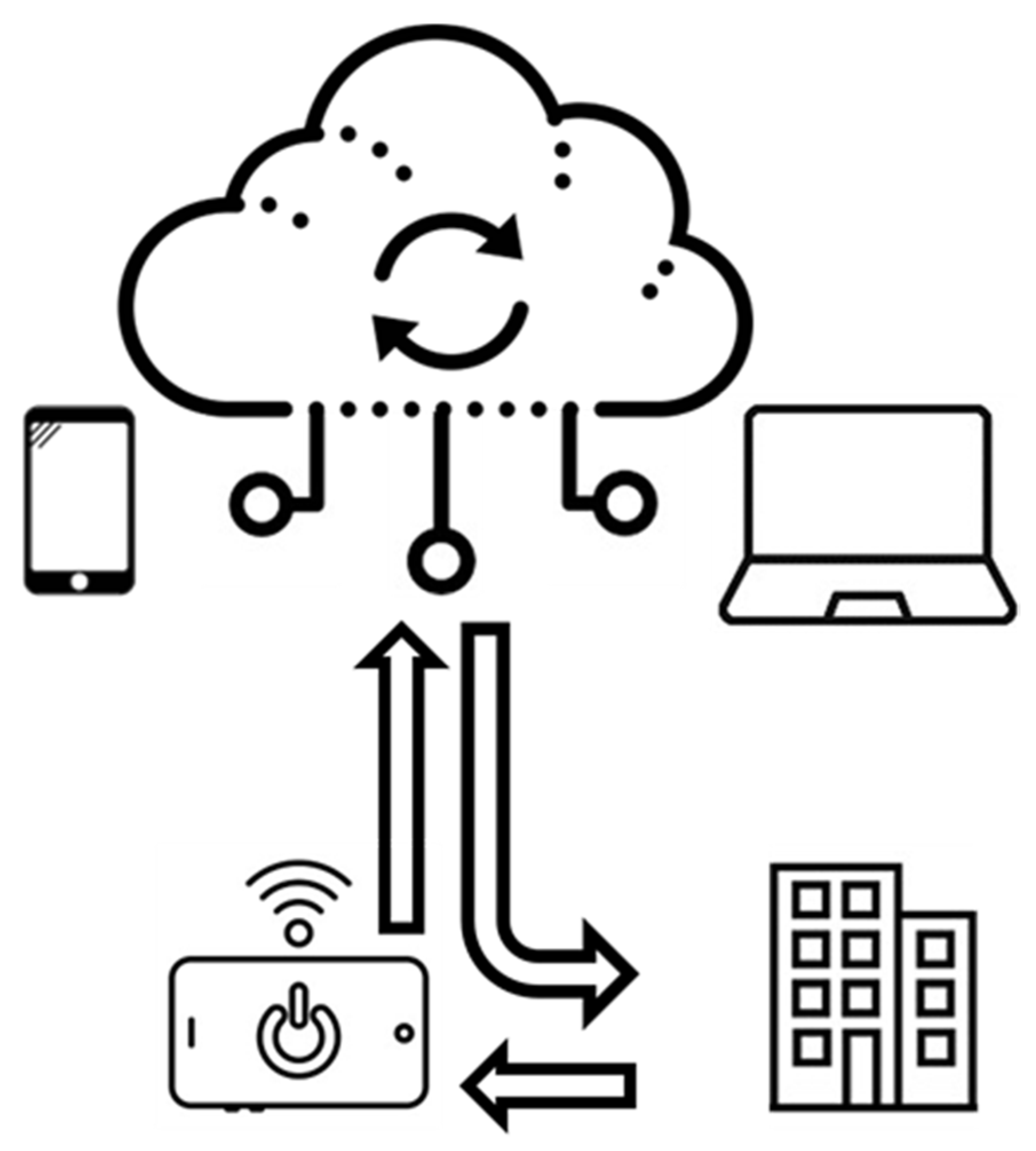
The interconnection of clonic devices with other systems favors the use of the Internet of Things (IoT) and data storage in the cloud. These enabling technologies allow wirelessly collected data to be evaluated for interpretation, in real time or deferred, for a real monitoring and control of the IAQ [79,80]. This has the potential to transform an existing building to be renovated into a smart building [81]. Several researches have studied the application of IoT for IAQ control [82,83]. They stress the advantages of system integration with connections to smartphone applications, ease of installation and scalability as an element to achieve cost improvements [84]. In this regard, Marquez et al. [85] developed research on an IoT solution that monitors CO₂ concentration in smart buildings. In this way, the IAQ can be controlled and therefore, the health of the occupants be improved.

It can be noted that clonic devices present a series of limitations. These are related to the maintenance and calibration of the sensors assembled, the communication protocols, and their power consumption [86]. Fortunately, with the aim of creating devices that help to promote healthy, sustainable, and smart cities, considerable progress has been made in recent years dealing with these issues [79].

The first objective of this research was to design, develop, assemble, and prototype a low-cost clonic device to provide buildings [87] with smart functionalities in the IAQ field [88]. As indoor comfort is currently taking a back seat to the priority of maintaining safe CO₂ levels to protect from COVID-19, research focused on the use of CO₂ sensors. Another purpose addressed was the choice of the best location to place the clonic device. 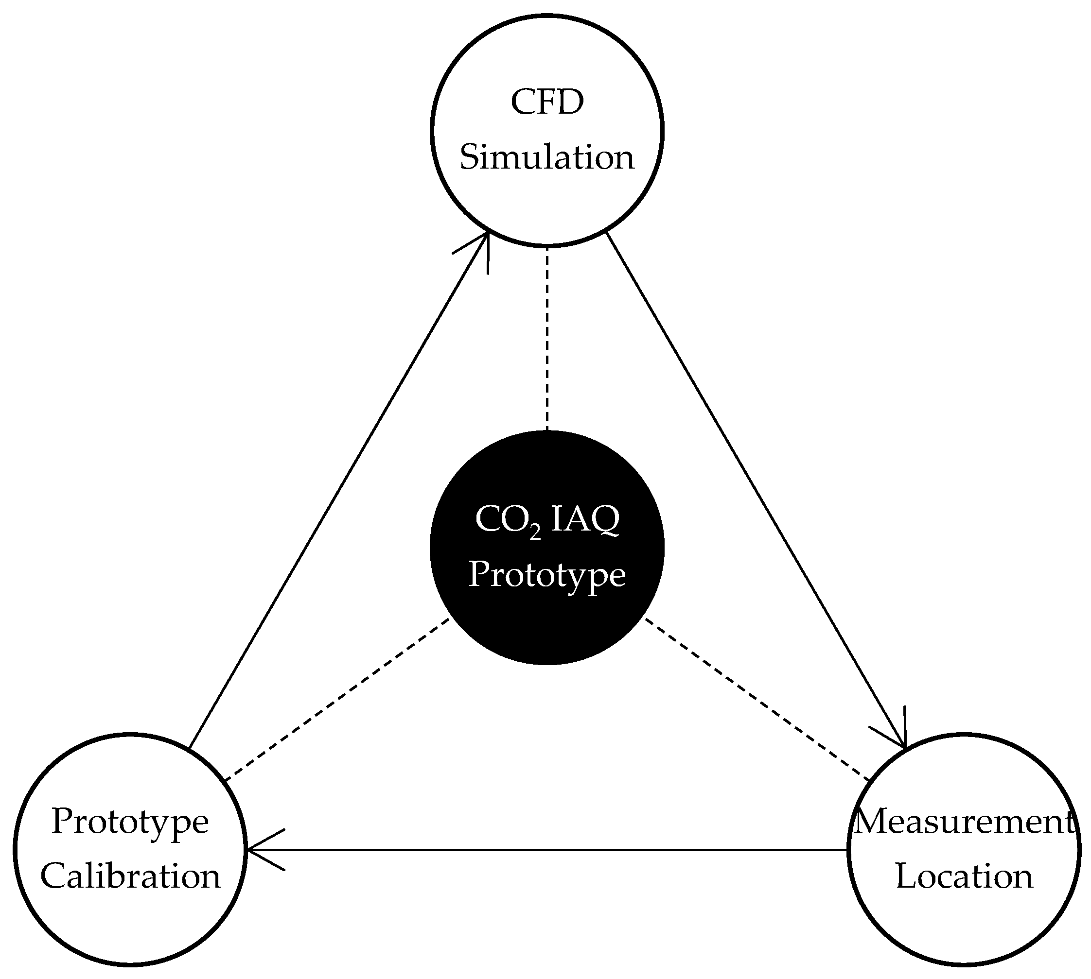To this end, computational fluid dynamics (CFD) simulations [89] were carried out in different scenarios (ventilation options) for a living space that was used as case study. It can be noted that, to the best of our knowledge, this has not been addressed before. Once the best locations for the placement and distribution of the instruments were determined, an experimental study was performed. Data were obtained with a calibrated equipment that was used as a reference standard and also with the low-cost prototype device. Comparisons were then made to check if measurements were acceptable for IAQ monitoring and control. In summary, the three main objectives and their relationship are shown in Figure 1:

• CFD analysis of the interior air flows of a living space to establish the location of measurement points.
• Exhaustive analysis of the solution to design and develop the prototype.
• Calibration of the cloning device for proper data acquisition.

The main novel contributions of this paper can be summarised in the following four elements:

• Complete design, development, and prototyping of a clonic device for CO₂ measurement as a control and monitoring parameter for IAQ. This parameter relates to air renewals for minimizing the spread of COVID. We showed all the physical components (sensor, microprocessor board and connections) and the programming code necessary for its operation.
• Description in detail the calibration protocol. In this paper, we used the KIMO HQ-210 commercial instrument as a reference standard for the clonic device. However, other instruments of similar characteristics with a calibration certificate from a laboratory legally accredited for this purpose could have been selected. In this context, we showed how to prepare a clonic device to properly measure CO₂ concentration.
• Process of all collected data in the cloud for further analysis and possible connection to other smart systems in the building. Therefore, we showed the applicability of the device to control and monitor CO₂ concentration and even act, if required, on HVAC systems.
• Definition of a methodology to obtain the best location of sensors for data collection. For this purpose, a CFD analysis was carried out in different scenarios of a case study. In this way, we improved the layout suggested by the different standards, which were limited to establishing separation values for the envelope (boundary) of the room without considering the air flows caused by the renewal of the interior air.

In summary, we showed for the first time, to the best of our knowledge, all the details of the components of the clonic device so that it can be cloned by anyone interested in the “do it yourself” philosophy. It also incorporated open source programming code, allowing other researchers to replicate the research and generalize this contribution to the scientific community and society. Furthermore, the use of the CFD methodology provided the most suitable points to determine the CO₂ concentration in the space to be studied, eliminating points that could generate distortions in the control and monitoring systems. In addition, using an open-source system allowed the connection with other smart building systems, which in the COVID-19 era can be considered a preventive measure to analyze IAQ.

2. Materials and Methods

This section describes the methodology used in the research, including its application in a case study. The methodology is primarily based on the use of CFD to determine the positioning of the CO₂ measurement system, for which simulations were carried out to identify those places where there is no air renewal. Next, it is necessary to design, configure, and develop a programmable clonic device.

The starting point was to select the living space where the prototype will be tested. A single-family house was taken in which a single bedroom was to be used as a study room. In this space, the calibration of the clonic device was carried out using a high-precision and high-cost calibration instrument. For this purpose, different assumptions and scenarios were defined, which are described in detail further in the next sections. Furthermore, this room is the space used to perform the CFD simulations. For obtaining the main results, the geometry was modeled in CATIA V5, and the different boundary conditions defined in ANSYS Discovery 2021 R2. These results allowed us to identify the best location of the programmable clonic device inside the room.

2.1. CFD Analysis

CFD is an area of engineering knowledge that belongs to the computer aided engineering (CAE) simulation programs. These analyses allow the numerical and visual simulation of flows, heat transfer, and even chemical reactions. These simulations and analyses are increasingly used to characterise living spaces, determining how the ventilation is operating and therefore the level of existing pollution. In short, CFD analysis helps to detect where the air is fouled. Thanks to this, preventive measures can be taken to avoid air quality risks [90]. These rises may be due to an increase in the number of people inside living spaces or a lack of ventilation in them [86,90]. In this study, CFD simulations helped to detect CO₂ concentration.

For this research, two different software packages were used: ANSYS Fluent 2021 R2 and ANSYS Discovery 2021 R2 (available at www.ansys.com). ANSYS Fluent was used for static and dynamic simulations. In addition, ANSYS Discovery was used only for dynamic simulations. The main features that had to be selected are:

• Dimension: 3D.
• Display options: Display mesh after reading.
• Options: Double precision.
• Processing Options: Serial.

To begin with the analysis, the geometry and boundary conditions had to be previously defined to establish the convergence of the solution [86]. These boundary conditions were related to CO₂ concentration and ventilation flow, helping to determine the location of the measurement instruments. The case study analyses the indoor atmosphere of a medium-sized room in a single-family house was simulated. In order to perform it, a series of conditions and restrictions had to be established:

• The building is located in Medina Sidonia, a village in the province of Cadiz (southern Spain). Its height above the sea is 337 m. In addition, its coordinates are as follows: longitude 5°55′37.81″ W; and latitude 36°27′25.02″ N.
• The usual outdoor pollution levels are low, thanks to its location near Alcornocales Natural Park on the town periphery. In some previous measurements with the standard reference equipment, the CO₂ concentration ranged from 380 to 410 ppm under different conditions of traffic, industrial activity, and prevailing winds. It can be noted that although some of the values are even lower than those indicated by the technical report “CEN/TR 16798-2”, a value of 400 ppm is assumed as the average outdoor concentration, as suggested by the report.
• The characteristic wind in this area comes from the east. As the main opening is in the southeast direction, the room received an adequate amount of fresh air.
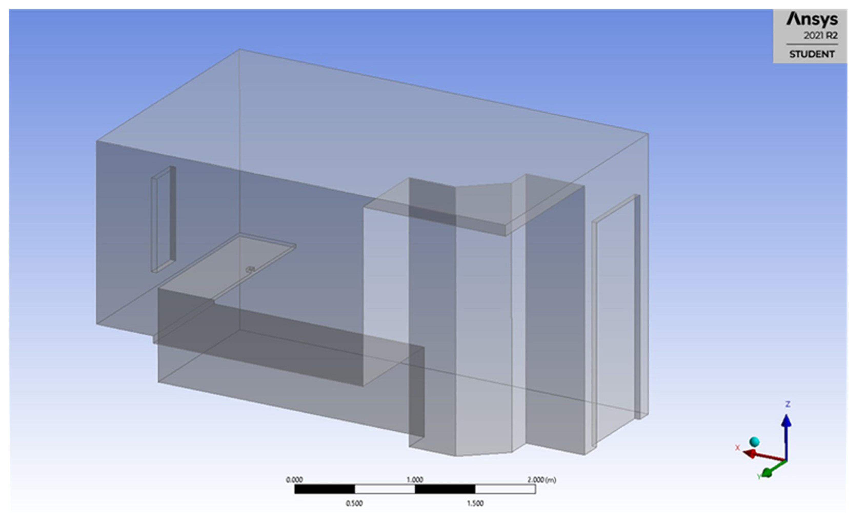
• The room consists of a rectangular enclosure of average dimensions (3.9 × 2.4 × 2.5 m). The geometry allowed the simulations to be carried out easily. It can be noted that this is a factor that directly influences the meshing performed by ANSYS. In addition, the boundary conditions defined refer to the amount of air entering the room, which was considered constant in the defined scenarios.
• Only one person lives in the room. No additional CO₂ emissions were considered that could have an impact on the defined boundary conditions.
• The test room is not forced ventilated and has no HVAC systems to renew the air inside. Therefore, ventilation is natural, with air being renewed through the openings in the envelope. The room has an exterior sliding window (height 0.93 m and width 0.63 m by leaf) and an interior door (height 2.03 m and width 0.72 m) that communicates with the rest of the rooms in the building.
• We intended to locate a clonic device inside the room. For this purpose, it was essential to determine the areas where there is no air renewal, as well as the presence of vortices that may affect data collection.

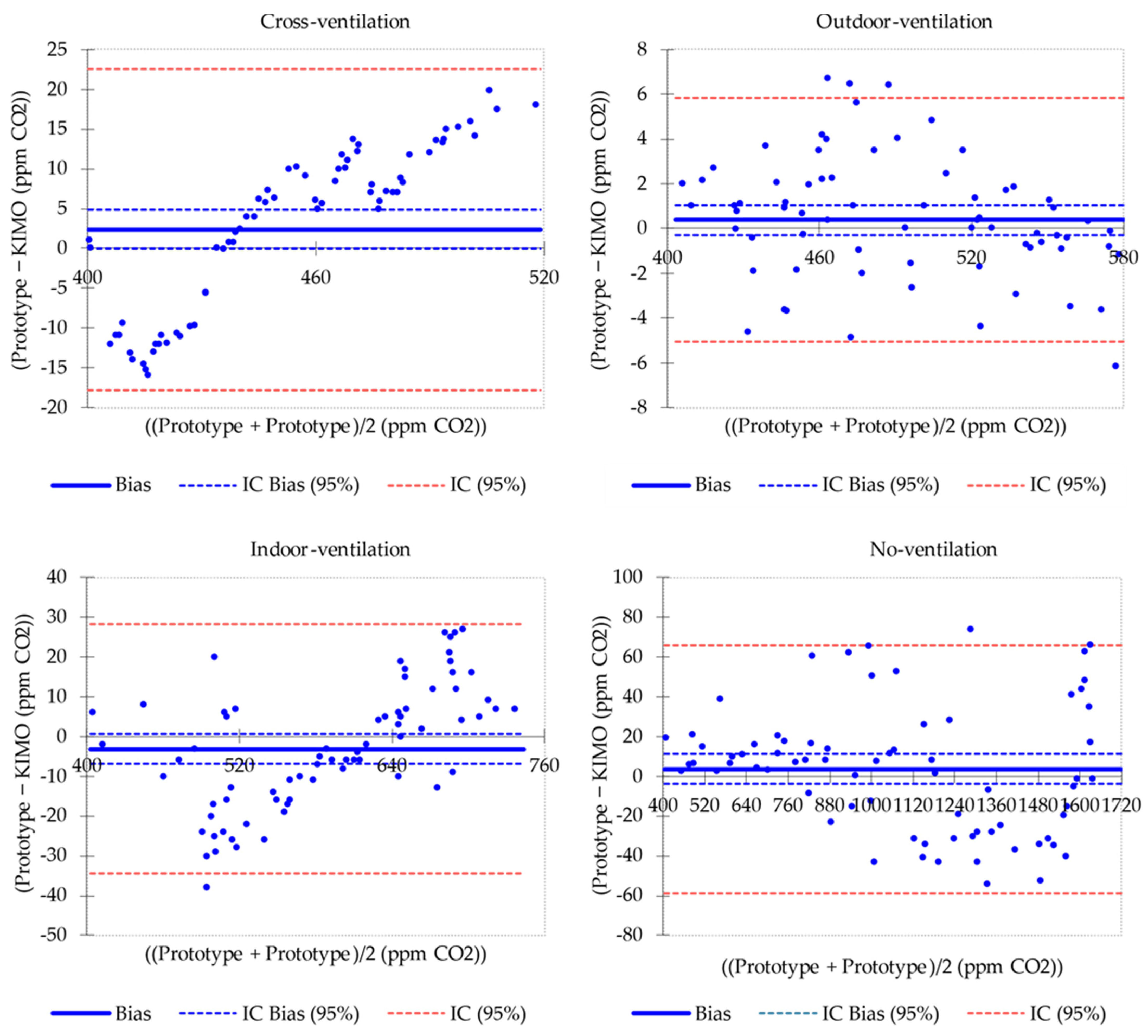
Four scenarios were defined for the CFD analysis. This made four situations possible: closed window and door (no ventilation), closed window but opened door (internal ventilation which is an indirect ventilation through other spaces that are also being renovated), opened window but closed door (external ventilation) and opened window and door (cross ventilation). In each of them, it was essential to guarantee the continuity of the simulation. For this purpose, an air inlet and outlet opening had to be established.

• Scenario 1 (cross-ventilation: Air renewal with opened window and door). Air enters through the window. At the same time, air exits through the door.
• Scenario 2 (outdoor-ventilation: Air exchange with opened window and closed door). In this case, the door is closed. The air enters through the window and exists through the lower area of the door (due to its permeability). In this way, continuity is ensured.
• Scenario 3 (indoor-ventilation: Air renewal with opened door and closed window). Opposite case to the previous one.
• Scenario 4 (no-ventilation: door and window closed). No air is exchanged. In this case, only the concentration of CO₂ metabolically generated by the occupant is simulated. To ensure continuity, it is necessary to define their permeability.

The boundary conditions refer to the mass flow of air and CO₂ entering and exiting the room. For the analysis of the renewal of IAQ in the presence of a CO₂ emission source, the geometry was created using DesignModeler, defining the inlets and outlets for each of the gases considered. A turbulent flow was modelled, specifically governed by the equations of the k-omega SST turbulence model. The physico-chemical characteristics of the gases involved were taken from the ANSYS database, activating the “Species” model. The composition of exhaled air is 78.6% N₂, 1.8% H₂O, 15.6% O₂ and 4% CO₂. Accordingly, the mass flux of CO₂ emitted by a person breathing is small. For instance, the amount of air emitted by a person while performing activities at rest is approximately 0.0004 kg/s [91]. This emission was considered to be ideal and constant. Although a mesh with small elements would lead to a more precise solution, this increased the calculation time. This mesh was defined with small triangular elements which were between 0.05 and 0.1 m in size. In addition, the air inlet was considered to be the exterior window opened, and the air outlet was considered to be the interior door opened. To determine the mass flow, the following Equations (1) and (2) were used:

$$V_i=L_i\times W_i\times H_i$$

(1)

where:

• $V_i\mathrm{is}\mathrm{the}\mathrm{volume}\mathrm{of}\mathrm{the}scenari{o}_i$
• $L_i\mathrm{is}\mathrm{the}\mathrm{length}\mathrm{of}\mathrm{the}scenari{o}_i$
• $W_i\mathrm{is}\mathrm{the}\mathrm{width}\mathrm{of}\mathrm{the}scenari{o}_i$
• $H_i\mathrm{is}\mathrm{the}\mathrm{heigth}\mathrm{of}\mathrm{the}scenari{o}_i$

$$M_f=D_{air}\times V_f$$

(2)

where:

• $D_{air}\mathrm{is}\mathrm{the}\mathrm{density}\mathrm{of}\mathrm{the}\mathrm{air}\mathrm{at}\mathrm{temperature}\mathrm{of}25°\mathrm{C}$
• $M_f \mathrm{is}\mathrm{the}$ Mass flow
• $V_f \mathrm{is}\mathrm{the}$ Volumetric flow

Applying the values from the case study:

$$\begin{gathered} V=3.9\times 2.4\times 2.5=23.4 {\mathrm{m}}^3, \\ {D}_{air} \left(25 ℃\right)=1.3 \mathrm{Kg}/{\mathrm{m}}^3 \end{gathered}$$

In the first simulation, cross ventilation: A static analysis was performed in which the gas present in the indoor atmosphere was air. Similarly, for the inlet and outlet opened, the incoming and outgoing gas was also defined as air. For the inlet, the mass flow considered was 0.024 kg/s, which corresponds to three renewals per hour for the volumetric flow. The output of this simulation was defined by the “outflow”, which allowed the law of conservation of mass to be satisfied: the entire mass flow of air entering through the window passes out the door. In addition, CO₂ was injected, simulating the constant exhalation of a person in a resting state.

In the second simulation, outdoor ventilation: The renewal airflow was performed through the window opened (one sliding leaf), the door being closed. A static analysis was carried out in which the gas present in the indoor atmosphere was air. Similarly, through the inlet opened, the incoming gas was air. The mass flow rate considered corresponded to one point five hourly renewals for the volumetric flow, then the mass flow was 0.012 kg/s. In this case, a slit at the bottom of the door (its clearance) was defined as the exit. This allowed for continuity within the room. The output of this simulation was defined by the “outflow”, which allowed the law of conservation of mass to be satisfied: all the mass flow of air entering through the window opened passes out the door slit. Analogous to the previous simulation, CO₂ was injected, simulating the constant exhalation of a person in a resting state.

In the third simulation, indoor ventilation: The renewal air flow was performed through the door opened, the window being closed. A static analysis is carried out in which the gas present in the indoor atmosphere was air. Similarly, through the inlet opened, the incoming gas was air. The renewal air mass flow rate was 0.008 kg/s. In this case, a slit in the side window (its permeability) was defined as the exit. This allowed for continuity within the room. The output of this simulation was defined by the “outflow”, which allowed the law of conservation of mass to be satisfied: all the mass flow of air entering through the door opened passes out the window slit. Analogous to previous simulations, CO₂ was injected, simulating the constant exhalation of a person in a resting state.

2.2. Professional Equipment

To select the professional equipment to be considered as a reference standard, a series of characteristics related to its weight, dimensions, and price were required. To begin with, the equipment must be certified by a recognised accredited agency. In addition, they must include human and battery autonomy, which allows measurements to be taken over long periods of time (greater than 50 h). A probe with infrared sensor for CO₂ measurement must be coupled. A wireless connection between the equipment and the probes available must be provided. The measurement modules must operate with different parameters and temperature ranges (from −20 °C to +80 °C). Finally, the professional equipment must measure in working environments with neutral gases. Among those available on the market, a KIMO HQ-210 was chosen. The equipment is supplied with a calibration certificate for the temperature, hygrometry, and CO₂ concentration probes (code NEM1700592 SCOH 112).

2.3. Low-Cost (Clonic) Device

Main advantages and disadvantages of the commercial equipment were considered as a reference to select the main components of the clonic device. In this regard, two elements were fundamental to create it: a sensor to monitor the concentration of CO₂ and an electronic motherboard that allows the processing of atmospheric data. In order to select the most suitable components, a series of criteria matrices were used to score the characteristics considered, which are detailed below.

Firstly, a CO₂ sensor was chosen, for which its main characteristics evaluated were:

• Measurement range: it should be high (0–5000 ppm).
• Accuracy: it should be less than ±0.1%
• Capability of monitoring: it should measure one IAQ gas. In this case, CO₂.
• Sensitivity: it must provide high sensitivity and speed of response (in minutes).
• Heating time.
• Price: it should be less than EUR 30.

Four different sensors were considered: Amphenol Advanced Sensors Telaire T6713, Sensirion SCD30, DFRobot SEN0219, and Amphenol SGX Sensortech MiCS-VZ-89TE. The result of the criteria matrix is shown in Appendix A. After performing the criteria matrix (see

Table A1. Criteria matrix for sensor selection.

Factor	T6713	SCD30	SEN0219	MiCS-VZ-89TE
Measuring Range	2	2	2	0
Accuracy	1	1	1	0
N° parameters	2	0	2	2
Response speed	1	2	1	2
Warm-up time	2	2	2	2
Price	0	0	1	2
Total	8	7	9	8

), the most suitable sensor was the SEN0219. This is an analog sensor capable of monitoring CO₂ in an exclusive way by using non-dispersive infrared (NDIR) principle to detect the existence of CO₂ in the air. It features a long life, high resolution, accuracy and sensitivity, as well as a medium response speed. In addition, it is easy to install on any microcontroller and its price is relatively low (between EUR 30 and EUR 60).

Secondly, the selected motherboards included the Raspberry Pi Model B+ microcomputer and the Arduino MEGA 2560 R3 and ELEGOO MEGA 2560 R3 microcontrollers. Due to the similarities between the Arduino and ELEGOO microcontrollers, ELEGOO was considered because of its lower price. Their main factors evaluated were:

• General characteristics.
• Software and hardware.
• Innovation.
• Interconnection.
• Price.

The result of the criteria matrix is shown in Appendix A. Although both boards were suitable and had the right features for mounting the programmable device (see

Table A2. Criteria matrix for sensor selection.

Characteristics	ELEGOO MEGA 2560 R3	Raspberry Pi 3 Model B+
Dimensions	101.52 × 53.3 mm	85 × 53 mm
Memory capacity	8 kb	1 Gb
Language	C, C++	Python, C, Java, Javascript, …
Processor speed	16 MHz	1400 MHz
Inputs and outputs	54 digital I/O pins and 16 analog inputs	40 pins (known as GPIO)
Other connections	USB Type B	4 USB ports, HDMI, Internet, Memory card
Price	EUR 13.99	EUR 30–40

), ELEGOO MEGA 2560 Rev3 had a more intuitive and user-friendly software interface. The C++-based programming language allows fast programming of the SEN0219 sensor, as it is designed for implementation on microcontrollers. Although Raspberry Pi has many advantages, this project could not make full use of them. Additionally, the programming language (mainly Python, which is one of the base programming languages of Raspberry Pi) is complex and designed for expert programmers. After performing the criteria matrix (see

Table A3. Criteria matrix for sensor selection.

Factor	ELEGOO MEGA 2560 R3	Raspberry Pi 3 Model B+
Characteristics	1	2
Software/Hardware	2	0
Innovation	2	2
Interconnection	2	2
Sensor integration	2	1
Price	2	2
Total	11	9

), the most suitable motherboard was the ELEGOO MEGA 2560 Rev3.

2.4. Programming and Calibration of the Device

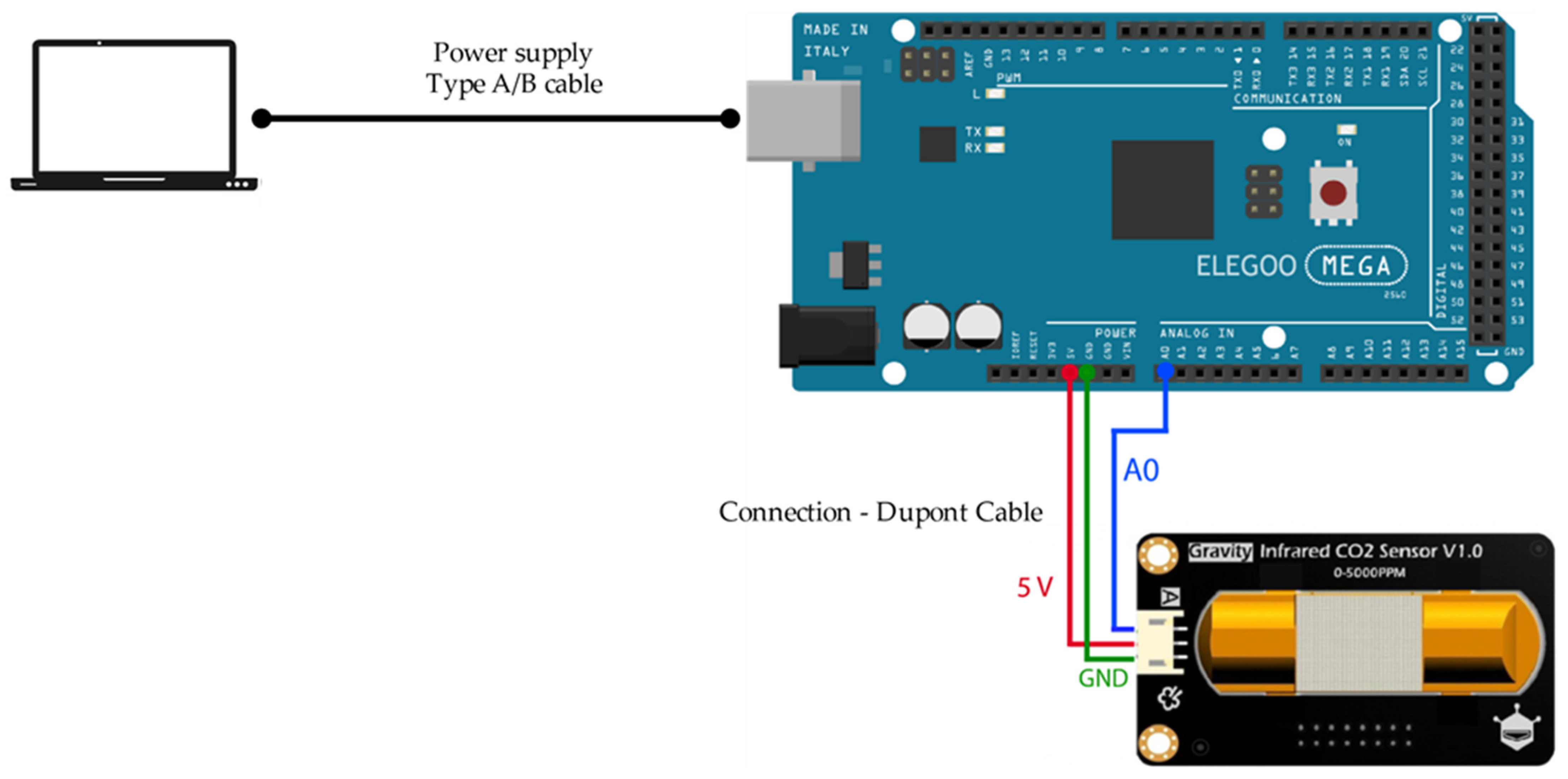
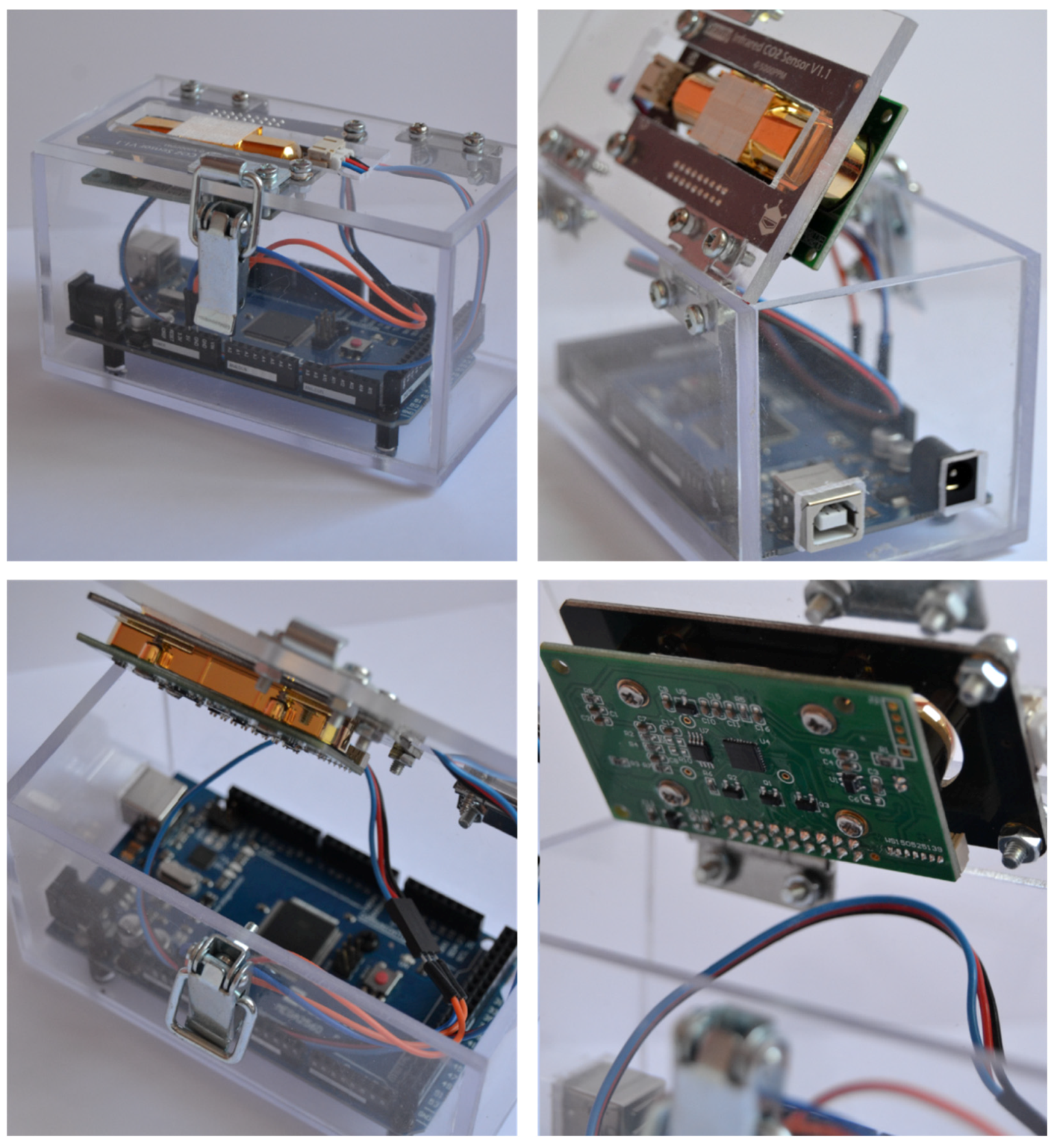
Once the motherboard and the sensor to be used were selected, they were assembled and programmed. The SEN0219 CO₂ sensor could be easily connected to the ELEGOO MEGA 2560 R3 microcontroller (see Appendix B, Figure A1). The software and programming language used was Arduino. The prototype is shown in Figure 2.

Data captured by the sensor in the Arduino Serial Monitor were stored in a Microsoft Excel spreadsheet. For this purpose, additional programming code was carried out in the Visual Studio Code editor. This allowed the data stored to be analysed from time to time. This parameter was defined in the programming code depending on the monitoring needs. Once the system was ready, the next step consisted of the calibration of the zero point (which is based on the idea that if the sensor is placed into a 100% concentration of an alternate gas, the sensor reads absolute zero). This process was performed according to the datasheet of the manufacturer of the sensor, by shorting the circuit between the HD and GND pins for 7 s at least, but previously ensuring that the sensor was stable for more than 20 min at fresh air (400 ppm ambient environment). However, other alternative methods could have been used such as exposing the sensor to a gas with a known CO₂ concentration or to a gas with no CO₂ present. After that, since it was intended as a low-cost device, it was not required to correct the input voltage and gain (offset voltage) unless anomalies were detected in the readouts. Finally, if measurements were not within the tolerance range, then an adjustment inside the calibration was required. This was done by linear regression.

The calibration line was included in the programming code (see Appendix C). It relates the CO₂ concentration (in ppm) with the voltage values (in mV) captured by the sensor. Both parameters were related by two constants (C₁ and C₂ in Equation (3)), which were provided by the DataSheet of the analog sensor. These constants needed to be calculated in order to modify the regression line and achieve the adjustment within the calibration of the programmable device. The calibration line consisted of the following form:

$${\mathrm{CO}}_{2i}=\left(C_1\times V_i\right)-C_2$$

(3)

where:

• ${\mathrm{CO}}_{2i}$ is the concentration in ppm unit at “i” time.
• $V_i$ is the voltage in mV unit at “i” time.
• $C_1$ is the first constant in linear regression line.
• $C_2$ is the second constant in linear regression line.

The regression line obtained allowed the calibration process of the clonic device to be carried out. An analytical process of data collection is explained below. To achieve this, the data from the device was compared with a calibrated highly accurate and costly measuring instrument. To be precise, the KIMO HQ-210 equipment from KIMO Electronic Pvt. Ltd. (Mumbai, India), was selected. It consists of two probes capable of monitoring CO₂, temperature, and humidity. The error of this measuring instrument was reflected in the calibration certificate provided by the manufacturer. This error was also considered in the error of the clonic device calibration. Prototype calibration was also possible thanks to the collection of a lot of data from both the sensor device and the KIMO equipment. To obtain the calibration line, the voltage measured by the sensor was related to the exact and real concentration value provided by the reference standard. This line changed every time a new calibration was performed. To be accurate, three rounds of calibration were needed to achieve a maximum target error of less than 10%.

All the calibrations were performed in the same location during a 9 h measurement interval. This location was the same as the one considered in the CFD simulations. The SEN0219 sensor device and the KIMO equipment were placed side-by-side. Only the characteristics considered were changed for obtaining the minimum error for each calibration. Data collection by the sensor device and the KIMO equipment was carried out at regular intervals of 5 min (which provided 108 measurement points each). A shorter time between measurements was beneficial to obtain more data, helping to obtain a more accurate and successful calibration line. Additionally, this time could be linked to the resolution of the IAQ monitoring device. A longer time between data collection meant that changes in CO₂ concentration were neglected.

Calibrations compare the experimental data from the KIMO equipment with the prototype estimates. To validate these comparisons, different error rates are used. This allows to observe how well the prototype device reproduces the behavior of the reference standard equipment. Several indices for validating models are reported in the literature, which can be classified according to their dependence on the scale of the compared signals. To begin with, errors that depend on the scale [92] such as the mean absolute error (MAE) used by [93] which measures the average magnitude of the error between the measured data by the equipment and the data estimated by the device, the mean error (ME) used by [94] which measures whether the device measures whether the device overestimates or underestimates the measured data, and the root mean square error (RMSE), used by [95] which weights the forecasts that are farthest away from the measured value by the equipment. Additional examples include the errors that do not depend on the scale [96] such as the mean absolute percentage error (MAPE) used by [97] which measures the average percentage error of the estimates and the best fit index (FIT) used by [98] which compares the measured and estimated data with respect to the average of the measured data.

It can be noted that the coefficient of determination (R²) only measures the proportion of the variance in the dependent variable that is predictable from the independent one [99]. In addition, R² is invariant for linear transformations of the distribution of the independent variables [100], so that an output value close to one does not always produce a good prediction regardless of the scale on which these variables are measured. In this context, indicators as MAPE are recommended when it is more important being sensitive to relative variations than to absolute variations [101]. However, although scale-independent errors are widely used in the literature, since they are used when comparing data with different scales, the weighting of the larger-scale error causes adjustments with larger deviation the higher the CO₂ concentration to penalize against others. For instance, RMSE gives a relatively high weight to large errors since the errors are squared before they are averaged, so that it is useful when large errors are particularly undesirable [102].

2.4.1. First Round of Calibration

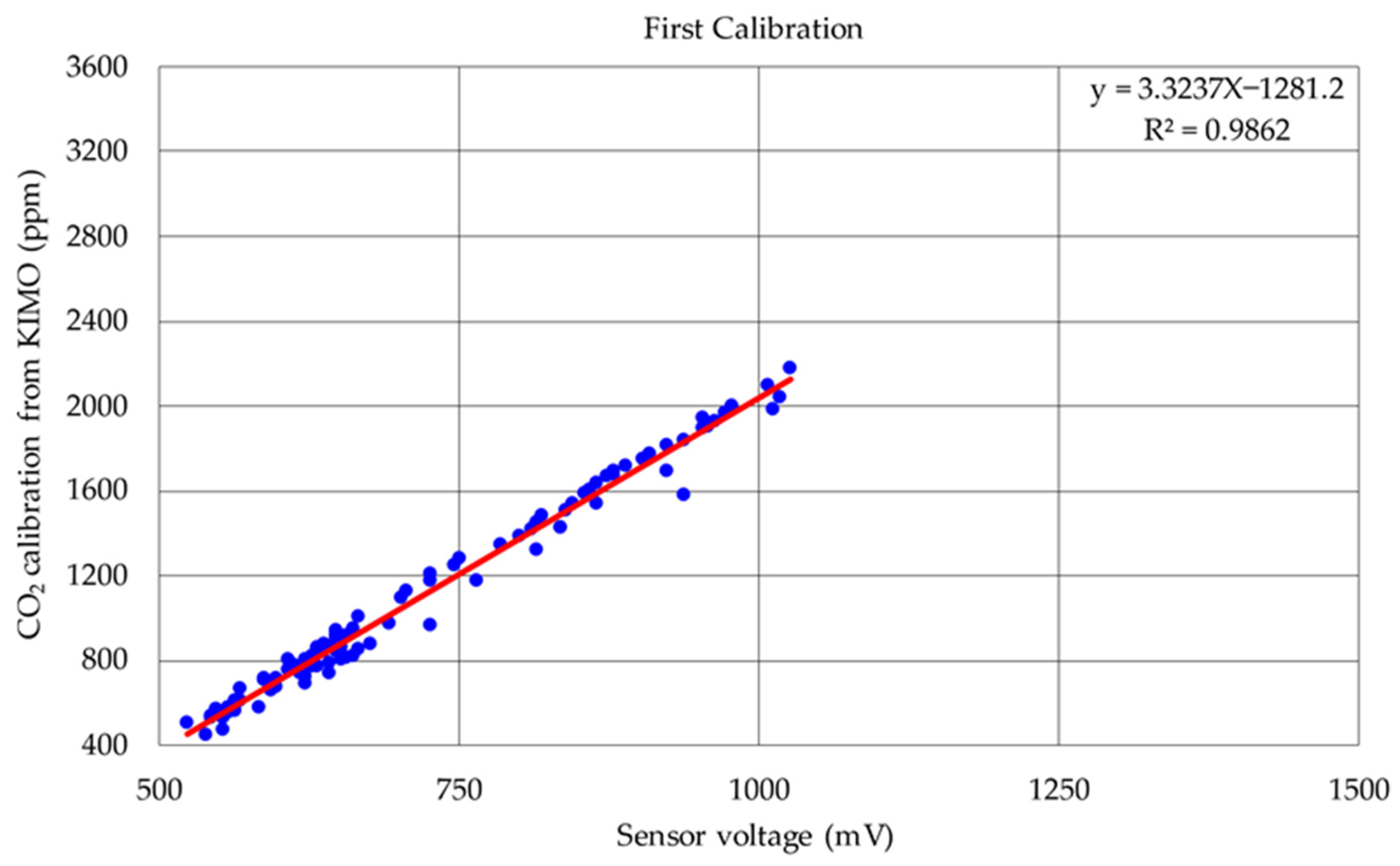
This was the first contact with the sensor. The upward and downward trend of the concentration recorded by the sensor corresponded to those obtained by the KIMO equipment. Even so, there was a large error that must be resolved by calibration. Figure 3 shows the first calibration line. This error became larger in case of high CO₂ concentrations. This is shown in Figure 4. However, after the adjustment, the error between the prototype device and the KIMO equipment decreased significantly, as shown in

Table 3. Statistical parameters related to the errors of the first calibration.

First Calibration	Datasheet	After Adjustment
	(y = 3.1249x − 1251.6)	(y = 3.3237x − 1281.2)
MAE	114.74 ppm	43.03 ppm
ME	111.85 ppm	0.05 ppm
RMSE	127.92 ppm	55.41 ppm
MAPE	11.10%	04.49%
FIT	72.32%	89.46%
R2	98.62%

. Therefore, a further calibration had to be performed, taking into account these considerations:

• The atmosphere at the time of data acquisition must be as stable as possible. Sudden changes in temperature, humidity, or CO₂ must be avoided.
• The clonic device and the KIMO equipment are placed elsewhere. Areas close to the window or door of the room must be avoided. This makes it possible to ensure the previous point considered.
• The number of data collected (minimum 60) must be increased.

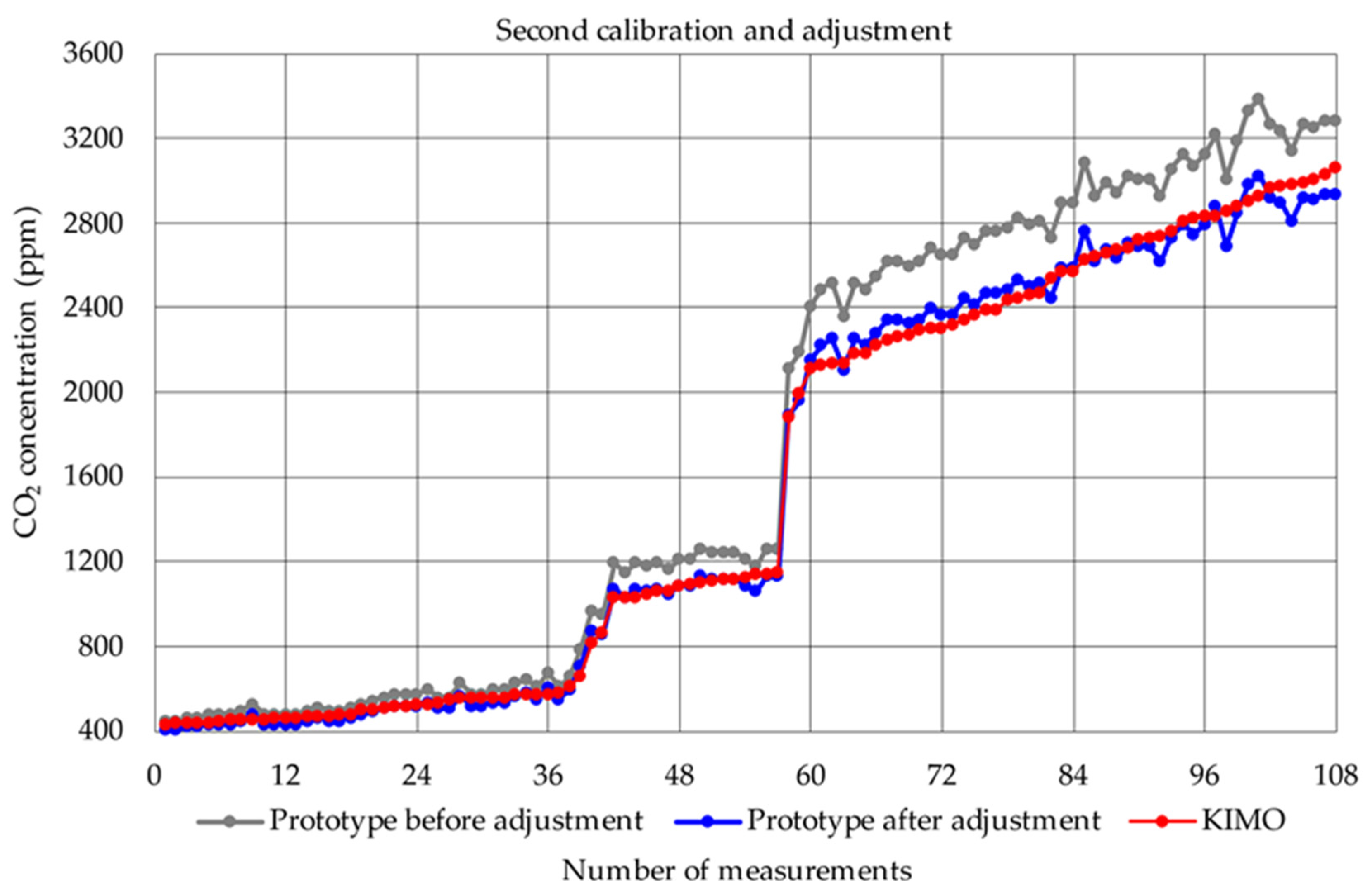
2.4.2. Second Round of Calibration

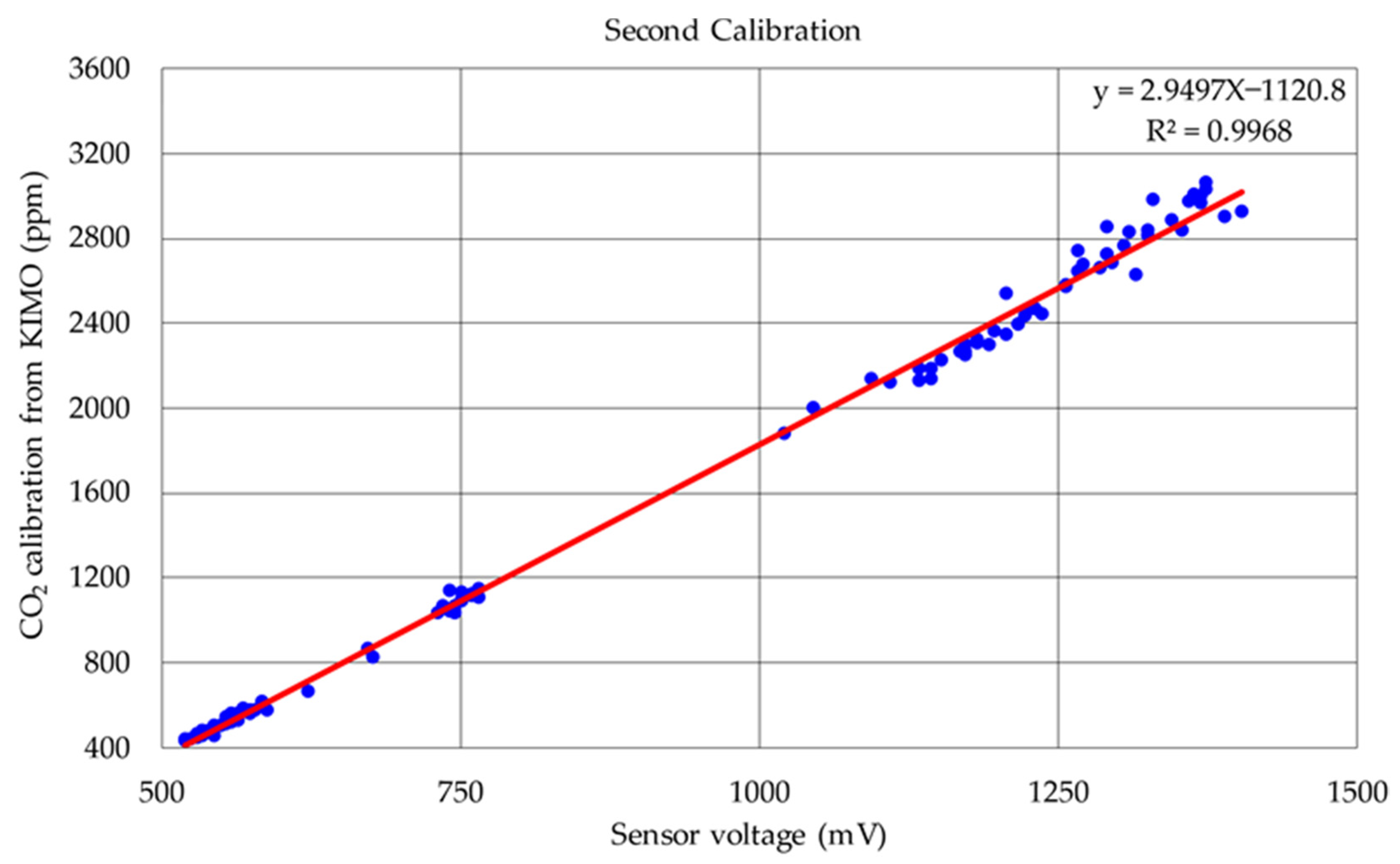
Since the errors after the first calibration were greater than 10%, a second calibration was performed. Although with the adjustment the errors could be lowered, there was no guarantee that under other conditions this adjustment could be contradictory. With the adjustment after the first calibration, the second calibration was performed. In the subsequent data, there was still a significant difference between the values monitored by the two instruments. Figure 5 shows the second calibration line. This still resulted in an average error of more than 10%, as shown in

Table 4. Statistical parameters related to the errors of the second calibration.

Second Calibration	Before Adjustment	After Adjustment
	y = 3.3237x − 1281.2	2.9497x − 1120.8
MAE	180.34 ppm	41.65 ppm
ME	−180.34 ppm	1.17 ppm
RMSE	225.37 ppm	55.17 ppm
MAPE	10.44%	2.97%
FIT	82.70%	95.56%
R2	99.68%

. Despite this, progress was favourable (when adjusting) and the graphs began to look similar in low and medium CO₂ concentration, as shown in Figure 6. In addition, several conclusions could be drawn from this calibration:

• The occupant of the living space must be far away from both instruments (prototype and equipment). This avoids falsification of data by possible direct exhalation on them.
• Data collection must not be started until 15 min after a change in the atmosphere. These changes are caused by the opening of door and window. After 15 min, the atmosphere becomes stable again.

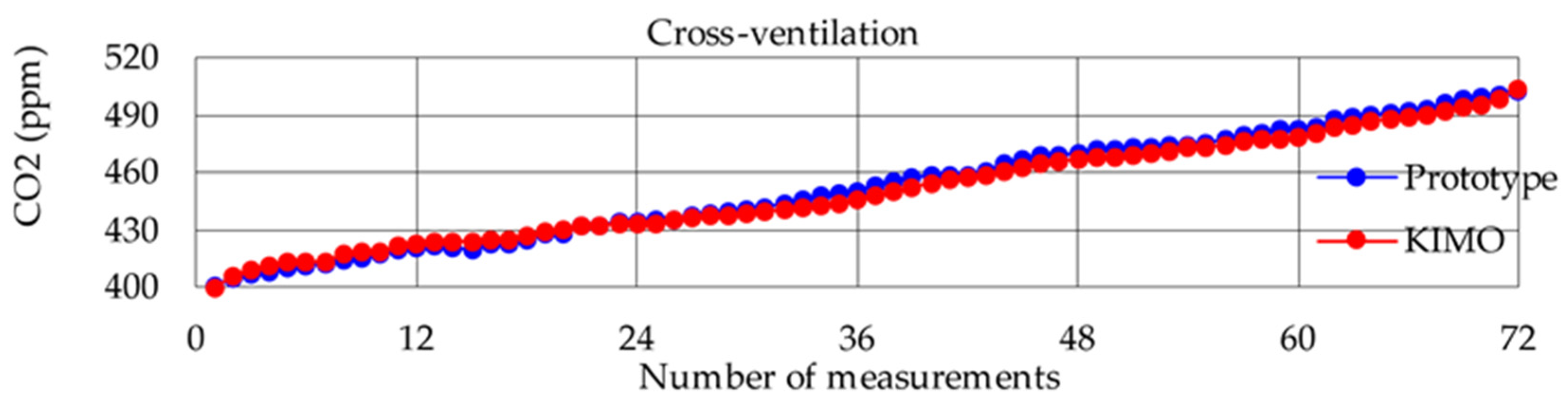
2.4.3. Third Round of Calibration

All considerations from the two previous calibrations were made. With the adjustment after the second calibration, the third calibration was performed. The average error obtained was below 10% even before the adjustment, as shown in

Table 5. Statistical parameters related to the errors of the third calibration.

Third Calibration	Before Adjustment	After Adjustment
	2.9497x − 1120.8	y = 2.9713x − 1150.3
MAE	29.29 ppm	27.45 ppm
ME	−13.94 ppm	0.01 ppm
RMSE	35.17 ppm	32.17 ppm
MAPE	3.11%	3.03%
FIT	90.23%	90.96%
R2	99.31%

. Therefore, this calibration could already be considered suitable to start testing the different scenarios. Figure 7 shows the third regression line after calibration. As a result, the difference between the clonic device and the KIMO equipment was small, as shown in Figure 8. With this milestone, the calibration process was completed. However, to ensure that the clonic device measured constantly, regularly, and correctly, a preventive maintenance had to be scheduled. It is recommended to carry out calibrations every short period of time. This allows one to transform it into a predictive maintenance, since both absolute and relative error rates can be studied.

3. Results and Discussion

For presenting the results of the research and their discussion in an organised structure, the diagram presented in Figure 9 is followed. Then, the most relevant milestones involved in all phases of the research is summarised.

3.1. Phase 1: Perform CFD Simulations

As indicated in the previous section, the study was performed in four scenarios. They were those corresponding to the same living space of 9.4 m² with a unique occupant in soft sorting activities (minor than 6 MET), but in the following conditions:

• Cross-ventilation: space with door and window opened.
• Outdoor-ventilation: space with door closed and window opened.
• Indoor-ventilation: space with door opened and window closed.
• No-ventilation: space with door and window closed.

The hygrometric comfort conditions were considered acceptable in all simulations, with temperature (T) ranging between 17 °C and 25 °C and relative humidity (RH) between 40% and 70%. The room faces southeast (taking the plane of the window as a reference). As the characteristic wind in this area comes from the east, ventilation with an open window was satisfactory. Figure 10 shows the working space employed in the research. The room was modelled with Ansys 2021 R2 version software.

The main parameters considered in the simulations was the mass flow of incoming and outgoing air through the different openings and the concentration (or mass flow) of CO₂ from the metabolic exhalation of the occupant in the working space. Among four scenarios, cross-ventilation had the highest air renewal. This example could be extrapolated to public spaces that require a high air renewal rate to keep CO₂ levels low. Therefore, the location of measurement points was based on this scenario, as it was the most unfavourable. In this scenario, static and transitional tests were performed. For this purpose, an inlet air mass flow rate of 0.008 kg/s for each hourly renewal considered, depending on the scenario, was defined. Figure 11 shows the zones in the space where vortices are formed. It must be noted that these points were not suitable for the placement of the CO₂ sensors for IAQ control.

On the other hand, in the case of no-ventilation (Scenario 4), the same mass flow of air was considered and there was an increase of exhaled metabolic CO₂. The permeability of the door and window allowed for pressure balancing through minimal air renewal, which was considered. Figure 12 shows the simulation of this scenario for a period of 9 h. As can be observed, as time progressed, the CO₂ concentration in the working space became uniform, being higher in the areas close to the CO₂ emitter.

To decide a good sensor location in each of the four scenarios, the parameters for the mass flow of air from the concentration of CO₂ emitted by the people in the room measured and the ventilation were used. The amount of CO₂ reflected in all simulations performed was 0.0004 kg/s. However, the mass flow of air from the ventilation varied according to the scenario considered. Among all of them, the highest mass air flow came from the highest air renewal (Scenario 1, cross ventilation) with three renewals per hour, corresponding to a volumetric flow rate of 20 L/s per person. By studying the behavior of the turbulent flow by CFD, the vortices in the room were observed. These points were not suitable for sensor placement. On the contrary, in Scenario 4 (no ventilation), there was no air flow that caused vortices and the CO₂ concentration increased progressively, uniformly filling the volume tested. For this reason, the location of the sensors in Scenario 4 was the most demanding case for monitoring CO₂.

Figure 13 shows the three points selected among suitable ones for the CO₂ concentration measurement. They were placed in positions that do not correspond to the vortices nor currents of air, avoiding distorting measurement points. The red colour shows areas with high renewal, so that placing the sensors in these areas would distort the average level in the space. Despite the statements of previous research (to the best of our knowledge) and current legislation [103,104] which establish that measurements should be taken at 1.2 metres above the ground, equivalent measurements can be taken at higher or lower points, as they are not modified either by renovations or by CO₂ concentration in the most unfavourable scenarios. They are as follows:

• Location 1: right side wall at a height of 1.2 m above floor and a separation of 2.5 m from the wall of the door.
• Location 2: exterior wall (corresponding to the window) at a height of 2 m and centered in the gap between the left wall and the window.
• Location 3: left side wall at a height of 2 m above the floor and a separation of 1.5 m from the window.

As Location 1 complies with current legislation for all kind of activities that can be undertaken in the living space, this is the one selected for the series of measurements.

3.2. Phase 2: Study Low-Cost Elements for the Prototype

In this research, high-precision and high-cost instruments were used. However, other research with CO₂ measuring devices allowing CO₂ concentrations to be monitored less expensive were also analysed. The cheapest cost of these clonic devices, according to the latest research by Villanueva et al. [77], was EUR 75. The clonic device proposed has an open programming language, which is available in Appendix C. In addition, its price is approximately EUR 60, which is 20% cheaper. Therefore, users and construction companies can include it as an element for the transformation of buildings into smart buildings.

Regarding the parametric considerations, the error of the prototype compared to equipment calibrated was in the range between 0 and 7.49%. This error was much lower for Scenario 1 and comparable to commercial equipment in Scenario 4, according to research by Villanueva et al. [77]. The connection between prototype and cloud allows the collection of data and its further management, which is not possible with static devices that only provide a point measurement of the CO₂ concentration.

3.3. Phase 3: Calibrate the Prototoype

As detailed in the previous section, the calibration of the prototype was performed through iterations with regression lines. In successive calibrations, better and better fits were obtained. The last calibration determined that the error between the measurements obtained by the calibrated equipment (KIMO) and the prototype sensor device was less than the principal milestone of the project: less than 10%. Absolute indicators as RMSE as well as relative ones as MAPE could be used to check this. Therefore, after this process, a reliable prototype was obtained whose performance is comparable to other commercial or even clonic devices on the market such as those studied by Villanueva et al. [77].

3.4. Phase 4: Evaluate the Scenarios and Determine the Measurement Error

In this phase, a comparative analysis of the measurements made by the prototype device compared to those from the calibrated instrument was carried out. This statistical analysis of the data obtained was performed for each of the four scenarios. It consisted of capturing data every 5 min over a period of 6 h. The data obtained for the measurements in the four scenarios are shown graphically.

Figure 14 shows the data for Scenario 1 (cross-ventilation). It can be observed that the data corresponding to the measurement with the prototype coincided with those of the equipment calibrated. The minimum difference between the recopilated data (error) could be caused by cross-ventilation because the atmosphere was not completely steady. In addition, the CO₂ concentration was observed to remain at healthy levels, close to the IAQ values that can be achieved in outdoor environments. The amount exhaled by the occupant of the space had hardly any effect on the total concentration when the ventilation was cross-ventilation.

Figure 15 shows the data for Scenario 2 (outdoor-ventilation). The data from the measurement with the prototype matched those of the equipment calibrated. The CO₂ concentration was close to health thresholds in a small range, as the window being open, the airflow renewed the amount of clean air, keeping the scene in a healthy condition for the occupant.

Figure 16 shows the data for Scenario 3 (indoor-ventilation). The data from the measurement with the prototype match those of the equipment calibrated. Air renewal depends on the interior connection between the room and the rest of the building. Except for occasional measurements, the IAQ is considered to be adequate. In this case, in order to have more information, it would be necessary to perform the study of the entire building (including all the points where there could be air renewal).

Figure 17 shows the data for Scenario 4 (no-ventilation). The data from the measurement with the prototype matched those of the equipment calibrated. It can be observed how the amount of CO₂ increased to levels considered unhealthy. After approximately 50 min, concentrations close to 1000 ppm of CO₂ were obtained.

The instantaneous error of each measurement corresponded to the difference between the measurement obtained by the low-cost clonic device and the commercial instrument calibrated (KIMO). This measurement already incorporated the corrected measurement uncertainty of the KIMO instrument. Details of all measurements are included in the Supplementary Materials.

Simultaneous measurements were obtained with both the low-cost clonic device and the instrument calibrated (KIMO), which was employed as a reference standard. As stated before, these device measurements already included both the correction and the measurement uncertainty of the KIMO instrument. The values of the mean, minimum, maximum, and standard deviation values were studied.

Table 6. Comparative study of the sample with KIMO and prototype measurements.

Scenario	Device	Mean	Minimum	Maximum	Standard Deviation
Cross-ventilation	KIMO	450.88	400	504	27.00
	Prototype	452.49	401	503	28.98
Outdoor-ventilation	KIMO	494.07	405	585	51.55
	Prototype	494.45	407	582	50.66
Indoor-ventilation	KIMO	590.57	402	734	79.77
	Prototype	587.39	408	741	89.36
No-ventilation	KIMO	1087.69	401	1638	374.10
	Prototype	1091.24	420	1664	368.80

Note: The unit of measurement for CO₂ concentrations is ppm.

shows these values:

As explained before, an average outdoor concentration of 400 ppm was assumed, according to the technical report “CEN/TR 16798-2”. Then, normality (with the Kolmogorov–Smirnov test) and homoscedasticity (with the Fisher F-test) was probed.

Table 7. Normality and homoscedasticity proofs between KIMO and prototype (p-value).

Scenario	Kolmogorov-Smirnov	Fisher
Cross-ventilation	0.995	0.554
Outdoor-ventilation	0.95	0.883
Indoor-ventilation	0.491	0.341
No-ventilation	0.964	0.905

shows the values of the statistics for each of the scenarios.

Then, an equivalence test (the two-one sided test (TOST test)) was used to determine whether the means for both equipment measurements were close enough to be considered equivalent. Finally, the concordance between both samples was checked with the Bland-Altman plot, identifying any systematic difference between the measurements (as fixed bias) or possible outliers.

Table 8. Equivalence and concordance proofs between KIMO and prototype (p-value).

Scenario	TOST Top	TOST Lower	Bland & Altman
Cross-ventilation	<0.001	<0.001	0.153
Outdoor-ventilation	<0.001	<0.001	0.251
Indoor-ventilation	0.001	0.005	0.195
No-ventilation	0.031	0.024	0.347

shows the values of the statistics for each of the scenarios.

All the statistical indices shown in Table 7 and Table 8 as well as in Figure 18, indicate that there was normality and homoscedasticity between the values obtained by the prototype sensor device and the reference standard equipment. In addition, equivalence and concordance were also satisfactorily tested. Finally, the instantaneous error, which is the difference between the measurement of the low-cost prototype sensor device and the KIMO equipment, was calculated. This calculation was made for the 72 measurements taken every 5 min. The mean value was also considered. This study helped to determine the percentage error in each of the scenarios. Data are shown in

Table 9. Comparative study of the error with KIMO equipment vs. prototype device.

Scenario	Mean	Min	Max
Cross-ventilation	0.62%	0.00%	1.34%
Outdoor-ventilation	0.44%	0.00%	1.52%
Indoor-ventilation	2.34%	0.00%	7.39%
No-ventilation	2.38%	0.00%	7.49%

.

As can be observed, the comparative measurement error in all scenarios was less than 8%. If the experiment was performed in a case whose ventilation is maximum (cross-ventilation is 1 m/s), the values obtained were similar to the results of the study by Villanueva et al. [77] for other clonic devices.

3.5. Phase 5: Integrate into a Smart Building

Smart building infrastructures aim to maximise building efficiency in different fields of application. Specifically, this research focused on the assessment of IAQ to maintain a safe atmosphere for building occupants. However, given that the main issue at present day is the transmission of the COVID-19 disease, the parameter related to CO₂ concentration was used as a reference. For this purpose, a low-cost device was designed to transfer the captured data to the cloud. In this way, it is possible to retrieve the information for decision making or integration with other systems, such as those in charge of ventilation and air conditioning (HVAC) or even other systems for automatic opening and closing of elements for natural air renewal.

The other issue that has been addressed is the definition of a location for this equipment that allows it to be properly measured. In this regard, CFD studies have shown that, although the general recommendation of up to 1.2 m above the floor is correct, there are many more points where reliable data on CO₂ concentration averages can be obtained. In addition, vortices were determined and excluded from the potential location of the device, as its measurements would be distorted from the actual average. A functional scheme of the investigation is presented graphically in Figure 19. Integration with other systems in smart building was not addressed within the scope of this research, although this would allow better monitoring and control of these systems, promoting efficient energy use and helping to control indoor quality for disease prevention.

4. Conclusions

In the COVID-19 era, CO₂ concentration is the most important indicator related to IAQ to measure the degree of air pollution. This research addressed how to monitor and control CO₂ concentration in order to implement a clonic device to help prevent disease transmission. From commercial components (sensor and motherboard), a low-cost device to measure the concentration of the pollutant CO₂ was designed, developed, assembled, openly programmed, prototyped, and calibrated. The statistical analysis of normality, homoscedasticity, equivalence, and concordance performed determined that the measurements made by the equipment certified (KIMO) used as reference standard and the low-cost clonic device were equivalent, with a maximum error of less than 8% and an average of less than 3%. Therefore, these devices can be used to monitor IAQ by measuring CO₂ concentration.

To the best of our knowledge, they can do so at a lower price than other similar devices proposed by previous research, and much lower than those offered by existing commercial equipment on the market. In addition, it is worth noting that the open-source programming included is easily replicable by other researchers or even end users. This eliminates the economic barriers derived from the high prices of calibrated instruments and equipment that prevent their widespread use, as well as the technical barriers derived from the programming.

On the other hand, a CFD study was carried out to choose the most suitable locations for data collection, identifying and discarding locations that may provide non-representative and unreliable measurements due to the existence of vortices in the air flows, depending on the ventilation scenarios proposed (cross, outdoor, indoor-indirect). The study enabled the selection of a series of points that respond to the needs of CO₂ monitoring and control which go beyond those established in the legislation or those collected in previous research, as far as we are aware. Therefore, a methodology was proposed that helps to select the CO₂ control points according to the existing conditions in the indoor spaces under study.

The data collected wirelessly for interpretation could be evaluated on an Internet of Things (IoT) platform, in real time or deferred. As a result, IAQ could be controlled, interfacing IAQ devices with other systems (such as HVAC). The integration of this type of low-cost clonic devices into existing buildings allows regulation of ventilation, balancing safety through air renewal with comfort and energy efficiency. This ensures adequate sanitary conditions for the occupants while also favoring the optimization of energy resources. In this way, a smarter building was achieved, adding value to its refurbishment and modernization.

Future lines of research should focus on cataloging and parameterizing the location and distribution of the devices according to the behavior of indoor air in other scenarios and measuring the influence of this control on the comfort and energy sustainability of the building, since ventilation, as a means of natural air renewal, can exert a negative influence on energy efficiency when spaces are conditioned. Finally, to facilitate the replicability and comparability of this research, data analysis organised by spreadsheets is included as Supplementary Materials.

References

1. Huang, C.; Wang, Y.; Li, X.; Ren, L.; Zhao, J.; Hu, Y.; Zhang, L.; Fan, G.; Xu, J.; Gu, X.; et al. Clinical features of patients infected with 2019 novel coronavirus in Wuhan, China. Lancet 2020, 395, 497–506. [Google Scholar] [CrossRef] [Green Version]
2. World Health Organization. Available online: https://www.who.int/home (accessed on 17 February 2021).
3. Razzini, K.; Castrica, M.; Menchetti, L.; Maggi, L.; Negroni, L.; Orfeo, N.V.; Pizzoccheri, A.; Stocco, M.; Muttini, S.; Balzaretti, C.M. SARS-CoV-2 RNA detection in the air and on surfaces in the COVID-19 ward of a hospital in Milan, Italy. Sci. Total Environ. 2020, 742, 140540. [Google Scholar] [CrossRef] [PubMed]
4. Lolli, S.; Chen, Y.C.; Wang, S.H.; Vivone, G. Impact of meteorological conditions and air pollution on COVID-19 pandemic transmission in Italy. Sci. Rep. 2020, 10, 16213. [Google Scholar] [CrossRef] [PubMed]
5. Pascarella, G.; Strumia, A.; Piliego, C.; Bruno, F.; Del Buono, R.; Costa, F.; Scarlata, S.; Agrò, F.E. COVID-19 diagnosis and management: A comprehensive review. J. Intern. Med. 2020, 288, 192–206. [Google Scholar] [CrossRef] [PubMed]
6. European Commission Council Recommendation (EU) 2021/119 of 1 February 2021 Amending Recommendation (EU) 2020/1475 on a Coordinated Approach to the Restriction of Free Movement in Response to the COVID-19 Pandemic; Council of the European Union: Brussels, Belgium, 2018; Volume 2016, pp. 48–119.
7. Preparedness, E. Commission Recommendation (EU) 2021/472 of 17 March 2021 on a Common Approach to Establish a Systematic Surveillance of SARS-CoV-2 and Its Variants in Wastewaters in the EU; European Commission: Brussels, Belgium, 2021; Volume 1605690513, pp. 3–8. [Google Scholar]
8. The European Parliament and the Council of the European Union. Regulation of the European Parliament and of the Council on a Framework for the Issuance, Verification and Acceptance of Interoperable Certificates on Vaccination, Testing and Recovery to Third-Country Nationals Legally Staying or Legally Residing in the territories of Member States during the COVID-19 pandemic (Digital Green Certificate); The European Parliament and the Council of the European Union: Brussels, Belgium, 2021. [Google Scholar]
9. Chu, D.K.; Akl, E.A.; Duda, S.; Solo, K.; Yaacoub, S.; Schünemann, H.J.; El-harakeh, A.; Bognanni, A.; Lotfi, T.; Loeb, M.; et al. Physical distancing, face masks, and eye protection to prevent person-to-person transmission of SARS-CoV-2 and COVID-19: A systematic review and meta-analysis. Lancet 2020, 395, 1973–1987. [Google Scholar] [CrossRef]
10. Adhikari, S.P.; Meng, S.; Wu, Y.J.; Mao, Y.P.; Ye, R.X.; Wang, Q.Z.; Sun, C.; Sylvia, S.; Rozelle, S.; Raat, H.; et al. Epidemiology, causes, clinical manifestation and diagnosis, prevention and control of coronavirus disease (COVID-19) during the early outbreak period: A scoping review. Infect. Dis. Poverty 2020, 9, 29. [Google Scholar] [CrossRef] [Green Version]
11. Setti, L.; Passarini, F.; De Gennaro, G.; Barbieri, P.; Perrone, M.G.; Borelli, M.; Palmisani, J.; Di Gilio, A.; Piscitelli, P.; Miani, A. Airborne transmission route of COVID-19: Why 2 meters/6 feet of inter-personal distance could not be enough. Int. J. Environ. Res. Public Health 2020, 17, 2932. [Google Scholar] [CrossRef] [Green Version]
12. Morawska, L.; Milton, D.K. Displacement ventilation: A viable ventilation strategy for makeshift hospitals and public buildings to contain COVID-19 and other airborne diseases. Clin. Infect. Dis. 2020, 71, 2311–2313. [Google Scholar] [CrossRef]
13. Morawska, L.; Tang, J.W.; Bahnfleth, W.; Bluyssen, P.M.; Boerstra, A.; Buonanno, G.; Cao, J.; Dancer, S.; Floto, A.; Franchimon, F.; et al. How can airborne transmission of COVID-19 indoors be minimised? Environ. Int. 2020, 142, 10583. [Google Scholar] [CrossRef]
14. Capolongo, S.; Rebecchi, A.; Buffoli, M.; Appolloni, L.; Signorelli, C.; Fara, G.M.; D’Alessandro, D. COVID-19 and cities: From urban health strategies to the pandemic challenge: A decalogue of public health opportunities. Acta Biomed. 2020, 91, 13–22. [Google Scholar] [CrossRef]
15. Kampf, G.; Todt, D.; Pfaender, S.; Steinmann, E. Persistence of coronaviruses on inanimate surfaces and their inactivation with biocidal agents. J. Hosp. Infect. 2020, 104, 246–251. [Google Scholar] [CrossRef] [PubMed] [Green Version]
16. Przekwas, A.; Chen, Z. Washing hands and the face may reduce COVID-19 infection. Med. Hypotheses 2020, 144, 110261. [Google Scholar] [CrossRef] [PubMed]
17. Jayaweera, M.; Perera, H.; Gunawardana, B.; Manatunge, J. Transmission of COVID-19 virus by droplets and aerosols: A critical review on the unresolved dichotomy. Environ. Res. 2020, 188, 109819. [Google Scholar] [CrossRef]
18. Chaudhuri, S.; Basu, S.; Kabi, P.; Unni, V.R.; Saha, A. Modeling the role of respiratory droplets in COVID-19 type pandemics. Phys. Fluids 2020, 32, 063309. [Google Scholar] [CrossRef]
19. Kohanski, M.A.; Lo, L.J.; Waring, M.S. Review of indoor aerosol generation, transport, and control in the context of COVID-19. Int. Forum Allergy Rhinol. 2020, 10, 1173–1179. [Google Scholar] [CrossRef] [PubMed]
20. Azuma, K.; Yanagi, U.; Kagi, N.; Kim, H.; Ogata, M.; Hayashi, M. Environmental factors involved in SARS-CoV-2 transmission: Effect and role of indoor environmental quality in the strategy for COVID-19 infection control. Environ. Health Prev. Med. 2020, 25, 1–16. [Google Scholar] [CrossRef]
21. Tan, Z.P.; Silwal, L.; Bhatt, S.P.; Raghav, V. Experimental characterization of speech aerosol dispersion dynamics. Sci. Rep. 2021, 11, 66. [Google Scholar] [CrossRef] [PubMed]
22. Kampa, M.; Castanas, E. Human health effects of air pollution. Environ. Pollut. 2008, 151, 362–367. [Google Scholar] [CrossRef]
23. ANSI/ASHRAE Standard 62.1-2019; Ventilation for Acceptable Indoor Air Quality. American Society of Heating, Refrigerating and Air-Conditioning Engineers: Peachtree Corners, GA, USA, 2019; ISBN 9783642253874.
24. ASHRAE. Indoor Air Quality: Best Practices for Design, Construction, and Commisionning; American Society of Heating, Refrigerating and Air-Conditioning Engineers: Peachtree Corners, GA, USA, 2009; ISBN 978-1-933742-59-5. [Google Scholar]
25. ISO 16813:2006; Building Environment Design Indoor Environment. General Principles. International Organization for Standardization: Geneva, Switzerland, 2006.
26. BS ISO 16814:2008; Building Environment Design—Indoor Air Quality—Methods of Expressing the Quality of Indoor Air for Human Occupancy. British Standards Institution: London, UK, 2008; p. 66.
27. EN ISO 20988:2007; Air Quality—Guidelines for Estimating Measurement\Nuncertainty. International Organization for Standardization: Geneva, Switzerland, 2007.
28. ISO 16000-40:2019; Indoor Air—Part 40: Indoor Air Quality Management System. International Organization for Standardization: Geneva, Switzerland, 2019.
29. American Society of Heating, Refrigerating and Air-Conditioning Engineers. ASHRAE Handbook-HVAC Applications; American Society of Heating, Refrigerating and Air-Conditioning Engineers: Peachtree Corners, GA, USA, 2019; ISBN 978-1947192133. [Google Scholar]
30. The European Environment Agency. Air Index EEA Europa. Available online: https://airindex.eea.europa.eu/Map/AQI/Viewer/ (accessed on 26 November 2021).
31. The European Space Agency. Eur. Air Qual. Astron. Geophys. 2018, 59, 1.5. [CrossRef]
32. Peral, J. The composition of air: The first scientific data. 100cias@uned 2008, 12, 133–139. [Google Scholar]
33. Stazi, F.; Naspi, F.; Ulpiani, G.; Di Perna, C. Indoor air quality and thermal comfort optimization in classrooms developing an automatic system for windows opening and closing. Energy Build. 2017, 139, 732–746. [Google Scholar] [CrossRef]
34. Xie, A.; Skatrud, J.B.; Dempsey, J.A. Effect of hypoxia on the hypopnoeic and apnoeic threshold for CO2 in sleeping humans. J. Physiol. 2001, 535, 269–278. [Google Scholar] [CrossRef] [PubMed]
35. Poulin, M.J.; Cunningham, D.A.; Paterson, D.H.; Kowalchuk, J.M.; Smith, W.D.F. Ventilatory sensitivity to CO2 in hyperoxia and hypoxia in older aged humans. J. Appl. Physiol. 1993, 75, 2209–2216. [Google Scholar] [CrossRef] [PubMed]
36. Novakova, P.; Kraus, M. Carbon Dioxide Concentration in the Bedroom for Various Natural Ventilation Modes. IOP Conf. Ser. Mater. Sci. Eng. 2019, 603, 052100. [Google Scholar] [CrossRef]
37. Saad, S.M.; Shakaff, A.Y.M.; Saad, A.R.M.; Yusof, A.M.; Andrew, A.M.; Zakaria, A.; Adom, A.H. Development of indoor environmental index: Air quality index and thermal comfort index. AIP Conf. Proc. 2017, 1808, 0200. [Google Scholar] [CrossRef]
38. Kang, J.; Hwang, K.-I. A Comprehensive Real-Time Indoor Air-Quality Level Indicator. Sustainability 2016, 8, 881. [Google Scholar] [CrossRef] [Green Version]
39. Domínguez-Amarillo, S.; Fernández-Agüera, J.; Cesteros-García, S.; González-Lezcano, R.A. Bad air can also kill: Residential indoor air quality and pollutant exposure risk during the covid-19 crisis. Int. J. Environ. Res. Public Health 2020, 17, 7183. [Google Scholar] [CrossRef]
40. Greenhalgh, T.; Jimenez, J.L.; Prather, K.A.; Tufekci, Z.; Fisman, D.; Schooley, R. Ten scientific reasons in support of airborne transmission of SARS-CoV-2. Lancet 2021, 6736, 2–4. [Google Scholar] [CrossRef]
41. Liu, Z.; Ciais, P.; Deng, Z.; Lei, R.; Davis, S.J.; Feng, S.; Zheng, B.; Cui, D.; Dou, X.; Zhu, B.; et al. Near-real-time monitoring of global CO2 emissions reveals the effects of the COVID-19 pandemic. Nat. Commun. 2020, 11, 5172. [Google Scholar] [CrossRef]
42. Pantelic, J.; Liu, S.; Pistore, L.; Licina, D.; Vannucci, M.; Sadrizadeh, S.; Ghahramani, A.; Gilligan, B.; Sternberg, E.; Kampschroer, K.; et al. Personal CO2 cloud: Laboratory measurements of metabolic CO2 inhalation zone concentration and dispersion in a typical office desk setting. J. Expo. Sci. Environ. Epidemiol. 2020, 30, 328–337. [Google Scholar] [CrossRef] [Green Version]
43. AENOR. Enery Performance of Buildings-Ventilation for Buldings—Part 2: Interpretation of the Requiirements in EN 16798-1. Indoor Enviromental Input Parameters for Desing and Assessment of Energy Performance of Buildings Addressing Indoor Air Quality, Thermal Environment, Lighting and Acoustics (Module M1-6); AENOR: Madrid, Spain, 2019. [Google Scholar]
44. Kapalo, P.; Mečiarová, Ľ.; Vilčeková, S.; Krídlová Burdová, E.; Domnita, F.; Bacotiu, C.; Péterfi, K.E. Investigation of CO2 production depending on physical activity of students. Int. J. Environ. Health Res. 2019, 29, 31–44. [Google Scholar] [CrossRef] [PubMed]
45. Yang, L.; Wang, X.; Li, M.; Zhou, X.; Liu, S.; Zhang, H.; Arens, E.; Zhai, Y. Carbon dioxide generation rates of different age and gender under various activity levels. Build. Environ. 2020, 186, 107317. [Google Scholar] [CrossRef]
46. Soares, A.; Catita, C.; Silva, C. Exploratory research of CO2, noise and metabolic energy expenditure in Lisbon commuting. Energies 2020, 13, 861. [Google Scholar] [CrossRef] [Green Version]
47. Peng, Z.; Jimenez, J.L. Exhaled CO2 as a COVID-19 infection risk proxy for different indoor environments and activities. Environ. Sci. Technol. Lett. 2021, 8, 392–397. [Google Scholar] [CrossRef]
48. Kissler, S.M.; Tedijanto, C.; Goldstein, E.M.; Grad, Y.H.; Lipsitch, M. Projecting the transmission dynamics of SARS-CoV-2 through the post-pandemic period. medRxiv 2020, 868, 860–868. [Google Scholar] [CrossRef]
49. Schieweck, A.; Uhde, E.; Salthammer, T.; Salthammer, L.C.; Morawska, L.; Mazaheri, M.; Kumar, P. Smart homes and the control of indoor air quality. Renew. Sustain. Energy Rev. 2018, 94, 705–718. [Google Scholar] [CrossRef]
50. United Nations. Transforming Our World: The 2030 Agenda for Sustainable Development. Available online: https://sdgs.un.org/2030agenda (accessed on 10 January 2022).
51. Stockwell, R.E.; Ballard, E.L.; O’Rourke, P.; Knibbs, L.D.; Morawska, L.; Bell, S.C. Indoor hospital air and the impact of ventilation on bioaerosols: A systematic review. J. Hosp. Infect. 2019, 103, 175–184. [Google Scholar] [CrossRef] [Green Version]
52. Stabile, L.; Buonanno, G.; Frattolillo, A.; Dell’Isola, M. The effect of the ventilation retrofit in a school on CO2, airborne particles, and energy consumptions. Build. Environ. 2019, 156, 1–11. [Google Scholar] [CrossRef]
53. Colton, M.D.; Macnaughton, P.; Vallarino, J.; Kane, J.; Bennett-Fripp, M.; Spengler, J.D.; Adamkiewicz, G. Indoor air quality in green vs conventional multifamily low-income housing. Environ. Sci. Technol. 2014, 48, 7833–7841. [Google Scholar] [CrossRef]
54. Rickenbacker, H.J.; Vaden, J.M.; Bilec, M.M. Engaging Citizens in Air Pollution Research: Investigating the Built Environment and Indoor Air Quality and Its Impact on Quality of Life. J. Archit. Eng. 2020, 26, 04020041. [Google Scholar] [CrossRef]
55. Wang, Y.; Qiao, F.; Zhou, F.; Yuan, Y. Surface Distribution of Severe Acute Respiratory Syndrome Coronavirus 2 in Leishenshan Hospital. Indoor Built Environ. 2020, 1–9. [Google Scholar] [CrossRef]
56. Fears, A.C.; Klimstra, W.B.; Duprex, P.; Hartman, A.; Weaver, S.C.; Plante, K.S.; Mirchandani, D.; Plante, J.A.; Aguilar, P.V.; Fernández, D.; et al. Persistence of Severe Acute Respiratory Syndrome Coronavirus 2 in Aerosol Suspensions. Emerg. Infect. Dis. 2020, 26, 2168–2171. [Google Scholar] [CrossRef] [PubMed]
57. Xu, Y.; Raja, S.; Ferro, A.R.; Jaques, P.A.; Hopke, P.K.; Gressani, C.; Wetzel, L.E. Effectiveness of heating, ventilation and air conditioning system with HEPA filter unit on indoor air quality and asthmatic children’s health. Build. Environ. 2010, 45, 330–337. [Google Scholar] [CrossRef]
58. Muller, C. Beyond ozone: Cleaning outdoor air for improved IAQ 201. In Proceedings of the Air and Waste Management Association’s Annual Conference and Exhibition, Orlando, FL, USA, 24–26 June 2011; AWMA: Durham, NC, USA, 2011; Volume 3, pp. 2653–2662. [Google Scholar]
59. Lee, S.C.; Guo, H.; Li, W.M.; Chan, L.Y. Inter-comparison of air pollutant concentrations in different indoor environments in Hong Kong. Atmos. Environ. 2002, 36, 1929–1940. [Google Scholar] [CrossRef]
60. Vardoulakis, S.; Giagloglou, E.; Steinle, S.; Davis, A.; Sleeuwenhoek, A.; Galea, K.S.; Dixon, K.; Crawford, J.O. Indoor exposure to selected air pollutants in the home environment: A systematic review. Int. J. Environ. Res. Public Health 2020, 17, 8972. [Google Scholar] [CrossRef]
61. Huynh, C.K. Building energy saving techniques and indoor air quality—A dilemma. Int. J. Vent. 2010, 9, 93–98. [Google Scholar] [CrossRef]
62. Wang, B.; Malkawi, A. Design-based natural ventilation evaluation in early stage for high performance buildings. Sustain. Cities Soc. 2019, 45, 25–37. [Google Scholar] [CrossRef]
63. Stabile, L.; Dell’Isola, M.; Frattolillo, A.; Massimo, A.; Russi, A. Effect of natural ventilation and manual airing on indoor air quality in naturally ventilated Italian classrooms. Build. Environ. 2016, 98, 180–189. [Google Scholar] [CrossRef]
64. Elhadary, M.I.; Alzahrani, A.M.Y.; Aly, R.M.H.; Elboshy, B. A comparative study for forced ventilation systems in industrial buildings to improve the workers’ thermal comfort. Sustainability 2021, 13, 10267. [Google Scholar] [CrossRef]
65. Ji, W.; Chen, C.; Zhao, B. A comparative study of the effects of ventilation-purification strategies on air quality and energy consumption in Beijing, China. Build. Simul. 2021, 14, 813–825. [Google Scholar] [CrossRef]
66. Kim, J.T.; Yu, C.W.F. Sustainable development and requirements for energy efficiency in buildings—The Korean perspectives. Indoor Built Environ. 2018, 27, 734–751. [Google Scholar] [CrossRef]
67. Guyot, G.; Sherman, M.H.; Walker, I.S. Smart ventilation energy and indoor air quality performance in residential buildings: A review. Energy Build. 2018, 165, 416–430. [Google Scholar] [CrossRef] [Green Version]
68. Sudhakar, K.; Winderla, M.; Priya, S.S. Net-zero building designs in hot and humid climates: A state-of-art. Case Stud. Therm. Eng. 2019, 13, 100400. [Google Scholar] [CrossRef]
69. Feng, W.; Zhang, Q.; Ji, H.; Wang, R.; Zhou, N.; Ye, Q.; Hao, B.; Li, Y.; Luo, D.; Lau, S.S.Y. A review of net zero energy buildings in hot and humid climates: Experience learned from 34 case study buildings. Renew. Sustain. Energy Rev. 2019, 114, 109303. [Google Scholar] [CrossRef]
70. Conceição, E.Z.E.; Lúcio, M.M.J.R. Air quality inside a school building: Air exchange monitoring, evolution of carbon dioxide and assessment of ventilation strategies. Int. J. Vent. 2006, 5, 259–270. [Google Scholar] [CrossRef] [Green Version]
71. Conceição, E.Z.E.; Farinho, J.P.; Lúcio, M.M.J.R. Evaluation of indoor air quality in classrooms equipped with cross-flow ventilation. Int. J. Vent. 2012, 11, 53–67. [Google Scholar] [CrossRef]
72. Sun, Y.; Hou, J.; Cheng, R.; Sheng, Y.; Zhang, X.; Sundell, J. Indoor air quality, ventilation and their associations with sick building syndrome in Chinese homes. Energy Build. 2019, 197, 112–119. [Google Scholar] [CrossRef]
73. Hou, J.; Zhang, Y.; Sun, Y.; Wang, P.; Zhang, Q.; Kong, X.; Sundell, J. Air change rates at night in northeast Chinese homes. Build. Environ. 2018, 132, 273–281. [Google Scholar] [CrossRef]
74. ANSI/ASHRAE Standard 62.1; The Standards for Ventilation and Indoor Air Quality. ASHRAE: Peachtree Corners, GA, USA, 2019.
75. ANSI/ASHRAE Standard 62.2; Ventilation and Acceptable Indoor Air Quality in Residential Buildings. ASHRAE: Peachtree Corners, GA, USA, 2019.
76. Ministerio de la Presidencia de España. Real Decreto 1027/2007: Regulation of Thermal Installations Thermal Installations in Buildings; BOE: Madrid, Spain, 2007; pp. 35931–35984. [Google Scholar]
77. Villanueva, F.; Jiménez, E.; Felisi, J.-M.; Garrido, T.; Fiménez, J.-L.; Ródenas, M.; Muñoz, A. Guide about Affordable CO2 detectors for COVID-19 Prevention. 2021. Available online: https://bit.ly/medidoresCO2Objective (accessed on 2 November 2021).
78. Saini, J.; Dutta, M.; Marques, G. Indoor Air Quality Monitoring Systems Based on Internet of Things: A Systematic review. Int. J. Environ. Res. Public Health 2020, 14, 4942. [Google Scholar] [CrossRef]
79. Marques, G.; Saini, J.; Dutta, M.; Kumar Singh, P.; Hong, W.-C. Indoor Air Quality Monitoring Systems for Enhanced Living Environments: A Review toward Sustainable Smart Cities. Sustainability 2020, 12, 4024. [Google Scholar] [CrossRef]
80. Zhang, H.; Srinivasan, R. A Systematic Review of Air Quality Sensors, Guidelines, and Measurement Studies for Indoor Air Quality Management. Sustainability 2020, 12, 9045. [Google Scholar] [CrossRef]
81. Chiesa, G.; Cesari, S.; Garcia, M.; Issa, M.; Li, S. Multisensor IoT platform for optimising IAQ levels in buildings through a smart ventilation system. Sustainability 2019, 11, 5777. [Google Scholar] [CrossRef] [Green Version]
82. Sun, S.; Zheng, X.; Villalba-Díez, J.; Ordieres-Meré, J. Indoor air-quality data-monitoring system: Long-term monitoring benefits. Sensors 2019, 19, 4157. [Google Scholar] [CrossRef] [PubMed] [Green Version]
83. Benammar, M.; Abdaoui, A.; Ahmad, S.H.M.; Touati, F.; Kadri, A. A modular IoT platform for real-time indoor air quality monitoring. Sensors 2018, 18, 581. [Google Scholar] [CrossRef] [PubMed] [Green Version]
84. Marques, G.; Pitarma, R. A cost-effective air quality supervision solution for enhanced living environments through the internet of things. Electronics 2019, 8, 170. [Google Scholar] [CrossRef] [Green Version]
85. Marques, G.; Ferreira, C.R.; Pitarma, R. Indoor Air Quality Assessment Using a CO2 Monitoring System Based. J. Med. Syst. 2019, 43, 67. [Google Scholar] [CrossRef]
86. Hsu, C.-N.; Tsai, Y.-L. Experimental Measurement and Computational Simulation Analysis of Indoor Air Quality in Office—Integration of Voltage Adsorption Dust Collection Device and Energy Recovery Ventilator. Sens. Mater. 2020, 32, 4299–4321. [Google Scholar] [CrossRef]
87. Omidvarborna, H.; Kumar, P.; Hayward, J.; Gupta, M.; Nascimento, E.G.S. Low-cost air quality sensing towards smart homes. Atmosphere 2021, 12, 453. [Google Scholar] [CrossRef]
88. Dong, B.; Prakash, V.; Feng, F.; O’Neill, Z. A review of smart building sensing system for better indoor environment control. Energy Build. 2019, 199, 29–46. [Google Scholar] [CrossRef]
89. Cao, S.J.; Ding, J.; Ren, C. Sensor deployment strategy using cluster analysis of Fuzzy C-Means Algorithm: Towards online control of indoor environment’s safety and health. Sustain. Cities Soc. 2020, 59, 102190. [Google Scholar] [CrossRef]
90. Yang, L.; Ye, M.; He, B.-J. CFD simulation research on residential indoor air quality. Sci. Total Environ. 2014, 472, 1137–1144. [Google Scholar] [CrossRef] [PubMed]
91. Bulińska, A.; Buliński, Z. A CFD analysis of different human breathing models and its influence on spatial distribution of indoor air parameters. Comput. Assist. Methods Eng. Sci. 2015, 22, 213–227. [Google Scholar]
92. Hyndman, R.J.; Koehler, A.B. Another look at measures of forecast accuracy. Int. J. Forecast. 2006, 22, 679–688. [Google Scholar] [CrossRef] [Green Version]
93. Karamirad, M.; Omid, M.; Alimardani, R.; Mousazadeh, H. ANN based simulation and experimental verification of analytical four- and five-parameters models of PV modules. Simul. Model. Pract. Theory 2013, 34, 86–98. [Google Scholar] [CrossRef]
94. Gaiser, T.; Barros, I.D.e.; Sereke, F.; Lange, F. Validation and reliability of the EPIC model to simulate maize production in small-holder farming systems in tropical sub-humid West Africa and semi-arid Brazil. Agric. Ecosyst. Environ. 2010, 135, 318–327. [Google Scholar] [CrossRef]
95. Wu, X.; Zhu, X.; Cao, G.; Tu, H. Dynamic modeling of SOFC based on a T–S fuzzy model. Simul. Model. Pract. Theory 2008, 16, 494–504. [Google Scholar] [CrossRef]
96. Bergmeir, C.; Benítez, J.M. On the use of cross-validation for time series predictor evaluation. Inf. Sci. 2012, 191, 192–213. [Google Scholar] [CrossRef]
97. Liu, H.; Tian, H.; Chen, C.; Li, Y. A hybrid statistical method to predict wind speed and wind power. Renew. Energy 2010, 35, 1857–1861. [Google Scholar] [CrossRef]
98. Wibowo, T.C.S.; Saad, N. MIMO model of an interacting series process for Robust MPC via System Identification. ISA Trans. 2010, 49, 335–347. [Google Scholar] [CrossRef]
99. Edwards, L.J.; Muller, K.E.; Wolfinger, R.D.; Qaqish, B.F.; Schabenberger, O. An R2 statistic for fixed effects in the linear mixed model. Stat. Med. 2008, 27, 6137–6157. [Google Scholar] [CrossRef] [Green Version]
100. Chicco, D.; Warrens, M.J.; Jurman, G. The coefficient of determination R-squared is more informative than SMAPE, MAE, MAPE, MSE and RMSE in regression analysis evaluation. PeerJ Comput. Sci. 2021, 7, e623. [Google Scholar] [CrossRef] [PubMed]
101. De Myttenaere, A.; Golden, B.; Le Grand, B.; Rossi, F. Mean Absolute Percentage Error for regression models. Neurocomputing 2016, 192, 38–48. [Google Scholar] [CrossRef] [Green Version]
102. Sagheer, A.; Kotb, M. Unsupervised Pre-training of a Deep LSTM-based Stacked Autoencoder for Multivariate Time Series Forecasting Problems. Sci. Rep. 2019, 9, 19038. [Google Scholar] [CrossRef] [PubMed] [Green Version]
103. Government of Spain. RD 102/2011 of 28th January 2011 on the improvement of air quality. Bol. Estado 2011, 25, 9574–9626. [Google Scholar]
104. UNE 171330-2; Indoor Environmental Quality. Part 2: Indoor Environmental Quality Inspection Procedures. AENOR: Madrid, Spain, 2014.
Figure 1. Objectives of the research.
Applsci 12 03927 g001
Figure 2. Clonic device assembled with SEN0219 and ELEGOO MEGA 2560 R3.
Applsci 12 03927 g002
Figure 3. Linear regression of the first round of calibration.
Applsci 12 03927 g003
Figure 4. Measurements of the first calibration and adjustment.
Applsci 12 03927 g004
Figure 5. Linear regression of the second calibration.
Applsci 12 03927 g005
Figure 6. Measurements of the second calibration and adjustment.
Applsci 12 03927 g006
Figure 7. Regression line of the third calibration.
Applsci 12 03927 g007
Figure 8. Measurements of the third calibration and adjustment.
Applsci 12 03927 g008
Figure 9. Research framework scheme.
Applsci 12 03927 g009
Figure 10. Working space for the research.
Applsci 12 03927 g010
Figure 11. Process for determining vortices with ANSYS Discovery 2021 R2 Student Version.
Applsci 12 03927 g011
Figure 12. CO2 concentration in a room with no-ventilation (closed window and closed door).
Applsci 12 03927 g012
Figure 13. Location of three the points selected for the CO2 concentration measurement.
Applsci 12 03927 g013
Figure 14. Data for Scenario 1.
Applsci 12 03927 g014
Figure 15. Data for Scenario 2.
Applsci 12 03927 g015
Figure 16. Data for Scenario 3.
Applsci 12 03927 g016
Figure 17. Data for Scenario 4.
Applsci 12 03927 g017
Figure 18. Bland and Altman analysis of different scenarios.
Applsci 12 03927 g018
Figure 19. Communication scheme between devices and systems in a smart building.
Applsci 12 03927 g019