Analytically Regularized Evaluation of the Coupling of Planar Concentric Conducting Rings

Abstract

In this paper, an accurate and efficient method for the analysis of coupled perfectly conducting annular rings is presented. The problem is first formulated as a couple of Integral Equation (IEs) in the Vector Hankel Transform (VHT) domain, considered as unknowns in the cylindrical harmonics of the unknown surface current density. As a second step, Galerkin’s method is applied with suitable expansion functions. The selected functions have two main properties: they reconstruct the expected physical behavior of the nth cylindrical harmonic at the edges of the annular rings, and their VHT transform is analytical and can be expressed in closed-form. Consequently, the method is effective and the problem is regularized, as testified by the truncation error. Comparisons with the commercial software CST Microwave Studio have been carried out and are presented to validate the method.

1. Introduction

The canonical annular ring shape has attracted much attention during recent decades due to its relative simplicity, which has also not prevented it from having numerous practical applications. Microstrip ring antennas have been proposed since the 1980s [1], due to their compactness and greater versatility with respect to patch disc antennas, and have been the subject of intensive work [2,3,4,5,6]. A particularly attractive property of this kind of geometry is the possibility to consider concentric configurations, especially suited for multi-band operation [7,8,9,10,11,12], even in reflect array structures [13]. Another relevant configuration where the annular ring geometry is applied is represented by grating. As a matter of fact, metal grating on a dielectric surface has many important applications, such as frequency selective surfaces [14,15,16], leaky wave antennas [17,18,19], and optical devices [20,21].

In the above mentioned contexts it is of paramount importance that the characterization of the coupling between annular rings be accurate, since they can be very close to each other and their coupling cannot be neglected or misestimated in order to correctly predict the behavior of the device at hand. The aim of this paper is to show a full wave, accurate, and effective method to analyze annular ring coupled structures based on Method of Analytical Regularization (MAR). The focus is on the method itself, so only concentric annular rings in free space will be considered: different configurations can be analyzed by means of the same functions presented here, and medium stratification can be taken into account by modifying the Green’s function, without any other change in the overall method.

Maxwell equations can be solved by using many different methods in the time or frequency domain; finite difference and finite elements discretizations are the most common examples. However, in such methods high accuracy and error control are difficult to achieve due to issues related to the truncation of the investigation domain and its meshing and the consequent large matrices produced. Another possibility is to resort to Green’s function methods [22]; in such a case the boundary value problem is formulated as IEs, leading to various advantages. Among them, the main one is that the discretization is needed only on finite domains. Nevertheless, that is not a panacea, since IEs that are obtained are usually of the first kind with logarithmic-type (or higher order) singular kernels. Consequently, if Method of Moments (MoM) is directly applied, then usually ill-conditioned dense matrices are obtained. In addition, it is not possible to demonstrate the convergence of MoM in every case or even the existence of an exact solution for such IEs [23]. Similar considerations hold when IEs are of the second kind, but with strongly singular kernels, and MoM is applied blindly.

The aforementioned difficulties can be overcome by transforming the IEs from the first to the second kind, with smoother kernels. In such a case, the new equations of the Fredholm type can be discretized by a Galerkin-type projection onto suitable basis functions. Matrix equations are then obtained, which are much better conditioned, so that if the “impedance-matrix” size is progressively increased the condition number remains small. The mentioned approach is called MAR [24,25], and it relies on the analytical inversion of the singular part of the original IE. The identification of the operator to be inverted is the first step and many options are possible. On the other hand, its analytical inversion is very difficult and is based on very specialized functional techniques such as Wiener–Hopf or similar methods.

However, what is really needed is a discretized counterpart of IEs, that is, a matrix equation, to find a solution numerically. Consequently, an approach usually adopted to deal with the above mentioned cases [24,25] is to find a set of orthogonal eigenfunctions of the most singular part of the integral operator. Then Galerkin’s method can be used to solve the original singular IE of the first kind, adopting such eigenfunctions as basis and projection functions, leading to a regularized discretization scheme (i.e., obtaining a Fredholm second-kind infinite matrix-operator equation). Indeed, in this way both regularization (semi-inversion) and discretization are combined in a single procedure, and there is no need of the explicit Fredholm second kind-IE. In fact, the use as expansion functions of the orthogonal eigenfunctions of the singular integral operator allows for the diagonalization of the operator and guarantees convergence. However, even more can be said: such an approach properly works, i.e., it is also possible to apply Fredholm theory when the matrix operator corresponding to the singular part is invertible (not necessarily diagonal) with a continuous two-side inverse and the residual part is a compact operator [26]. Such a procedure has been called Method of Analytical Preconditioning (MAP) [27], and has been used to solve a huge number of scattering, radiation, and propagation problems [28,29,30,31,32,33,34,35,36,37,38,39,40,41,42,43,44,45].

In this paper, the aforementioned procedure is applied to the analysis of the scattering of a plane wave by a number of planar concentric conducting rings. The formulation of the problem is presented in Section 2, where a system of coupled IEs is obtained. In the same Section suitable basis and projection functions are also introduced which factorize the correct edge behavior of the unknowns, thus leading to the regularization of the problem when used in a Galerkin’s scheme. Numerical results are shown in Section 3, whereas conclusions are drawn in the last Section.

2. Statement of the Problem

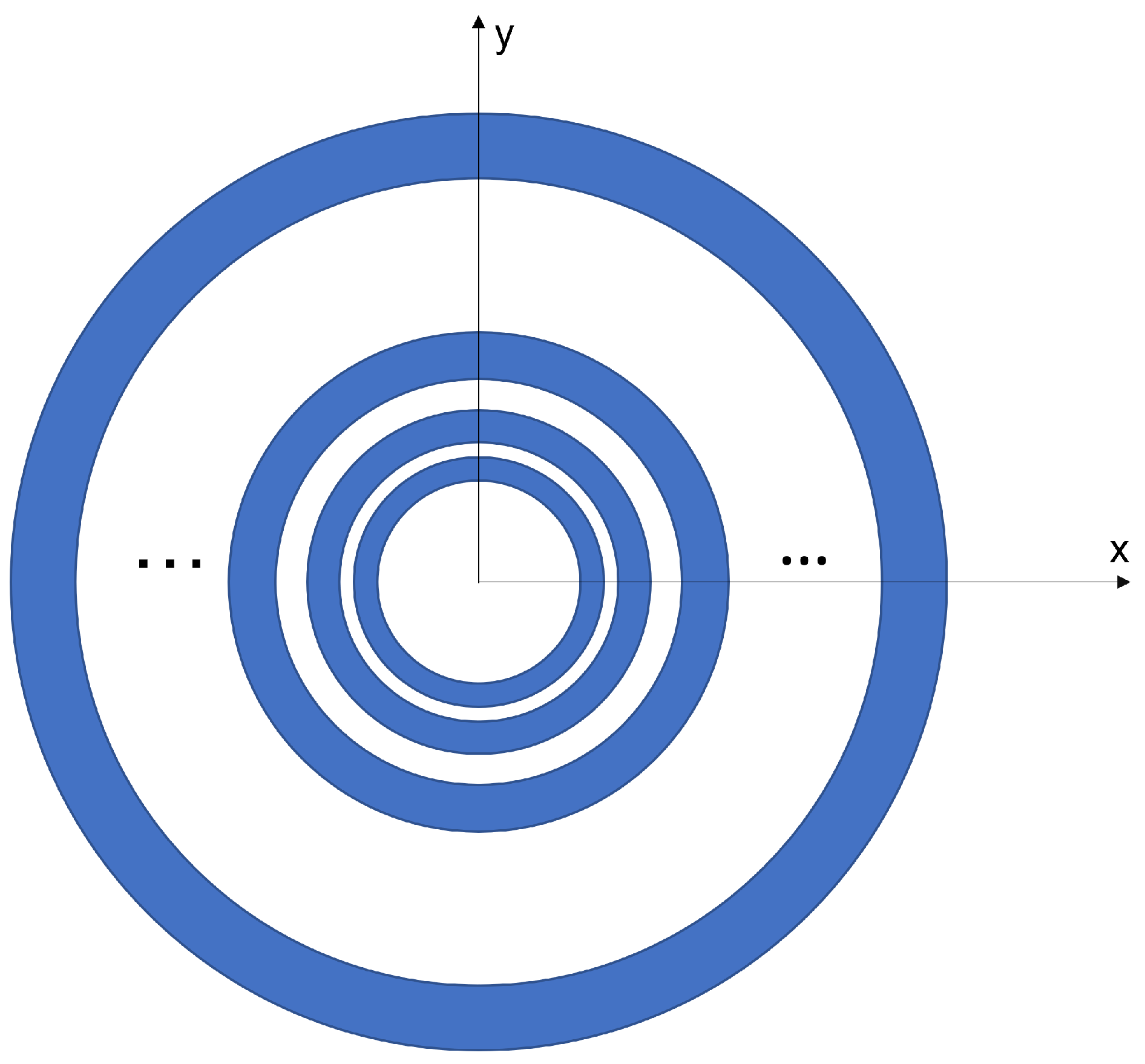
Let us consider the geometry depicted in Figure 1: a set of Q coplanar concentric rings, with inner and outer radii $r_{iq}$ and $r_{oq}$, respectively, for $q=1\dots Q$. A plane wave impinges on the rings with an incidence angle ${\theta }_{inc}$ with respect to z axis. Due to the symmetry the azimuthal angle of incidence is not essential and can be set to 0. Many different configurations are considered throughout the paper. All dimensions normalized to wavelength are summarized in

Table 1. List of configurations analyzed throughout the paper. All dimensions are normalized to the wavelength.

Label	${\mathit{r}}_{\mathit{i}1}$	${\mathit{r}}_{\mathit{o}1}$	${\mathit{r}}_{\mathit{i}2}$	${\mathit{r}}_{\mathit{o}2}$	${\mathit{r}}_{\mathit{i}3}$	${\mathit{r}}_{\mathit{o}3}$	${\mathit{r}}_{\mathit{i}4}$	${\mathit{r}}_{\mathit{o}4}$	${\mathit{r}}_{\mathit{i}5}$	${\mathit{r}}_{\mathit{o}5}$	${\mathit{r}}_{\mathit{i}6}$	${\mathit{r}}_{\mathit{o}6}$
Geom1	0.2	0.6	0.62	1.02	1.04	1.44	-	-	-	-	-	-
Geom2	0.2	0.4	0.6	0.8	1	1.2	1.4	1.6	-	-	-	-
Geom3	0.2	0.4	0.42	0.62	0.64	0.84	0.86	1.06	-	-	-	-
Geom4	0.2	0.25	0.3	0.35	0.4	0.45	0.5	0.55	0.6	0.65	0.7	0.75

. In particular, geometry #1 is composed of rings with a quite large width, very close to each other. In geometry #2, a regular lattice of four rings and slits is considered, whereas in geometry #3 the same rings as in geometry #2 are considered, but they are very close to each other. Finally, geometry #4 is again a regular lattice of rings and slits, with six narrow elements.

Due to the revolution symmetry of the geometry, a cylindrical harmonics expansion can be adopted for currents and fields. Moreover, the radial and azimuthal components will be gathered in vector notation as

$$\begin{array}{c}\hfill {\underline{F}}^{\left(n\right)}(\rho ,z)\equiv \underline{F}(\rho ,z)=\left[\begin{array}{c}{F}_r(\rho ,z)\\ -j{F}_{\phi }(\rho ,z)\end{array}\right]\end{array}$$

(1)

In (1) $\underline{F}$ represents the nth harmonic of either the surface current density or the field. Note that since cylindrical harmonics are independent of each other, the analysis can be carried out harmonic by harmonic. Consequently the superscript $\left(n\right)$ is understood and will be omitted throughout the paper. The VHT of $\underline{F}$ will also be introduced as

$$\begin{array}{c}\hfill \underline{\tilde{F}}(w,z)={\int }_0^{\infty }{\underline{\underline{H}}}_n\left(w\rho \right)\underline{F}(\rho ,z)\rho d\rho \end{array}$$

(2)

where the kernel of VHT is defined as

$$\begin{array}{c}\hfill {\underline{\underline{H}}}_n\left(w\rho \right)=\left[\begin{array}{cc}{J}_n^{\prime }\left(w\rho \right)& \frac{n}{w\rho }{J}_n\left(w\rho \right)\\ \frac{n}{w\rho }{J}_n\left(w\rho \right)& J_n^{\prime }\left(w\rho \right)\end{array}\right]\end{array}$$

(3)

$J_n(·)$ being the Bessel function of the first kind and order n and the apex representing the derivative with respect to the argument. Some useful properties of the VHT can be found in [46] whereas its relationship with the Scalar Hankel Transform is quite evident and will be employed later on.

The incident electromagnetic field induces a surface current on the rings, which in turn generates a scattered field. Such scattered field can then be written in the spectral domain as in [47], the generalization to multiple rings being straightforward

$$\begin{array}{c}\hfill {\underline{E}}_{sc}(\rho ,z)=j\frac{{\zeta }_0}{2}\sum _{q=1}^Q{\int }_0^{\infty }{\underline{\underline{H}}}_n\left(w\rho \right)\underline{\underline{G}}\left(w\right){\underline{\tilde{J}}}_q\left(w\right)e^{-j\left|z\right|\sqrt{k_0^2-w^2}}wdw\end{array}$$

(4)

where ${\zeta }_0$ and $k_0$ are the free space impedance and wavenumber, respectively. In (4) ${\underline{\tilde{J}}}_q\left(w\right)$ is the VHT of the current density induced on $q-th$ ring, and $\underline{\underline{G}}\left(w\right)$ is the Green’s function in the spectral domain, defined as

$$\begin{array}{c}\hfill \underline{\underline{G}}\left(w\right)=\left[\begin{array}{cc}{K}^{TM}\left(w\right)& 0\\ 0& K^{TE}\left(w\right)\end{array}\right]=\left[\begin{array}{cc}\frac{\sqrt{w^2-k_0^2}}{k_0}& 0\\ 0& -\frac{k_0}{\sqrt{w^2-k_0^2}}\end{array}\right]\end{array}$$

(5)

An Electric Field Integral Equation (EFIE) can then be obtained by imposing the boundary condition at $z=0$, that is the null of the tangential component of the total electric field, as

$$\begin{array}{c}\hfill {\underline{E}}_{sc}(\rho ,z=0)=-{\underline{E}}_{inc}(\rho ,z=0)\rho \in \bigcup _{q=1\cdots Q}[r_{iq},r_{oq}]\end{array}$$

(6)

Relation (6) represents a couple of IEs to be solved with respect to the unknown current densities. In the following subsections the proposed method will be described to achieve the analytical regularization of the problem at hand.

2.1. MoM Solution: Expansion

Equation (6) can be solved numerically by means of MoM. However, caution has to be paid when resorting to numerical methods, as their accuracy and effectiveness, or even their convergence, cannot be taken for granted at all. MAP can allow it to achieve all three mentioned attractive features, by applying a Galerkin discretization scheme, with a suitable selection of expansion and projection functions, to recast the integral equation as a Fredholm second-kind matrix operator equation. In particular, such an approach properly works, i.e., Fredholm theory can be applied, even when the most singular part of the obtained matrix operator is not diagonal but simply invertible with a continuous two-side inverse and the remaining part is a compact operator [26]. As a matter of fact, it has been shown that such a goal is achieved when using expansion functions factorizing the correct edge behavior of the unknowns in the spatial domain. Furthermore, in order for the method to also be effective, it is desirable to be able to perform the transform of the expansion functions analytically. All mentioned features can be found in the following functions:

$$\begin{array}{c}\hfill {\psi }_m\left(\rho \right)=\frac{4\rho p\left(\rho \right)}{\pi ab}{T}_n\left(\frac{{\rho }^2+r_i{r}_o}{2\rho a}\right)T_m\left(1-2\frac{{\rho }^2-r_i^2}{r_o^2-r_i^2}\right)with\rho \in [r_i,r_o]\end{array}$$

(7)

$$\begin{array}{c}\hfill {\chi }_m\left(\rho \right)=\frac{4\rho }{\pi p\left(\rho \right)ab}{T}_n\left(\frac{{\rho }^2+r_i{r}_o}{2\rho a}\right)T_m\left(1-2\frac{{\rho }^2-r_i^2}{r_o^2-r_i^2}\right)with\rho \in [r_i,r_o]\end{array}$$

(8)

where $T_h(·)$ is the Chebychev polynomial of first kind and order h, and the weighting function $p\left(\rho \right)=\sqrt{({\rho }^2-r_i^2)(r_o^2-{\rho }^2)}$ factorizes the correct edge behavior of the current components according to Meixner conditions [48]. Thus, (7) and (8) can be used as expansion functions of radial and azimuthal components of the induced current density, respectively, as shown later in expression (13). In particular, it is worth noting that in (7) and (8) the first Chebychev polynomial, which is a continuous, smooth, functional, and depends on the azimuthal index, but is independent of m and the weighting function $p\left(\rho \right)$. Consequently, when summing over m it is factorized and the reconstruction of the smooth part of the current density is left to the Chebychev polynomials of order m.

Furthermore, the Hankel transform of functions (7) and (8) is analytical; indeed, the scalar Hankel transform of ${\chi }_m\left(\rho \right)$ is known and can be written as [47]

$$\begin{array}{c}\hfill {\int }_{r_i}^{r_o}\rho {\chi }_m\left(\rho \right)J_n\left(w\rho \right)d\rho =J_{n+m}\left(wa\right)J_m\left(wb\right)\equiv F_m\left(w\right)\end{array}$$

(9)

where $a=(r_i+r_o)/2$ and $b=(r_o-r_i)/2$. Since ${\chi }_m\left(\rho \right)$ is suitable as an expansion function of the azimuthal component of the current density, resembling notation (1), we can consider the quantity $\left[\begin{array}{c}0\\ {\chi }_m\left(\rho \right)\end{array}\right]$, for which it is easy to show that

$$\begin{array}{c}\hfill VHT\left[\begin{array}{c}0\\ {\chi }_m\left(\rho \right)\end{array}\right]=\left[\begin{array}{c}\frac{n}{w}\\ \frac{d}{dw}\end{array}\right]F_m\left(w\right)\end{array}$$

(10)

Moreover, using the recurrence relations of Chebychev polynomials, after some algebraic manipulations it is possible to demonstrate the following recurrence relationship

$$\begin{array}{c}\hfill {\int }_{r_i}^{r_o}\rho {\psi }_m\left(\rho \right)J_n\left(w\rho \right)d\rho =2F_m\left(w\right)-F_{m-2}\left(w\right)-F_{m+2}\left(w\right)\equiv G_m\left(w\right)\end{array}$$

(11)

which also defines the scalar Hankel transform of ${\psi }_m\left(\rho \right)$. Similar to what was conducted before, we can consider the quantity $\left[\begin{array}{c}{\psi }_m\left(\rho \right)\\ 0\end{array}\right]$ and calculate the corresponding VHT as

$$\begin{array}{c}\hfill VHT\left[\begin{array}{c}{\psi }_m\left(\rho \right)\\ 0\end{array}\right]=\left[\begin{array}{c}\frac{d}{dw}\\ \frac{n}{w}\end{array}\right]G_m\left(w\right)\end{array}$$

(12)

Finally, it is worth noting that recurrence relation (11) can be very helpful in the evaluation of the scattering matrix in order to reduce the overall number of integrals to be calculated numerically.

Consequently, the unknown current density can be expanded as

$$\begin{array}{cc}\hfill \underline{J}\left(\rho \right)=& \sum _{q=1}^Q\sum _{m=0}^{\infty }\left\{c_m^{\left(q\right)}\left[\begin{array}{c}{\psi }_m^{\left(q\right)}\left(\rho \right)\\ 0\end{array}\right]+d_m^{\left(q\right)}\left[\begin{array}{c}0\\ {\chi }_m^{\left(q\right)}\left(\rho \right)\end{array}\right]\right\}\hfill \\ \hfill =& \sum _{q=1}^Q\sum _{m=0}^{\infty }\left\{c_m^{\left(q\right)}{\underline{\Psi }}_m^{\left(q\right)}\left(\rho \right)+d_m^{\left(q\right)}{\underline{X}}_m^{\left(q\right)}\left(\rho \right)\right\}\hfill \end{array}$$

(13)

where $c_m^{\left(q\right)}$ and $d_m^{\left(q\right)}$ are unknown expansion coefficients to be evaluated numerically. Its VHT can be calculated analytically as shown above, and can be substituted into the scattered field, to give the integral equation

$$\begin{array}{c}\hfill j\frac{{\zeta }_0}{2}\sum _{q=1}^Q\sum _{m=0}^{\infty }{\int }_0^{\infty }{\underline{\underline{H}}}_n\left(w\rho \right)\underline{\underline{G}}\left(w\right)\left\{c_m^{\left(q\right)}\left[\begin{array}{c}\frac{d}{dw}\\ \frac{n}{w}\end{array}\right]G_m\left(w\right)+d_m^{\left(q\right)}\left[\begin{array}{c}\frac{n}{w}\\ \frac{d}{dw}\end{array}\right]F_m\left(w\right)\right\}wdw=\\ \hfill -{\underline{E}}_{inc}(\rho ,z=0)\end{array}$$

(14)

In the following subsection the next step of the procedure will be described, leading to the solution of the problem.

2.2. MoM Solution: Projection

Equation (14) can be solved by means of a suitable projection: in order to fall in the framework of Galerkin’s Method, we can multiply both sides of the equation by ${\left[{\underline{\Psi }}_m^{\left(p\right)}\left(\rho \right)\right]}^T$ and ${\left[{\underline{X}}_m^{\left(p\right)}\left(\rho \right)\right]}^T$ with $p=1\dots Q$, where the superscript T stands for transpose, and integrate with respect to $\rho d\rho$ from $r_{ip}$ to $r_{op}$. Such a projection is analytical on both sides of the equation; on the left hand side it is just necessary to apply again the VHT Formulas (10) and (12), whereas on the right hand side, resorting to the cylindrical wave expansion of a plane wave, it is not difficult to show that

$$\begin{array}{c}\hfill {\int }_{r_{ip}}^{r_{op}}{\left[{\underline{\Psi }}_m^{\left(p\right)}\left(\rho \right)\right]}^T{\underline{E}}_{inc}(\rho ,z=0)\rho d\rho =j^{n-1}\frac{n}{k_{0}sin{\vartheta }_i}{F}_k^{\left(p\right)}\left(k_{0}sin{\vartheta }_i\right)\end{array}$$

(15)

$$\begin{array}{c}\hfill {\int }_{r_{ip}}^{r_{op}}{\left[{\underline{X}}_m^{\left(p\right)}\left(\rho \right)\right]}^T{\underline{E}}_{inc}(\rho ,z=0)\rho d\rho =j^{n-1}\frac{d{G}_k^{\left(p\right)}\left(w\right)}{dw}{|}_{k_{0}sin{\vartheta }_i}\end{array}$$

(16)

in the Transverse Magnetic (TM) case, and

$$\begin{array}{c}\hfill {\int }_{r_{ip}}^{r_{op}}{\left[{\underline{\Psi }}_m^{\left(p\right)}\left(\rho \right)\right]}^T{\underline{E}}_{inc}(\rho ,z=0)\rho d\rho =j^{n-1}\frac{d{F}_k^{\left(p\right)}\left(w\right)}{dw}{|}_{k_{0}sin{\vartheta }_i}\end{array}$$

(17)

$$\begin{array}{c}\hfill {\int }_{r_{ip}}^{r_{op}}{\left[{\underline{X}}_m^{\left(p\right)}\left(\rho \right)\right]}^T{\underline{E}}_{inc}(\rho ,z=0)\rho d\rho =j^{n-1}\frac{n}{k_{0}sin{\vartheta }_i}{G}_k^{\left(p\right)}\left(k_{0}sin{\vartheta }_i\right)\end{array}$$

(18)

in the Transverse Electric (TE) case. The problem is therefore reduced to the solution of an algebraic system of linear equations. The coefficients’ matrix, that is the scattering matrix, has to be computed numerically. This is not generally an easy task, as the entries of the matrix are integrals of slowly decaying oscillating functions. Different strategies can be adopted to accelerate the numerical computation of the integrals. A first possibility is to subtract the asymptotic behavior of the kernels, thus leading to integrals of the product of four Bessel functions and powers. Such an approach has been used, for example, in [44] in a simpler, scalar case. As a matter of fact, it can be shown that the integral of the product of four Bessel functions can be analytically evaluated as a Meijer function. This is very useful for numerical calculation because currently there are efficient routines evaluating such a special function.

A second possible approach consists of resorting to the integration in the complex plane along a suitable integration path, as performed in [47]. In such a case the integrals at hand can be written as a superposition of proper integrals and fast converging improper integrals. In both cases, an effective calculation of the scattering matrix is possible, and numerical results can be obtained without excessive computational burden.

3. Results

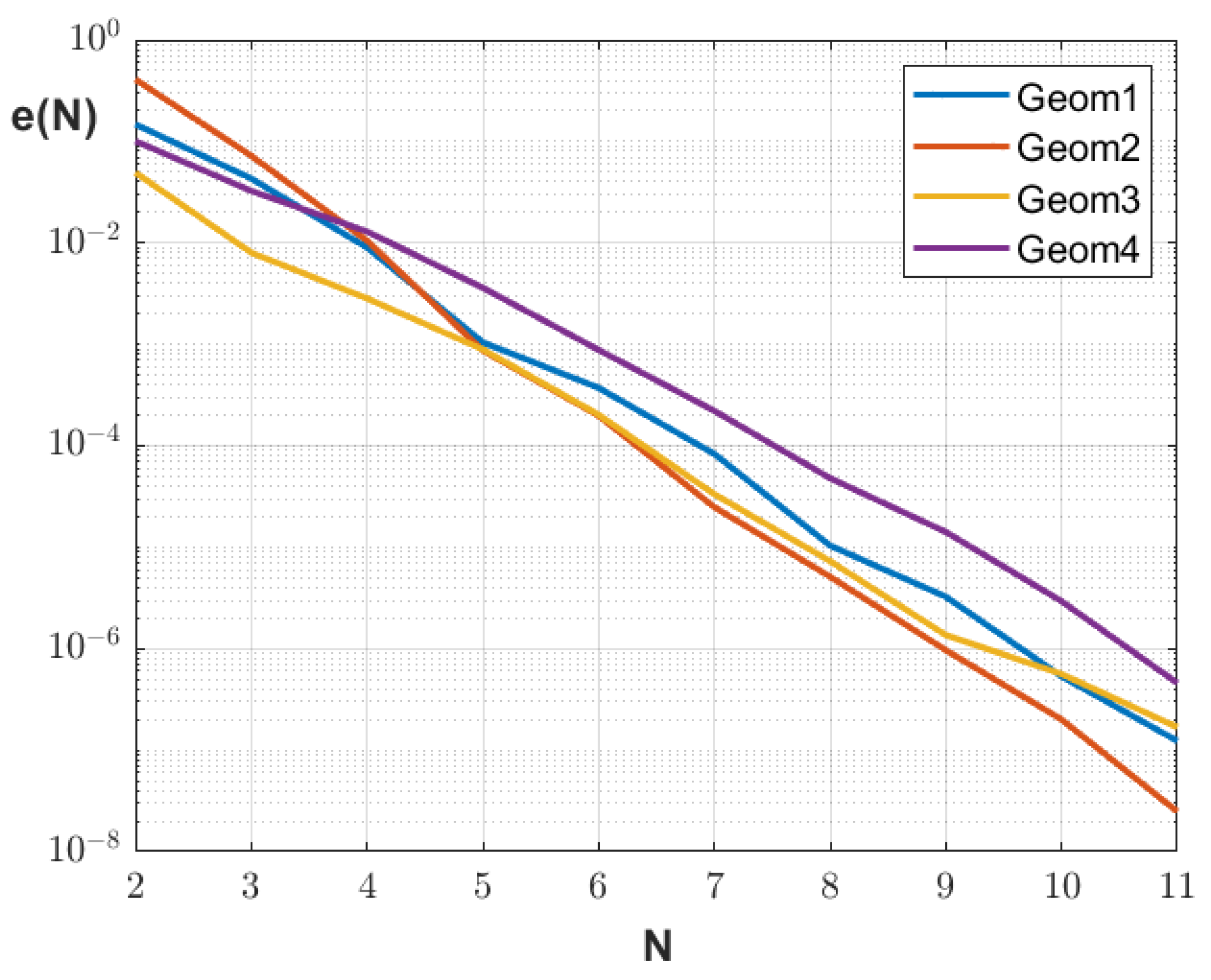
As a first task, the convergence of the method has been checked. As outlined in the Introduction, a blind application of numerical methods can lead to slow convergence, or could even not converge at all. On the contrary MAR allows to achieve fast convergence and error control. In order to verify the effectiveness of the method illustrated in previous Section the following error is introduced

$$\begin{array}{c}\hfill e\left(N\right)=\frac{∥{\mathbf{c}}^{(\mathbf{N}+\mathbf{1})}-{\mathbf{c}}^{\left(\mathbf{N}\right)}∥}{∥{\mathbf{c}}^{\left(\mathbf{N}\right)}∥}+\frac{∥{\mathbf{d}}^{(\mathbf{N}+\mathbf{1})}-{\mathbf{d}}^{\left(\mathbf{N}\right)}∥}{∥{\mathbf{d}}^{\left(\mathbf{N}\right)}∥}\end{array}$$

(19)

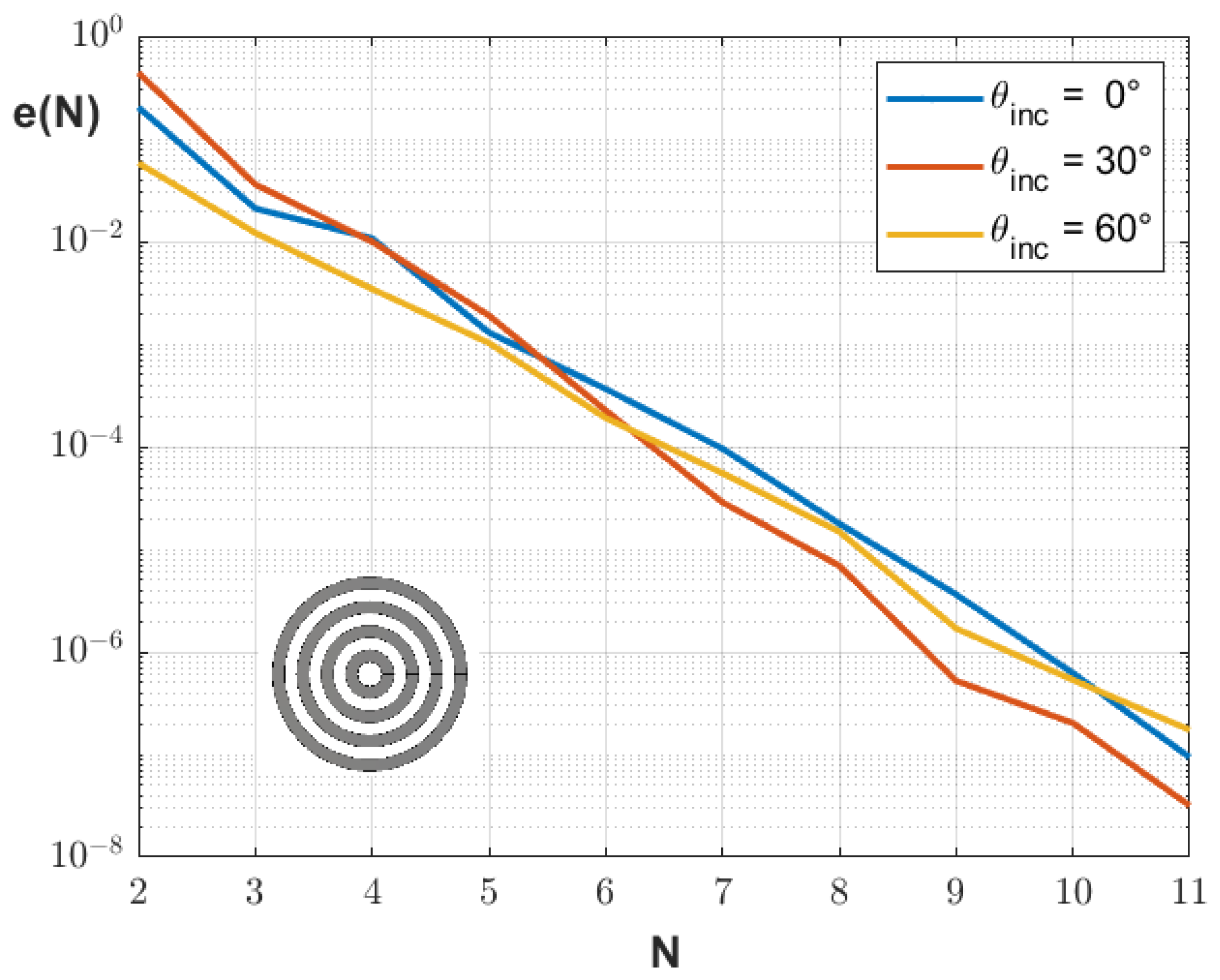
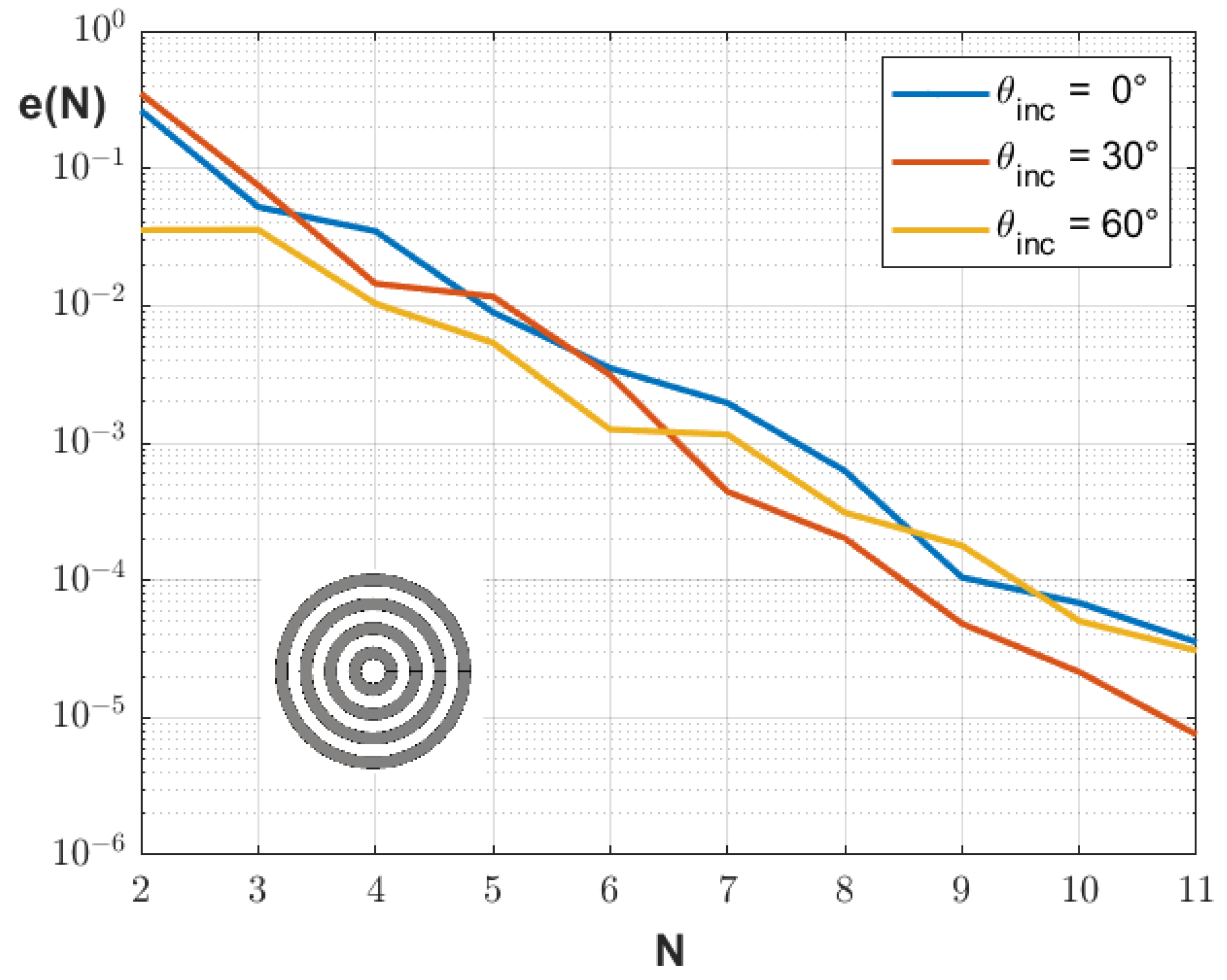
where N is the truncation order (actually, two different truncation orders should be introduced for the two components of the current. In the present work they have been taken equal for simplicity), namely the number of terms retained in expansion (13.), ${\mathbf{c}}^{\left(\mathbf{N}\right)}$ and ${\mathbf{d}}^{\left(\mathbf{N}\right)}$ are the coefficients vectors corresponding to that truncation error, and the standard euclidean norm in ${\ell }^2$ is employed. The error is plotted in Figure 2 for all geometries listed in Table 1 in TE case for an incidence angle ${\theta }_{inc}=45$. In Figure 3 and Figure 4 the error is plotted for geometry #2, for different incidence angles, in TE and TM case, respectively. As can be seen, in all the cases shown, as well as in any other case considered and not displayed for the sake of brevity, the error is exponentially decaying, thus confirming the effectiveness of the method. In the following all the reported examples have been calculated taking into account seven expansion terms, thus ensuring an accuracy not larger than ${10}^{-3}$.

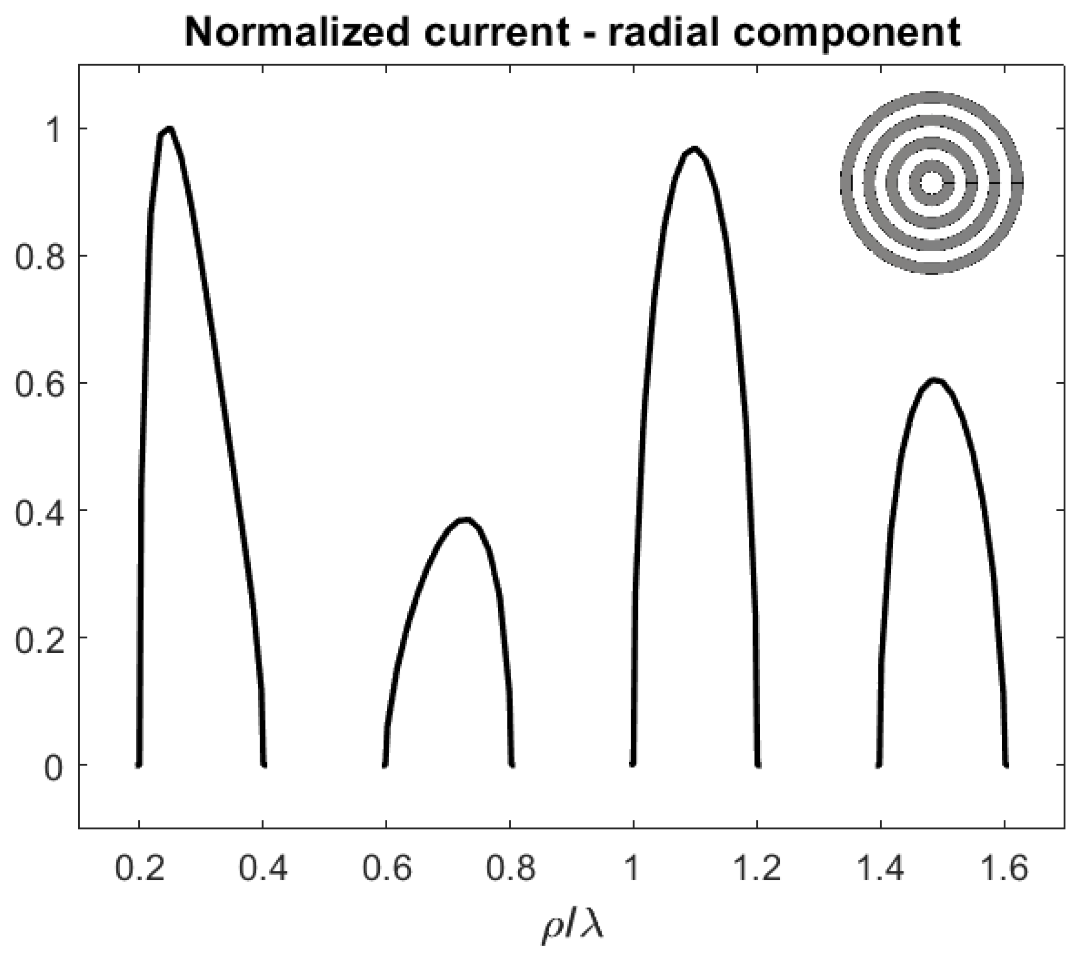
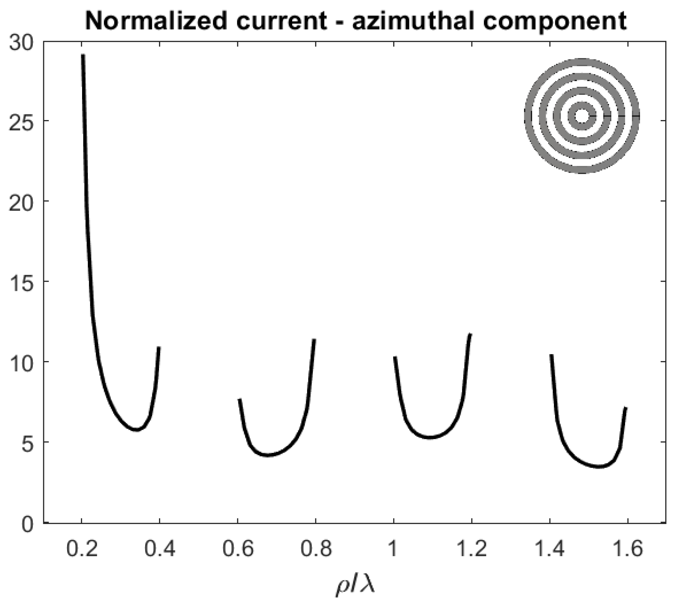
Once the unknown coefficients have been calculated, the currents and the fields can be evaluated. As an example, the reconstructed current density behavior is plotted in Figure 5 and Figure 6 for the case of geometry #2 of Table 1 for an incidence angle ${\theta }_{inc}=0$. As can be seen, the edge behavior of both current components is perfectly reconstructed. As expected, the radial component vanishes at the edges, whereas the azimuthal component diverges, as prescribed by Meixner’s conditions [48].

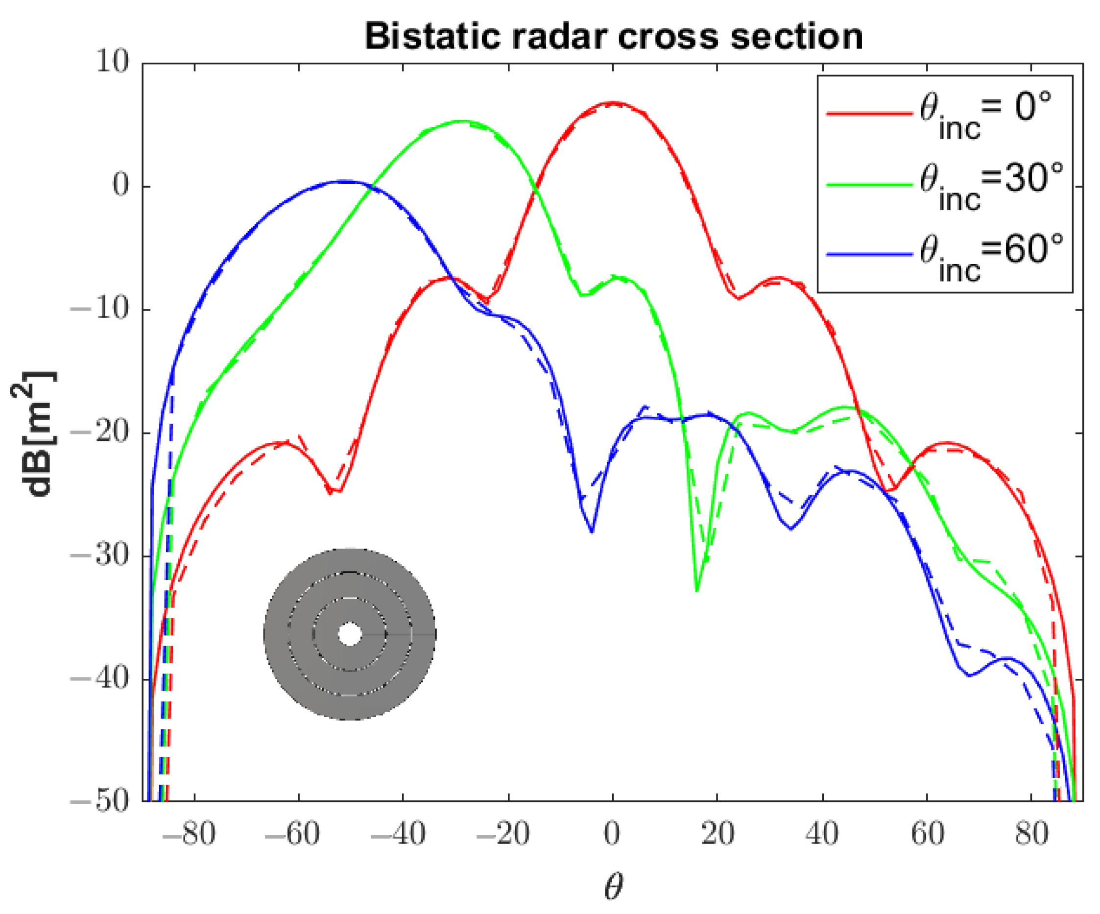
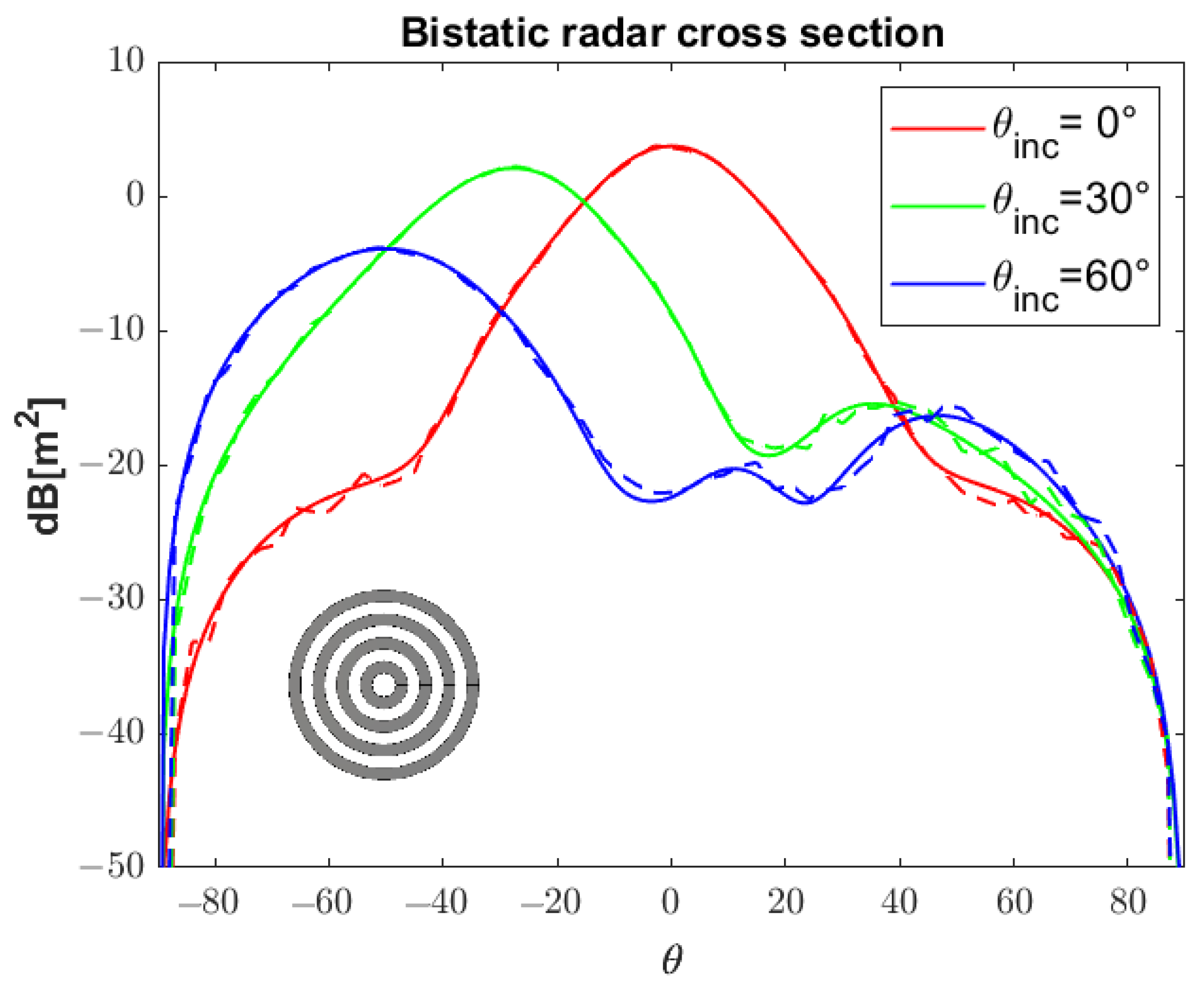
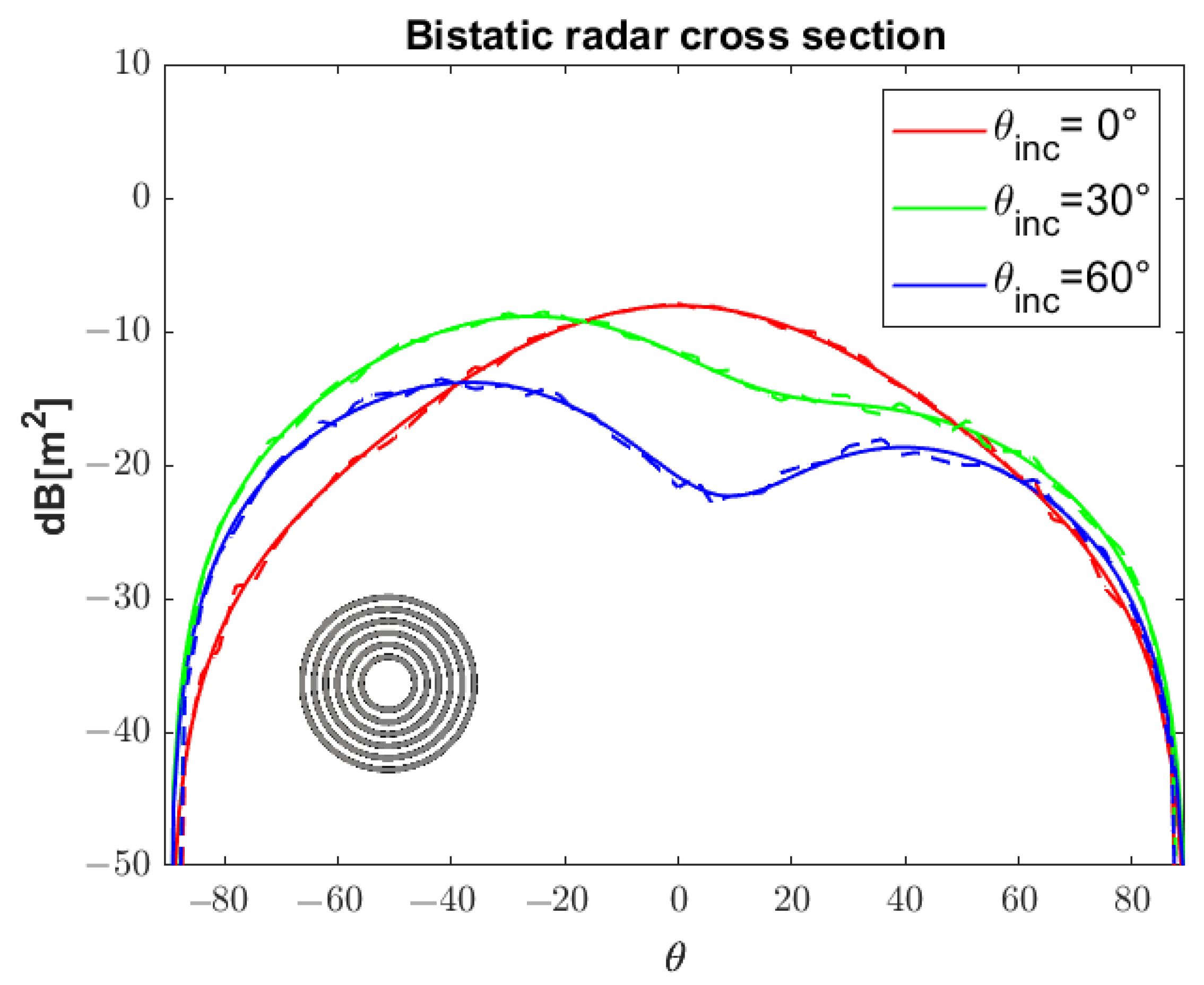
Finally, the bistatic radar cross section is plotted in Figure 7, Figure 8 and Figure 9 for different geometries and different incidence angles. As expected, the more oblique the incidence, the less smooth the radar cross section. In the same plots, a comparison with CST Microwave Studio is also shown, exhibiting a very good agreement in any case.

4. Conclusions

In this paper, a method for the analysis of infinitesimally thin coupled perfectly conducting rings has been presented. The procedure falls within the framework of Analytical Regularization, i.e., methods which converge to the solution and allow the full control of the discretization error when the number of ’mesh points’ is increased. The proposed methodology is based on a suitable choice of the functions to be used in a Galerkin’s scheme, which factorize the correct edge behavior of the unknowns. The method proved itself to be very accurate and fast converging in all the considered examples. Only coplanar rings in free space have been considered in this work, in order to focus on the method itself, but the generalization to stratified media is straightforward, with a suitable change of the Green’s function of the problem at hand. Furthermore, a change of the incident field does not impact on the method and on the calculation of the scattering matrix. The method can then be applied to the many different contexts, as mentioned in the Introduction.

References

- Chew, W. A broad-band annular-ring microstrip antenna. IEEE Trans. Antennas Propag. 1982, 30, 918–922. [Google Scholar] [CrossRef]
- Dahele, J.; Lee, K.F.; Wong, D. Dual-frequency stacked annular-ring microstrip antenna. IEEE Trans. Antennas Propag. 1987, 35, 1281–1285. [Google Scholar] [CrossRef]
- Tong, K.F.; Huang, J. New proximity coupled feeding method for reconfigurable circularly polarized microstrip ring antennas. IEEE Trans. Antennas Propag. 2008, 56, 1860–1866. [Google Scholar] [CrossRef]
- Guo, Y.X.; Bian, L.; Shi, X.Q. Broadband circularly polarized annular-ring microstrip antenna. IEEE Trans. Antennas Propag. 2009, 57, 2474–2477. [Google Scholar]
- Zhang, Y.Q.; Li, X.; Yang, L.; Gong, S.X. Dual-band circularly polarized annular-ring microstrip antenna for GNSS applications. IEEE Antennas Wirel. Propag. Lett. 2013, 12, 615–618. [Google Scholar] [CrossRef]
- Munde, M.; Nandgaonkar, A.; Deosarkar, S. Dual feed wideband annular ring microstrip antenna with circular DGS for reduced SAR. Prog. Electromagn. Res. B 2020, 88, 175–195. [Google Scholar] [CrossRef]
- Ramirez, M.; Parrón, J.; Gonzalez-Arbesu, J.M.; Gemio, J. Concentric annular-ring microstrip antenna with circular polarization. IEEE Antennas Wirel. Propag. Lett. 2011, 10, 517–519. [Google Scholar] [CrossRef]
- Bhattacharyya, A.; Garg, R. A microstrip array of concentric annular rings. IEEE Trans. Antennas Propag. 1985, 33, 655–659. [Google Scholar] [CrossRef]
- Kanaujia, B.K.; Vishvakarma, B.R. Analysis of two-concentric annular ring microstrip antenna. Microw. Opt. Technol. Lett. 2003, 36, 104–108. [Google Scholar] [CrossRef]
- Bao, X.; Ammann, M. Compact concentric annular-ring patch antenna for triple-frequency operation. Electron. Lett. 2006, 42, 1129–1130. [Google Scholar] [CrossRef] [Green Version]
- Luo, S.; Thorburn, M.; Tripathi, V. Modelling of multiple coupled concentric open and closed microstrip ring structure. IEE Proc. Microwaves Antennas Propag. 1991, 138, 573–576. [Google Scholar] [CrossRef]
- Prasad, G.R.; Madhav, B.; Pardhasaradhi, P.; Devi, Y.U.; Nadh, B.P.; Anilkumar, T.; Rao, M.V. Concentric Ring Structured Reconfigurable Antenna using MEMS Switches for Wireless Communication Applications. Wirel. Pers. Commun. 2021, 120, 587–608. [Google Scholar] [CrossRef]
- Orefice, M.; Pirinoli, P.; Drocco, A. Analysis of complex circular/square ring reflectarray elements. In Proceedings of the 2009 IEEE 3rd European Conference on Antennas and Propagation, Berlin, Germany, 23–27 March 2009; pp. 1357–1359. [Google Scholar]
- Wu, T. Frequency Selective Surface and Grid Array; Wiley: New York, NY, USA, 1995. [Google Scholar]
- Taylor, P.S.; Parker, E.A.; Batchelor, J.C. An active annular ring frequency selective surface. IEEE Trans. Antennas Propag. 2011, 59, 3265–3271. [Google Scholar] [CrossRef] [Green Version]
- Jin, C.; Lv, Q.; Mittra, R. Dual-polarized frequency-selective surface with two transmission zeros based on cascaded ground apertured annular ring resonators. IEEE Trans. Antennas Propag. 2018, 66, 4077–4085. [Google Scholar] [CrossRef]
- Delyser, R.R.; Chang, D.C.; Kuester, E.F. Design of a log periodic strip grating microstrip antenna. Int. J. Microw. Millimeter-Wave Comput.-Aided Eng. 1993, 3, 143–150. [Google Scholar] [CrossRef]
- Podilchak, S.K.; Baccarelli, P.; Burghignoli, P.; Freundorfer, A.P.; Antar, Y.M. Analysis and design of annular microstrip-based planar periodic leaky-wave antennas. IEEE Trans. Antennas Propag. 2014, 62, 2978–2991. [Google Scholar] [CrossRef]
- Wang, D.; Yang, T.; Crozier, K.B. Optical antennas integrated with concentric ring gratings: Electric field enhancement and directional radiation. Opt. Express 2011, 19, 2148–2157. [Google Scholar] [CrossRef]
- Chen, F.; Wang, S.W.; Zhang, Y.; Li, Q.; Sun, X.; Chen, X.; Lu, W. Simulation of superconducting single photon detector coupled with metal–insulator–metal concentric ring grating. Opt. Quantum Electron. 2014, 46, 1253–1259. [Google Scholar] [CrossRef]
- Feng, S.; Darmawi, S.; Henning, T.; Klar, P.J.; Zhang, X. A miniaturized sensor consisting of concentric metallic nanorings on the end facet of an optical fiber. Small 2012, 8, 1937–1944. [Google Scholar] [CrossRef]
- Kolton, D.; Kress, R. Inverse Acoustic and Electromagnetic Scattering Theory; Springer: Berlin, Germany, 2013; Volume 93. [Google Scholar]
- Dudley, D. Error minimization and convergence in numerical methods. Electromagnetics 1985, 5, 89–97. [Google Scholar] [CrossRef]
- Nosich, A.I. The method of analytical regularization in wave-scattering and eigenvalue problems: Foundations and review of solutions. IEEE Antennas Propag. Mag. 1999, 41, 34–49. [Google Scholar] [CrossRef]
- Fikioris, G. A note on the method of analytical regularization. IEEE Antennas Propag. Mag. 2001, 43, 34–40. [Google Scholar] [CrossRef]
- Kantorovich, L.V.; Akilov, G.P. Functional Analysis, 2nd ed.; Pergamon Press: Oxford, UK, 1982. [Google Scholar]
- Nosich, A.I. Method of analytical regularization in computational photonics. Radio Sci. 2016, 51, 1421–1430. [Google Scholar] [CrossRef]
- Veliev, E.; Veremay, V. Numerical-analytical approach for the solution to the wave scattering by polygonal cylinders and flat strip structures. In Analytical and Numerical Methods in Electromagnetic Wave Theory; Science House: Tokyo, Japan, 1993; Volume 10. [Google Scholar]
- Hongo, K.; Serizawa, H. Diffraction of electromagnetic plane wave by a rectangular plate and a rectangular hole in the conducting plate. IEEE Trans. Antennas Propag. 1999, 47, 1029–1041. [Google Scholar] [CrossRef]
- Losada, V.; Boix, R.R.; Horno, M. Full-wave analysis of circular microstrip resonators in multilayered media containing uniaxial anisotropic dielectrics, magnetized ferrites, and chiral materials. IEEE Trans. Microw. Theory Tech. 2000, 48, 1057–1064. [Google Scholar] [CrossRef] [Green Version]
- Tsalamengas, J. Rapidly converging direct singular integral-equation techniques in the analysis of open microstrip lines on layered substrates. IEEE Trans. Microw. Theory Tech. 2001, 49, 555–559. [Google Scholar] [CrossRef]
- Lucido, M.; Panariello, G.; Schettino, F. TE scattering by arbitrarily connected conducting strips. IEEE Trans. Antennas Propag. 2009, 57, 2212–2216. [Google Scholar] [CrossRef]
- Coluccini, G.; Lucido, M.; Panariello, G. TM scattering by perfectly conducting polygonal cross-section cylinders: A new surface current density expansion retaining up to the second-order edge behavior. IEEE Trans. Antennas Propag. 2011, 60, 407–412. [Google Scholar] [CrossRef]
- Coluccini, G.; Lucido, M.; Panariello, G. Spectral domain analysis of open single and coupled microstrip lines with polygonal cross-section in bound and leaky regimes. IEEE Trans. Microw. Theory Tech. 2012, 61, 736–745. [Google Scholar] [CrossRef]
- Coluccini, G.; Lucido, M. A new high efficient analysis of the scattering by a perfectly conducting rectangular plate. IEEE Trans. Antennas Propag. 2013, 61, 2615–2622. [Google Scholar] [CrossRef]
- Lucido, M. Electromagnetic scattering by a perfectly conducting rectangular plate buried in a lossy half-space. IEEE Trans. Geosci. Remote Sens. 2014, 52, 6368–6378. [Google Scholar] [CrossRef]
- Di Murro, F.; Lucido, M.; Panariello, G.; Schettino, F. Guaranteed-convergence method of analysis of the scattering by an arbitrarily oriented zero-thickness PEC disk buried in a lossy half-space. IEEE Trans. Antennas Propag. 2015, 63, 3610–3620. [Google Scholar] [CrossRef]
- Lucido, M.; Migliore, M.D.; Pinchera, D. A new analytically regularizing method for the analysis of the scattering by a hollow finite-length PEC circular cylinder. Prog. Electromagn. Res. 2016, 70, 55–71. [Google Scholar] [CrossRef] [Green Version]
- Lucido, M.; Panariello, G.; Schettino, F. Scattering by a zero-thickness PEC disk: A new analytically regularizing procedure based on Helmholtz decomposition and Galerkin method. Radio Sci. 2017, 52, 2–14. [Google Scholar] [CrossRef]
- Lovat, G.; Burghignoli, P.; Araneo, R.; Celozzi, S.; Andreotti, A.; Assante, D.; Verolino, L. Shielding of a perfectly conducting circular disk: Exact and static analytical solution. Prog. Electromagn. Res. 2019, 95, 167–182. [Google Scholar] [CrossRef] [Green Version]
- Lucido, M.; Schettino, F.; Panariello, G. Scattering from a thin resistive disk: A guaranteed fast convergence technique. IEEE Trans. Antennas Propag. 2020, 69, 387–396. [Google Scholar] [CrossRef]
- Yevtushenko, F.O.; Dukhopelnykov, S.V.; Nosich, A.I. H-polarized plane-wave scattering by a PEC strip grating on top of a dielectric substrate: Analytical regularization based on the Riemann-Hilbert Problem solution. J. Electromagn. Waves Appl. 2020, 34, 483–499. [Google Scholar] [CrossRef]
- Assante, D.; Panariello, G.; Schettino, F.; Verolino, L. Coupling impedance of a PEC angular strip in a vacuum pipe. IET Microwaves Antennas Propag. 2021, 15, 1347–1359. [Google Scholar] [CrossRef]
- Assante, D.; Panariello, G.; Schettino, F.; Verolino, L. Longitudinal coupling impedance of a particle traveling in PEC rings: A regularised analysis. IET Microwaves Antennas Propag. 2021, 15, 1318–1329. [Google Scholar] [CrossRef]
- Assante, D.; Panariello, G.; Schettino, F.; Verolino, L. Analytically Regularized Evaluation of the Wakefield of a Particle Travelling through a Plane Conducting Ring. In Proceedings of the 2022 Microwave Mediterranean Symposium (MMS), Pizzo Calabro, Italy, 11–12 May 2022; pp. 1–5. [Google Scholar]
- Chew, W.; Kong, J. Resonance of nonaxial symmetric modes in circular microstrip disk antenna. J. Math. Phys. 1980, 21, 2590–2598. [Google Scholar] [CrossRef]
- Lucido, M.; Schettino, F.; Migliore, M.D.; Pinchera, D.; Di Murro, F.; Panariello, G. Electromagnetic scattering by a zero-thickness PEC annular ring: A new highly efficient MoM solution. J. Electromagn. Waves Appl. 2017, 31, 405–416. [Google Scholar] [CrossRef]
- Meixner, J. The behavior of electromagnetic fields at edges. IEEE Trans. Antennas Propag. 1972, 20, 442–446. [Google Scholar] [CrossRef]
Figure 1.
Geometry of the problem: Q coplanar perfectly conducting concentric rings, with inner and outer radii and , respectively, for . A plane wave impinges on the rings with an incidence angle with respect to z axis. Due to the symmetry the azimuthal angle of incidence is not essential.
Figure 2.
Plot of the error for the geometries of Table 1 for TE incidence and an incidence angle .
Figure 3.
Plot of the error for the geometry #2 of Table 1 (sketched in the inset) for TE incidence and different incidence angles .
Figure 4.
Plot of the error for the geometry #2 of Table 1 (sketched in the inset) for TM incidence and different incidence angles .
Figure 5.
Behavior of the radial component of the current density for the geometry #2 of Table 1 (sketched in the inset) for an incidence angle .
Figure 6.
Behavior of the azimuthal component of the current density for the geometry #2 of Table 1 (sketched in the inset) for an incidence angle .
Figure 7.
Bistatic radar cross section for geometry #1 (sketched in the inset) for different incidence angles . Solid line: this method; dashed line: CST Microwave Studio.
Figure 8.
Bistatic radar cross section for geometry #2 (sketched in the inset) for different incidence angles . Solid line: this method; dashed line: CST Microwave Studio.
Figure 9.
Bistatic radar cross section for geometry #4 (sketched in the inset) for different incidence angles . Solid line: this method; dashed line: CST Microwave Studio.