
Feature Drift in Fake News Detection: An Interpretable Analysis
by
Chenbo Fu
1,2,*,
Xingyu Pan
1,2,
Xuejiao Liang
1,2,
Shanqing Yu
1,2,
Xiaoke Xu
3 and
Yong Min
3,* 1
Institute of Cyberspace Security, Zhejiang University of Technology, Hangzhou 310023, China
2
College of Information Engineering, Zhejiang University of Technology, Hangzhou 310023, China
3
Computational Communication Research Center, Beijing Normal University, Zhuhai 519087, China
*
Authors to whom correspondence should be addressed.
Appl. Sci. 2023, 13(1), 592; https://0-doi-org.brum.beds.ac.uk/10.3390/app13010592
Submission received: 29 November 2022
/
Revised: 21 December 2022
/
Accepted: 28 December 2022
/
Published: 1 January 2023
(This article belongs to the Special Issue Advances in Big Data and Machine Learning)
Abstract
:In recent years, fake news detection and its characteristics have attracted a number of researchers. However, most detection algorithms are driven by data rather than theories, which causes the existing approaches to only perform well on specific datasets. To the extreme, several features only perform well on specific datasets. In this study, we first define the feature drift in fake news detection methods, and then demonstrate the existence of feature drift and use interpretable models (i.e., Shapley Additive Explanations and Partial Dependency Plots) to verify the feature drift. Furthermore, by controlling the distribution of tweets’ creation times, a novel sampling method is proposed to explain the reason for feature drift. Finally, the Anchors method is used in this paper as a supplementary interpretation to exhibit the potential characteristics of feature drift further. Our work provides deep insights into the temporal patterns of fake news detection, proving that the model’s performance is also highly related to the distribution of datasets.
1. Introduction
Social media have significantly increased the amount of information on the Internet due to their characteristics of fast information spreading and strong user mobility [1,2,3]. Meanwhile, the low-cost posting and spreading of ambiguous or misleading information on social media has significantly increased the probability of users to be exposed to fake news [4]. The rise of fake news affects information credibility in the era of high information technology [5]. Recent studies show that fake news has become one of the largest threats to democracy [6] and public opinion [7]. For example, it affected the “Brexit” referendum [8] and the 2016 US presidential election [9], resulting in the weak credibility of the government. Furthermore, it can be found that fake news is retweeted more often than genuine news [10,11].
Although fake news is not a new phenomenon, the rapidly changing social realities have prompted us to revisit the scientific theories and continue to develop new approaches to manage and analyze fake news, e.g., the systematic change in news consumption. Compared with traditional news media, such as newspapers and television, fake news is published and propagated online, faster and at a lower cost [12]. However, for the general public, the ability to identify fake news is very low [13]. Furthermore, the echo chamber effect on social media also amplifies and reinforces the spread of fake news [14], causing fake news to experience a high degree of exposure and a validity effect [15]. Thus, nowadays, detecting fake news has become extremely difficult.
Researchers have suggested various methods to study the propagation of fake news. Guess et al. [16] found that there is a strong age effect in fake news dissemination on social networks; users aged over sixty-five shared more fake news than younger users. Tsfati et al. [17] proposed that mainstream news media in fact play a significant and important role in the dissemination of fake news, which defies our intuitions. Kucharski [18] proposed a spreading dynamics model based on modified epidemic diffusion models to study the propagation of fake news. Ref. [14] proposed that echo chambers on social networks lead to the virality of fake news from the perspective of social contagion. In addition, researchers also suggest various algorithms to develop fake news detection methods based on machine learning [19,20] or deep learning [21,22,23,24]. However, their feature recognition work is driven by data rather than theories [25], which causes the existing approaches to only perform well on specific datasets. Furthermore, most current works focus on the linguistic features [26,27,28], which may be deliberately intended for specific purposes, e.g., deceptive language features can be injected to bypass the text-based rumor detection model [29]. Thus, the fragility of linguistic features prompts researchers to start looking for more reliable features, e.g., propagation features (such as propagation range, i.e., the size of the retweet network). Compared to linguistic features, they are more difficult to manipulate by malicious users [30]. Therefore, propagation-based methods [31,32,33] have more stable temporal and inter-system validity. However, the basic propagation characteristics and underlying mechanisms of user activity on social media platforms remain poorly understood.
In general, different data sources may introduce system biases and yield a lack of stability in the measurement. Thus, exploring underlying mechanisms in fake news detection becomes necessary. Furthermore, the interpretability of deep learning approaches is very poor, e.g., deep neural networks (DNN) [34]. These models, with low interpretability, are challenging to put into practical application, despite the high accuracy that they obtain. Our study demonstrates that the same features perform differently in different datasets. By defining the phenomenon of feature drift in fake news detection as the fact that the features are unstable and fortuitous over a decision process, our work proves the existence of feature drift and discusses the potential reasons. The research questions are as follows:
- RQ1: Does the phenomenon of feature drift exist in fake news detection?
- RQ2: What causes the feature drift phenomenon?
By using SHAP (Shapley Additive Explanations) [35] and PDP (Partial Dependency Plots) [36], we confirm the existence of the feature drift phenomenon. Furthermore, to identify the reason for feature drift, our work proposes a sampling method by controlling the distribution of tweets’ creation times. The contributions of this work are as follows:
- We demonstrate that the feature drift phenomenon does exist in fake news detection, and explainable results further illustrate the existence of feature drift.
- We propose a sampling method based on skewness to discuss the reasons for the feature drift phenomenon, which provides a new perspective on the cause of feature drift.
The rest of the paper is organized as follows. Section 2 discusses interpretable models and interpretable fake news detection. Section 3 introduces the datasets and the corresponding features. Section 4 first defines the phenomenon of feature drift and introduces the basic experimental setup, and then demonstrates the existence of feature drift, proposes a sampling method to understand the cause of the feature drift phenomenon, and applies the Anchors method to supplement the analysis of feature drift. Finally, Section 5 concludes the investigation with some discussions.
2. Related Works
2.1. Interpretable Models
The traditional evaluation indicators (e.g., accuracy, F1 score, etc.) cannot fully determine how much we trust a machine learning model [37], especially for the dataset-based and black-box models [38]. Fortunately, interpretability captures additional knowledge in the models and helps researchers to obtain more understandable information. In more detail, the interpretable model distinguishes the authenticity of information and provides the corresponding judgment basis, which provides faster and more effective detection and intervention. To deconstruct the black-box model in artificial intelligence and better understand the prediction results of the model, many interpretable methods have been proposed. According to the implementation methods, Ref. [38] divided interpretable methods into intrinsic and post-hoc interpretability. Intrinsic interpretability restricts the complexity of model structures [39], e.g., decision trees [40] and linear regression [41]. Post-hoc interpretability analyzes the model after training, e.g., LIME (Locally Interpretable Model Agnostic Explanation) [42] and SHAP [35]. Intrinsic interpretability is easy to understand, but the inflexibility of the model limits its wider application. On the contrary, post-hoc interpretability is model-agnostic, thus making it widely used to interpret incomprehensible black-box models. Moreover, according to the output forms, interpretable models can be further divided into feature summary statistics, feature summary visualization, and learning weights [38]. Feature summary statistics quantify features by returning a single number, such as feature importance. Feature summary visualization shows the overall trend of features by visualizing features as plots, e.g., partial dependence plot [36]. Learning weights provide information about model internals and are usually adopted by intrinsic interpretable models, such as the weights in linear regression [41] and the features’ thresholds used for the splits in decision trees [40]. In summary, the various outputs of interpretable models help humans to understand the role of features in machine learning models.
2.2. Interpretable Fake News Detection
Despite the substantial efforts devoted to developing fake news detection methods, the transferability [43,44] of these methods still needs to be improved; in other words, these models are very dependent on datasets. To address this problem, investigating the interpretability of fake news detection algorithms has become an important task. However, the interpretable analysis of fake news detection is still in its infancy. Shu et al. proposed the dEFEND model [34] to determine why news is fake according to user comments ranked by attention weights. Lu et al. [45] proposed the Graph-Aware Collaborative Attention Network (GCAN) model to calculate the co-attention weights between the source tweet and comments. By exhibiting the distribution of co-attention weights, evidential words can be revealed to predict and interpret fake news. In summary, most of the current interpretable fake news detection methods only focus on designing intrinsic interpretable models, especially by introducing the attention weights of linguistic features. However, these methods rely too much on the attention mechanism, making it challenging to interpret fake news that lacks linguistic features.
3. Methodology
In this section, we first introduce the dataset and the corresponding features. Then, to provide a clear explanation of which features effectively detect fake news, we manually extract temporal and structural features in the propagation.
3.1. Dataset
Two real-world datasets are adopted for this work, and the statistics of the datasets are shown in Table 1.
Twitter. The dataset named Twitter was published in Ma’s work [46]. Each news item in the dataset is labeled as fake, true, non-rumor, or unverified, containing the relative time at which the user posted the tweet, which can easily indicate the temporal information of the propagation. In this work, only true and fake labels are considered.
Gossipcop. This dataset comes from the public fake news detection data repository FakeNewsNet, which was released in Shu’s work [47]. Each news item in the dataset is a hierarchical propagation network and is labeled as true or fake. Nodes in the hierarchical propagation network are divided into four types: news nodes, tweet nodes, retweet nodes, and reply nodes. To maintain consistency with the Twitter dataset, we only consider the retweet relationship in Gossipcop.
3.2. Feature Extraction
We construct a propagation graph for each news item according to retweeting behavior, and then divide the features of the graphs into temporal features and structural features. The undirected propagation graph is constructed based on the retweeting relationship in the same event q, where denotes the node set and the number of nodes is , and denotes the i-th tweet that belongs to the event q. denotes the edge set; if tweet retweets tweet , a connected edge is established between nodes and .
Temporal Features. Temporal features [48] focus on the temporal patterns in the spread of news. In this work, we define the creation time of tweet as , which means that tweet is posted at time . By utilizing this definition, we extract the temporal features from the propagation graphs as shown in Table 2. Detailed descriptions are as follows:
- Characteristic time (Ctime): For a propagation graph , we sort all retweet times from small to large and obtain a time sequence , where retweet time denotes the difference in creation time between two tweets that exist in a retweet relationship, l indicates the retweet time series index, and M denotes the number of retweets. Then, Characteristic time is equal to , where indicates that it is rounded down; to avoid an excessively long life cycle in the spread of news, we choose 0.8 as the cut-off, which can maintain most of the effective information.
- Max-degree time (Dtime): The creation time of the tweet with the maximum degree (i.e., retweets) in the propagation graph.
Structural Features. Structural features [49,50,51,52,53,54] focus on the graph topological structure in the process of news propagation, and they well capture the complexity of news spreading. We extract the structural features from the diffusion dynamics of the propagation graph. All structural features are shown in Table 3 and detailed descriptions are as follows:
- Max degree (MaxD) [49]: Maximum degree value in the propagation graph.
- Ratio of layer sizes (ROL) [50]: Layer denotes the number of retweets since the source Twitter post. The ratio of layer sizes can be defined aswhere and denote the number of tweets whose distance is two and one from the source tweet, respectively.
- Average betweenness centrality (BCentr) [49]: Average betweenness centrality of the propagation graph.
- Network diameter (Diameter) [51]: The maximum distance between any two tweets in the propagation graph.
- Average degree (AveD) [51]: The average value of degrees in the propagation graph.
- Average shortest path (AvePath) [51]: The average value of the distance of all node pairs in the propagation graph.
- Number of nodes (NoN) [49]: Number of nodes in the propagation graph.
- Number of subgraphs (NoS) [49]: Number of subgraphs in the propagation graph while deleting the source tweet.
- Tweet number in largest subgraph (MaxS) [49]: The number of tweets in the largest subgraph.
- Depth motif degree (Motif) [53]: The depth motif degree gives a micro perspective of the graph structure by counting the number of specific motifs. The definition is shown in Equation (4). The depth motif () means that if there exists a triplet , which satisfies , and . Thus, the depth motif of the propagation graph can be calculated aswhere indicates the number of depth motifs in the graph.
4. Feature Drift
4.1. Definition and Experimental Setup
Recent studies [25,33] show that different features play different roles in news propagation, especially for the early stage. These results imply that the detection time deeply influences fake news detection algorithms. To explain the results more clearly, in this work, we define feature drift as a phenomenon in which fake news features perform differently in different datasets over time.
Figure 1 demonstrates the accuracy results of four basic machine learning algorithms under different cut-off times for the Twitter and Gossipcop datasets. Here, the four basic machine learning algorithms are Random Forest, SVM, Naïve Bayes, and KNN. The cut-off time is defined as the observed time window for the event. In this work, we choose five different cut-off times, i.e., 2.4 h, 4.8 h, 7.2 h, 9.6 h, and 12 h. The input features are the same as those mentioned in Section 3, including temporal features and structural features. Furthermore, five-fold cross-validation is applied for all results. As shown in Figure 1a, one can find that Random Forest, Naïve Bayes, and KNN achieve similar accuracy as the cut-off time changes, suggesting that there is no significant feature drift phenomenon in the Twitter dataset, and the role of these features has not changed. Conversely, in the Gossipcop dataset, one can find an increasing trend of classification accuracy as the cut-off time increases, especially in the algorithm of Random Forest (Figure 1b). This phenomenon implies that there does exist a feature drift phenomenon in the Gossipcop dataset, and these features’ roles change over time. Furthermore, the unclear phenomenon under the KNN algorithm also suggests that the feature drift phenomenon is not universal in the models, and the more the model depends on the feature, the more significant the phenomenon. To sum up, the evaluation indicator of ‘accuracy’ is poor in interpreting feature drift. Furthermore, it is difficult to identify which features change in importance over time. Thus, it is necessary to use interpretable models for further analysis.
4.2. Interpretable Analysis
Understanding the reasons that news is classified as fake news can better help fact-checkers to make decisions. In this section, we further describe interpretative analyses to investigate feature drift in fake news detection.
To better investigate the contributions of features, we first explore feature drift using SHAP. SHAP [35] is a method based on game theory that can construct an additive explanation model and visualize feature contributions. The model generates SHAP values by calculating the difference between predicted values with and without the specific feature value. A larger SHAP value means that the sample is easily classified as positive (here, this represents genuine news) by the corresponding feature. Through violin plots, SHAP can better demonstrate the correlation between the predicted value and the corresponding feature.
Since Figure 1 demonstrates that the Random Forest algorithm performs best on both datasets and exhibits a significant feature drift phenomenon, we choose the Random Forest algorithm as the classification model and calculate the SHAP value. Figure 2 shows the SHAP summary plot of Twitter and Gossipcop under different cut-off times, where each dot represents a specific sample, and the color indicates the feature value. For example, if sample A is red in the feature of Characteristic time (Ctime) and the SHAP value is 0.1, this means that if the feature Characteristic time (Ctime) adds to the model (Random Forest), the output result (accuracy) is 0.1 higher than that without this feature, and the Characteristic time (Ctime) value of sample A is large.
As shown in Figure 2, one can find that in different datasets, features have different influences on the output. For example, in Figure 2b, the higher values of Response time (Rtime) and Number of nodes (NoN) correspond to the higher probability of true news. However, in Figure 2d, with the same features, higher feature values lead to a higher probability of fake news. Thus, the same features play different roles in the two datasets, which implies that even if the classifier uses the same feature in different datasets, the results will be very different, especially when the datasets are quite different. Furthermore, it suggests that simply transferring a feature engineering algorithm from one dataset to another is not feasible in most cases, and fake news detection algorithms are highly dependent on the dataset.
In addition, feature drift can exist even within the same dataset if the observation time is different. For example, in the Gossipcop dataset, features Network diameter (Diameter) and Tweet number in largest subgraph (MaxS) perform poorly in the early stages of propagation (cut-off time equals 2.4 h) as the SHAP values converge at around 0. However, they perform well when the cut-off time is 12 h, as the SHAP values are regularly distributed on the horizontal axes, as shown in Figure 2c,d. In summary, features play different roles in different datasets and with different observation times, which means that the transfer effect of the fake news detection algorithms is usually unsatisfactory.
The SHAP summary plot gives each feature’s contribution to the final prediction, such as whether a high feature value corresponds to a high possibility of true or fake news, and which features are more effective in detecting fake news. However, abnormal samples in SHAP values may affect the classification results, and SHAP values are unable to identify the specific relationship between the feature values and the prediction results. For example, in Figure 2c, it is difficult to quantify how large the value of Average shortest path (AvePath) must be in order to lead to the classification of true news. In order to clearly exhibit the impact of a single feature on the performance of detection methods and understand the relationship between classification results and feature values, we use PDP [36] to show the marginal effect of a feature on the classification results.
Figure 3 shows the PDP of the feature of Average shortest path (AvePath) in Gossipcop with the cut-off times of 2.4 h and 12 h. The figure demonstrates a representative partial dependence of the predicted value as the Average shortest path (AvePath) feature value increases. As shown in Figure 3, the feature’s tendency is significantly different under the two cut-off times. In the case of a cut-off time equal to 2.4 h, with the increase in the Average shortest path (AvePath), this feature significantly impacts the classification results (Figure 3a). Contrastingly, in the case of a cut-off time equal to 12 h, the feature of Average shortest path (AvePath) has no impact on the results (Figure 3b). In more detail, Figure 3a implies that the larger the value of Average shortest path (AvePath) is, the more likely the sample is to be true news. Furthermore, the critical point is around 1.9, which can provide the decision boundary of the detection algorithm. The difference in PDP between the two cut-off times indicates that the feature drift phenomenon in the Gossipcop dataset is significant, and this result is consistent with the conclusion illustrated in Figure 2c,d, i.e., the feature’s trend in PDP corresponds to the SHAP value. In summary, the feature drift phenomenon could be observed by using interpretable models such as SHAP and PDP (RQ1). However, the different results on Gossipcop and Twitter prompt us to investigate the reason for feature drift (RQ2).
To understand how feature drift differs, we compare the tweets’ creation times in the two datasets; as shown in Figure 4, the distributions of the creation time under the two datasets are different. Specifically, creation time in the Twitter dataset is more concentrated in the early stage (0–2 h), with few new tweets participating in the later propagation. Conversely, the creation time in the Gossipcop dataset is more evenly distributed, with more tweets participating in the later stages of propagation (6–12 h). The difference in the distribution of the two datasets regarding the creation time may lead to feature drift. To better understand the role of tweets’ creation times in feature drift, we propose a matching method to control the distribution of tweets’ creation times when studying the feature drift. In more detail, to measure the asymmetry of events’ creation time distribution, we calculate the skewness of each event’s distribution. Skewness is defined as the third standardized moment of a random variable X, which can be calculated as follows:
where is the mean value of X, is the standard deviation, and is the expectation operator. In order to control the distribution of the two datasets, we consider each event in the Twitter dataset and sample a skewness-matching event in the Gossipcop dataset. The tolerance error is . If no event of the same skewness value exists in the Gossipcop dataset, the event in the Twitter dataset is not included in the subsampled dataset. After matching, we obtain two subsampled datasets from the Twitter dataset and the Gossipcop dataset with the same skewness value distribution.
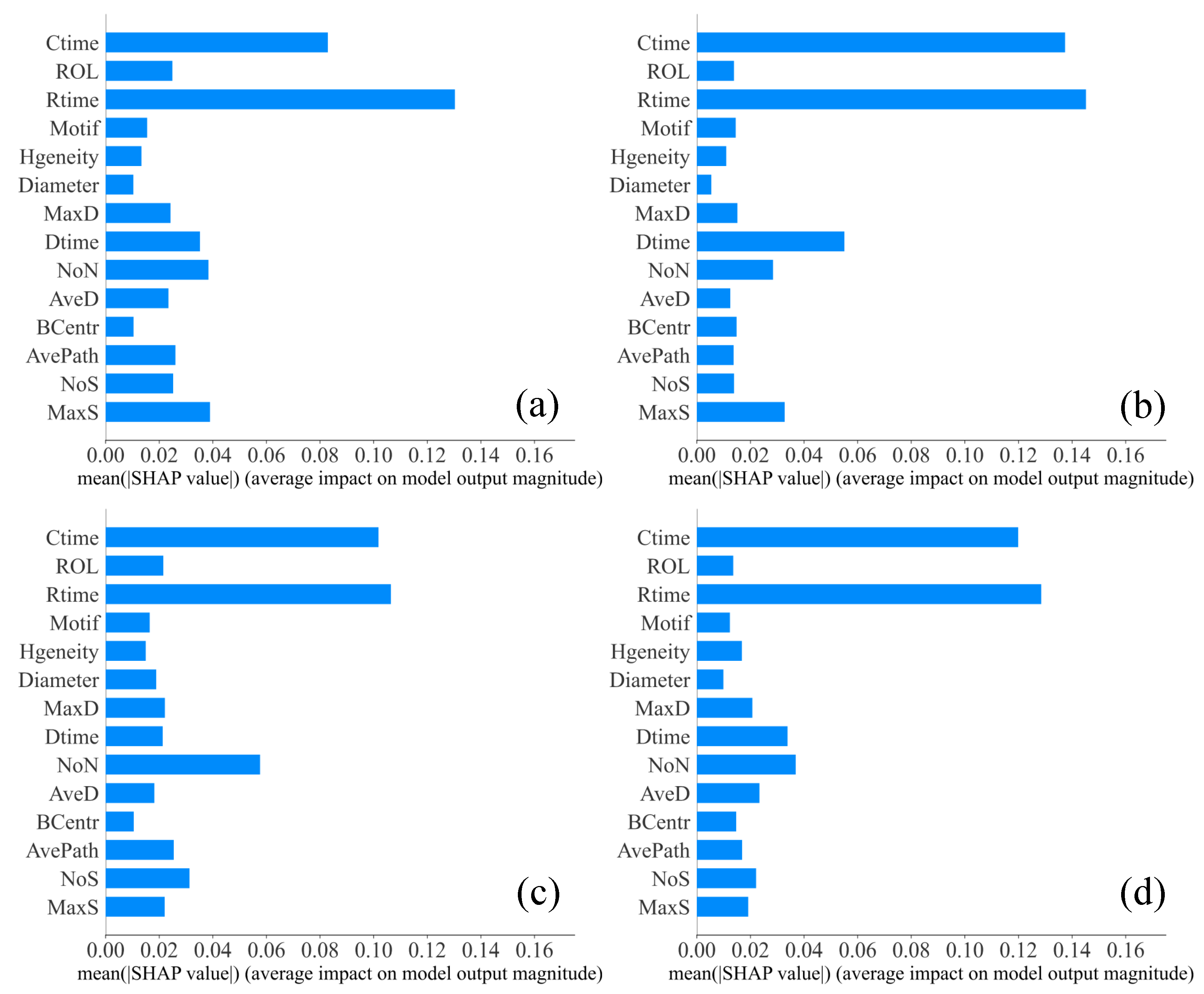
To intuitively show the change in features in the sampled datasets and the original datasets, we calculate the mean (|SHAP value|) based on Random Forest on the sampled and the original datasets, where denotes the absolute value, and the larger the mean (|SHAP value|) is, the more critical the corresponding features are. Figure 5 and Figure 6 demonstrate the mean (|SHAP value|) changes with the subsampling of skewness. Comparing the Characteristic time and Network diameter (Diameter), the mean (|SHAP value|) on the subsampled Gossipcop dataset (Figure 5a,b) is larger than that on the original Gossipcop dataset (Figure 5c,d). This result shows that the importance of features does change after the matching method. Meanwhile, comparing most of the features (i.e., Characteristic time (Ctime), Average shortest path (AvePath), and Tweet number in largest subgraph (MaxS)), the mean (|SHAP value|) does not change in the subsampled Gossipcop dataset (Figure 5a,b) while these features are different for the original Gossipcop dataset (Figure 5c,d), which indicates that the feature drift disappears in the subsampled Gossipcop dataset. Furthermore, as shown in Figure 6, the importance of the features does not change significantly between the subsampled and original datasets for the Twitter dataset, which implies that the difference in distribution may be the reason for the feature drift phenomenon.
Overall, by controlling the distribution of tweets’ creation times, we find that the phenomenon of feature drift disappears on Gossipcop, and the feature importance becomes closer between the two subsampled datasets, which implies that the difference in the distribution of the tweets’ creation time plays an important role in the feature drift phenomenon.
Although SHAP and PDP could be used to interpret fake news detection methods and prove the existence of the feature drift phenomenon, they are global interpretable models that are costly when the data size is large. Fortunately, Anchors [55] provides a local interpretable perspective. Anchors is a local model-agnostic interpretability algorithm based on ‘if-then’ rules, which has high precision and clear coverage of the black-box model. The method of Anchors can be easily understood as follows: given an instance x to be explained, a rule (or an anchor) A that applies to x is to be found, while the prediction of x’s neighbors is the same as x‘s under a high probability (which means ‘precision’ in Anchors). The definition of ‘coverage’ in Anchors represents the correct probability of x’s neighbors.
Table 4 shows the application of Anchors for the Gossipcop and Twitter datasets before and after sampling. Taking the original data of Gossipcop in 2.4 h as an example, it can be intuitively interpreted that if the feature values satisfy ‘Average shortest path (AvePath) > 1.94 AND Number of nodes ≤ 56.00’, the precision of true news is 0.92, and the results cover of the nearby instances. This anchor shows that in 2.4 h, Average shortest path is effective in detecting fake news and the decision boundary is 1.94, which is similar to the results in Figure 3. In the case of the cut-off time equal to 12 h, the most effective feature of the original Gossipcop dataset is Network diameter (Diameter). Thus, the different decision features also verify the feature drift on the original Gossipcop dataset. In contrast to the Twitter dataset before sampling, the decision feature given by Anchors is Characteristic time (Ctime) for both cut-off times, and the decision boundary does not change notably over time, which indicates that feature drift is not visible on the Twitter dataset.
The anchor of the Gossipcop dataset changed significantly after sampling, i.e., in the case of the cut-off times of 2.4 h and 12 h, Characteristic time (Ctime) and Average shortest path (AvePath) become the most effective features, and the decision boundaries are closer for both features under the two cut-off times. This result corresponds to the phenomenon that the mean (|SHAP value|) of the two features is the largest among all features in Figure 5a,b, and the result also indicates that the feature drift phenomenon disappears in the sampling Gossipcop dataset.
In summary, the Anchors method offers a local perspective to interpret the importance of the features easily and exhibit the decision boundaries in models. By utilizing the Anchors method to supplement the interpretation of feature drift, we intuitively observe that the feature drift phenomenon disappears in the sampling datasets, which is consistent with the results when using mean (|SHAP value|) on the two sampling datasets.
5. Conclusions
Fake news on social networks threatens the credibility of information and triggers social panic, leading to serious negative consequences. Therefore, fake news detection technology plays an important role in today’s society. However, the traditional fake news detection models pay more attention to the accuracy of the models on specific datasets and ignore the interpretability of the models. The low interpretability of the model may hinder fact-checkers’ judgments and it cannot be applied to other fake news datasets. In this work, we first make an assumption that the phenomenon of feature drift may widely appear in fake news detection algorithms, which leads to a poor transfer effect. Then, we adopt interpretability methods (i.e., SHAP and PDP) to verify the feature drift phenomenon. Finally, our work proposes an innovative skewness-matching sampling method and creates two sampled datasets with the same skewness distribution. The results show that the feature drift phenomenon disappears in the sampled datasets, which verifies the notion that the distribution of the tweets’ creation time may be one reason for feature drift. Generally speaking, our study provides an interpretable analysis for feature drift in fake news detection and reveals the potential relationship between feature drift and datasets, which could help researchers when transferring fake news detection algorithms. In addition, although, in this work, we designed a data-independent interpretable method to interpret feature drift, we did not design an effective fake news detection algorithm to avoid feature drift, and this will be the direction of our future work.
Author Contributions
C.F. and X.P. wrote the main manuscript text. C.F., X.X., S.Y. and Y.M. conceived the experiments. C.F., X.P. and X.L. conducted the experiments. All authors analyzed the results and reviewed the manuscript. All authors have read and agreed to the published version of the manuscript.
Funding
This work was supported by the Zhejiang Provincial Natural Science Foundation of China (Grants LGF21G010003 and LGF20F020016) and the National Natural Science Foundation of China (Grants 62173065 and 62103374).
Institutional Review Board Statement
Not applicable.
Informed Consent Statement
Not applicable.
Data Availability Statement
Not applicable.
Conflicts of Interest
The authors declare no conflict of interest.
References
- Zhou, X.; Zafarani, R. Fake news: A survey of research, detection methods, and opportunities. arXiv 2018, arXiv:1812.00315v1. [Google Scholar]
- Fu, C.; Xia, Y.; Yue, X.; Yu, S.; Min, Y.; Zhang, Q.; Leng, Y. A Novel Spatiotemporal Behavior-Enabled Random Walk Strategy on Online Social Platforms. IEEE Trans. Comput. Soc. Syst. 2021, 9, 807–817. [Google Scholar] [CrossRef]
- Fu, C.; Yue, X.; Shen, B.; Yu, S.; Min, Y. Patterns of interest change in stack overflow. Sci. Rep. 2022, 12, 1–10. [Google Scholar] [CrossRef]
- Alam, S.; Ravshanbekov, A. Sieving fake news from genuine: A synopsis. arXiv 2019, arXiv:1911.08516. [Google Scholar]
- Lazer, D.M.; Baum, M.A.; Benkler, Y.; Berinsky, A.J.; Greenhill, K.M.; Menczer, F.; Metzger, M.J.; Nyhan, B.; Pennycook, G.; Rothschild, D.; et al. The science of fake news. Science 2018, 359, 1094–1096. [Google Scholar] [CrossRef]
- Bovet, A.; Makse, H.A. Influence of fake news in Twitter during the 2016 US presidential election. Nat. Commun. 2019, 10, 1–14. [Google Scholar] [CrossRef] [PubMed] [Green Version]
- Silverman, C. This Analysis Shows How Wiral Fake Election News Stories Outperformed Real News on Facebook; BuzzFeed News: New York, NY, USA, 2016. [Google Scholar]
- Pogue, D. How to Stamp Out Fake News. Sci. Am. 2017, 316, 24. [Google Scholar] [CrossRef]
- Allcott, H.; Gentzkow, M. Social media and fake news in the 2016 election. J. Econ. Perspect. 2017, 31, 211–236. [Google Scholar] [CrossRef] [Green Version]
- Liu, Y.; Jin, X.; Shen, H.; Cheng, X. Do rumors diffuse differently from non-rumors? A systematically empirical analysis in sina weibo for rumor identification. In Proceedings of the Pacific-Asia Conference on Knowledge Discovery and Data Mining, Jeju, Republic of Korea, 23–26 May 2017; Springer: Berlin/Heidelberg, Germany, 2017; pp. 407–420. [Google Scholar]
- Vosoughi, S.; Roy, D.; Aral, S. The spread of true and false news online. science 2018, 359, 1146–1151. [Google Scholar] [CrossRef]
- Meyers, M.; Weiss, G.; Spanakis, G. Fake News Detection on Twitter Using Propagation Structures. In Proceedings of the Multidisciplinary International Symposium on Disinformation in Open Online Media, Online, 26–27 October 2020; Springer: Berlin/Heidelberg, Germany, 2020; pp. 138–158. [Google Scholar]
- Rubin, V.L. On deception and deception detection: Content analysis of computer-mediated stated beliefs. Proc. Am. Soc. Inf. Sci. Technol. 2010, 47, 1–10. [Google Scholar] [CrossRef]
- Törnberg, P. Echo chambers and viral misinformation: Modeling fake news as complex contagion. PLoS ONE 2018, 13, e0203958. [Google Scholar] [CrossRef] [PubMed]
- Zhou, X.; Zafarani, R. A survey of fake news: Fundamental theories, detection methods, and opportunities. ACM Comput. Surv. (CSUR) 2020, 53, 1–40. [Google Scholar] [CrossRef]
- Guess, A.; Nagler, J.; Tucker, J. Less than you think: Prevalence and predictors of fake news dissemination on Facebook. Sci. Adv. 2019, 5, eaau4586. [Google Scholar] [CrossRef] [PubMed] [Green Version]
- Tsfati, Y.; Boomgaarden, H.G.; Strömbäck, J.; Vliegenthart, R.; Damstra, A.; Lindgren, E. Causes and consequences of mainstream media dissemination of fake news: Literature review and synthesis. Ann. Int. Commun. Assoc. 2020, 44, 157–173. [Google Scholar] [CrossRef]
- Kucharski, A. Study epidemiology of fake news. Nature 2016, 540, 525. [Google Scholar] [CrossRef] [Green Version]
- Volkova, S.; Shaffer, K.; Jang, J.Y.; Hodas, N. Separating facts from fiction: Linguistic models to classify suspicious and trusted news posts on twitter. In Proceedings of the 55th Annual Meeting of the Association for Computational Linguistics (Volume 2: Short Papers), Vancouver, BC, Canada, 30 July–4 August 2017; Association for Computational Linguistics: Stroudsburg, PA, USA, 2017; pp. 647–653. [Google Scholar]
- Bond, G.D.; Holman, R.D.; Eggert, J.A.L.; Speller, L.F.; Garcia, O.N.; Mejia, S.C.; Mcinnes, K.W.; Ceniceros, E.C.; Rustige, R. ‘Lyin’Ted’, ‘Crooked Hillary’, and ‘Deceptive Donald’: Language of Lies in the 2016 US Presidential Debates. Appl. Cogn. Psychol. 2017, 31, 668–677. [Google Scholar] [CrossRef]
- Gogate, M.; Adeel, A.; Hussain, A. Deep learning driven multimodal fusion for automated deception detection. In Proceedings of the 2017 IEEE Symposium Series on Computational Intelligence (SSCI), Honolulu, HI, USA, 27 November–1 December 2017; IEEE: Piscataway, NJ, USA, 2017; pp. 1–6. [Google Scholar]
- Li, L.; Qin, B.; Ren, W.; Liu, T. Document representation and feature combination for deceptive spam review detection. Neurocomputing 2017, 254, 33–41. [Google Scholar] [CrossRef]
- Ren, Y.; Ji, D. Neural networks for deceptive opinion spam detection: An empirical study. Inf. Sci. 2017, 385, 213–224. [Google Scholar] [CrossRef]
- Ma, J.; Gao, W.; Wong, K.F. Rumor detection on twitter with tree-structured recursive neural networks. In Proceedings of the 56th Annual Meeting of the Association for Computational Linguistics. Association for Computational Linguistics, Melbourne, Australia, 15–20 July 2018; pp. 1980–1989. [Google Scholar]
- Kwon, S.; Cha, M.; Jung, K. Rumor detection over varying time windows. PLoS ONE 2017, 12, e0168344. [Google Scholar] [CrossRef] [Green Version]
- Choudhary, A.; Arora, A. Linguistic feature based learning model for fake news detection and classification. Expert Syst. Appl. 2021, 169, 114171. [Google Scholar] [CrossRef]
- Wang, W.Y. ‘Liar, Liar Pants on Fire’: A New Benchmark Dataset for Fake News Detection. In Proceedings of the 55th Annual Meeting of the Association for Computational Linguistics (Volume 2: Short Papers), Vancouver, BC, Canada, 30 July–4 August 2017; Association for Computational Linguistics: Stroudsburg, PA, USA, 2017; pp. 422–426. [Google Scholar]
- Tu, K.; Chen, C.; Hou, C.; Yuan, J.; Li, J.; Yuan, X. Rumor2vec: A rumor detection framework with joint text and propagation structure representation learning. Inf. Sci. 2021, 560, 137–151. [Google Scholar] [CrossRef]
- Liang, B.; Li, H.; Su, M.; Bian, P.; Li, X.; Shi, W. Deep Text Classification Can Be Fooled. In Proceedings of the 27th International Joint Conference on Artificial Intelligence IJCAI’18, Stockholm, Sweden, 13–19 July 2018; AAAI Press: Washington, DC, USA, 2018; pp. 4208–4215. [Google Scholar]
- Zhou, X.; Zafarani, R. Network-based fake news detection: A pattern-driven approach. ACM SIGKDD Explor. Newsl. 2019, 21, 48–60. [Google Scholar] [CrossRef]
- Silva, A.; Han, Y.; Luo, L.; Karunasekera, S.; Leckie, C. Propagation2Vec: Embedding partial propagation networks for explainable fake news early detection. Inf. Process. Manag. 2021, 58, 102618. [Google Scholar] [CrossRef]
- Davoudi, M.; Moosavi, M.R.; Sadreddini, M.H. DSS: A hybrid deep model for fake news detection using propagation tree and stance network. Expert Syst. Appl. 2022, 198, 116635. [Google Scholar] [CrossRef]
- Liu, Y.; Wu, Y.F.B. Early detection of fake news on social media through propagation path classification with recurrent and convolutional networks. In Proceedings of the Thirty-Second AAAI Conference on Artificial Intelligence, New Orleans, LA, USA, 2–7 February 2018. [Google Scholar]
- Shu, K.; Cui, L.; Wang, S.; Lee, D.; Liu, H. defend: Explainable fake news detection. In Proceedings of the 25th ACM SIGKDD International Conference on Knowledge Discovery & Data Mining, Anchorage, AK, USA, 4–8 August 2019; pp. 395–405. [Google Scholar]
- Lundberg, S.M.; Lee, S.I. A unified approach to interpreting model predictions. Adv. Neural Inf. Process. Syst. 2017, 30, 4765–4774. [Google Scholar]
- Hastie, T.; Tibshirani, R.; Friedman, J.H.; Friedman, J.H. The Elements of Statistical Learning: Data Mining, Inference, and Prediction; Springer: Berlin/Heidelberg, Germany, 2009; Volume 2. [Google Scholar]
- Doshi-Velez, F.; Kim, B. Towards a rigorous science of interpretable machine learning. arXiv 2017, arXiv:1702.08608. [Google Scholar]
- Molnar, C. Interpretable Machine Learning. A Guide for Making Black Box Models Explainable; Independently published; 2022; ISBN 979-8411463330. [Google Scholar]
- Du, M.; Liu, N.; Hu, X. Techniques for interpretable machine learning. Commun. ACM 2019, 63, 68–77. [Google Scholar] [CrossRef] [Green Version]
- Kingsford, C.; Salzberg, S.L. What are decision trees? Nat. Biotechnol. 2008, 26, 1011–1013. [Google Scholar] [CrossRef]
- Weisberg, S. Applied Linear Regression; John Wiley & Sons: Hoboken, NJ, USA, 2005; Volume 528. [Google Scholar]
- Ribeiro, M.T.; Singh, S.; Guestrin, C. “Why should i trust you?” Explaining the predictions of any classifier. In Proceedings of the 22nd ACM SIGKDD International Conference on Knowledge Discovery and Data Mining, San Francisco, CA, USA, 13–17 August 2016; Association for Computing Machinery: New York, NY, USA, 2016; pp. 1135–1144. [Google Scholar]
- Singhal, S.; Kabra, A.; Sharma, M.; Shah, R.R.; Chakraborty, T.; Kumaraguru, P. Spotfake+: A multimodal framework for fake news detection via transfer learning (student abstract). In Proceedings of the AAAI Conference on Artificial Intelligence, New York, NY, USA, 7–12 February 2020; Volume 34, pp. 13915–13916. [Google Scholar]
- Fu, C.; Zheng, Y.; Liu, Y.; Xuan, Q.; Chen, G. NES-TL: Network embedding similarity-based transfer learning. IEEE Trans. Netw. Sci. Eng. 2019, 7, 1607–1618. [Google Scholar] [CrossRef]
- Lu, Y.J.; Li, C.T. GCAN: Graph-aware Co-Attention Networks for Explainable Fake News Detection on Social Media. In Proceedings of the 58th Annual Meeting of the Association for Computational Linguistics, Online, 5–10 July 2020; Association for Computational Linguistics: Stroudsburg, PA, USA, 2020; pp. 505–514. [Google Scholar] [CrossRef]
- Ma, J.; Gao, W.; Wong, K.F. Detect rumors in microblog posts using propagation structure via kernel learning. In Proceedings of the 5th Annual Meeting of the Association for Computational Linguistics. Association for Computational Linguistics, Vancouver, BC, Canada, 30 July–4 August 2017; Association for Computational Linguistics: Stroudsburg, PA, USA, 2017; pp. 708–717. [Google Scholar]
- Shu, K.; Mahudeswaran, D.; Wang, S.; Liu, H. Hierarchical propagation networks for fake news detection: Investigation and exploitation. In Proceedings of the International AAAI Conference on Web and Social Media, Atlanta, GA, USA, 8–11 June 2020; Volume 14, pp. 626–637. [Google Scholar]
- Wu, K.; Yang, S.; Zhu, K.Q. False rumors detection on sina weibo by propagation structures. In Proceedings of the 2015 IEEE 31st International Conference on Data Engineering, Seoul, Republic of Korea, 13–17 April 2015; IEEE: Piscataway, NJ, USA, 2015; pp. 651–662. [Google Scholar]
- Barabási, A.L. Network Science; Cambridge University Press: Cambridge, UK, 2016. [Google Scholar]
- Zhao, Z.; Zhao, J.; Sano, Y.; Levy, O.; Takayasu, H.; Takayasu, M.; Li, D.; Wu, J.; Havlin, S. Fake news propagates differently from real news even at early stages of spreading. EPJ Data Sci. 2020, 9, 7. [Google Scholar] [CrossRef]
- Albert, R.; Barabási, A.L. Statistical mechanics of complex networks. Rev. Mod. Phys. 2002, 74, 47. [Google Scholar] [CrossRef] [Green Version]
- Dong, J.; Horvath, S. Understanding network concepts in modules. BMC Syst. Biol. 2007, 1, 24. [Google Scholar] [CrossRef] [PubMed] [Green Version]
- Zhang, J.; Tang, J.; Zhong, Y.; Mo, Y.; Li, J.; Song, G.; Hall, W.; Sun, J. Structinf: Mining structural influence from social streams. In Proceedings of the AAAI Conference on Artificial Intelligence, San Francisco, CA, USA, 4–9 February 2017; Volume 31. [Google Scholar]
- Fu, C.; Zhao, M.; Fan, L.; Chen, X.; Chen, J.; Wu, Z.; Xia, Y.; Xuan, Q. Link weight prediction using supervised learning methods and its application to yelp layered network. IEEE Trans. Knowl. Data Eng. 2018, 30, 1507–1518. [Google Scholar] [CrossRef]
- Ribeiro, M.T.; Singh, S.; Guestrin, C. Anchors: High-precision model-agnostic explanations. In Proceedings of the AAAI Conference on Artificial Intelligence, New Orleans, LA, USA, 2–7 February 2018; Volume 32. [Google Scholar]
Figure 1.
The performance of four baseline algorithms on the Twitter (a) and the Gossipcop (b) datasets.
Figure 1.
The performance of four baseline algorithms on the Twitter (a) and the Gossipcop (b) datasets.

Figure 2.
SHAP summary plots for the Twitter and Gossipcop datasets. (a,b) refer to the Twitter dataset, (c,d) refer to the Gossipcop dataset. The cut-off times are (a,c) 2.4 h and (b,d) 12 h.
Figure 2.
SHAP summary plots for the Twitter and Gossipcop datasets. (a,b) refer to the Twitter dataset, (c,d) refer to the Gossipcop dataset. The cut-off times are (a,c) 2.4 h and (b,d) 12 h.

Figure 3.
Partial dependency plot for the Gossipcop dataset. (a) Cut-off time is 2.4 h. (b) Cut-off time is 12 h. The shaded area represents the confidence interval.
Figure 3.
Partial dependency plot for the Gossipcop dataset. (a) Cut-off time is 2.4 h. (b) Cut-off time is 12 h. The shaded area represents the confidence interval.

Figure 4.
The distribution of creation time in two datasets.

Figure 5.
Mean (|SHAP value|) on the subsampled and original Gossipcop datasets at different cut-off times. (a,b) On the subsampled Gossipcop dataset, the cut-off time is 2.4 h and 12 h, respectively. (c,d) On the original Gossipcop dataset, the cut-off time is 2.4 h and 12 h, respectively.
Figure 5.
Mean (|SHAP value|) on the subsampled and original Gossipcop datasets at different cut-off times. (a,b) On the subsampled Gossipcop dataset, the cut-off time is 2.4 h and 12 h, respectively. (c,d) On the original Gossipcop dataset, the cut-off time is 2.4 h and 12 h, respectively.

Figure 6.
Mean (|SHAP value|) of the subsampled and original Twitter datasets for different cut-off times. (a,b) On the subsampled Twitter dataset, the cut-off time is 2.4 h and 12 h, respectively. (c,d) On the original Twitter dataset, the cut-off time is 2.4 h and 12 h, respectively.
Figure 6.
Mean (|SHAP value|) of the subsampled and original Twitter datasets for different cut-off times. (a,b) On the subsampled Twitter dataset, the cut-off time is 2.4 h and 12 h, respectively. (c,d) On the original Twitter dataset, the cut-off time is 2.4 h and 12 h, respectively.


Table 1.
Statistics of the datasets.
| Gossipcop | ||
|---|---|---|
| True news | 205 | 6945 |
| Fake news | 205 | 3684 |
| Users | 173,487 | 739,166 |
| Tweets | 204,820 | 1,058,330 |
Table 2.
Temporal features.
| Temporal Features | Description |
|---|---|
| Ctime | Characteristic time. It captures how fast the retweet behavior is among the propagation graph. The specific definition is shown in Section 3.2. |
| Dtime | Max-degree time. The creation time of the node whose degree value is maximum in the graph, which indicates the time when the propagation reaches a key node. |
| Rtime [48] | Response time, which captures the timeliness of the response. The expression is as in Equation (1). |
Table 3.
Structural features.
| Structural Features | Description |
|---|---|
| MaxD [49] | Maximum degree value in the propagation graph. |
| ROL [50] | Ratio of layer sizes. The number of nodes whose distance is 2 to the publisher divided by the number whose distance is 1. |
| BCentr [49] | Average value of betweenness centrality of all nodes. |
| Diameter [51] | Network diameter. The maximum distance between nodes in the propagation graph. |
| AveD [51] | Average degree. The average value of degrees of all nodes in the propagation graph. |
| AvePath [51] | Average shortest path. The average value of the distance of all node pairs in the propagation graph. |
| NoN [49] | Number of nodes in the propagation graph. |
| NoS [49] | Number of subgraphs in the propagation graph. |
| MaxS [49] | Tweet number in the largest subgraph. The number of tweets in the largest subgraph. |
| Hgeneity [52] | Structural heterogeneity, which indicates the connectivity of the propagation graph. The expression is as in Equation (3). |
| Motif [53] | Depth motif degree, which analyzes the graph structure from the micro perspective. The expression is as in Equation (4). |
Table 4.
Anchors interpretations.
| Dataset | Anchors | Precision | Coverage |
|---|---|---|---|
| Gossipcop (2.4 h) | Average shortest path > 1.94 AND Number of nodes ≤ 56.00 | 0.92 | 0.03 |
| Gossipcop (12 h) | Diameter ≤ 3.00 | 0.88 | 0.42 |
| Gossipcop (2.4 h subsampled) | Characteristic time ≤ 147.77 AND Average shortest path ≤ 2.00 | 0.95 | 0.30 |
| Gossipcop (12 h subsampled) | Characteristic time ≤ 148.52 AND Average shortest path ≤ 2.03 | 0.97 | 0.40 |
| Twitter (2.4 h) | Characteristic time ≤ 91.63 AND Ratio of layer > 0.76 | 1.00 | 0.11 |
| Twitter (12 h) | Characteristic time ≤ 98.09 AND Diameter ≤ 9.00 | 0.97 | 0.09 |
| Twitter (2.4 h subsampled) | Characteristic time ≤ 50.9 AND Response time > 0.01 | 0.86 | 0.08 |
| Twitter (12 h subsampled) | Characteristic time ≤ 84.40 AND Response time > 0.05 | 0.94 | 0.40 |
Disclaimer/Publisher’s Note: The statements, opinions and data contained in all publications are solely those of the individual author(s) and contributor(s) and not of MDPI and/or the editor(s). MDPI and/or the editor(s) disclaim responsibility for any injury to people or property resulting from any ideas, methods, instructions or products referred to in the content. |
© 2023 by the authors. Licensee MDPI, Basel, Switzerland. This article is an open access article distributed under the terms and conditions of the Creative Commons Attribution (CC BY) license (https://creativecommons.org/licenses/by/4.0/).
Share and Cite
MDPI and ACS Style
Fu, C.; Pan, X.; Liang, X.; Yu, S.; Xu, X.; Min, Y. Feature Drift in Fake News Detection: An Interpretable Analysis. Appl. Sci. 2023, 13, 592. https://0-doi-org.brum.beds.ac.uk/10.3390/app13010592
AMA Style
Fu C, Pan X, Liang X, Yu S, Xu X, Min Y. Feature Drift in Fake News Detection: An Interpretable Analysis. Applied Sciences. 2023; 13(1):592. https://0-doi-org.brum.beds.ac.uk/10.3390/app13010592
Chicago/Turabian StyleFu, Chenbo, Xingyu Pan, Xuejiao Liang, Shanqing Yu, Xiaoke Xu, and Yong Min. 2023. "Feature Drift in Fake News Detection: An Interpretable Analysis" Applied Sciences 13, no. 1: 592. https://0-doi-org.brum.beds.ac.uk/10.3390/app13010592
Note that from the first issue of 2016, this journal uses article numbers instead of page numbers. See further details here.