
Three-Dimensional Processing of Reflections for Passive-Source Seismology Based on Geometric Design


School of Geophysics and Information Technology, China University of Geosciences (Beijing), Beijing 100083, China
*
Author to whom correspondence should be addressed.
Appl. Sci. 2023, 13(10), 6126; https://0-doi-org.brum.beds.ac.uk/10.3390/app13106126
Submission received: 18 March 2023
/
Revised: 15 May 2023
/
Accepted: 15 May 2023
/
Published: 17 May 2023
(This article belongs to the Special Issue Technological Advances in Seismic Data Processing and Imaging)
Abstract
:Passive-source exploration is a method of seismic exploration that has loose requirements on the conditions of the surface, is cheap, and does not require excitation by an active source. The ambient seismic signals collected from the field over an extended period of time can be used to generate virtual-shot seismic records similar to those obtained from the seismic exploration of an active source based on the relevant correlations, and this can in turn yield information on the underground structure through a series of conventional methods of processing seismic data. Three-dimensional (3D) processing can mitigate the influence of the azimuth of random noise to yield a more representative underground structure, but requires intensive computation. In this paper, we propose a 3D method to compute reflections of a passive source based on the geometry of seismic exploration. Assuming a high quality of imaging, we use information on the predesigned geometry to choose and correlate noisy synthetic data on the reflections by a seismic body to create virtual shot data, and subsequently capture images of the 3D data on passive reflection. The use of the predesigned geometry ensures that only the important and useful parts of the dataset are used for correlation and imaging, where this reduces the cost of computation. The proposed method can thus efficiently generate high-quality 3D synthetic data.
1. Introduction
Passive-source seismic exploration, which is based on seismic wave interferometry, was developed by Schuster [1] and Bakulin and Calvert [2]. This method is different from active-source seismic exploration in that it does not require excitation by an artificial source or knowledge of the number and locations of the sources. Correlations can be used to convert environmental seismic noise or micro-earthquakes into a determined seismic response. The theory of seismic interferometry involves “perform[ing] correlations on the seismic records received by receivers at two points on the surface, and the results can be regarded as the records of the wave field of the active source, with one point as the receiver and the other point as the source” [3,4]. Applying this calculation to all random signals of the receiver can yield a group of virtual shot records of the passive source that are similar to forward records of the active source in seismic exploration.
Methods of passive-source seismic exploration can be divided into techniques for investigating passive-source surface waves [5,6,7] and passive-source body waves [3,8,9,10,11], according to the types of seismic waves. Because the Earth absorbs body waves to a much greater extent than surface waves, it is much more difficult to capture images of the former than the latter [12]. Some researchers have retrieved reflections of waves from ambient noise by using illumination-based diagnosis [13,14], while others have sought to improve the quality of data on reflections of the passive source [15,16,17,18,19].
Methods of exploring reflections of the passive source have been applied in many areas. Masatoshi et al. [20] calculated the velocities of the P-wave and the S-wave, the bundle factor of the P-wave, and other structural parameters based on seismic noise in field data obtained from observation wells in Cold Lake, Alberta, Canada. Seismic wave interference technology was used to investigate the presence of metal ores by Cheraghi et al. [21]. Cheraghi et al. [22] applied passive source exploration to the four-dimensional dynamic monitoring of carbon dioxide storage sites at an Aquistore facility. Eric et al. [23] used data on underground activity in a mine and vibrations of the ventilation pipes in the context of exploring mining resources, and Brenguier et al. [24] used the noise in waves generated by a railway to monitor the shallow crust. Brenguier et al. [25] also used a receiver array to monitor long-term seismic velocity and anticipate geological events.
According to the theory of passive seismic exploration, sources of random noise are needed to evenly identify geological targets from all directions and obtain accurate kinematical results. Artifacts may be obtained when the source is not located along the direction of the receiver line [14]. Three-dimensional (3D) passive-source seismic exploration can be used to obtain more uniform information and images of better quality than two-dimensional (2D) passive seismic exploration. Draganov et al. [12] and Nakata et al. [26] obtained the underground velocity from environmental noise by using seismic wave interference technology and generated a corresponding 3D seismic profile. Chamarczuk et al. [27] used the full-scale 3D seismic method of the virtual source survey to explore the Kylylahti polymetallic mine in Finland and obtained geological information that could not be obtained through active seismic exploration.
While 3D passive seismic reflections have delivered promising results, they require intensive computations as well as a large storage space for the data obtained. Given these issues, we propose a method to calculate images of 3D reflections based on the geometric design of the area. We use information on the area, the surface, and the underground structure to design a reasonable geometry for it, subsequently use that to screen for effective data to obtain correlations, and finally generate an imaging profile with uniform folds and azimuths. The passive-source direct migration method is another means to improve computational efficiency. It was proposed by Artman [28] and has been applied to passive seismic exploration [29,30,31,32]. The passive-source direct migration method does not generate correlations to obtain virtual shot records, but directly performs migration imaging to obtain records of random noise and improve computational efficiency.
2. Extracting 3D Virtual Shot Records Based on Geometry
2.1. Principle of Reflection of Waves from Passive Sources
Interferometry is the basis of calculations for passive seismic exploration and can be derived from the equation of the acoustic wave according to the reciprocity theorem [31,32]:
where is Green’s function of the observation points and in the frequency domain, is the angular frequency, is a random source, and and are the velocity and the density of medium, respectively. and are random signals received by the receivers, represents the superposition of the results of the mutual interferometry of different windows, and is calculated by taking the real part.
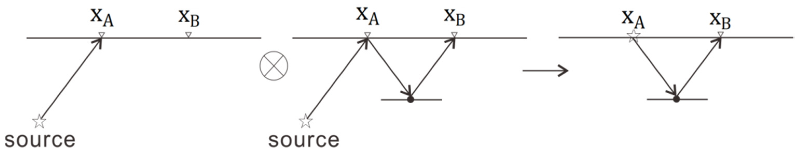
Figure 1 shows that the above formula can be used to obtain virtual shot records similar to those due to excitation by an active source, with one point as the source and the other as the receiver, by performing interferometry on two points of the passive source. If point A does not move, and point B is transformed, we can obtain virtual shot records with point A as the source.
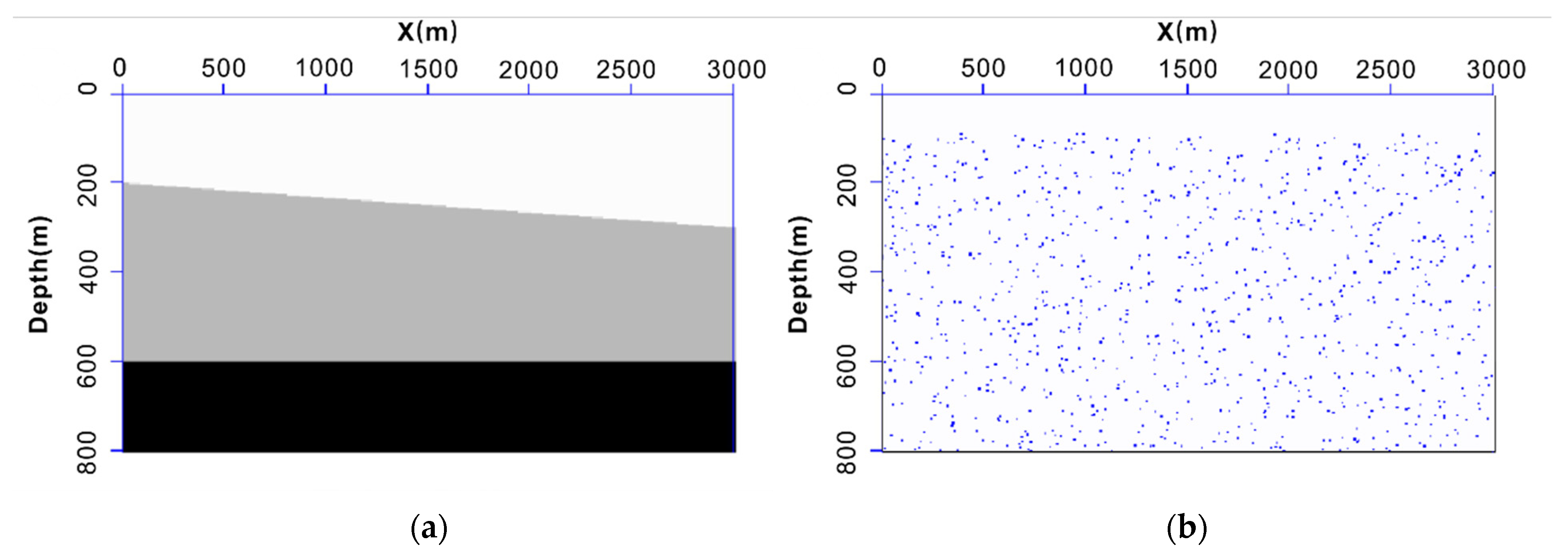
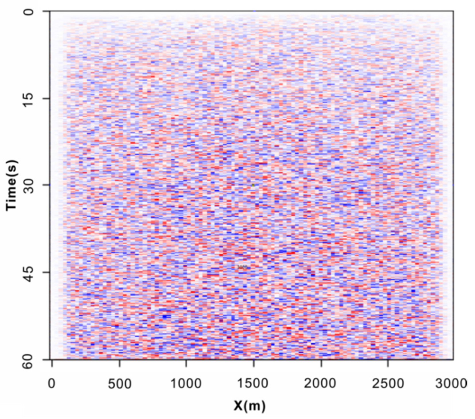
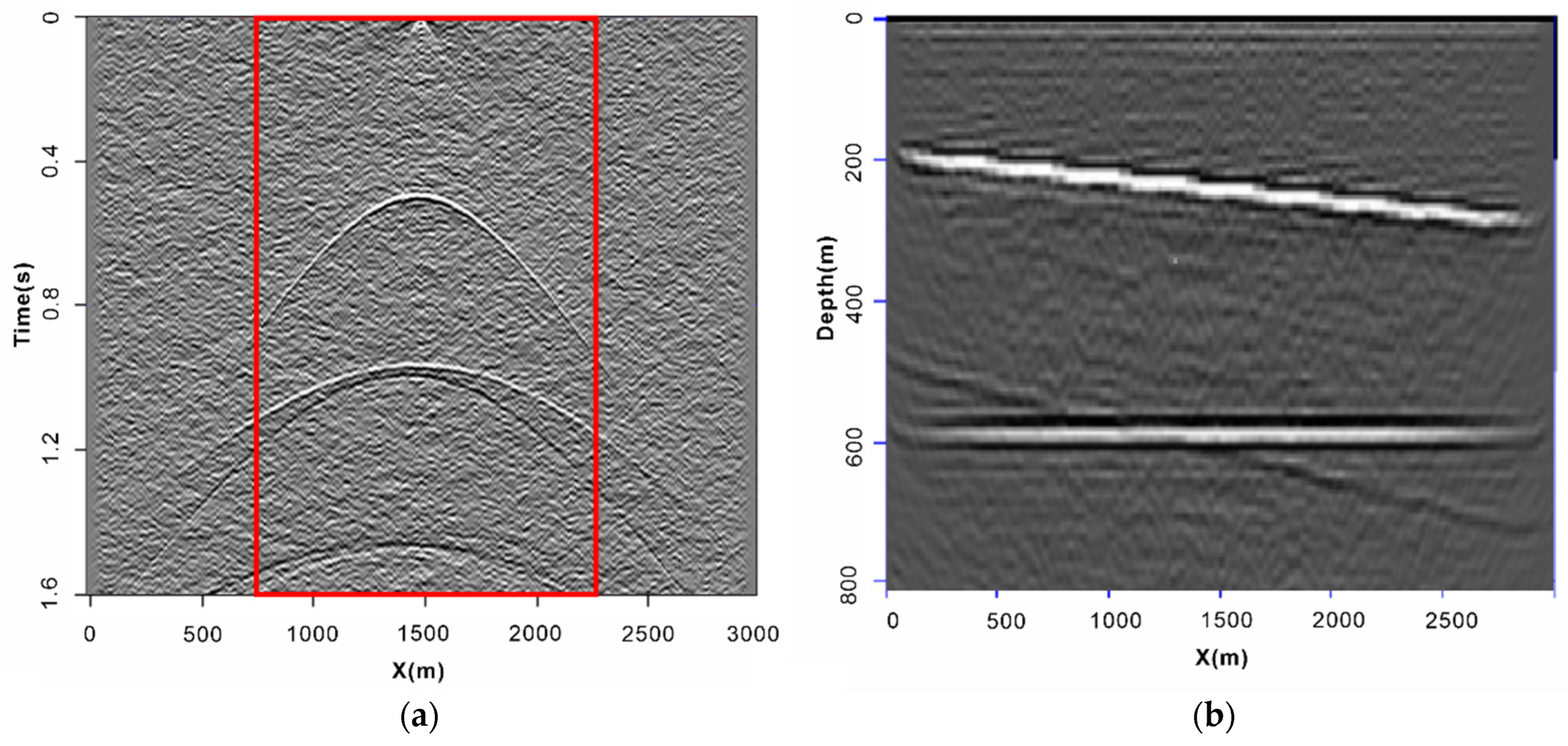
We use a 2D forward model of a passive source to illustrate the process of extraction of the virtual shot records of the reflections by the passive source. We established a model of velocity as shown in Figure 2a, with a length of 3000 m, a depth of 800 m, and a grid spacing of dx = dz = 10 m. The lower, left, and right boundaries of the model were the boundaries of absorption, and we set 31 absorption layers. The upper boundary was a free boundary. The model contained three geological horizons with velocities of 1000, 2500, and 4000 m/s from top to bottom. A receiver was arranged after every 10 m on the surface, with a total of 301 receivers. There were 2000 sources of random noise (Figure 2b), and 60 s of random noise records were obtained through forward modeling (Figure 3). The source was made to continuously shake during acquisition, and its amplitudes and phases were completely random. Each of the channels of random noise was related to the other 300 channels. That is, one channel of the seismic record of a virtual source was chosen as the source, and the others were used as receivers (Figure 4a). The signal-to-noise ratios (SNRs) of the near-offset data in the red box in the figure were high. The profile of migration was obtained, as shown in Figure 4b, by calculating all 301 respective channels, using the conventional method of processing seismic data.
2.2. Calculating 3D Virtual Shot Records of Passive Source Based on Geometry
The core of passive seismic reflection exploration is to obtain virtual shot records based on correlations between a channel of ambient noise records and other channels. When the length of the correlation is given, the ambient seismic records received over a long time need to be divided into several windows according to this length, and can then be correlated and stacked. To reconstruct a high-fidelity Green function, the time series of mutual correlation among the seismic data is usually very long. This makes it necessary to increase the number of folds to improve the quality of the Green function, which in turn reduces the computational efficiency of imaging of the passive source. Therefore, the number of virtual shot records, length of the ambient seismic records, length of the correlation window, and number of seismic channels involved in the calculation all influence the time needed to generate the virtual shot records.
Passive seismic exploration using reflections of waves from the source is based on correlations between all channels of random signals, and the generated virtual shot records are similar to those of an active source. They should also comply with the corresponding requirements of geometric design in theory. An appropriate geometry can not only improve the quality of imaging, but can also reduce the computational expense. Many seismic channels are involved in correlation and stacking in the calculation of virtual shot records, and the long time needed to record the ambient noise incurs a high computational intensity. The range of seismic channels needed to obtain correlations in 2D calculations is usually selected by setting the spacing and range of offset of points on the source. However, a rule is required in case of 3D calculations to ensure the quality of the generated virtual shot records. The data processing features uniform folds, wide azimuths, and other requirements that are similar to those for active seismic exploration. The geometric design has been extensively studied in the context of conventional seismic exploration, and exploration based on reflections from a passive source can directly learn from the experience accumulated by this research. We designed a method to compute the virtual shot records of reflections from a 3D passive source based on the design of the geometry for active-source seismic data to ensure a sufficient number of folds and quality of imaging while reducing the computational cost.
Before acquiring 3D data on the active source for seismic exploration, the geometry required to determine how to position the sources and receivers can be designed according to the known surface and the underground geological conditions of the given area. One can then specify the location of each source and receiver and the corresponding relationships between them. Following this, we must ensure that the collected data contain uniform folds, and then set the range of the offset distance and the azimuths. The geometric design usually considers the geological target elements and cost of acquisition. The file containing these geometric data is usually called the Shell Processing Support (SPS) Format for 3D Land Survey, and is a standard file for recording information on the source and the receiver as well as their relationship. The SPS file is mainly composed of a source-information file (S file, Table 1), a receiver-information file (R file, Table 2), and a source–receiver relationship file (X file, Table 3). The SPS file determines the unique physical location of the sources and receivers in the working area as well as their relationships. In the context of correlations, the SPS.S file stores information on the sources of all virtual shot records, and the SPS.X file contains the range of the receivers in the SPS.R file that need to be correlated with these sources.
The difference between the geometry of the reflections from a passive source and that used in conventional seismic exploration should be considered to formulate the geometric design. Because each point representing a receiver in passive seismic exploration can become a point representing a source through correlation, the density of the points representing the source in passive seismic exploration may be much higher than that in active seismic exploration. On the premise of satisfying the requirements related to the number of folds and the SNR of the data, it is thus necessary to set an appropriate number of passive sources and receivers to significantly reduce the cost of processing.
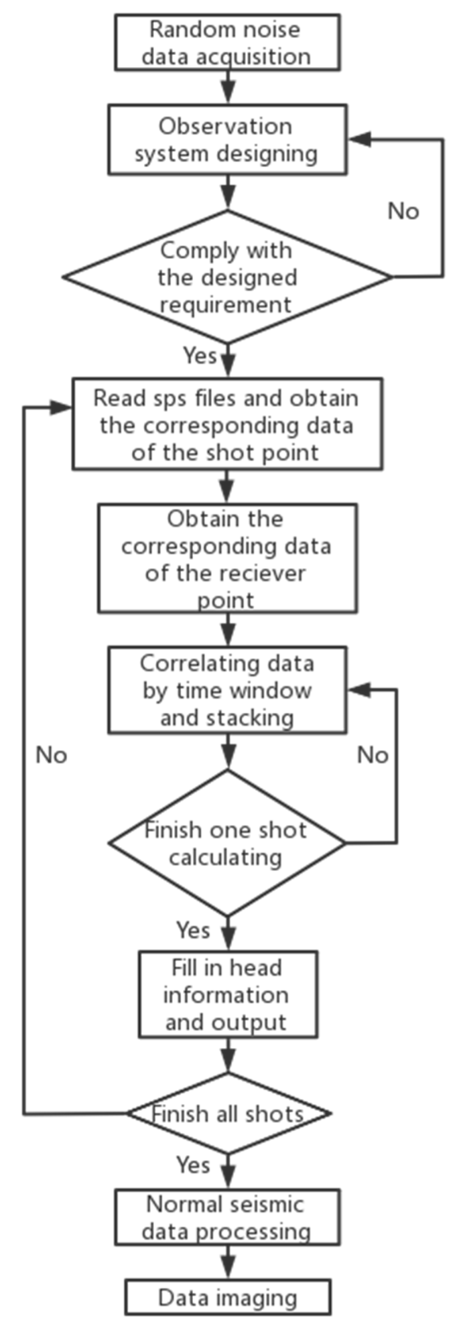
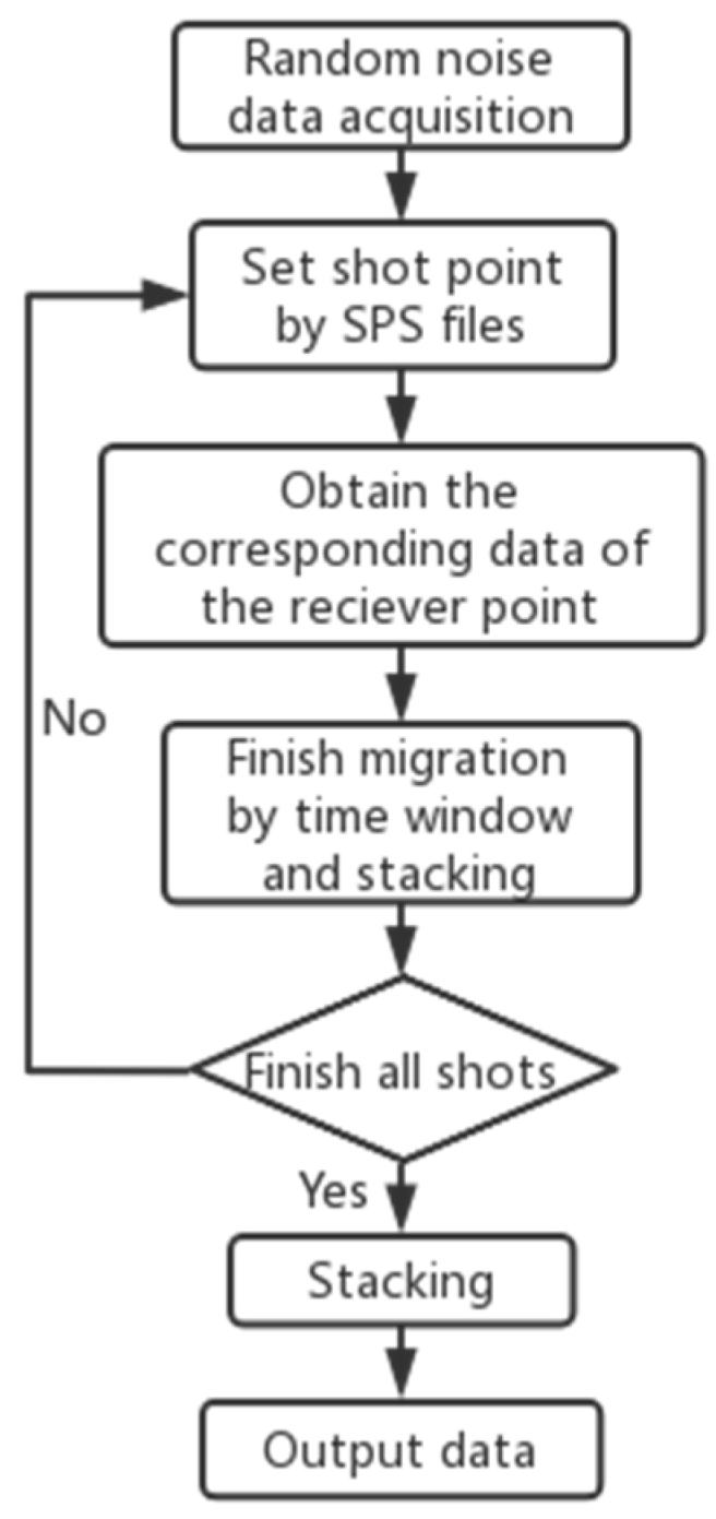
Based on the above requirements, we propose a method to generate virtual shot records of 3D reflections from a passive source based on the above-mentioned geometry file, as shown in Figure 5. The procedure is as follows: (1) Having collected random noise records from the field, a geometry with a sufficient number of folds and uniform azimuths should be designed by using a design software according to the known surface, information on the underground structure, and geological targets, and should be stored in the SPS file. (2) The information is obtained on the source and receivers from the SPS.X file. The length of the correlation should be determined according to the conditions of the working area. After completion of the generation of virtual data for a receiver from its related shots, the initial data of this receiver are obtained for one correlation time. Then, we slide the time window by a correlation time, and repeat the above process until the end of the random noise records. By vertically stacking all of the correlation results, we can obtain the seismic record of this receiver. Following this, the remaining receivers corresponding to the source are calculated to obtain one shot of the virtual seismic records. (3) The entire SPS.X file is read to obtain all of the virtual shot records according to the previous step, and the imaging section is then obtained by processing seismic records of reflections of waves from the passive source according to the conventional method of processing.
2.3. Model Test
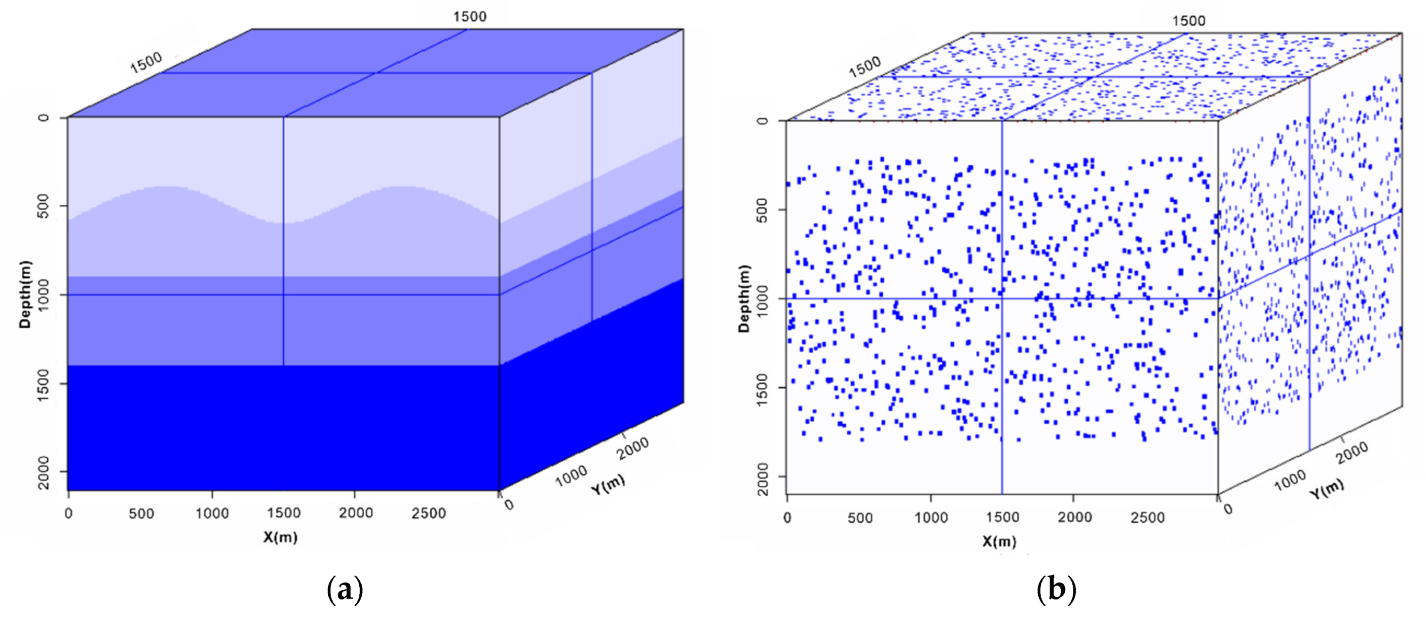
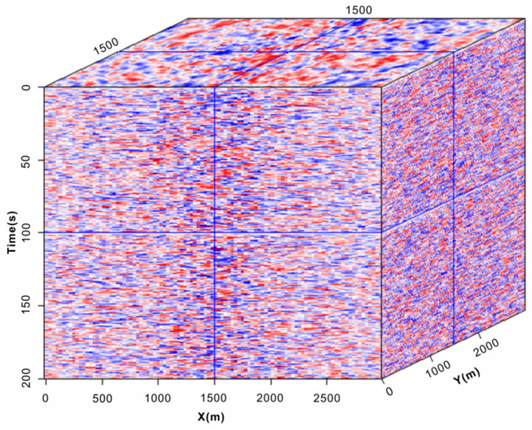
We designed a forward model to verify the theory of 3D passive seismic exploration. The size of the model was 3000 m × 3000 m × 2100 m, and the grid spacing dx = dy = dz = 30 m. The model consisted of four geological horizons with velocities of 1000, 1600, 2500, and 4000 m/s from top to bottom, as shown in Figure 6a. As we sought to study reflections from the source in deep layers, we used the acoustic finite-difference algorithm to generate data on ambient noise, and randomly set 160,000 sources in the range of 200–1800 m from the model, as shown in Figure 6b. A survey line was arranged every 30 m on the surface, and 100 receivers were arranged for each survey line. A total of 10,000 receivers were thus set, that is, the distance between the receivers in both the x and the y directions was 30 m. The seismic waves were stimulated at randomly distributed sources, and a total of 200 s of seismic records were collected by the receivers on the surface (shown in Figure 7). During acquisition, the source was made to continuously shake at random amplitudes and phases. This was done to simulate the collection of noise records of reflections from a passive source by the surface receivers.
2.3.1. Conventional Forward Model
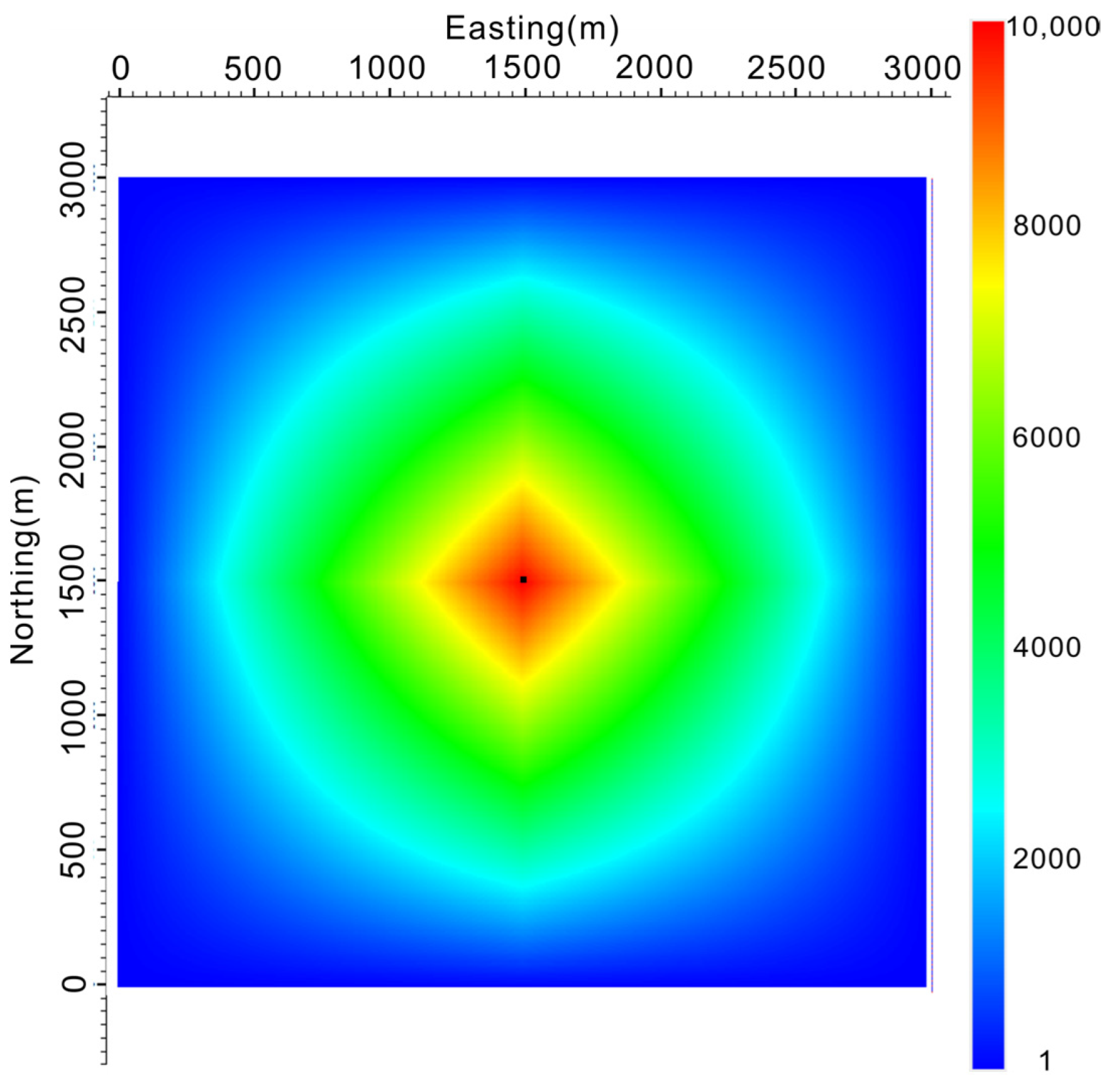
All data from each receiver are successively used according to the time window as the source to obtain the correlations and stack them with data from the other receivers to generate a group of virtual shot records in the conventional method. The proposed geometry is shown in Figure 8. It is clear from the map of the folds that the maximum number of folds of the virtual shot records was 10,000, and gradually decreased from the center of the working area to the surrounding area. The 5050th source and receiver lines 50–52 of the seismic records were extracted. We can clearly see the non-phase axial morphology of the reflections and its conformance to the model as well as the low SNR of the far-offset part. Figure 9 shows the results of processing one shot of the virtual shot records. It yielded the imaging section that was stacked by using conventional seismic processing, with 40 s as the time window of correlation.
2.3.2. Forward Model with a Narrow Azimuth
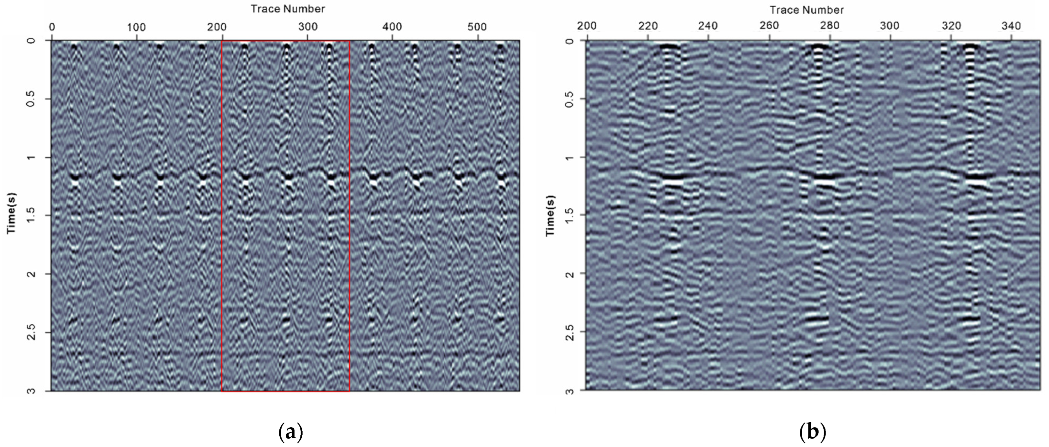
According to the proposed scheme and the method for active seismic exploration, we designed a geometry with a narrow azimuth: The maximum offset along the inline direction was 1500 m, and that along the crossline direction was 300 m, that is, each shot was recorded by 51 × 11 receivers at most, and the aspect ratio was 0.2. Figure 10a shows the source point and the range of its corresponding receiver point, and Figure 10b shows the folds of the geometry designed on the basis of this scenario. Figure 11a shows the records collected by using this geometry at the center of the model, Figure 11b shows the part of the shot records in the red box in Figure 11a, and Figure 12 shows the results of migration imaging and stacking, performed by calculating shot records by extracting one line of every four, with 40 s as the time window of correlation. The velocities required for migration and nmo were obtained from the model of velocity.
2.3.3. Forward Model with a Wide Azimuth
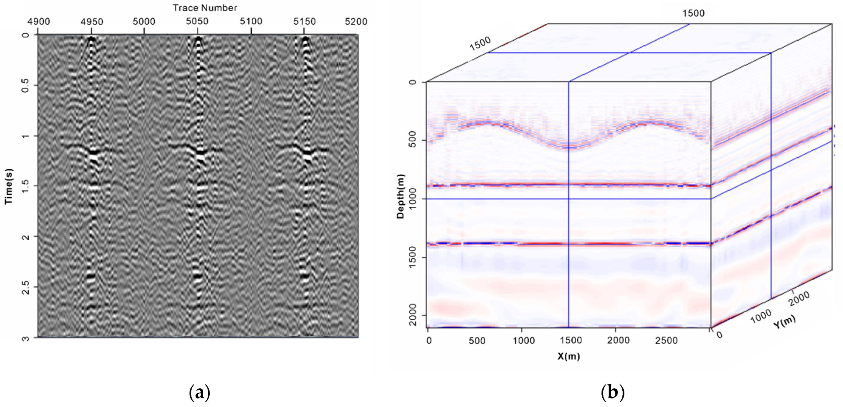
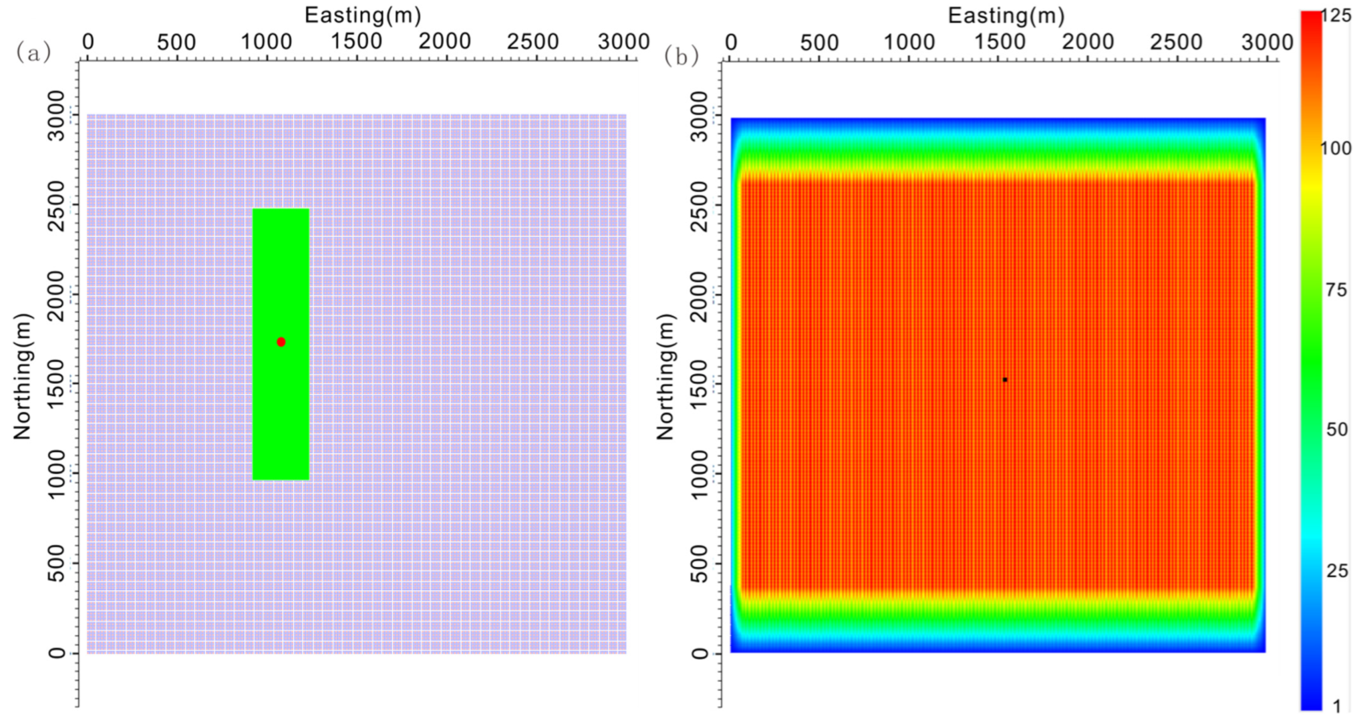
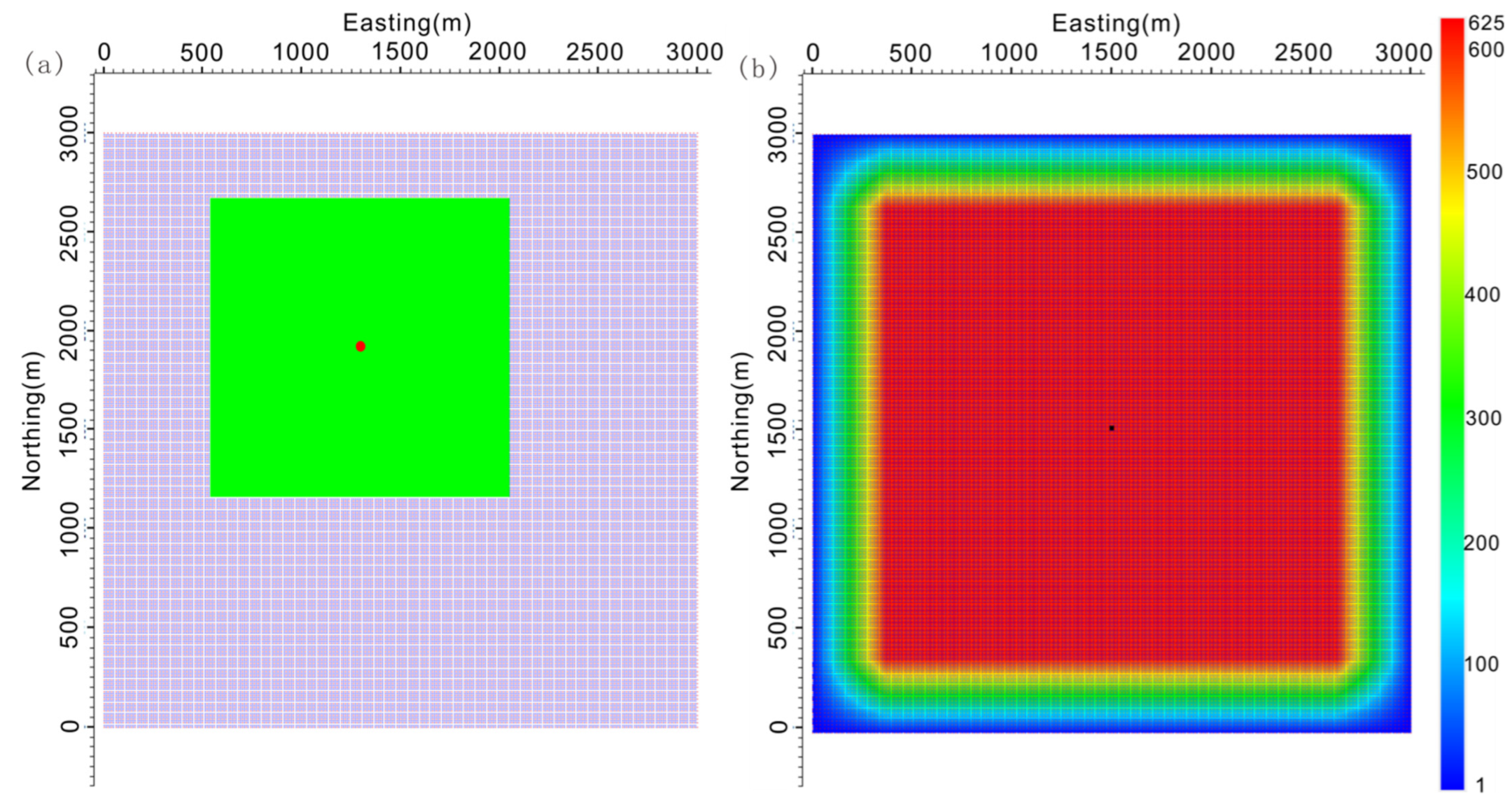
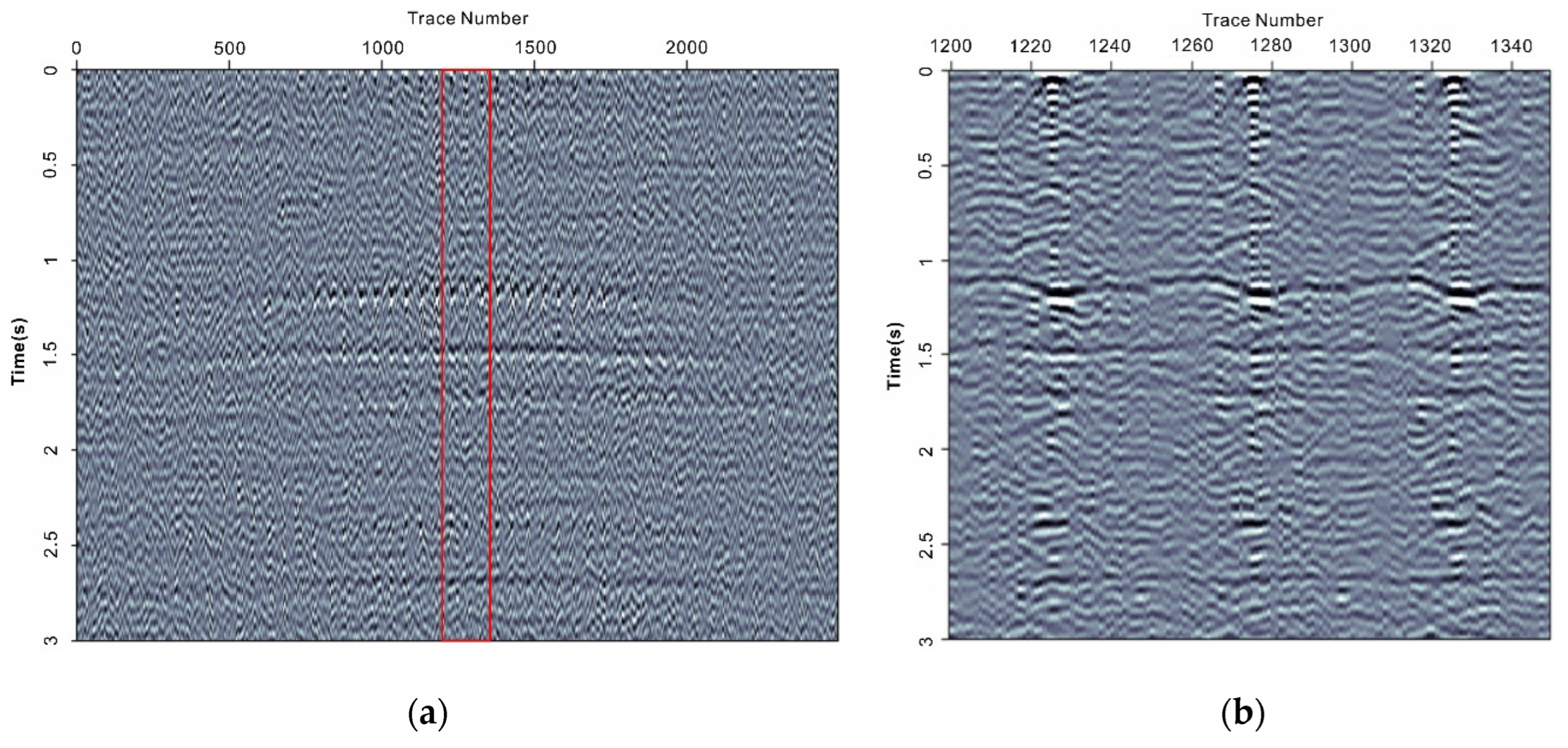
We also designed a geometry with a wide azimuth: The maximum offsets along the direction of the line and the direction vertical to it were both 1500 m, that is, each source received data from 51 × 51 receivers at most, and the aspect ratio was one. Figure 13a shows the source point and the range of its corresponding receiver point, and Figure 13b shows folds of the geometry designed on the basis of this scenario. Figure 14a shows the shot records collected by using this geometry at the center of the model, and Figure 14b shows shot records depicted by the red box in Figure 14a. Figure 15 shows the results of migration imaging and stacking, performed by calculating shot records by extracting one line from every four with a time window of correlation of 40 s. The velocities required for the migration and nmo were obtained from the model of velocity.
A comparison of the complete model (Figure 9b), narrow azimuth model (Figure 12) and wide azimuth model (Figure 15) shows that the three methods generated similar migration profiles by using a model-compliant geometry and the processing workflow of conventional seismic exploration, and their results were consistent with the 3D model of velocity in Figure 6a. This shows that the proposed method of generating virtual shot records of a 3D passive source based on SPS files is accurate. Due to the geometric design, data based on narrow and wide azimuths from all receiver points are not needed to participate in the calculation of each source, which significantly reduces the computation time (narrow azimuth model and wide azimuth model took about 1/20 and 1/4, respectively, of the time taken to calculate the virtual shot records by using all of the receiver points) and ensures uniform folds.
3. Direct Migration of Reflections of 3D Waves from Passive Source Based on Geometry
3.1. Principle of Calculation of Direct Migration
The principle of calculating random noise by direct migration can be expressed as follows:
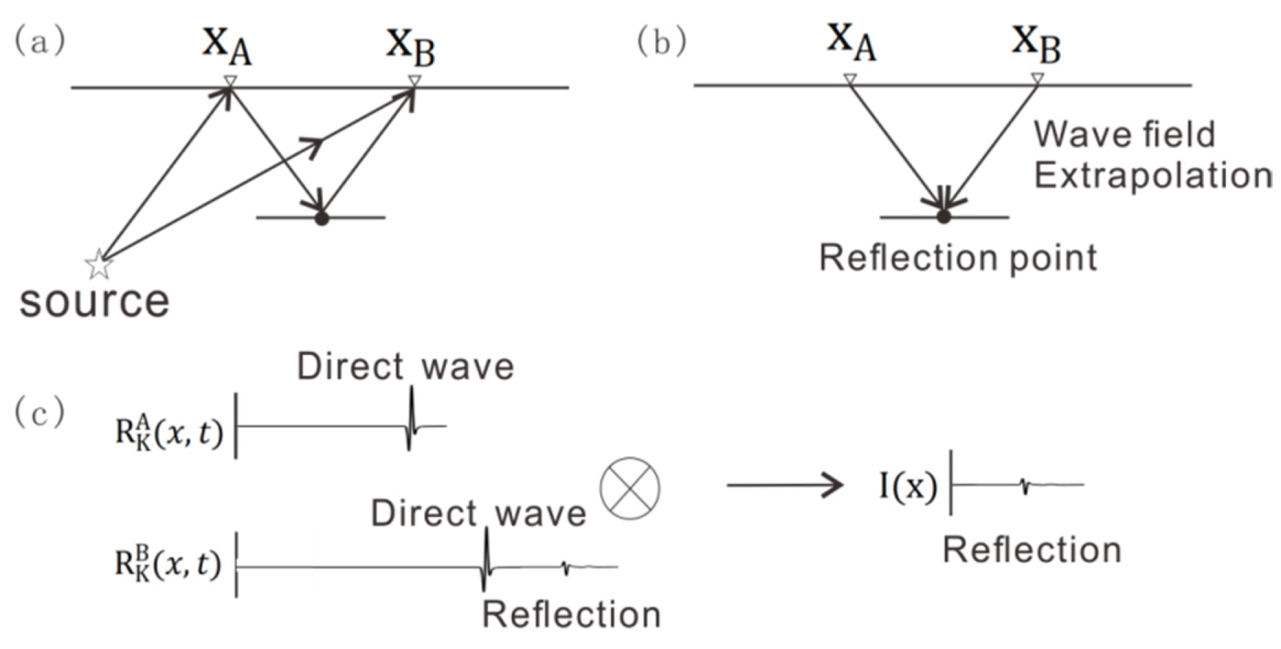
and are the wave fields from the kth (k = 1, 2, …, ) source at a certain time, and are received by the receivers and on the surface. The two are extended downward, and the underground image of the reflection can be obtained through correlation (Figure 16). The final result of imaging is the sum of the results of correlation of a series of sources and receivers in a series of time windows. Artman [27] summarized the process of calculation of direct migration of data from a passive source as the extrapolation, correlation, and summation of the wave field. All algorithms for migration imaging that involve the extrapolation of the wave field and are conducive for use in the relevant imaging conditions can apply the direct migration method
We used the one-way wave pre-stack depth migration method to process the original random noise records. It consisted of two steps: recursion of the source and receiver points along the direction of the depth, and imaging [33] to satisfy the requirements of the direct migration method.
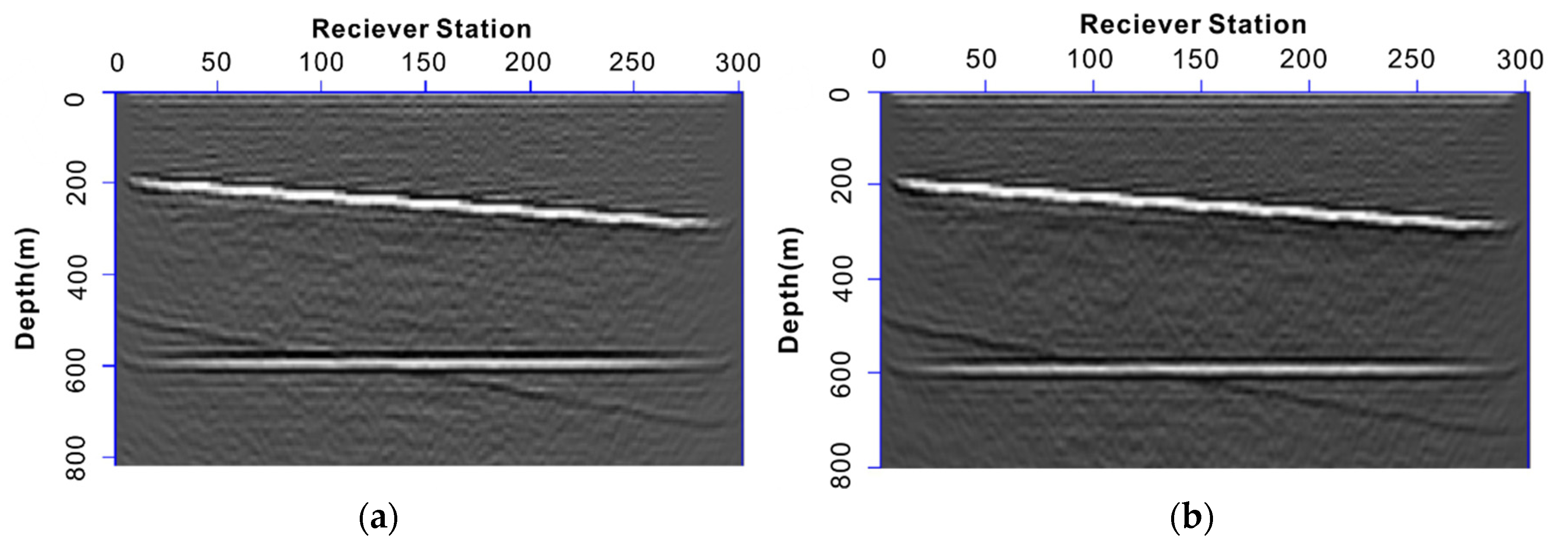
The forward calculation of the 2D passive source by using direct migration was carried out by using the models of velocity and random noise records described in Section 2, and shown in Figure 2 and Figure 3, to illustrate the process of imaging of the reflections by the passive source. One of the random noise records was set as the source point, with the remaining records used for one-way wave migration. All 301 data sources were calculated and stacked, and the migration profile was obtained by using conventional seismic processing, as shown in Figure 17.
One channel of the random noise records was set as the source point, and the other 300 channels were set as receiver points, that is, the range of geometry included all of the data. Performing one-way wave migration and stacking for all 301 “sources” and models of velocity yielded a direct migration profile (Figure 17b). The results were consistent with those of migration imaging based on the conventional processing of the 2D passive source in Figure 17a. That is, the direct migration imaging of reflections by a passive source was accurate, and the proposed method is thus feasible.
3.2. Calculation of 3D Reflections from a Passive Source Using Direct Migration Based on Geometry
The process of calculating the 3D reflection from a passive source by using direct migration based on the geometry is similar to the method of generating virtual shot records of reflections from a 3D passive source based on the relevant geometry file, as shown in Figure 18:
- Having collected random noise records from the field, the geometry that satisfies the given requirements is designed by using a design software according to the known surface and information on the underground structure as well as the geological targets, and is stored in the SPS file.
- A random noise record is set at a specified location as the noise record of the source point according to the content of the SPS.S file. The range of the corresponding receiver point is obtained from the SPS.X file according to the source point. The noise records of all receiver points are read, the one-way wave offset is calculated, stacking according to the time window is performed, and the information stored in the SPS.S file and SPS.R files is inserted into the header.
- All of the results of the migration of virtual shot records are calculated, and the imaging section is obtained after processing the stack.
3.3. Testing the Model of Direct Migration
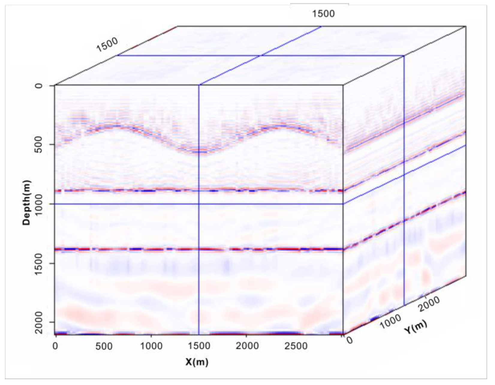
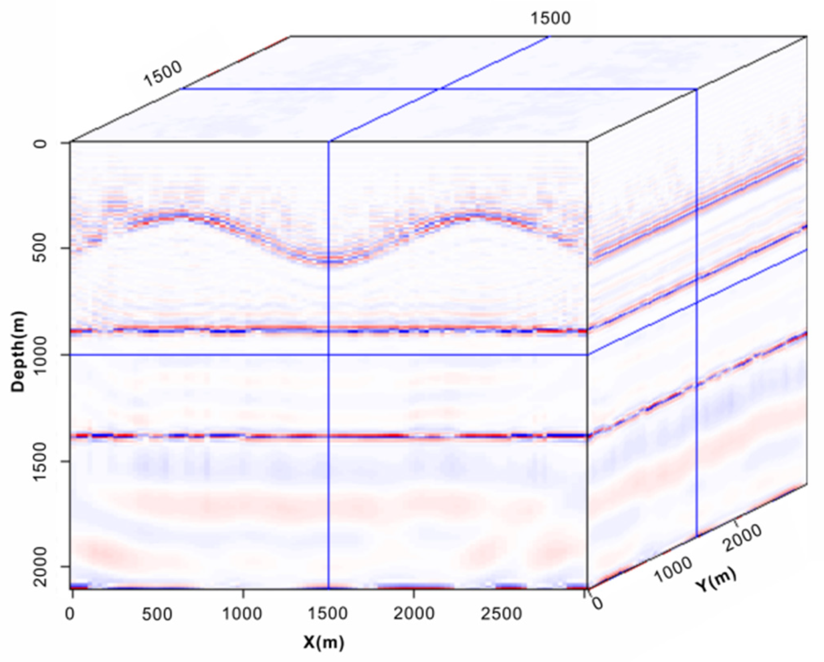
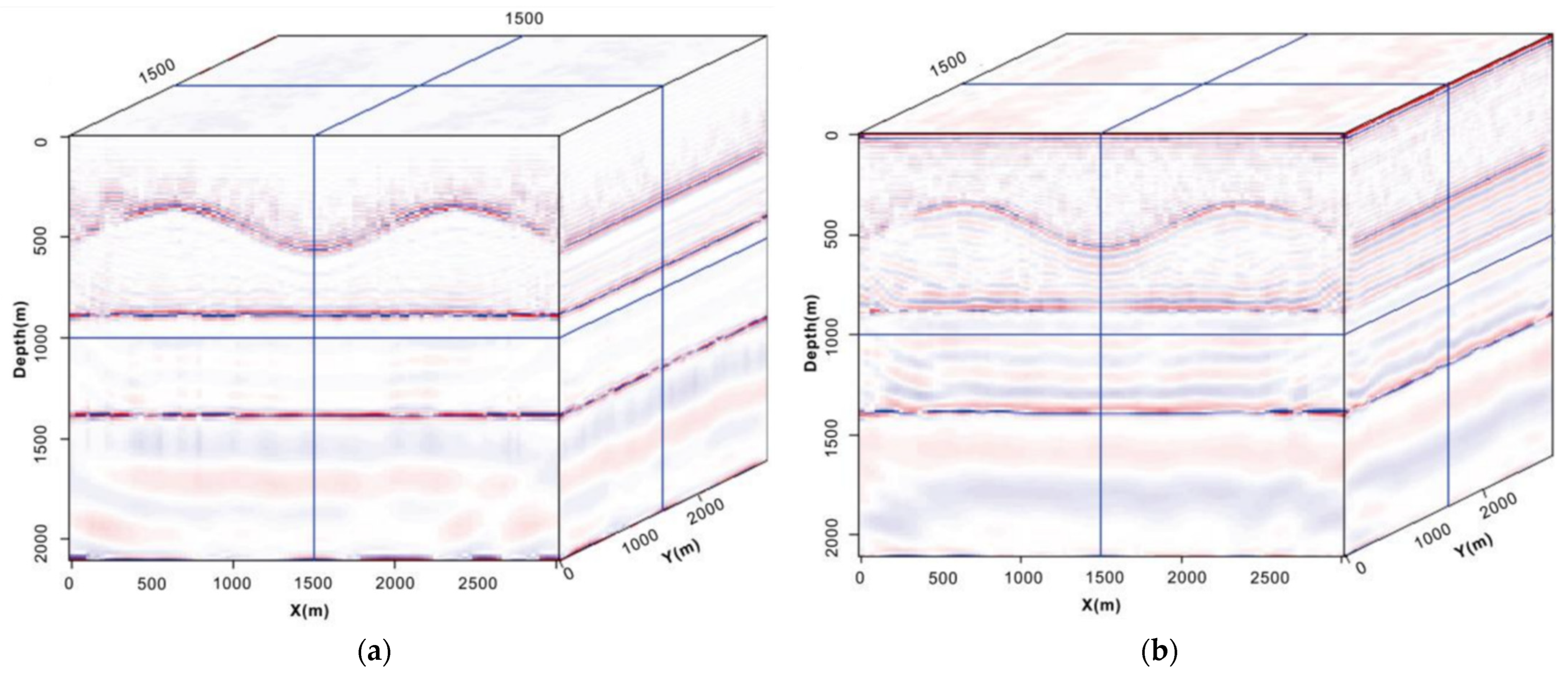
The model of velocity (Figure 6a) and the random noise records (Figure 7) described in the previous section were used to conduct an experiment on the direct migration of random reflection-induced noise. The process of calculation is shown in Figure 18. A geometry with a wide azimuth was used, as shown in Figure 14. The maximum offset along the inline direction and the crossline direction was 1500 m, that is, the signal from each source was received by 51 × 51 receivers at most, and the aspect ratio was one. One line was extracted from every four for the calculations. After reading the SPS.X file, the source points of the data on the offset noise were placed in the channels described in the file, and the corresponding seismic channels of the receiver point in the SPS.X file were extracted to calculate the one-way wave migration with a time window of 20 s. The final migration profile obtained by stacking all of the results of migration is shown in Figure 19b. The velocities required for the migration and nmo were taken from the model of velocity. The results obtained by the conventional method of passive seismic exploration were consistent with those based on calculating the direct migration of reflections. The direct migration method required less computational and storage-related resources, and was accurate.
When the forward migration-based imaging is carried out by using a geometry with a wide azimuth, there is no need for all sources or receivers to participate in the calculation; this significantly reduces the time needed for computations and yields uniform folds. By applying this geometry, we used only 1/4 of the source lines, and each source used only 1/4 of the near-offset receivers (the computational time was only about 1/16 of that incurred when using the entire dataset). As shown in Figure 18, the 3D seismic records obtained by the wide-azimuth geometry were processed by the direct migration method and yielded results of imaging similar to those of the virtual shot records of reflections from a passive source by using the migration method. This indicates that the proposed method can obtain accurate migration profiles by omitting the correlation in the virtual shot records, and thus requires less time and computational resources.
4. Conclusions
Seismic exploration based on reflections from a passive source uses the imaging of background noise, is cheap, and can be used as an effective supplement to methods of exploring deep active seismic sources. However, its computational cost and storage-related requirements constitute constraints on its further development.
Using a geometry based on the given geological structure can solve the above problem in practice. A set of geometric parameters that are suitable for the given area can reduce the cost of acquisition and the difficulty of data processing while improving their resolution. In this paper, we used experience in processing data on seismic exploration based on reflections from a 3D active source to design a reasonable and efficient geometry to obtain data for a 3D passive source. On the premise of ensuring a high signal-to-noise ratio, uniform folds, and reasonable azimuth, we used SPS files to guide the relevant correlations and obtain the virtual shot records; this improved the computational efficiency. At the same time, we obtained data on reflections of waves from the 3D passive source through forward modeling, and generated a clear seismic profile by calculating according to the above process.
In addition, we tested the feasibility of imaging based on direct migration using random reflection-induced noise. The method of generating virtual shot records is similar to the migration imaging algorithm based on correlation-based imaging conditions, that is, this method of migration can omit the correlations in the virtual shot records, thus reducing the requisite computational resources and storage space and improving efficiency. After intercepting multiple, random time windows of noise for multiple folds, the results also yielded images of high quality. The proposed method is thus efficient in terms of the seismic exploration of a passive source based on reflections.
The proposed method can accelerate the calculation of reflections from a passive source, and its many virtues can help promote the use of such technology on a large scale.
Author Contributions
Conceptualization, Y.L.; Software, Y.L.; Validation, Y.L.; Writing–original draft, Y.L.; Project administration, G.L.; Funding acquisition, G.L. All authors have read and agreed to the published version of the manuscript.
Funding
This study was supported by the NSFC (Grant No. 42074131), and the National Key R&D Program of China (Grant Nos. 2021YFC2801404 and 2022YFC280016803).
Institutional Review Board Statement
Not applicable.
Informed Consent Statement
Not applicable.
Data Availability Statement
Not applicable.
Conflicts of Interest
The authors declare no conflict of interest.
References
- Schuster, G.T. Theory of daylight/ interferometric imaging: Tutorial. In Proceedings of the 63rd EAGE Conference & Exhibition, Amsterdam, The Netherlands, 11–15 June 2001; p. A32, Extended Abstracts. [Google Scholar]
- Bakulin, A.; Calvert, R. Virtual source: New method for imaging and 4D below complex overburden. In Proceedings of the 74th Annual International Meeting, SEG, Denver, Colorado, 10–15 October 2004; pp. 2477–2480, Expanded Abstracts. [Google Scholar]
- Claerbout, J.F. Synthesis of a layered medium from its acoustic transmission response. Geophysics 1968, 33, 264–269. [Google Scholar] [CrossRef]
- Rickett, J.; Claerbout, J. Acoustic daylight imaging via spectral factorization: Helioseismology and reservoir monitoring. Lead. Edge 1999, 18, 957–960. [Google Scholar] [CrossRef]
- Campillo, M.; Paul, A. Long-range correlations in the diffuse seismic coda. Science 2003, 299, 547–549. [Google Scholar] [CrossRef] [PubMed]
- Shapiro, N.M.; Campillo, M. Emergence of broadband Rayleigh waves from correlations of the ambient seismic noise. Geophys. Res. Lett. 2004, 31, L07614-1–L07614-4. [Google Scholar] [CrossRef]
- Sabra, K.G.; Gerstoft, P.; Roux, P.; Kuperman, W.A.; Fehler, M.C. Extracting time-domain Green’s function estimates from ambient seismic noise. Geophys. Res. Lett. 2005, 32, L03310-1–L03310-5. [Google Scholar] [CrossRef]
- Scherbaum, F. Seismic imaging of the site response using microearthquake recordings. Part I. Method. Bull. Seismol. Soc. Ofamerica 1987, 77, 1905–1923. [Google Scholar] [CrossRef]
- Scherbaum, F. Seismic imaging of the site response using microearthquake recordings. Part II. Application to the Swabian Jura, southwest Germany, seismic network. Bull. Seismol. Soc. Am. 1987, 77, 1924–1944. [Google Scholar] [CrossRef]
- Draganov, D.; Wapenaar, K.; Mulder, W.; Singer, J.; Verdel, A. Retrieval of reflections from seismic background-noise measurements. Geophys. Res. Lett. 2007, 34, L04305. [Google Scholar] [CrossRef]
- Draganov, D.; Campman, X.; Thorbecke, J.; Verdel, A.; Wapenaar, K. Reflection images from ambient seismic noise. Geophysics 2009, 74, A63–A67. [Google Scholar] [CrossRef]
- Draganov, D.; Campman, X.; Thorbecke, J. Seismic exploration-scale velocities and structure from ambient seismic noise (>1 Hz). J. geophys. Res. 2013, 118, 4345–4360. [Google Scholar] [CrossRef]
- Vidal, C.A.; Draganov, D.; Van der Neut, J.; Drijkoningen, G.; Wapenaar, K. Retrieval of reflections from ambient noise using illumination diagnosis. Geophys. J. Int. 2014, 198, 1572–1584. [Google Scholar] [CrossRef]
- Chamarczuk, M.; Malinowski, M.; Draganov, D. 2D body-wave seismic interferometry as a tool for reconnaissance studies and optimization of passive reflection seismic surveys in hardrock environments. J. Appl. Geophys. 2021, 187, 104288. [Google Scholar] [CrossRef]
- Larose, E.; Derode, A.; Campillo, M. Imaging from one-bit correlations of wide band diffuse wave fields. J. Appl. Phys. 2004, 95, 8393–8399. [Google Scholar] [CrossRef]
- Roux, P.; Sabra, K.G.; Gerstoft, P.; Kuperman, W.A.; Fehler, M.C. P-wavesfrom cross-correlation of seismic noise. Geophys. Res. 2005, 32, L19303. [Google Scholar]
- Landès, M.; Hubans, F.; Shapiro, N.M.; Paul, A.; Campillo, M. Origin of deep ocean microseisms by using teleseismic body waves. J. Geophys. Res. 2010, 115, B05302. [Google Scholar] [CrossRef]
- Ruigrok, E.; Campman, X.; Draganov, D.; Wapenaar, K. High-resolution lithospheric imaging with seismic interferometry. Geophys. J. Int. 2010, 183, 339–357. [Google Scholar] [CrossRef]
- Girard, A.J.; Shragge, J. Automated processing strategies for ambient seismic data. Geophys. Prospect. 2020, 68, 293–312. [Google Scholar] [CrossRef]
- Miyazawa, M.; Snieder, R.; Venkataraman, A. Application of seismic interferometry to extract P- and S-wave propagation and observation of shear-wave splitting from noise data at Cold Lake, Alberta, Canada. Geophysics 2008, 73, 35. [Google Scholar] [CrossRef]
- Cheraghi, S.; Craven, J.A.; Bellefleur, G. Feasibility of virtual source reflection seismology using interferometry for mineral exploration: A test study in the Lalor Lake VMS mining area, Manitoba, Canada. Geophys. Prospect. 2015, 63, 833–848. [Google Scholar] [CrossRef]
- Cheraghi, S.; White, D.J.; Draganov, D.; Bellefleur, G.; Craven, J.A.; Roberts, B. Passsive seismic reflection interferometry:A case study from the Aquistore CO2 storage site, Saskatchewan, Canada. Geophysics 2017, 82, B79–B93. [Google Scholar] [CrossRef]
- Roots, E.; Calvert, A.J.; Craven, J. Interferometric seismic imaging around the active Lalor mine in the Flin Flon greenstone belt, Canada. Tectonophysics 2017, 718, 92–104. [Google Scholar] [CrossRef]
- Brenguier, F.; Boué, P.; Ben-Zion, Y.; Vernon, F.; Johnson, C.W.; Mordret, A.; Coutant, O.; Share, P.E.; Beaucé, E.; Hollis, D.; et al. Train traffic as a powerful noise source for monitoring active faults with seismic interferometry. Geophys. Res. Lett. 2019, 46, 9529–9536. [Google Scholar] [CrossRef] [PubMed]
- Brenguier, F.; Courbis, R.; Mordret, A.; Campman, X.; Boué, P.; Chmiel, M.; Takano, T.; Lecocq, T.; Van Der Veen, W.; Postif, S.; et al. Noise-based ballistic wave passive seismic monitoring. Part 1: Body-waves. Geophys. J. Int. 2020, 221, 683–691. [Google Scholar] [CrossRef]
- Nakata, N.; Chang, J.P.; Lawrence, J.F.; Boué, P. Body wave extraction and tomography at Long Beach, California, with ambient-noise interferometry. J. Geophys. Res. Solid Earth 2015, 120, 1159–1173. [Google Scholar] [CrossRef]
- Chamarczuk, M.; Draganov, D.; Malinowski, M.; Koivisto, E.; Heinonen, S.; Rötsä, S. Reflection Image Beyond the Known Extent of the Prospective Zone Provided by 3D Virtual-Source Methodology. In Proceedings of the 83rd EAGE Annual Conference & Exhibition, Madrid, Spain, 6–9 June 2022; pp. 1–5. [Google Scholar] [CrossRef]
- Artman, B. Imaging passive seismic data. Geophysics 2006, 71, SI177–SI187. [Google Scholar] [CrossRef]
- Girard, A.J.; Shragge, J. Direct migration of ambient seismic data. Geophys. Prospect. 2020, 68, 270–292. [Google Scholar] [CrossRef]
- Shiraishi, K.; Watanabe, T. Passive seismic reflection imaging based on acoustic and elastic reverse time migration without source information: Theory and numerical simulations. theory and numerical simulations. Explor. Geophys. 2022, 53, 198–210. [Google Scholar] [CrossRef]
- Wapenaar, K.; Draganov, D.; Snieder, R.; Campman, X.; Verdel, A. Tutorial on seismic interferometry: Part 1—Basic principles and applications. Geophysics 2010, 75, 75A195–75A209. [Google Scholar] [CrossRef]
- Wapenaar, K.; Slob, E.; Snieder, R.; Curtis, A. Tutorial on seismic interferometry: Part 2—Underlying theory and new advances. Geophysics 2010, 75, A211–A275. [Google Scholar] [CrossRef]
- Liu, G.-F.; Meng, X.-H.; Liu, H. Accelerating finite difference wavefi eld-continuation depth migration by GPU. Appl. Geophys. 2012, 9, 41–48. [Google Scholar] [CrossRef]
Figure 1.
Schematic diagram of reflection interferometry.

Figure 2.
(a) Model of velocity. (b) Distribution of the sources of random noise.

Figure 3.
Random noise records lasting 60 s.

Figure 4.
(a) Virtual shot records (the source point x = 1500 m). (b) Migration profile obtained by conventional processing.
Figure 4.
(a) Virtual shot records (the source point x = 1500 m). (b) Migration profile obtained by conventional processing.

Figure 5.
Correlation processing using the SPS file.

Figure 6.
(a) A 3D model of velocity. (b) Distribution of sources of random noise in the model (blue dots).
Figure 6.
(a) A 3D model of velocity. (b) Distribution of sources of random noise in the model (blue dots).

Figure 7.
Random noise records (200 s).

Figure 8.
Folds of results of conventional correlation.

Figure 9.
(a) Three shots of the conventional virtual shot records. (b) Imaging section of the conventional correlation.
Figure 9.
(a) Three shots of the conventional virtual shot records. (b) Imaging section of the conventional correlation.

Figure 10.
(a) Coverage of the folds of a source in the geometry with a narrow azimuth (the red point is the position of the source, the green rectangle is the range of the receiver corresponding to the source, east is the inline direction, and north is the crossline direction). (b) Folds of this geometry.

Figure 11.
(a) Three-dimensional (3D) virtual shot records at the 5050th source in the case of a geometry with a narrow azimuth (source at line 51, source point 5050); (b) 3D virtual shot records at the 5050th source and receiver lines 50–52 in the case of a geometry with a narrow azimuth.
Figure 11.
(a) Three-dimensional (3D) virtual shot records at the 5050th source in the case of a geometry with a narrow azimuth (source at line 51, source point 5050); (b) 3D virtual shot records at the 5050th source and receiver lines 50–52 in the case of a geometry with a narrow azimuth.

Figure 12.
Migration profile of 3D virtual shot records in the case of a geometry with a narrow azimuth.
Figure 12.
Migration profile of 3D virtual shot records in the case of a geometry with a narrow azimuth.

Figure 13.
(a) Coverage of folds of a source in the geometry with a wide azimuth (the red point is the source point, the green rectangle is the range of the receiver corresponding to the source point, east is the inline direction, and north is the crossline direction). (b) Folds of this geometry.
Figure 13.
(a) Coverage of folds of a source in the geometry with a wide azimuth (the red point is the source point, the green rectangle is the range of the receiver corresponding to the source point, east is the inline direction, and north is the crossline direction). (b) Folds of this geometry.

Figure 14.
(a) Three-dimensional (3D) virtual shot records of the 5050th source in the geometry with a wide azimuth (source at line 51; source point 5050); (b) 3D virtual shot records of the 5050th source at receiver lines 50–52 in the geometry with a wide azimuth.
Figure 14.
(a) Three-dimensional (3D) virtual shot records of the 5050th source in the geometry with a wide azimuth (source at line 51; source point 5050); (b) 3D virtual shot records of the 5050th source at receiver lines 50–52 in the geometry with a wide azimuth.

Figure 15.
Migration profile of 3D virtual shot records in the geometry with a wide azimuth.

Figure 16.
(a) Receivers A and B receive a single vibration from underground at a certain time. (b) The image of the underground reflection is obtained by downward continuation. (c) Diagram of correlation.
Figure 16.
(a) Receivers A and B receive a single vibration from underground at a certain time. (b) The image of the underground reflection is obtained by downward continuation. (c) Diagram of correlation.

Figure 17.
Comparison of (a) results of migration imaging of a 2D passive source using conventional processing and (b) direct migration imaging.
Figure 17.
Comparison of (a) results of migration imaging of a 2D passive source using conventional processing and (b) direct migration imaging.

Figure 18.
Processing flow of calculations of the direct migration method for 3D passive seismic exploration.
Figure 18.
Processing flow of calculations of the direct migration method for 3D passive seismic exploration.

Figure 19.
(a) Migration profile of 3D virtual shot records obtained by using a geometry with a wide azimuth. (b) Direct migration profile of reflection from a 3D passive source using a geometry with a wide azimuth.
Figure 19.
(a) Migration profile of 3D virtual shot records obtained by using a geometry with a wide azimuth. (b) Direct migration profile of reflection from a 3D passive source using a geometry with a wide azimuth.


Table 1.
Key header words in the SPS.S (source) file.
| Parameter | Line | Point | Easting | Northing | Elevation |
|---|---|---|---|---|---|
| Byte range | 2–11 | 12–21 | 30–37 | 47–55 | 66–71 |
| Number of bytes | 10 | 10 | 8 | 8 | 6 |
Table 2.
Key header words in the SPS.R (receiver) file.
| Parameter | Line | Point | Easting | Northing | Elevation |
|---|---|---|---|---|---|
| Byte range | 2–11 | 12–21 | 30–37 | 47–55 | 66–71 |
| Number of bytes | 10 | 10 | 8 | 8 | 6 |
Table 3.
Key header words in the SPS.X (relation) file.
| Parameter | Field File Number | Source Line | Source Point | From | To | Receiver Line | From | To |
|---|---|---|---|---|---|---|---|---|
| Byte range | 8–15 | 18–27 | 28–37 | 39–43 | 44–48 | 50–59 | 60–69 | 70–79 |
| Number of bytes | 8 | 10 | 10 | 4 | 5 | 10 | 10 | 1 |
Disclaimer/Publisher’s Note: The statements, opinions and data contained in all publications are solely those of the individual author(s) and contributor(s) and not of MDPI and/or the editor(s). MDPI and/or the editor(s) disclaim responsibility for any injury to people or property resulting from any ideas, methods, instructions or products referred to in the content. |
© 2023 by the authors. Licensee MDPI, Basel, Switzerland. This article is an open access article distributed under the terms and conditions of the Creative Commons Attribution (CC BY) license (https://creativecommons.org/licenses/by/4.0/).
Share and Cite
MDPI and ACS Style
Liu, Y.; Liu, G. Three-Dimensional Processing of Reflections for Passive-Source Seismology Based on Geometric Design. Appl. Sci. 2023, 13, 6126. https://0-doi-org.brum.beds.ac.uk/10.3390/app13106126
AMA Style
Liu Y, Liu G. Three-Dimensional Processing of Reflections for Passive-Source Seismology Based on Geometric Design. Applied Sciences. 2023; 13(10):6126. https://0-doi-org.brum.beds.ac.uk/10.3390/app13106126
Chicago/Turabian StyleLiu, Yu, and Guofeng Liu. 2023. "Three-Dimensional Processing of Reflections for Passive-Source Seismology Based on Geometric Design" Applied Sciences 13, no. 10: 6126. https://0-doi-org.brum.beds.ac.uk/10.3390/app13106126
Note that from the first issue of 2016, this journal uses article numbers instead of page numbers. See further details here.