


Closed-Form Method for Atmospheric Correction (CMAC) of Smallsat Data Using Scene Statistics

1
Advanced Remote Sensing, Inc., Hartford, SD 57033, USA
2
Remote Sensing Division, Naval Research Laboratory, Washington, DC 20375, USA
*
Author to whom correspondence should be addressed.
Appl. Sci. 2023, 13(10), 6352; https://0-doi-org.brum.beds.ac.uk/10.3390/app13106352
Submission received: 29 March 2023
/
Revised: 4 May 2023
/
Accepted: 10 May 2023
/
Published: 22 May 2023
(This article belongs to the Special Issue Small Satellites Missions and Applications)
Abstract
:Featured Application
CMAC software provides reliable and accurate conversion of degraded top-of-atmosphere imagery to surface reflectance. Accomplished in near real-time using only scene statistics, CMAC can reside in-satellite to support low-latency corrected image output to support smallsat’s emerging role for intelligence, surveillance, and reconnaissance.
Abstract
High-cadence Earth observation smallsat images offer potential for near real-time global reconnaissance of all sunlit cloud-free locations. However, these data must be corrected to remove light-transmission effects from variable atmospheric aerosol that degrade image interpretability. Although existing methods may work, they require ancillary data that delays image output, impacting their most valuable applications: intelligence, surveillance, and reconnaissance. Closed-form Method for Atmospheric Correction (CMAC) is based on observed atmospheric effects that brighten dark reflectance while darkening bright reflectance. Using only scene statistics in near real-time, CMAC first maps atmospheric effects across each image, then uses the resulting grayscale to reverse the effects to deliver spatially correct surface reflectance for each pixel. CMAC was developed using the European Space Agency’s Sentinel-2 imagery. After a rapid calibration that customizes the method for each imaging optical smallsat, CMAC can be applied to atmospherically correct visible through near-infrared bands. To assess CMAC functionality against user-applied state-of-the-art software, Sen2Cor, extensive tests were made of atmospheric correction performance across dark to bright reflectance under a wide range of atmospheric aerosol on multiple images in seven locations. CMAC corrected images faster, with greater accuracy and precision over a range of atmospheric effects more than twice that of Sen2Cor.
1. Introduction
Atmospheric correction is a satellite image processing step that clarifies images for viewing and converts the digital signal to surface reflectance in preparation for artificial intelligence and other machine analysis. Conversion to surface reflectance removes the effect of variable concentrations of atmospheric aerosol particles such as smoke and dust that degrade images by changing the digital signal and obscuring ground features under haze. Atmospheric correction (AC) provides estimates of surface reflectance that support more robust, accurate, and actionable analytics. AC is required for all optical satellites that measure reflected light in spectral wavelengths from visible through near infrared (VNIR).
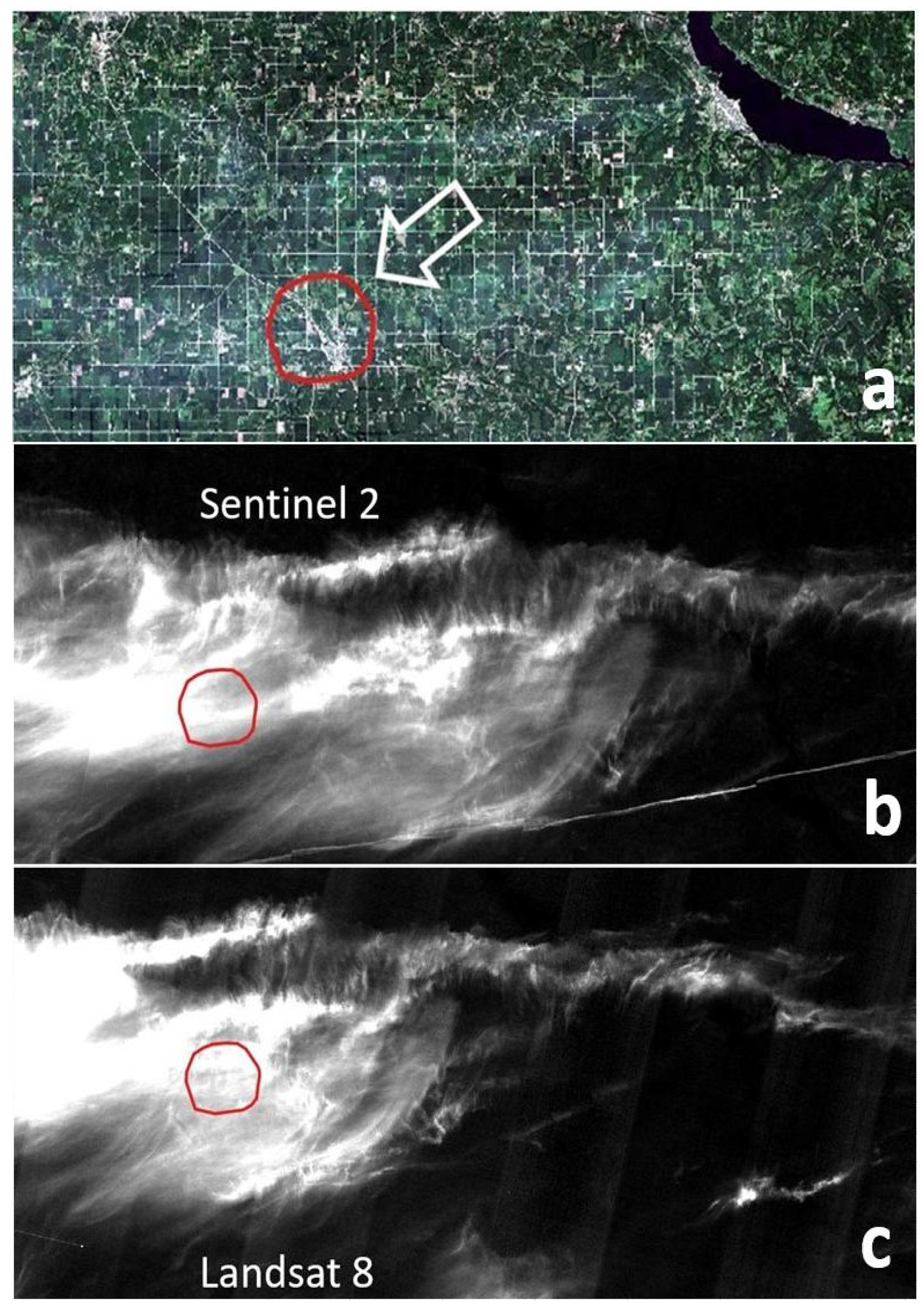
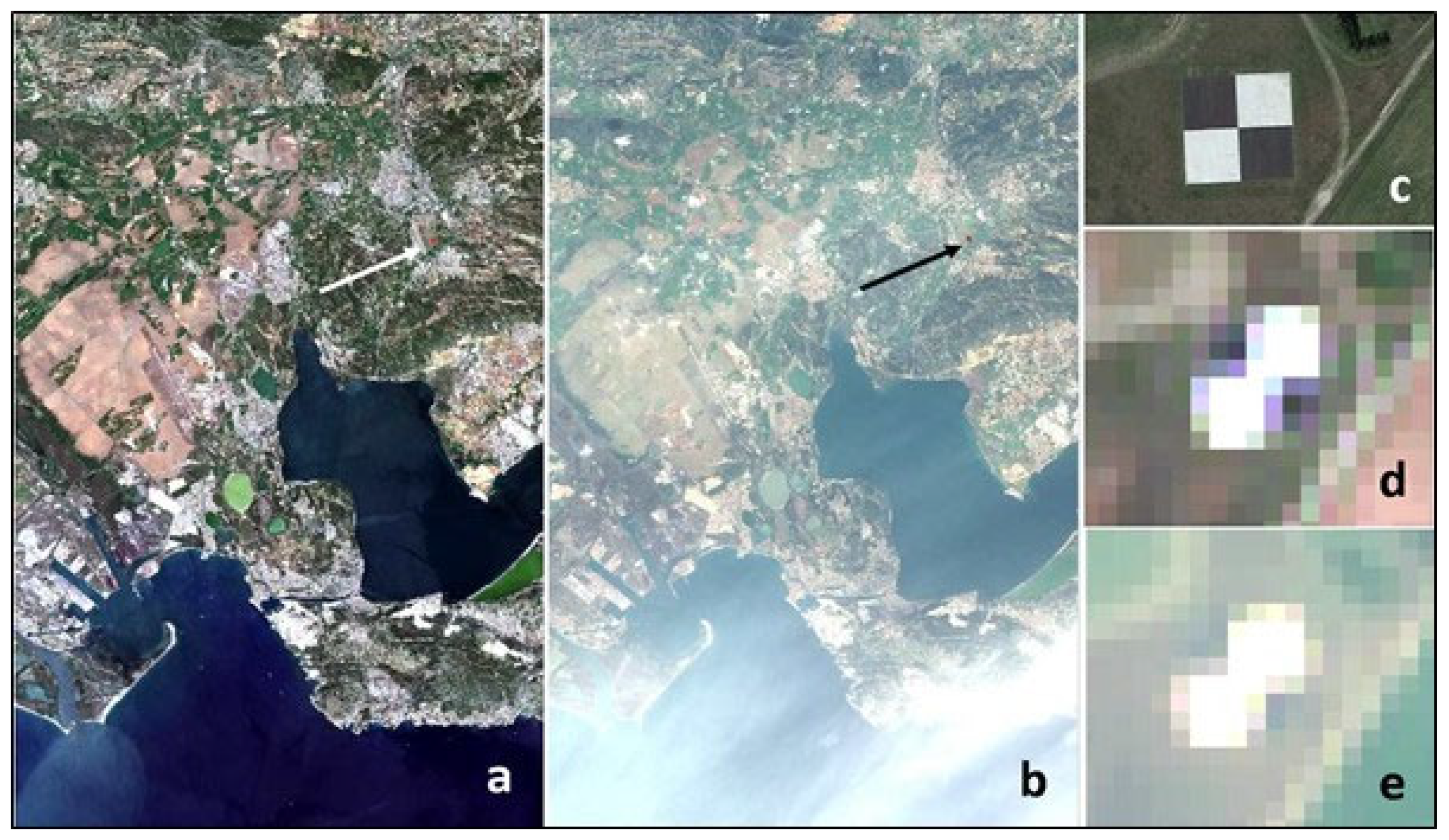
Prior to the early 1990s, simplified procedures for the retrieval of land surface reflectance factors were developed mainly from Landsat data. A summary of the methods, including radiative transfer modeling [1,2] and image-based dark object subtraction methods [3,4], were given by Moran et al. [5]. More recently, additional algorithms have been developed for multispectral atmospheric correction; Zhang et al. [6] have provided an extensive citation of AC algorithms, some based on radiative transfer modeling [7], others based on dense dark vegetation [8,9,10]. Other AC methods have used multi-temporal datasets for aerosol and surface reflectance retrievals [11,12,13]. However, such datasets are inherently unreliable because conditions may change profoundly between dataset acquisitions, as shown in Figure 1. Few of these algorithms can work in near real-time, and many are not readily automatable. Near real-time corrected image output with accuracy and precision is needed to serve the expected future massive data volume generated by smallsats.
Closed-form Method for Atmospheric Correction (CMAC) is a software package that was developed using Sentinel-2 (S2) image data specifically for application to smallsats. CMAC works in near real-time to convert top-of-atmosphere reflectance (TOAR) directly to surface reflectance, uniquely using only the statistics from the image. In contrast, automated AC methods in current use are all based upon radiative transfer (RadTran), which requires knowledge of sensor radiometry. This is problematic for smallsats that omit onboard radiometric calibration equipment to conserve weight and size. To maintain AC accuracy for any method, sensor radiometry must be updated periodically to counter changes in sensor response that are well known to degrade after launch and while in orbit [14]. Hence, for the ideal application of RadTran, sensor radiometry must be tracked for each smallsat. Also required for the RadTran workflow are ancillary data collected by other satellites for the evaluation of atmospheric conditions. Such ancillary data delays AC, thus increasing the latency of the corrected output in direct opposition to the principal value of smallsats: near real-time data for intelligence, surveillance, and reconnaissance afforded by the rapid image cadence from flocks of multiple smallsats.
Although delayed image processing due to ancillary data is problematic, a potentially greater impact may arise from frequently mismatched conditions between datasets caused by atmospheric changes in the elapsed time between image captures (Figure 1). CMAC uses only the statistics from the scene to be corrected, enabling image correction immediately upon download while eliminating correction errors arising through temporal data mismatch.
CMAC development sought a workflow that uses scene statistics for AC rather than applying ancillary data required for RadTran inputs. Examples of ancillary data include aerosol optical thickness (AOT) and water vapor from external satellites such as MODIS [15]. Current RadTran-based methods for smallsats include emulating the radiance of other research-grade satellites such as Landsat 8 and 9 (L8/9) and S2 through the use of datasets that are “harmonized” to support the vicarious calibration of smallsat radiometry [16,17,18]. Cross-calibration with harmonized datasets provides the basis for estimating smallsat sensor radiance, thereby enabling RadTran application. However, that workflow is inconvenient at least and potentially adds uncertainty.
CMAC operates in near real-time because it uses scene statistics. The accuracy and stability of CMAC version 1.1 output are examined here in relation to that of Sen2Cor, the European Space Agency’s (ESA) accepted method for S2 AC that is available as user-applied software [19]. This CMAC version was developed for AC of four-band visual VNIR data represented by S2′s blue (B02), green (B03), red (B04) and near NIR (B08a) bands.
Section 2 describes CMAC development to address the AC problem and describes the experimental design to test CMAC. Statistical testing is purposely kept simple to allow expression of the results in clearly understandable terms. Section 3 provides CMAC surface reflectance estimates in comparison to Sen2Cor. This comparison provides the context to judge CMAC accuracy, precision and limitations using both graphical and statistical data representation. The results of both methods are also compared to the uncorrected TOAR data to understand the statistical improvement provided by AC. The data are made available through extensive tables and figures in “live” spreadsheets that are downloadable through Supplementary Materials. Section 4 provides further analysis and context for a better understanding of the AC correction problem and the potential value of CMAC to serve the smallsat industry in its role of providing intelligence, surveillance, and reconnaissance. Section 5 lists five promotional aspects for AC of smallsats resulting from this paper.
2. Materials and Methods
To simplify CMAC development, Level 1C-processed images from Sentinel-2A and Sentinel-2B were considered together, as their responses were not significantly different. The quality and cadence of S2 data, every five days or less, were highly promotional for CMAC empirical testing and development.
CMAC does not differentiate among causal aerosol particles, whether due to smoke, dust, thin clouds, etc., but instead corrects imagery according to the output from an atmospheric index model that is mapped directly from each image’s spectral band responses. Aerosol particles are the dominant atmospheric effect resulting in the change from VNIR surface reflectance to the TOAR measured by the satellite [20]. While water vapor is another significant variable that affects atmospheric light transmission, the visible spectral bands are well known to be free of effects from water vapor influences [21], and the S2 NIR B8A in CMAC v1.1 is positioned to avoid water vapor absorption [22]. The B8A has 20 m pixel spatial resolution, while the visible bands have 10 m resolution. This difference has posed no problems for correction or for applications; however, hypothetically, the higher the resolution, the better CMAC can accurately estimate true target surface reflectance because of less reflectance mixing and finer differentiation of atmospheric effects.
2.1. Developing an Atmospheric Index, Atm-I, to Scale the Correction
The VNIR atmospheric effect in imagery is treated in CMAC as a single lump-sum variable. TOAR band statistics are measured across each image within discrete non-overlapping square grid cells. An atmospheric index, Atm-I, is calculated for the S2 blue band (B02) based on VNIR band statistics. This approach resulted from the choice of vegetation as a reference against which atmospheric image effects could be measured. Vegetation is also used as a reference for MODIS, S2 and Landsat as “dense dark vegetation” (DDV) to assess atmospheric aerosol content pursuant to AC application [23]. B02 was selected for Atm-I rather than the shorter-wavelength coastal aerosol band, B01, which saturates at much lower levels of visible haze, thus limiting the potential range for AC. Further reference to the S2 blue band is made specifically to B02.
Development of a statistical model to assess Atm-I as a scalar for CMAC AC began with spectral measurements of continuous DDV plant canopies using an ASD field spectrometer. These data were normalized to S2 responses using the published relative spectral responses for each band [19]. Test applications of this surface reflectance reference measured the lowest non-water blue band values discriminated by NIR threshold in grid cells arrayed across images dominated by DDV from the Amazon Basin and the intensive mechanized farming of the American Midwest. This testing confirmed that a workflow employing vegetation as a surface reflectance reference can produce highly sensitive grayscale maps that emulate visible haze. The remarkable stability of blue reflectance across many plant species is a product of physiologic mechanisms that optimize photosynthesis. Plant carotenoid pigments permit the absorbance of blue light for photosynthesis safely across a range of insolation from shade or cloudy days while avoiding damage during cloudless summer days by dissipating the excess energy as heat [24,25,26]. Against this known surface reflectance, the atmospheric effect can be readily estimated as the increased reflectance due to backscatter.
Though proving to be an excellent reference for measuring atmospheric effect, a method based solely on vegetation would restrict application only to areas where such plant cover is present [27]. However, DDV can also provide the means to train a predictive statistical model to assess atmospheric effects based solely on scene statistics, regardless of the surface conditions or presence of DDV. The following workflow was used to establish a model to measure the atmospheric effect of images spatially in the form of a single index, Atm-I, from the spectral responses of the four VNIR bands included on virtually all optical smallsats. Translating the vegetation reference would require an enormous amount of ground truth data that did not exist; however, by assuming the surface reflectance of a calibrated vegetation type, Atm-I model development could proceed. Model development was also enabled through the quality, cadence, and resolution of the S2 data. Standardization of the surface reflectance of cultivated crops to serve as DDV provided the means to assume the surface reflectance of target DDV identified on S2 images for model calibration. This workflow proceeded through the following steps:
- (1)
- ASD spectrometer measurements of cultivated crops demonstrated consistent surface reflectance usable as a surrogate blue surface reflectance for the crop when identified in imagery.
- (2)
- A DDV target crop, alfalfa, was adopted as a surrogate estimator of surface reflectance when found in healthy closed canopies. Alfalfa was chosen specifically because it is commonly grown under both irrigated and rainfed conditions. This offered the opportunity to measure spectral responses from DDV index plots and adjacent subplots of variable cover ranging from sparse desert through full DDV expression in humid climates.
- (3)
- Numerous S2 images obtained within two months of summer solstice were assembled that contained the target crop in arid to humid climates and across a range of atmospheric conditions from clear to hazy. The sampling period was chosen to reduce solar zenith angle effects.
- (4)
- One or more AOIs were chosen for each image that appeared clearly. For AOIs where haze was present, such haze was examined to assure that it was expressed evenly across the AOI.
- (5)
- AOIs were chosen to contain an index plot of the most vigorous expression of the alfalfa crop identified through examination of TOAR NDVI. Such plots were chosen as the index samples to serve as the dependent variable that would represent Atm-I.
- (6)
- Subplots of homogeneous cover were chosen around each index plot to represent various levels of vegetation response ranging from bare ground to DDV across many AOIs set in widely divergent environments.
- (7)
- The extent of each AOI containing index plots and subplots was restricted to within a diameter of about 5 km to further control variation in Atm-I.
- (8)
- Values of the four VNIR spectral bands were extracted from the index plots and associated subplots characterized through their maximum, minimum, and median values.
- (9)
- The lowest consistent TOAR blue band values of the target crop were chosen to represent the surrogate Atm-I of the index plots.
- (10)
- The extracted VNIR spectral data from the index plots and their associated subplots were pooled and then modeled by multiple linear regression and assuming a negative binomial distribution. Model iterations were tested to determine the best data combinations to predict the surrogate Atm-I blue band TOAR of the index plots from the paired TOAR spectral data.
- (11)
- The blue and red band reflectance levels were found to be highly significant for the model function, while the green and NIR bands were found to add little. The minimum values for the red and blue bands were chosen as the inputs to the final Atm-I model. Since a binomial distribution was assumed, the estimated value from the Atm-I model was based on a logarithmic scale; the estimated Atm-I level was obtained by applying the exponential function to the model value.
Application of the Atm-I model is made using a non-overlapping grid to select the lowest values of the red and blue bands in each grid cell. The output forms a grayscale, with the brightness constituting the scalar Atm-I levels needed for e AC of the image. Minor smoothing is applied to the Atm-I grayscale image to control pixelation effects due to abrupt changes in estimated Atm-I levels between grid cells. An example Atm-I grayscale output is shown in Figure 2.
The Atm-I model was confirmed by comparison to observable patterns in the grayscale output for images with significant haze mapped using the pattern of blue reflectance over continuous areas of DDV (Figure 2). Because the Atm-I model works directly with the red and blue band responses across the scene, it produces a surrogate spatial estimate for what direct application of dark vegetation would produce were it present in the image. No attempt was made to interrelate Atm-I output to a similar measure used to estimate aerosol particle loading, aerosol optical depth (AOD), which ranges from 0.1 for “clear” atmospheric conditions to 1.0 representing “very hazy” conditions [28] and is derived using sun photometry [29]. In the CMAC application, the Atm-I model output represents the predicted blue band reflectance from DDV and is measured as a digital number—DN (reflectance × 10,000)—that represents a correctable range from the high 700s (extremely clear) to over 1700 (features obscured in a dense haze). The abbreviation DN is used throughout to designate this rescaled reflectance.
2.2. Translating an Observation into the CMAC Equation
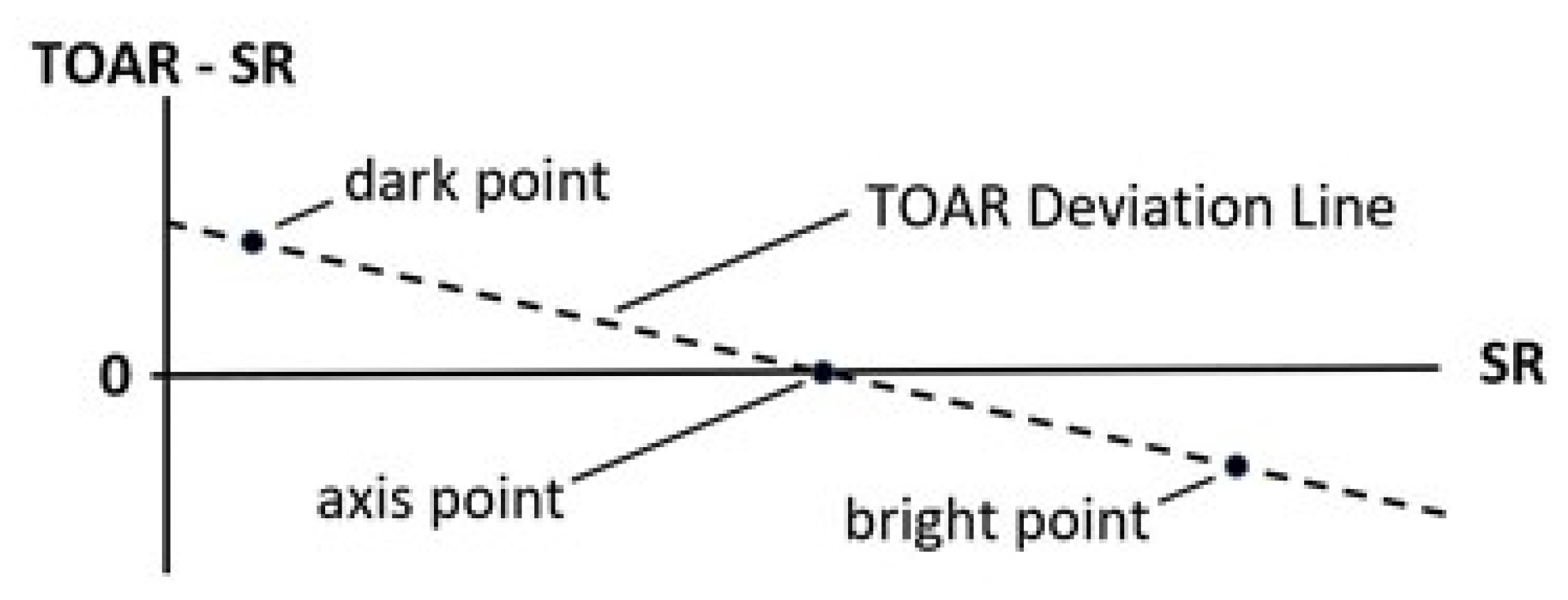
The final step in the CMAC workflow reverts TOAR to an estimate of surface reflectance by removing the atmospheric effect measured as Atm-I. This workflow is based on a graphical conceptual model representing the effect from a single Atm-I level as a line in cartesian space defined by surface reflectance and TOAR. Development of this approach began by comparing reflectance between clear and hazy conditions for a given AOI. For images with essentially the same surface reflectance, higher atmospheric aerosol increased dark reflectance from backscatter and decreased bright reflectance through attenuation. This observation was further translated into a graphic conceptual model through inversion of the empirical line method [30], which was adjusted further by placing surface reflectance in both axes (Figure 3). For a single level of Atm-I, this formulation represents the upward reflectance deviation for dark targets and the attenuation of reflectance for bright targets as a single TOAR deviation line (TDL). All VNIR bands were found to conform to this conceptual model.
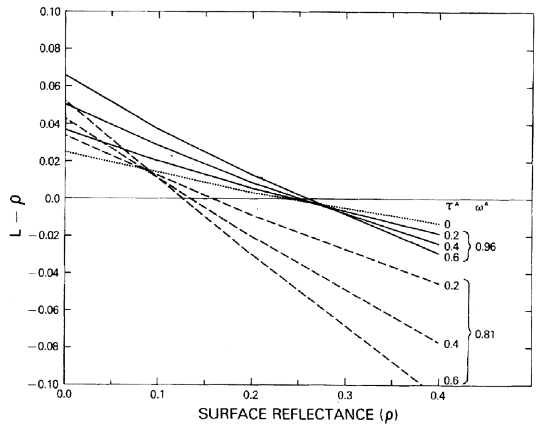
Precedence for the CMAC conceptual model can be found in Figure 2 of a paper by Fraser and Kaufmann [31] and is reproduced here in Figure 4. The linear relationships are similar to those shown in Figure 3; however, the y-axis in Figure 4 is functionally TOAR. In the context of AC, the parameter L represents radiance that necessarily includes sensor response that is the basis for RadTran applications. Including radiance complicates the calculation of surface reflectance. In the CMAC automated workflow, calibration removes the central importance of true radiance for AC.
The TDL of Figure 3 represents the deviation from surface reflectance caused by the imposed atmospheric effects measured by Atm-I. As Atm-I increases and backscatter and attenuation increase, displacing the intercept upward and steepening the slope. This conceptual model was translated into the CMAC Equation, which converts TOAR to surface reflectance for each pixel differentially across the image according to the slope (m) and the offset (b) for the TDL imposed by the overlying atmosphere. The conversion is rapid due to the efficiency of the closed-form CMAC rather than the less-efficient alternative of iteration and potentially less accurate lookup tables employed in RadTran-based methods [32,33].
CMAC Equation: SR = (TOAR − b)/(m + 1)
The conceptual model and the observations supporting it underscore that the CMAC approach rescales the TOAR to surface reflectance. These changes narrow the reflectance window, a behavior that can be measured for increasing levels of Atm-I (Figure 5). Given the behavior of reflectance to increasing atmospheric aerosol concentration, the often-used dark object subtraction method [3,4] subtracts the lowest reflectance over dark targets (e.g., water bodies) from the entire reflectance distribution. This does little to correct the reflectance distribution while introducing additional error.
2.3. Forward Scatter Effects and Calibration
Two parameters per band are needed to apply the CMAC Equation: the TDL slope and offset. Through calibration, these parameters can be predicted from Atm-I for reversing the TOAR snapshot that captured the result from atmospheric degradation of the original surface reflectance. Each smallsat spectral band requires calibration to accommodate differing sensor responses to Atm-I, thereby customizing CMAC for that smallsat’s sensor responses. A calibration target is an obvious choice for a precise and convenient establishment of the bright and dark points of the TDL, provided that special concerns are first addressed in the design of such targets.
Through R&D analyses, an additional atmospheric phenomenon became apparent that results from the interactive effects of ground-target reflectance and atmospheric aerosol particles. As Atm-I increases, the higher reflective energy of bright targets illuminates aerosols from below, thus brightening and scattering the Atm-I responses captured by the imager. This phenomenon affects the relationship of slope and offset for the application of the CMAC Equation and may prevent the use of existing targets that combine adjacent dark and bright panels in a checkerboard pattern (Figure 6). Due to forward scatter effects, such checkerboard targets can provide measurable TOAR only when (1) employed under the cleanest of atmospheric conditions, (2) the panels are physically separated, and (3) the panels are large in relation to the imager’s spatial resolution. Forward scatter affects calibration curves beyond what is captured by the conceptual model in Figure 3; fortunately, this can be accounted for intrinsically through calibration.
An appropriate calibration target with accompanying precise and recently measured ground truth was not available; therefore, to provide for CMAC development, slope and offset were calibrated vicariously through image comparisons between clear and hazy conditions, with additional guidance from ground truth data collected by ASD field spectrometer. CMAC results for this calibration compared well with Sen2Cor results developed for the same images. This low Atm-I calibration was then adjusted sequentially for higher Atm-I by matching the surface reflectance estimates of the higher to the lower Atm-I image through the selection of appropriate slopes and offsets. The slopes and offsets derived in this manner were recorded for each measured Atm-I on multiple clear to hazy images to establish the calibration relationships for surface reflectance estimation across the range of Atm-I that can be encountered operationally.
During previous method proofing, CMAC v1.1 was tested on multiple Sentinel 2 images from diverse environments that included low spectral diversity such as oceans and deserts as well as images degraded from haze due to smoke, fog and, to a more limited extent, dust. CMAC was found to correct all images and remove profound levels of haze, thus demonstrating applicability in all environments and at least to first order, doing so irrespective of aerosol type. This testing also indicated that the corrected VNIR bands are correct relationally and therefore represent close estimates of surface reflectance.
To verify the mathematics of the correction for this investigation, CMAC v1.1 (Advanced Remote Sensing, Inc., Hartford, SD, USA) was tested against Sen2Cor v2.11 (European Space Agency, Paris, France). Performance was judged by estimation of VNIR surface reflectance for seven AOIs exhibiting consistent reflectance throughout the summer. Such AOIs were given the name “quasi invariant areas” (QIAs) in recognition of the special role they can play as targets to assess AC performance under variable atmospheric effects. QIAs provide the opportunity to objectively evaluate accuracy, stability and AC correction limits by the CMAC and Sen2Cor software. Data presented for the comparisons presented here are the output from the processing software, alone, with no other treatment except the statistical analyses documented in downloadable Excel spreadsheets (see Supplementary Materials).
While the investigation of AC here is relative to S2, a research-grade satellite that includes onboard radiometry, CMAC is applicable to smallsats without additional processing or other relationships beyond the Atm-I model and CMAC Equation. Hence, the level of accuracy achievable for AC of S2 data serves as a direct indication of the AC accuracy achievable for smallsat data.
2.4. Experimental Design: Testing CMAC against State-of-the-Art Sen2Cor
This investigation consists of two analyses to evaluate the accuracy, stability and limits for AC applications by CMAC and Sen2Cor. Analysis 1 focused on the performance of these two methods for the correction of 18 images that encompass a range of Atm-I from clear to extremely hazy of a QIA northeast of the Reno, Nevada Airport. Analysis 2 developed AC statistics for 28 visibly clear images of a Southern California (SoCal) metropolitan area within an Atm-I range expected to be more commonly encountered in operations.
Vegetation and surface wetting are two significant influences on the temporal variability of the true surface reflectance. To minimize these effects, warehouse districts dominated by flat roofs and paved interspaces were chosen as targets. Such AOIs have remarkably stable reflectance and hence form desirable QIAs because (1) the AOI boundaries can be mapped to either exclude vegetation or include minor areas of irrigated cover, and (2) the exposed flat roofs and paved surfaces assure rapid drainage and surface drying. All seven QIAs, located in regions with Mediterranean-type climates, were evaluated during June and through early August when vegetation expression was expected to be relatively static. Weather records indicate that both QIAs received no significant rainfall during multiple days before each image acquisition date.
The area of each QIA was variable but sufficiently large such that the influence upon reflectance from variations in numbers of parked cars, semi-trailers, roof repair, etc., constitute a minor stochastic variation. The smallest QIA, Highgrove in southern California with an area of about 1.5 km2, contains ~15,000 10 m pixels, and the largest, Chino, contains about 6.4 km2.
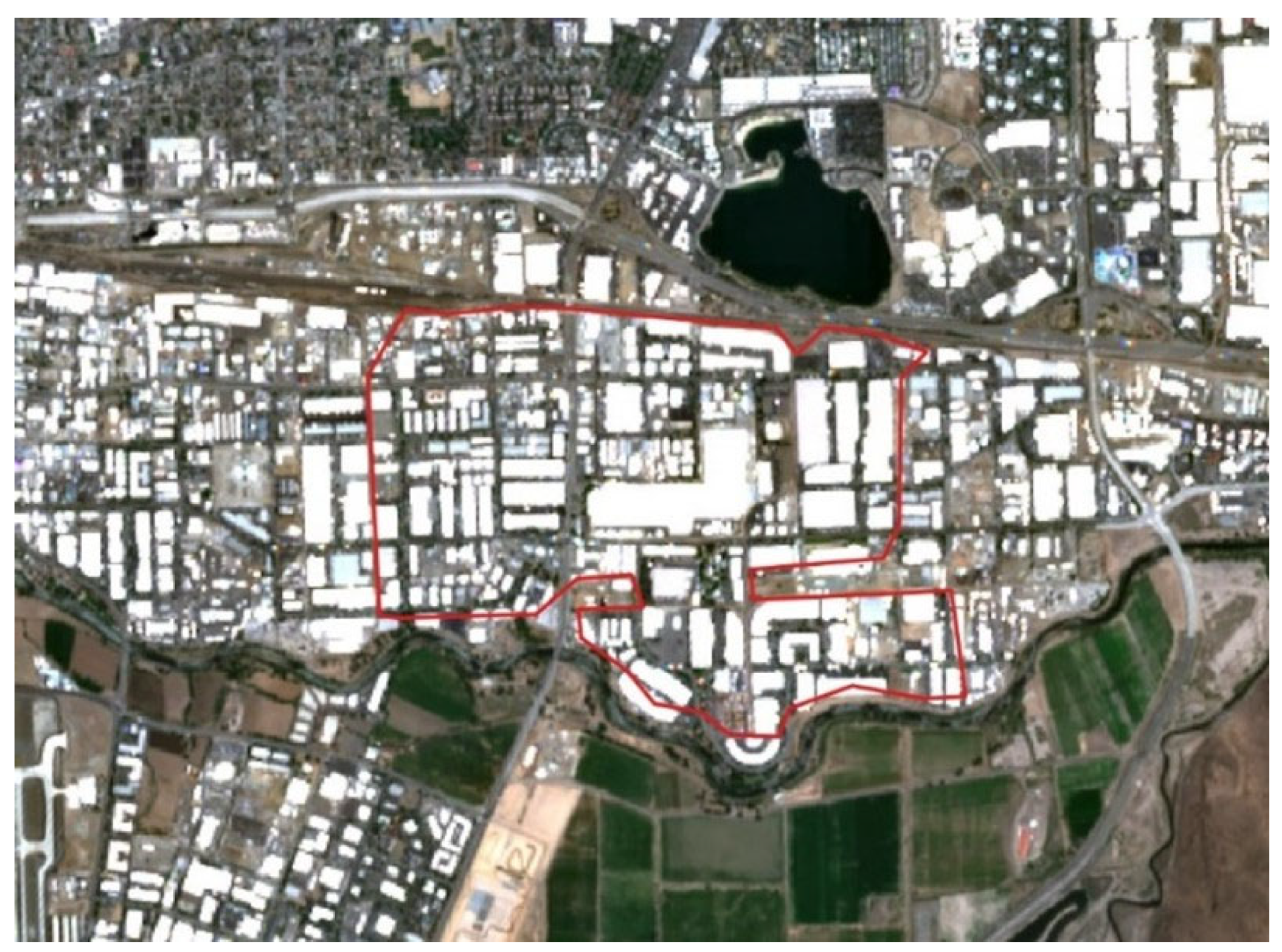
Analysis 1: The Reno QIA shown in Figure 7 is located in a sidelap region between adjacent S2 tiles, thus potentially doubling the number of overpasses otherwise available. Eighteen images were selected for analysis from June through to 22 August 2021, a period that initially captured extremely clear conditions followed by periods of intermittent, occasionally severe smoke haze from regional forest fires. The selected images were confirmed to lack cirrus cover through visual inspection of S2 B10, and the Atm-I mapped across the QIA boundaries was confirmed to be homogeneous with only minor variation, generally between two to three percent.
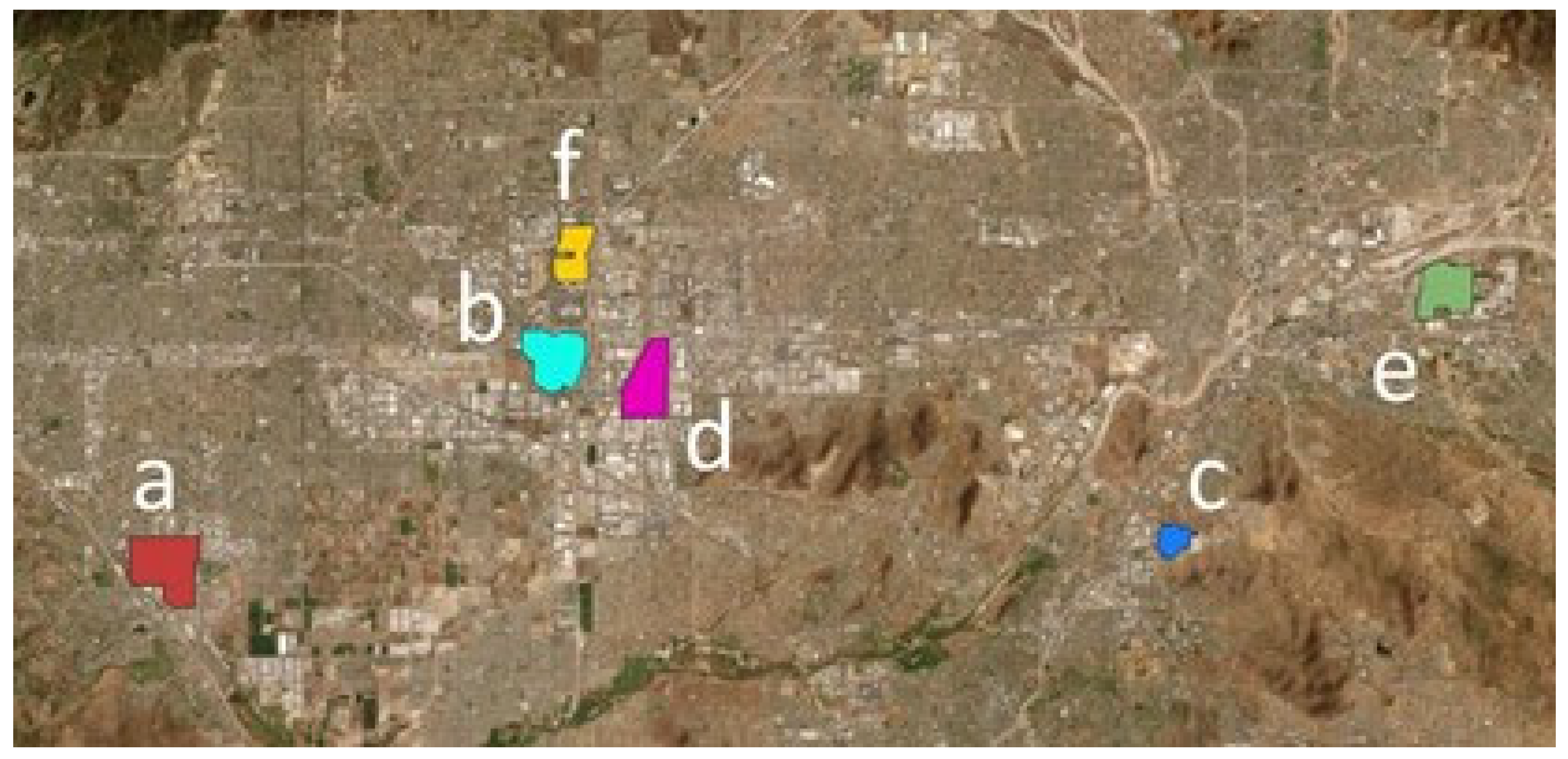
Analysis 2: Six warehouse districts were chosen in a metropolitan region of southern California east of Los Angeles covered by a single S2 tile (Figure 8 and Figure 9). Twenty-eight S2 images were selected that met two criteria: (1) collection in June through early August in 2020, 2021 and 2022; and (2) lacking cloud cover, including cirrus determined through visual inspection of S2 band B10. The images exhibited no visibly discernible haze.
The restriction for the collection period to about three months controlled for reflectance changes of senescing unirrigated weedy plants and restricted the solar zenith angle (SZA) to remain within five degrees of the minimal angle around the summer solstice. These AOIs were accepted as QIAs, and polygons were drawn around each to exclude vacant land and non-irrigated plant cover. Among the 28 images selected, eleven were from 2020, eight were from 2021 and nine were from 2022. This provided 168 separate Atm-I levels for comparison when viewed across the six AOIs (6 QIAs × 28 images). Though the six QIAs are in the same region, measured Atm-I varied among the QIAs even on the same day.
2.5. Data Analysis
CMAC and Sen2Cor corrections were run for the area within each QIA polygon for each image tile. Pixel values were extracted for the four VNIR bands from each QIA for three treatments: TOAR, CMAC-corrected and Sen2Cor-corrected. To provide easy-to-follow documentation, all statistical analyses were performed in Excel spreadsheets. For both analyses, statistical distributions for these treatments were recorded, by band, for each image as cumulative percentiles starting at 0.1, 1, 3 and 5, then continuing in five-percentile increments to the cumulative reflectance at the 95th percentile. The suite of 22 separate statistics for each QIA permitted assessment of AC performance across the range from dark to bright reflectance. Statistical analyses were treated separately for each QIA because the reflectance within each QIA was internally consistent, but variable compared to the other QIAs. Statistical dispersion (therefore, also its antonym, precision) was evaluated for each QIA dataset using the coefficient of variation expressed as a percent (CV%) and calculated from the ratio of standard deviation to the mean for the suite of 28 images.
Estimation error was evaluated for Analysis 2 in an initial step assessed per QIA by averaging the percentile-wise values of the three lowest Atm-I images. The resulting averages per QIA were treated as the standard to estimate error for each percentile of each image within that QIA according to
% error = 100 × (value − standard)/standard
The resulting values of % error for each band were then pooled from the six QIAs to evaluate error statistics for the operational range of Atm-I and from dark to bright reflectance for both CMAC and Sen2Cor. These error statistics were tracked for each cumulative percentile for each image and were included in the pooled sample that was then ranked from low to high to provide for graphical assessment of CMAC and Sen2Cor error distribution. The pooled sample resulted in suites of n = 3696 (6 QIAs × 28 images × 22 percentiles) error estimates for each band of both treatments.
Data extracted from the 46 total S2 images were exported to and analyzed in Excel spreadsheets where figures were generated. A list of these images is presented in Appendix A. All Atm-I data quoted in this paper are median values for the region within each QIA boundary. The data presented in this section are excerpted from over 4000 individual extracted median estimates of surface reflectance from 22 cumulative percentile steps of the reflectance distributions for each of three treatments: TOAR, CMAC and Sen2Cor. These data were examined for the 18 images of the Reno QIA (Analysis 1) and the 28 images of the six Southern California QIAs (Analysis 2).
The workflow for this assessment was comprised of the following steps: (1) clipping the Atm-I, TOAR, Sen2Cor, and CMAC-corrected image bands from the image tiles to each QIA boundary and extracting the median statistics from the clipped areas; (2) aggregating the treatment data for each QIA, sorting it by band and in order of increasing Atm-I; (3) generating Excel spreadsheets containing the aggregated data and (4) analyzing the spreadsheet data within Excel to generate the summary plots and tables. The interested reader is invited to download the Excel data analysis spreadsheets that are available in Supplementary Materials and to test correct 4-band VNIR Sentinel 2 images using the S2 Cloud Pipeline. Instructions for access are given in Supplementary Materials.
3. Results
On a desktop PC (64 MB Ram, Windows 10, C++-based code), CMAC corrected the four VNIR bands of full S2 image tiles (~120 million image pixels) in an average of 91 s. The python-based desktop Sen2Cor processed the same tiles in an average of about 20 min, though for the 13 bands included in S2 “.SAFE” image packages.
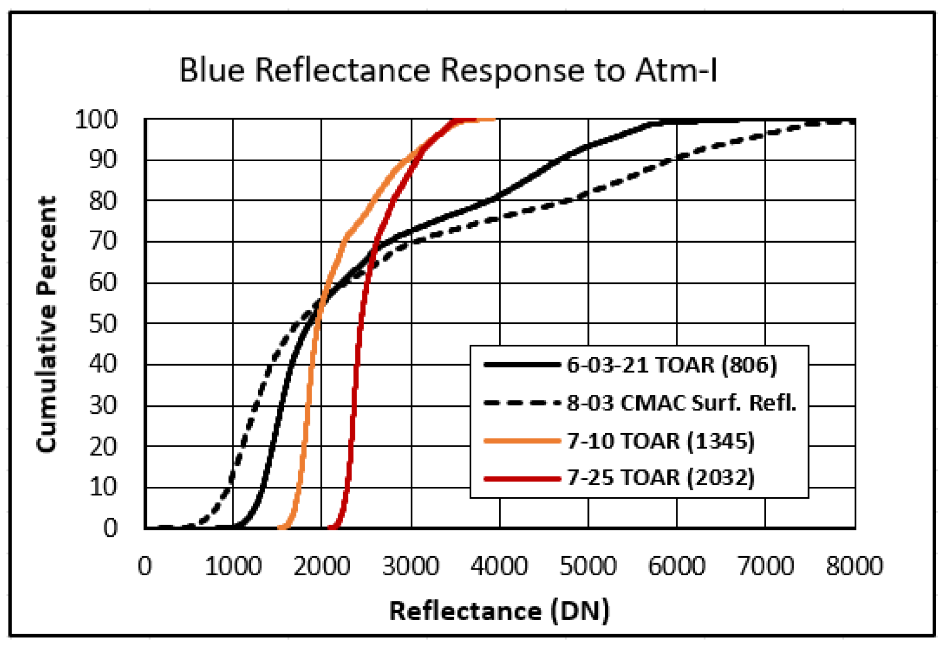
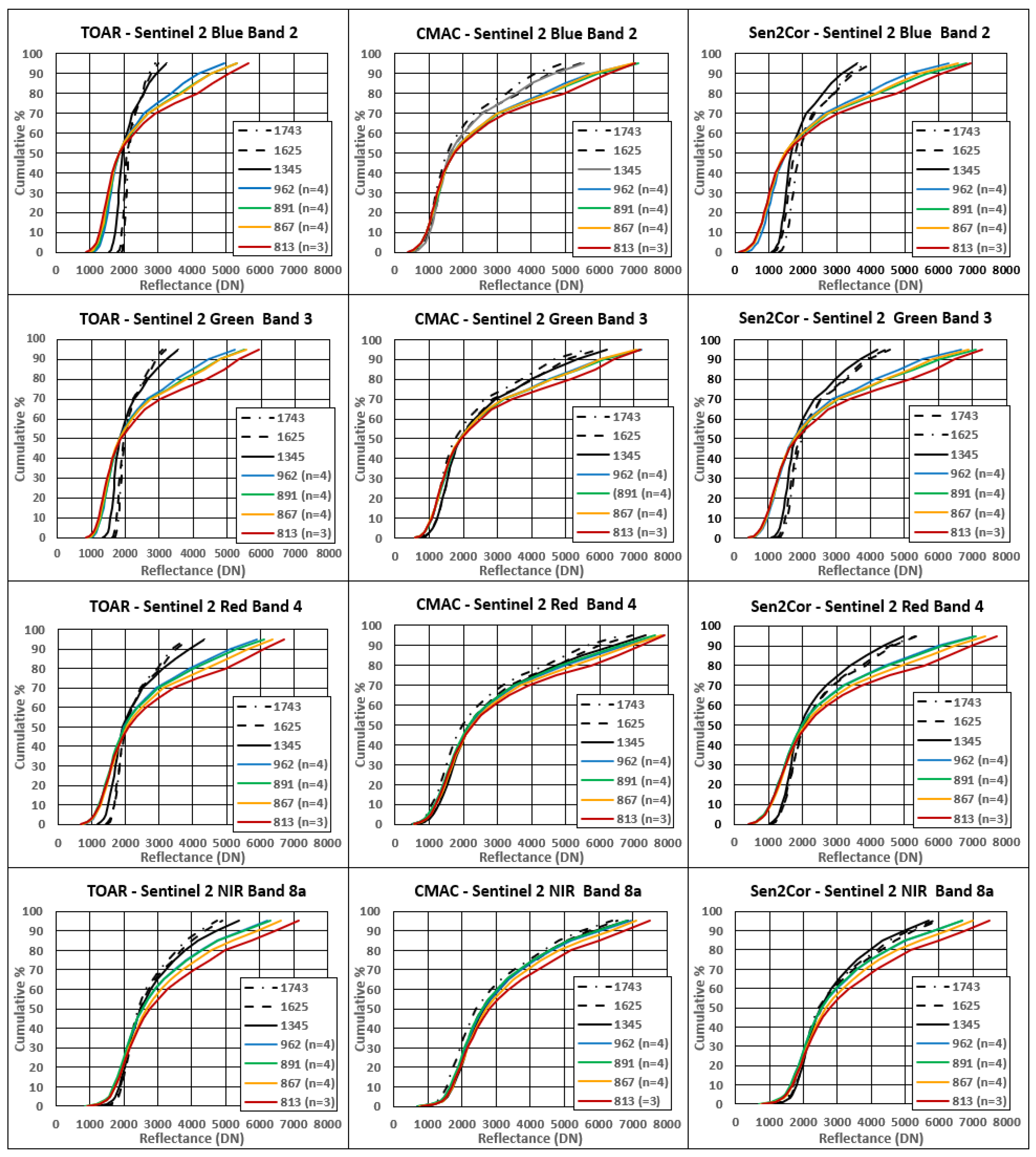
Analysis 1: Reno QIA statistics were extracted and analyzed from eighteen images. A summary table presented for the Reno QIA available in the Supplementary Materials provides CV% values that are noticeably elevated above CV% for Analysis 2, also available in the Supplementary Materials. This was due to the inclusion of three high Atm-I images that proved challenging for both methods. This conclusion can also be reached through the examination of Figure 10 in which seven curves are plotted showing the trend in correction as judged by Atm-I from unusually clean atmospheric conditions to the extreme haze from wildfire smoke. Scatter increased with Atm-I. To reduce the number of curves for clarification of trends responding to increasing Atm-I, data of similar Atm-I ranges were averaged (n = 3 or n = 4) for each percentile of reflectance within each treatment. Sen2Cor can be observed to fail at Atm-I levels of around 1345 and above. Data from the three extreme Atm-I images also show increased CMAC CV% as indicated in Figure 10 by the slight deviation from the statistical weight of the curves generated by results for Atm-I levels of 962 DN and lower. These calculations and the complete dataset are available for “Reno.xlsx” through a link in Supplementary Materials.
As shown in Figure 10, CMAC surface reflectance estimates are roughly commensurate with Sen2Cor for images with lower Atm-I—these curves are displayed in color. The average of the three unusually clear images with the lowest average Atm-I (813) displayed in red was taken to be the best “surrogate” approximation of true surface reflectance. Above Atm-I levels of approximately 2000 DN, the CMAC AC curves significantly diverge above the corresponding surrogate surface reflectance curves. However, this represents a net decrease in estimated surface reflectance.
Though CMAC and Sen2Cor AC methods are very different, both captured the trend of decreasing bright reflectance at higher Atm-I levels. Hypothetically, this divergence indicates an atmospheric phenomenon of diffuse shading by aerosol particles that reduces TOAR reflectance. As the CMAC Equation predicts, this results in a lower surface reflectance estimate. This divergence is systematic, so it can potentially be adjusted by empirically fitted relationships for each band if the estimation of the true surface reflectance for brighter targets is desired and the added processing time is not problematic. As discussed later, the true reflectance of bright targets may not be of direct interest for most analyses.
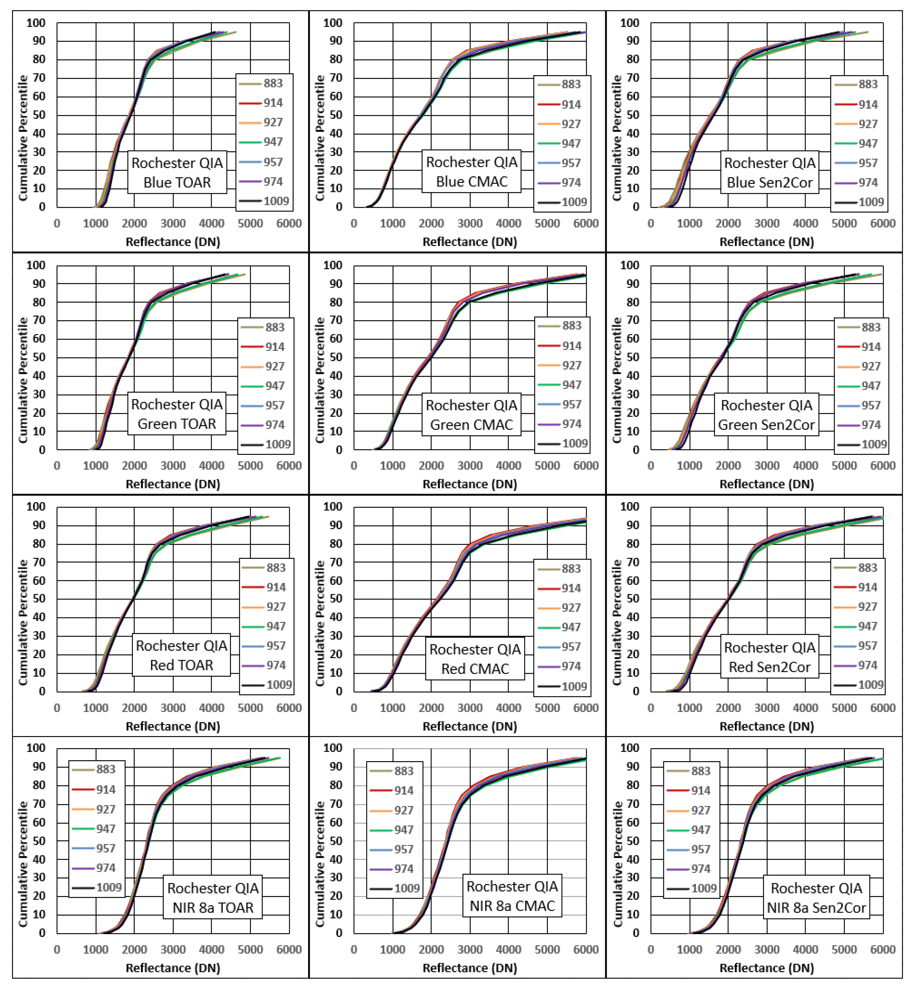
Analysis 2: The six SoCal QIAs were evaluated to test AC performance within an Atm-I range expected to be encountered in typical operation. Figure 11 presents seven curves derived for the Rochester QIA, each being an n = 4 average calculated from within similar Atm-I ranges.
As previously mentioned, each of the 28 images analyzed for the SoCal QIAs appeared visually clear across the entire range of median Atm-I recorded for the images. Of the 168 unique image-QIA combinations, only four images exceeded an Atm-I of 1050 DN, and those by less than 17 DN. Summary tables for the statistics are presented in for the six QIAs available through a link in Supplementary Materials. The precision of the curves in the Figure 11 example QIA is indicated by how tightly the curves plot and is comparatively better for the suite of SoCal QIAs due to the more expected dynamic range of Atm-I in contrast to the Reno QIA analysis, which included three extremely hazy images. From the analysis of hundreds of images, most atmospheric correction is performed within an approximate Atm-I range of 800 to 1050 DN. We have observed alarming exceptions that occurred during recent summers in the United States from the west coast to the Great Lakes region due to wildfires in Canada and the western United States that drove Atm-I imagery above 1050 DN over millions of hectares of farmed land for extended periods, adversely impacting image uses for precision agriculture and other applications.
CMAC’s high accuracy in the lower limb of visible-band surface reflectance, generally less than about 2000 DN, is crucial for precision agriculture and AI feature extraction because these darker features define the analytics of interest in vegetation indices and in prominent observable features [34,35,36]. The suite of 12 curves as shown in Figure 11 is provided in Excel spreadsheets for each of the six SoCal QIAs are available through the link in Supplementary Materials.
3.1. Precision
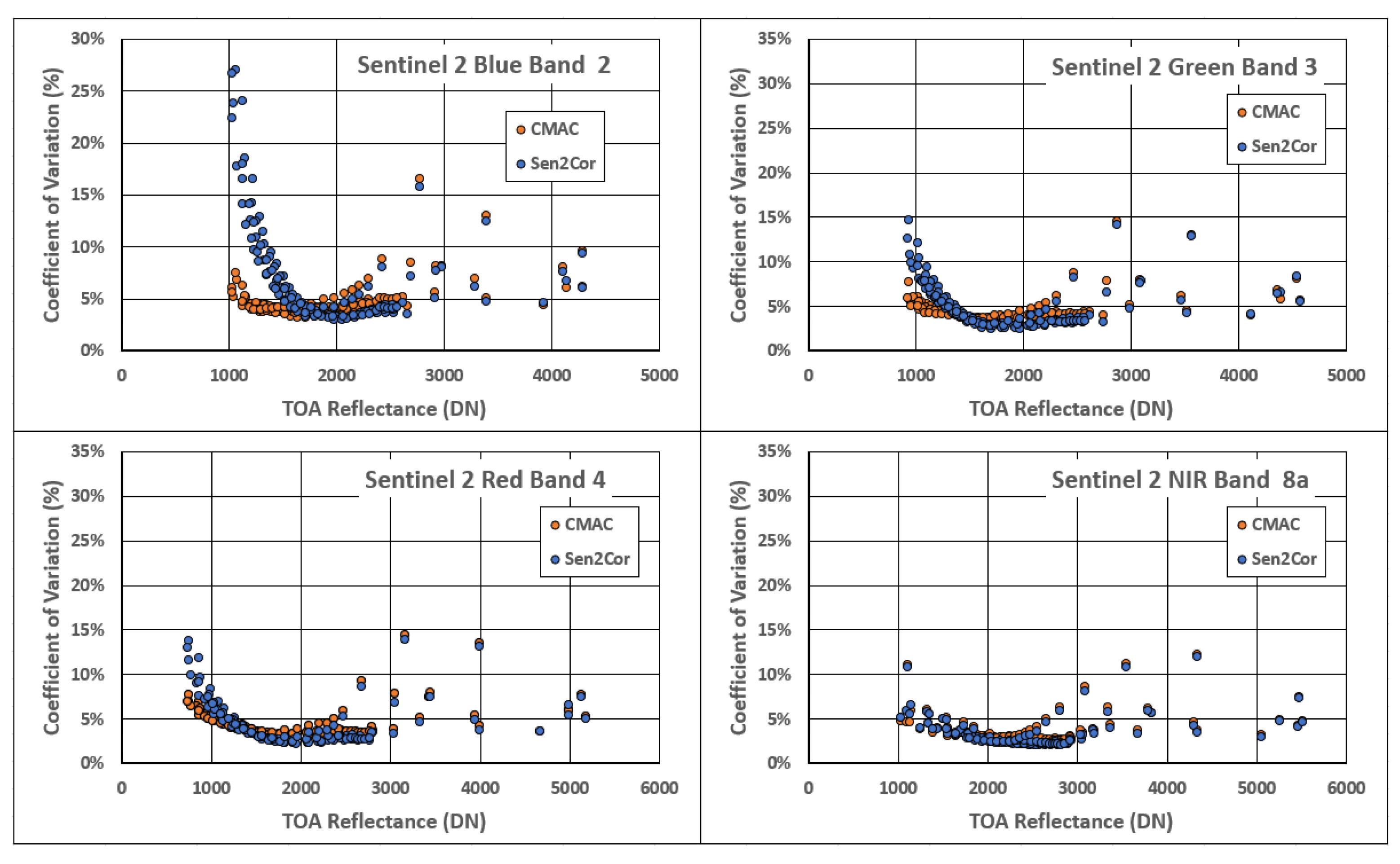
Bandwise average CV% for all 28 images and for each of the 22 cumulative percentile steps of the six SoCal QIAs were combined into one dataset to examine how precision is affected by increasing reflectance for both CMAC and Sen2Cor output (in Supplementary Materials as “SoCalCV%.xlsx”). These cumulative percentile-step averages were plotted against TOAR to represent the unbiased trend from low to high reflectance for both methods (Figure 12).
The resulting pattern of bandwise CV% is instructive. Moving rightward from the origin toward higher TOAR, CV% is initially high, decreases to a trough and then increases in a quadratic-like manner. This behavior is exhibited in all four bands for both CMAC and Sen2Cor despite very different workflows and data inputs. This result provides support that the CMAC conceptual model, as expressed in Figure 3 with its teeter-totter-like TDL response, correctly portrays the phenomenology of atmospheric aerosol effects. According to the CMAC model, the greatest precision is expected to occur at the axis point where the TDL crosses the x-axis and the affected image’s surface and TOAR are equivalent. The statistical distribution in the region around the axis point will, therefore, tend to have minimal scatter. It should be noted, however, that the axis point is a concept and not a fixed value. The axis point migrates rightward as Atm-I increases; hypothetically, this trend is caused by forward scatter.
In Figure 12 the trend in CV% can be seen to increase above a scaled TOAR reflectance level roughly between 2300 to 2800 DN depending upon band and method, but the values become widely spaced and, for each dataset, highly scattered. Uncertainty increases at higher reflectance, as can be seen in the spreadsheets and tables that summarize the QIA CV% data available through the link supplied in the Supplementary Materials.
3.2. Estimation Error
As noted in Figure 10, AC results for the lowest Atm-I (clear) images are expected to be closest to true surface reflectance since the correction requires minimal adjustment for its estimation. An assumption that the surface reflectance estimates of CMAC and Sen2Cor for low Atm-I images are surrogates for true surface reflectance offers a means to examine the propagation of error in each AC method. Following this logic, % error was estimated using the average of the three lowest Atm-I images for the 28 images of each SoCal QIA and used as surrogate true surface reflectance values. These calculations were made per the 22 cumulative percentile steps so that the statistical examination could further define the relationship of the error to reflectance brightness.
Because each of the QIAs was chosen for its quasi-invariant reflectance, AC results for the collection of QIA images are expected to yield reflectance values that remain similarly invariant. Examination of the values for each image indicated that there was no apparent relationship with time for either method. For CMAC, there was also no striking relationship for the magnitude of surface reflectance estimates with Atm-I. For Sen2Cor, however, a trend for surface reflectance error increasing as Atm-I increased was readily discernable.
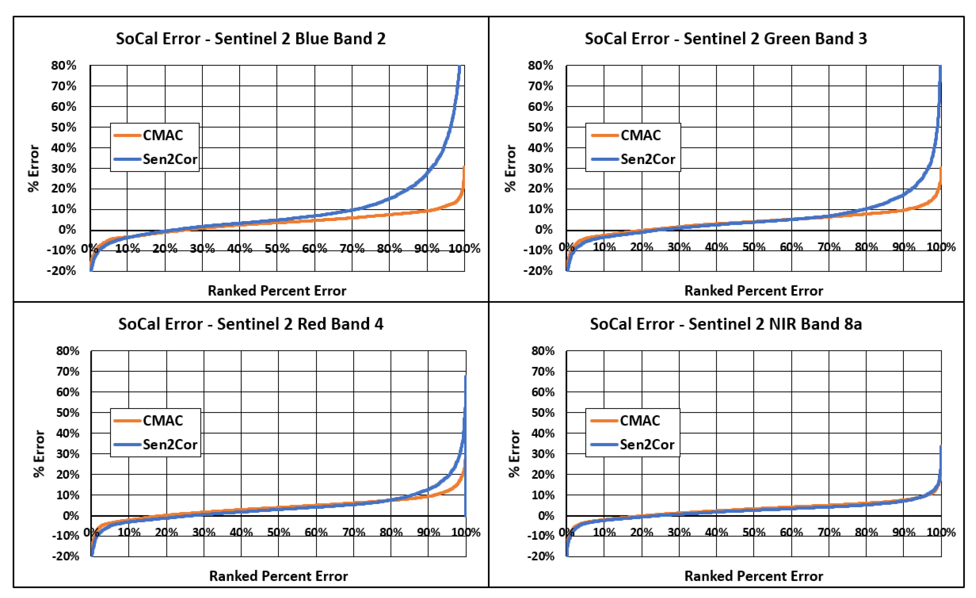
Error estimates were calculated for CMAC and Sen2Cor for each QIA from their individual surrogate true surface reflectance (CMAC with CMAC, Sen2Cor with Sen2Cor). The values for all six QIAs were combined to robustly represent the error distribution for each band (n = 3696: 6 QIAs × 28 images × 22 percentiles). The error estimates were ranked from lowest (under-estimation error) to highest (over-estimation error) and plotted to compare CMAC to Sen2Cor per band for the entire SoCal dataset (Figure 13). These calculations, as well as the trend in the data output, can be traced in the individual downloadable QIA spreadsheets that fed statistics to the downloadable available in Supplementary Materials as “SoCal%Error.xlsx”.
The ranked percent error curves for CMAC and Sen2Cor in Figure 13 agreed well through most of the bandwise % error distributions with the notable exception for the higher ranked values in the visible bands. The under-estimation error was well-constrained and roughly equivalent between the two methods. The upward deviating curves represent an over-estimation error that was much greater for Sen2Cor, especially at shorter band wavelengths—the blue band was more severely affected than the green band. The estimated error was the lowest for NIR 8A.
Over-estimation of visible-band reflectance in Figure 13 was confirmed to be the origin of the greater statistical dispersion of low reflectance observed in the plots of Figure 11 and in the CV% tables and the “raw data” across the six Excel files available through Supplementary Materials. The data in the summary tables show this trend but under-represent the severity of Sen2Cor instability at higher Atm-I because the most widely divergent values were masked by averaging with the majority of comparatively low Atm-I images in the larger image pool. Some Sen2Cor CV% values exceeded 100% for individual images with higher Atm-I, a trend that can be seen in the individual downloadable QIA spreadsheets. The trend for overestimation errors in visible bands is evident in Figure 13 for Sen2Cor. This can be viewed as instability. In contrast to visible bands, NIR 8A error estimates by CMAC and Sen2Cor closely agree.
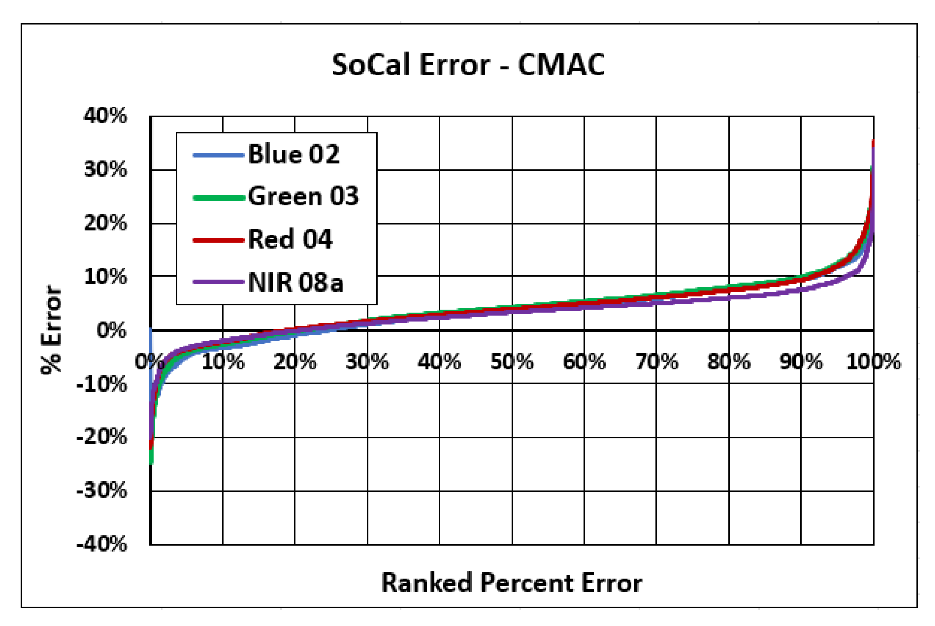
The CMAC % error curves have roughly equivalent shapes and magnitudes. In Figure 14, the estimates for the visible bands plot nearly atop one another. The agreement of CMAC error curves indicates greater stability in VNIR band correction.
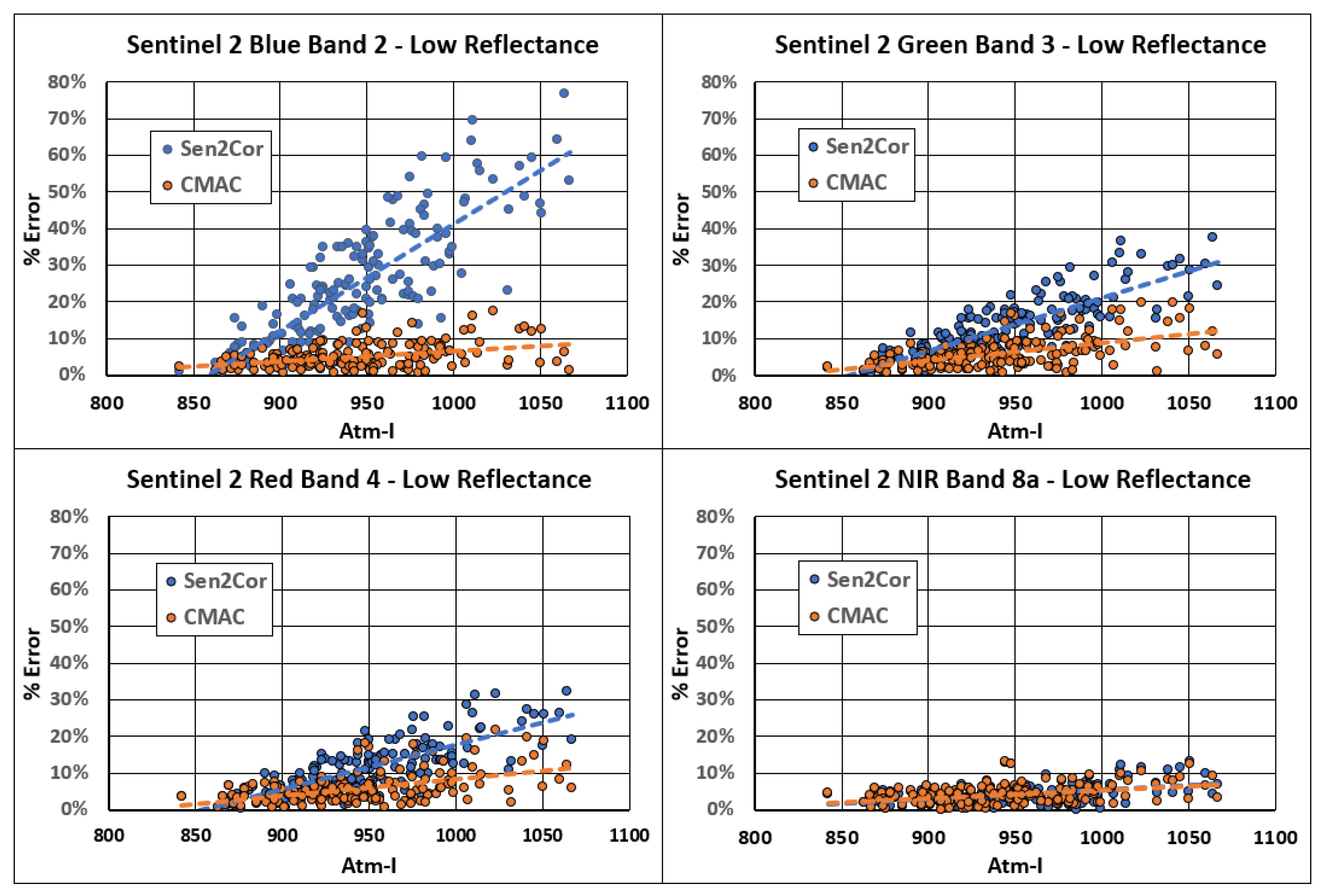
Toward understanding the range of Atm-I that can be corrected accurately by both methods, the low, dark end of reflectance was explored further using averages of the low reflectance % error values as an index to compare to the median QIA Atm-I measured for each image. For this final test, the absolute values of percent error were averaged for the 0.1, 1, 3, 5, 10, 15 and 20th percentiles to form an index, one per image, to compare to the range of the recorded median image Atm-I. The % error values were combined for all six QIAs and plotted (Figure 15). The corresponding reflectance range encompasses up to 2000 DN for NIR 8a and about 1000 to 1200 DN for visible bands. These calculations can be viewed in Supplementary Materials as “SoCalLowRefl%ErrorDistr.xlsx”.
Because the suite of 28 images for each QIA expressed different Atm-I values, the test in Figure 15 provided 168 unique independent values for comparison to the low reflectance % error index in each band. To place the low reflectance measured over the SoCal QIAs into context, the reflectance level for the visible bands measured at the 0.1 cumulative percentile for five of the six QIAs corresponds to the approximate reflectance typical of the dense dark vegetation used to calibrate the Atm-I model. Hence, a percentile range from 0.1% to 20% is considered to be a valid range for examination of how the low reflectance limb of the surface reflectance distribution is impacted by an error that would affect image utility whether for precision agriculture or AI feature extraction.
Figure 15 illustrates a marked decrease in Sen2Cor’s visible band stability as Atm-I increases above about 900 DN. CMAC exhibits a much shallower error trend as Atm-I increases, starting at an Atm-I level of approximately 850 DN. Figure 15 demonstrates that CMAC outperforms Sen2Cor accuracy for AC in the low reflectance portion of visible bands for the most common range of Atm-I that will be encountered in routine AC. As noted in Figure 10, CMAC can still provide useful results even at “extreme” levels of Atm-I exceeding 1700 DN, well beyond the atmospheric effects that can be corrected by Sen2Cor. These graphics form a milestone for judging future R&D efforts to enhance CMAC accuracy.
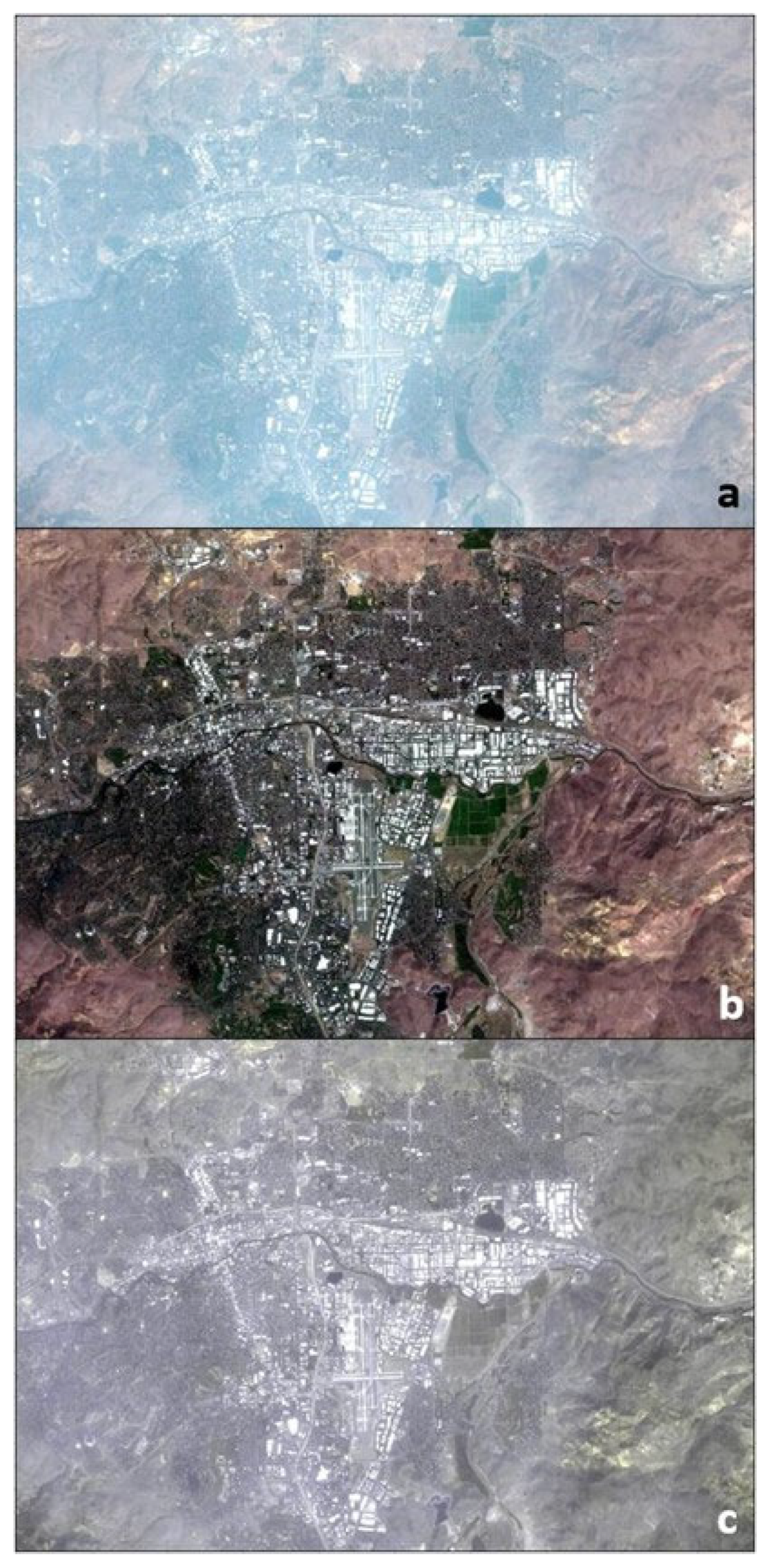
As mentioned earlier, CMAC v1.1 has been tested on images from diverse environments around the Earth. While these tests demonstrate that CMAC can clear images with profound haze, there has been no direct means to confirm that the cleared images represent true surface reflectance. The data developed for this investigation have provided such direct confirmation. Returning to Figure 10, the most extreme image haze evaluated in this paper, graphed for the Atm-I = 1743 image, also provided results close to surrogate surface reflectance that was confirmed to provide image clearing (Figure 16). Hence, when corrected by CMAC, images that have heavy haze cleared from the image can provide results that are close to the true surface reflectance. This is a valuable result that will help push the upper limit of correction to even higher Atm-I levels.
4. Discussion
Smallsats are unequivocally the future for remote sensing intelligence, surveillance and reconnaissance (ISR) applications. CMAC was developed to support this mission by enabling smallsat AC to be independent of ancillary data and operate in near real-time. Because CMAC correction is generated exclusively from scene statistics, TOAR can be converted to surface reflectance directly upon image download without waiting for ancillary data. Application of scene statistics, therefore, enables AC of smallsat data to support the most time-critical applications for ISR.
Statistical analyses show that CMAC suffers no performance loss through the use of scene statistics and instead provided much greater precision and accuracy over a much wider range of atmospheric effects in comparison to Sen2Cor. This can be attributed to the CMAC conceptual model that captures the effect upon light from atmospheric transmittance. In comparison, Sen2Cor, like all competing automated methods, is based upon RadTran calculations. For existing smallsat AC applications, similar RadTran workflows must apply radiance calibration from a harmonized set of S2 and L8/9 data. Therefore, such secondary application to smallsats can perform no better than that recorded here for Sentinel 2.
CMAC performs within the dark-to-bright reflectance distribution of most concern: lower reflectance in the visible spectrum of less than 2000 DN. This low reflectance carries the signals of greatest interest for remotely sensed ISR, whether for national security, precision agriculture or any other machine analysis. In these tests, Sen2Cor performed relatively poorly at the low end of visible reflectance and did not reliably estimate surface reflectance unless the image was already virtually clear of atmospheric effects (Figure 15). Smallsats employing RadTran-based correction calibrated with harmonized data can be expected to face these same issues at least.
While CMAC can provide enhanced precision and accuracy, its application to smallsats also offers significant convenience through the adoption of a simple two-step procedure for calibration. In the first step, by assuming pre-launch sensor radiance, the digital sensor output can be converted to an assumed TOAR following well-established procedures. Any change of sensor response from benchtop calibration after orbital launch can then be accommodated in a second step through a rapid calibration procedure that customizes the conversion of the assumed TOAR to surface reflectance for the smallsat. In this way, the uncertainty induced by assuming pre-launch calibration is removed through a post-launch calibration step. Once calibrated, CMAC software produces estimates of surface reflectance from that smallsat’s assumed TOAR from then on but is subject to periodic recalibration to compensate for sensor response drift. Recalibration can be performed two to three times per year to maintain the highest quality output. CMAC calibration methods and the associated science for their application are undergoing further development and promise to be automatable, rapid, highly precise and applicable to any VNIR spectral band.
While CMAC proved accurate and precise for the lowermost limb of reflectance in all four VNIR bands below a surface reflectance of about 2000 DN. CMAC underpredicts surface reflectance values above 2000 DN, which is a behavior also exhibited by Sen2Cor. This intrinsic divergence is hypothesized to result from the alteration of TOAR reflectance through diffuse shading by aerosol particles. As seen in the CMAC data from all seven QIAs, even for extreme levels of Atm-I, CMAC estimates of true surface reflectance remain relatively stable in the critical reflectance region below 2000 DN. With the exception of beach sand, dry lake playas, ice and snow, most targets exceeding a surface reflectance of 2000 DN are manmade. Depending upon the intent of analysis, highly reflective manmade surfaces subject to such divergence from true surface reflectance may not be of interest, though their brightness certainly could be. Perhaps a better representation for such highly reflective targets is simply to map the targets that exceed some set threshold. This solution could be especially robust for machine analyses and AI while alleviating the need to adjust bright target reflectance to compensate for this systematic divergence. Such compensation can be made, but only at the cost of additional processing time.
Future technical upgrades are planned for CMAC. A version that includes additional bands of interest for agriculture (such as S2′s red edge bands B05-B07 and 10m NIR B08 is under development. As previously mentioned, this paper examined image data through periods selected to constrain solar zenith angle (SZA) to yield the most robust comparison possible. Otherwise, significant errors in surface reflectance estimation can occur as SZA increases in the presence of high levels of Atm-I. Such conditions force incident sunlight to travel a greater path length through layers of atmospheric aerosol, thus causing more light attenuation (i.e., reduction of signal) than from Atm-I alone. Current efforts for CMAC R&D include measuring the interactive effect of SZA and Atm-I and then formulating a bivariate model accounting for both; this is a required step to prepare AC of smallsat imagery to address all conditions that can be encountered. This advancement will be made applicable to all smallsats as a last step in CMAC processing.
Pointable smallsats will open a new world of ISR application for areas of conflict to serially gather data nearly continuously during daylight. An additional application of interest involves the development of systematic adjustment for AC of data gathered from far off-nadir viewing by pointable smallsats. Through edge applications with CMAC software operating on board, pointable smallsats may effectively achieve real-time AC by correcting lines of push broom-scanned image data after a few-second lag. Such AC-corrected data could then be forwarded to AI feature extraction and on to first responders or warfighters within minutes of collection. CMAC confers promotional benefits for solving all of these problems through its simplicity, i.e., nothing is black box, and the correction is made only with scene statistics. Simply stated, this will be a rules-based “see it, correct it” approach for smallsat ISR.
CMAC is currently applicable for nadir-look four-band smallsats and is ready for test application to other bands in the VNIR spectrum. In principle, CMAC AC should be applicable to hyperspectral image datasets. Perhaps of greater interest and utility are completed algorithms for AC application over oceans, where CMAC can produce excellent results with respect to appearance (Figure 17). AC over large water bodies is inherently more difficult than over land because the air-water interface is highly reflective and can affect AC output due to wave effects and the geometry of image capture relative to the solar angle. AC over water deserves focused R&D effort.
While CMAC was developed specifically for smallsats it was enabled by the consistent quality and cadence of free data from the Copernicus S2 program that flies two research-grade satellites. For convenience, this paper applies a statistical comparison of CMAC output to the existing method for the AC of S2 data, Sen2Cor. CMAC calibration is readily translatable to other satellites. Figure 18 displays Atm-I and CMAC for Landsat 8/9 data for comparison to TOAR and the RadTRan-based method, LaSRC, that was developed for the correction of L8/9. An example of L8 correction is presented in Figure 18, where problems are visible for the LaSRC correction including significant remaining haze, a bluish shift for green vegetation (southwest corner) and dark artifacts in the ocean. The CMAC correction is clear, and the ocean is portrayed with the expected deep blue color balance. Recapping the results presented earlier in this paper and with reference to Figure 10 and Figure 16, the restored color is likely close to the actual surface reflectance.
Harmonized radiance products from L8/9 and S2 are meant to prepare smallsats for the application of RadTran for AC. The results from this paper call into question the application of RadTRan methods to smallsats since the software performance is limited even when applied, using the software designed specifically for S2 and L8/9.
As mentioned above, CMAC was developed to work with the four-band VNIR data tested in this paper for application to S2 data. Hence, as shown by the application to L8 in Figure 18, CMAC should also be applicable to smallsats. This was tested with a limited dataset using experimental procedures. As with the L8/9 application, conclusive testing has not yet been completed. However, using the qualitative criteria of correct color balance and image clearing as an indication that the output is close to true surface reflectance, application for smallsat flocks is expected to work as planned. This initial testing was conducted with four-band VNIR Planet Dove data that yielded clear images with correct color balance, confirming that CMAC will work as designed for smallsat application (Figure 19). The major challenge for this application is that smallsat systems will likely contain members launched at different times with different sensors, optics, and designs, thus raising the question of whether each individual smallsat will require its own exclusive calibration. A partial answer was confirmed through analysis of the data from two cohorts bearing file names PS2.SD and PSB.SD, which required separate calibration, but further testing was not possible with the small data set available. Anticipating that each smallsat will need individual calibration is likely, so a CMAC calibration workflow has been designed that promises to be both automated and highly precise.
5. Conclusions
CMAC is a new AC method developed to serve the smallsat remote sensing industry. From this investigation using S2 data as the testbed, it is apparent that CMAC has an accuracy that exceeds the existing state-of-the-art software, while requiring a fraction of the processing time. In other tests, CMAC utility has proven readily transferable to smallsat data through automated calibration.
CMAC is new to remote sensing’s AC science. The following points are contributions by CMAC and this investigation:
- Application of quasi-invariant areas (QIAs) for proofing atmospheric correction: QIAs are large-scale spectrally diverse targets whose surface reflectance remains sufficiently stable for testing methods across variable levels of atmospheric effects from clean to extremely hazy conditions through time.
- The CMAC method in its entirety: Based on the analysis results presented here, CMAC correction agrees well with the accepted method for S2 AC and showed greater statistical stability, particularly for visible band reflectance below 2000 DN, the region of reflectance distribution that defines image quality and utility.
- The CMAC conceptual model: The atmospheric correction algorithm is based upon empirical observations represented by a linear conceptual model. Statistical dispersion measured for 28 images across six QIAs provided evidence supporting that the simple CMAC conceptual model mathematically captures the atmospheric effects upon transmitted light.
- Treatment of atmospheric effect as a single lump-sum variable: RadTRan methods attempt to correct for multiple effects from the atmosphere; however, their interactive effects are largely unknown. CMAC is a simplification that performs AC based upon a single estimated variable: scatter in the S2 blue band calibrated to vegetation responses. This simplification resulted in comparatively higher accuracy and stability than the state-of-the-art Sen2Cor.
- The simplicity of CMAC is promotional—nothing is black box: The simplification for estimation of surface reflectance through the pathway of reflectance, not radiance, enables rapid calibration of any smallsat and accurate results. The resulting CMAC workflow led to the discovery of the important role that forward scatter plays in image effects from the atmospheric transmission and promises to solve reliable AC over the ocean for SZA-Atm-I interactive effects as well as for other issues.
6. Patents
Currently, one CMAC patent is granted but is not yet in print. Two additional patent applications are pending before the US Patent Trade Office with one of these filed internationally through the Patent Cooperation Treaty (language approved as filed per International Search Report).
Supplementary Materials
The following supporting information can be downloaded from https://0-www-mdpi-com.brum.beds.ac.uk/article/10.3390/app13106352/s1: “live” Excel workbooks referenced in Section 3 and the Python computer code for the S2 4-band version 1.1. An online application for free test-correction of 30 Sentinel 2 images that can be browsed and selected by the user is available on https://strato.advancedremotesensing.com/app (accessed on 9 May 2023). If more images are needed for your research or work, please make contact through https://advancedremotesensing.com (accessed on 9 May 2023).
Author Contributions
Conceptualization, D.P.G., B.-C.G. and T.A.R.; methodology, D.P.G. and T.A.R.; software, T.A.R. and D.P.G.; Formal analysis, D.P.G.; data curation, T.A.R. and D.P.G.; visualization, D.P.G. and B.-C.G.; original draft, D.P.G.; review and editing, D.P.G., T.A.R. and B.-C.G.; resources, D.P.G. and B.-C.G.; project administration, D.P.G. All authors have read and agreed to the published version of the manuscript.
Funding
This research was funded by the U.S. National Science Foundation Small Business Innovation Research Program through grants #1840196 and #1950746.
Institutional Review Board Statement
Not applicable.
Informed Consent Statement
Not applicable.
Data Availability Statement
Please see Supplementary Materials for accessing the analyzed data and Appendix A for the list of images that were analyzed.
Acknowledgments
We thank the European Space Agency’s Sentinel 2 program for the steady stream of free, high-quality imagery and its excellent documentation and celebrate Sentinel 2 as a shining example of a major societal benefit with a global scale impact. Our heartfelt thanks in memory of Thomas Loveland (dec. 13 May 2022), a central figure in Landsat applications, for his friendship, encouragement and insights early in our R&D process.
Conflicts of Interest
The authors declare no conflict of interest.
Appendix A. Sentinel 2 Images Used for Analyses

Table A1.
18 Reno QIA images used for Analysis 1—all 2021.
| T10SGJ_20210603T184919 | T11SKD_20210608T184921 |
| T10SGJ_20210613T184919 | T11SKD_20210615T183921 |
| T11SKD_20210620T183919 | T10SGJ_20210625T183921 |
| T10SGJ_20210628T184921 | T10SGJ_20210630T183919 |
| T11SKD_20210705T183921 | T10SGJ_20210710T183919 |
| T11SKD_20210715T183921 | T11SKD_20210720T183919 |
| T10SGJ_20210723T184919 | T10SGJ_20210728T184921 |
| T10SGJ_20210804T183921 | T10SGJ_20210807T184921 |
| T11SKD_20210809T183919 | T10SGJ_20210822T184919 |
Table A2.
Sentinel 2 images used for Analysis 2—southern California QIAs.
| 2020 | T11SMT_20200612T182919 | T11SMT_20200622T182919 |
| T11SMT_20200627T182921 | T11SMT_20200702T182919 | |
| T11SMT_20200707T182921 | T11SMT_20200712T182919 | |
| T11SMT_20200717T182921 | T11SMT_20200722T182919 | |
| T11SMT_20200727T182921 | T11SMT_20200801T182919 | |
| T11SMT_20200806T182921 | ||
| 2021 | T11SMT_20210612T182921 | T11SMT_20210627T182919 |
| T11SMT_20210702T182921 | T11SMT_20210707T182919 | |
| T11SMT_20210717T182919 | T11SMT_20210727T182919 | |
| T11SMT_20210801T182921 | T11SMT_20210806T182919 | |
| 2022 | T11SMT_20220612T182919 | T11SMT_20220617T182931 |
| T11SMT_20220627T182931 | T11SMT_20220702T182919 | |
| T11SMT_20220707T182931 | T11SMT_20220712T182919 | |
| T11SMT_20220717T182931 | T11SMT_20220727T182931 | |
| T11SMT_20220801T182919 | T11SMT_20220806T182931 |
References
- Richter, R. A fast atmospheric correction algorithm applied to Landsat TM images. Int. J. Remote Sens. 1990, 11, 159–166. [Google Scholar] [CrossRef]
- Dozier, J.; Frew, J. Atmospheric corrections to satellite radiometric data over rugged terrain. Remote Sens. Environ. 1981, 11, 191–205. [Google Scholar] [CrossRef]
- Chavez, P.Z. An improved dark-object subtraction technique for atmospheric scattering correction of multispectral data. Remote Sens. Environ. 1988, 24, 459–479. [Google Scholar] [CrossRef]
- Ahern, F.J.; Goodenough, D.G.; Rao, V.R.; Rochon, G. Use of clear lakes as standard reflectors for atmospheric measurements. In Proceedings of the Eleventh International Symposium on Remote Sensing of Environment, Ann Arbor, MI, USA, 13–16 October 1977; pp. 731–755. [Google Scholar]
- Moran, M.S.; Jackson, R.D.; Slater, P.N.; Teillet, P.M. Evaluation of simplified procedures for retrieval of land surface reflectance factors from satellite sensor output. Remote Sens. Environ. 1992, 41, 169–184. [Google Scholar] [CrossRef]
- Zhang, H.; Yan, D.; Zhang, B.; Fu, Z.; Li, B.; Zhang, S. An Operational Atmospheric Correction Framework for Multi-Source Medium-High-Resolution Remote Sensing Data of China. Remote Sens. 2022, 14, 5590. [Google Scholar] [CrossRef]
- Liang, S.; Fang, H.; Chen, M. Atmospheric correction of Landsat ETM+ land surface imagery—Part I: Methods. IEEE Trans. Geosc. Remote Sens. 2001, 39, 2409–2498. [Google Scholar]
- Kaufman, Y.J.; Wald, A.; Remer, L.A.; Gao, B.-C.; Li, R.R.; Flynn, L. The MODIS 2.1-µm channel-Correlation with visible reflectance for use in remote sensing of aerosol. IEEE Trans. Geos. Remote Sens. 1997, 35, 1286–1298. [Google Scholar]
- Vermote, E.F.; Kotchenova, S. Atmospheric correction for the monitoring of land surfaces. J. Geophys. Res. 2008, 113, D23S90. [Google Scholar] [CrossRef]
- Remer, L.A.; Kaufman, Y.J.; Tanre, D.; Mattoo, S.; Chu, D.A.; Martins, J.V.; Li, R.-R.; Ichoku, C.; Levy, R.C.; Kleidman, R.G.; et al. The MODIS Aerosol Algorithm, Products, and Validation. J. Atmos. Sci. 2005, 62, 947–973. [Google Scholar] [CrossRef]
- Lyapustin, A.Y.; Wang, I.; Laszlo, R.; Kahn, R.; Korkin, S.; Remer, L.; Levy, J.; Reid, S. Multiangle implementation of atmospheric correction (MAIAC): 2. Aerosol algorithm. J. Geophys. Res. 2011, 116, D03211. [Google Scholar] [CrossRef]
- Hsu, N.C.; Tsay, S.C.; King, M.D.; Herman, J.R. Deep blue retrievals of Asian aerosol properties during ACE-Asia. IEEE Trans. Geosci. Remote Sens. 2006, 44, 3180–3195. [Google Scholar]
- Hagolle, O.; Dedieu, G.; Mougenot, B.; Debaecker, V.; Duchemin, B.; Meygret, A. Correction of aerosol effects on multi-temporal images acquired with constant viewing angles: Application to Formosat-2 images. Remote Sens. Environ. 2007, 112, 1689–1701. [Google Scholar] [CrossRef]
- Kabir, S.; Leigh, L.; Helder, D. Vicarious Methodologies to Assess and Improve the Quality of the Optical Remote Sensing Images: A Critical Review. Remote Sens. 2020, 12, 4029. [Google Scholar] [CrossRef]
- NASA. MODIS, Moderate Resolution Imaging Spectroradiometer. Available online: https://modis.gsfc.nasa.gov/ (accessed on 13 March 2023).
- Planet Labs. Planet Fusion Monitoring Technical Specification Version 1.0.0. 2022. Available online: https://assets.planet.com/docs/Fusion-Tech-Spec_v1.0.0.pdf (accessed on 7 January 2023).
- Claverie, M.; Ju, J.; Masek, J.G.; Dungan, J.L.; Vermote, E.F.; Roger, J.-C.; Skakun, S.V.; Justice, C. The Harmonized Landsat and Sentinel-2 surface reflectance data set. Remote Sens. Environ. 2018, 219, 145–161. [Google Scholar] [CrossRef]
- Zhang, M.; Zhu, D.; Su, W.; Huang, J.; Zhang, X.; Liu, Z. Harmonizing Multi-Source Remote Sensing Images for Summer Corn Growth Monitoring. Remote Sens. 2019, 11, 1266. [Google Scholar] [CrossRef]
- ESA. Level-2A Algorithm Overview. Available online: https://sentinels.copernicus.eu/web/sentinel/technical-guides/sentinel-2-msi/level-2a-algorithms-products (accessed on 7 January 2023).
- Lee, K.H.; Won, M.S.; Kim, K.; Park, S.S. Analytical approach to estimating aerosol extinction and visibility from satellite observations. Atmos. Environ. 2014, 91, 127–136. [Google Scholar] [CrossRef]
- Pope, R.M.; Fry, E.S. Absorption spectrum (380–700 nm) of pure water II Integrating cavity measurements. Appl. Opt. 1997, 36, 8710. [Google Scholar] [CrossRef]
- ESA. Sentinel 2 Document Library Sentinel-2 Spectral Response Functions (S2-SRF). Available online: https://sentinels.copernicus.eu/web/sentinel/user-guides/sentinel-2-msi/document-library/-/asset_publisher/Wk0TKajiISaR/content/sentinel-2a-spectral-responses (accessed on 25 January 2023).
- Vermote, E.; Roger, J.C.; Franch, B.; Skakun, S. LaSRC (Land Surface Reflectance Code): Overview, application and validation using MODIS, VIIRS, LANDSAT and Sentinel 2 data’s. In Proceedings of the IGARSS 2018—2018 IEEE International Geoscience and Remote Sensing Symposium, Valencia, Spain, 22–27 July 2018; pp. 8173–8176. [Google Scholar] [CrossRef]
- Guidi, L.; Tattini, M.; Landi, M. How Does Chloroplast Protect Chlorophyll Against Excessive Light? In Chlorophyll; Jacob-Lopes, E., Zepka, L.Q., Queiroz, M.I., Eds.; IntechOpen: London, UK, 2017; Available online: https://www.intechopen.com/chapters/54493 (accessed on 7 January 2023).
- Kume, A. Importance of the green color, absorption gradient, and spectral absorption of chloroplasts for the radiative energy balance of leaves. J. Plant Res. 2017, 130, 501–514. [Google Scholar] [CrossRef]
- Son, M.; Pinnola, A.; Gordon, S.C.; Bassi, R.; Schlau-Cohen, G.S. Observation of dissipative chlorophyll-to-carotenoid energy transfer in light-harvesting complex II in membrane nanodiscs. Nat. Commun. 2020, 11, 1295. [Google Scholar] [CrossRef]
- Gillingham, S.S.; Flood, N.; Gill, T.K.; Mitchell, R.M. Limitations of the dense dark vegetation method for aerosol retrieval under Australian conditions. Remote Sens. Lett. 2012, 3, 67–76. [Google Scholar] [CrossRef]
- NASA. Earth Observatory: Aerosol Optical Depth. Available online: https://earthobservatory.nasa.gov/global-maps/MODAL2_M_AER_OD (accessed on 7 January 2023).
- NASA. How Aerosols Are Measured: The Science of Deep Blue. Available online: https://earth.gsfc.nasa.gov/climate/data/deep-blue/science (accessed on 6 February 2023).
- Karpouzli, E.; Malthus, T. The empirical line method for the atmospheric correction of IKONOS imagery. Int. J. Remote Sens. 2003, 24, 1143–1150. [Google Scholar] [CrossRef]
- Fraser, R.S.; Kaufman, Y.J. The relative importance of aerosol scattering and absorption in remote sensing. IEEE Trans. Geosci. Remote Sens. 1985, GE-23, 625–633. [Google Scholar]
- Richter, R.; Louis, J.; Muller-Wilm, U. Sentinel-2 MSI-Level 2A Products Algorithm Theoretical Basis Document; Telespazio VEGA Deutschland GmbH: Darmstadt, Germany, 2012. [Google Scholar]
- Son, M.; Pinnola, A.; Gordon, S.C.; Bassi, R.; Schlau-Cohen, G.S. Validation of a vector version of the 6S radiative transfer code for atmospheric correction of satellite data Part I: Path radiance. Appl. Opt. 2006, 45, 6762–6774. [Google Scholar] [CrossRef]
- Zheng, Q.; Ye, H.; Huang, W.; Dong, Y.; Jiang, H.; Wang, C.; Li, D.; Wang, L.; Chen, S. Integrating Spectral Information and Meteorological Data to Monitor Wheat Yellow Rust at a Regional Scale: A Case Study. Remote Sens. 2021, 13, 278. [Google Scholar] [CrossRef]
- Luo, L.; Chang, Q.; Wang, Q.; Huang, Y. Identification and Severity Monitoring of Maize Dwarf Mosaic Virus Infection Based on Hyperspectral Measurements. Remote Sens. 2021, 13, 4560. [Google Scholar] [CrossRef]
- Romero, A.; Gatta, C.; Camps-Valls, G. Unsupervised Deep Feature Extraction for Remote Sensing Image Classification. IEEE Trans. Geosci. Remote Sens. 2016, 54, 1349–1362. [Google Scholar] [CrossRef]
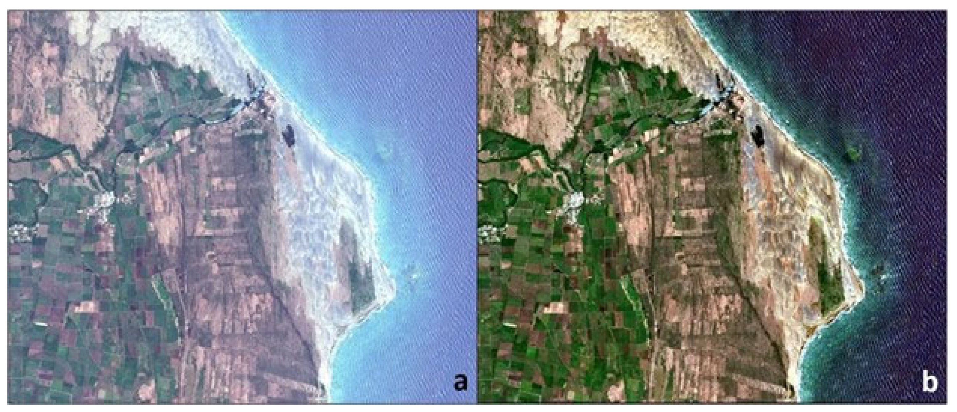
Figure 1.
Inexact synchronicity is a source of error for ancillary image application as shown in the following example: (a) 14 August 2021 Sentinel 2 TOAR RGB of southern Minnesota, (b) the cirrus band (B10) of the same scene, and (c) the cirrus band (B09) of Landsat 8 taken about 18 min before. Cirrus affects visible bands as in (a).

Figure 2.
An example 100 m resolution (10 × 10 pixel grid cell) Atm-I grayscale for the 8-22-21 S2 tile over Lake Tahoe, CA, USA. At least some ground signal must remain for correction (exceeded in portions of this image).
Figure 2.
An example 100 m resolution (10 × 10 pixel grid cell) Atm-I grayscale for the 8-22-21 S2 tile over Lake Tahoe, CA, USA. At least some ground signal must remain for correction (exceeded in portions of this image).

Figure 3.
CMAC conceptual model illustrated as a dashed line expressing the effect upon any pixel, dark to bright, from a single level of atmospheric aerosol. SR is surface reflectance. The TDL crosses the x-axis at the axis point.
Figure 3.
CMAC conceptual model illustrated as a dashed line expressing the effect upon any pixel, dark to bright, from a single level of atmospheric aerosol. SR is surface reflectance. The TDL crosses the x-axis at the axis point.


Figure 5.
Data extracted from S2 images from 2021 over an area of interest with consistent reflectance in Reno, Nevada that experienced wide swings of aerosol concentration from regional wildfire smoke. The application of such invariant locations is described further in Section 2.4 below. DN refers to reflectance scaled by 10,000.

Figure 6.
Salon de Provence, France region: a calibration target (arrows) in S2 TOAR regional images 16 June 2021 under light haze (a,d) and 8 March 2021 under moderate haze from wildfire smoke (b,e). A Google Earth image (c) of the target shows the 30 m × 30 m black and white panels.
Figure 6.
Salon de Provence, France region: a calibration target (arrows) in S2 TOAR regional images 16 June 2021 under light haze (a,d) and 8 March 2021 under moderate haze from wildfire smoke (b,e). A Google Earth image (c) of the target shows the 30 m × 30 m black and white panels.

Figure 7.
The Reno QIA outlined in red on this S2 image from 6 March 2021 is located just northeast of the Reno, NV airport. The polygon was drawn to exclude vacant lots that might harbor unmanaged vegetation.
Figure 7.
The Reno QIA outlined in red on this S2 image from 6 March 2021 is located just northeast of the Reno, NV airport. The polygon was drawn to exclude vacant lots that might harbor unmanaged vegetation.

Figure 8.
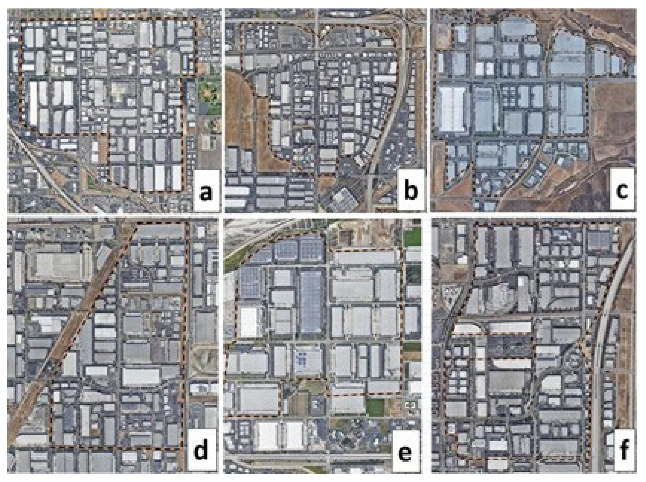
Map showing locations of six QIAs located east of Los Angeles, CA. (Source: Maxar, Earthstar Geographics and the GIS User Community). QIA locations are designated as follows: Chino (a); Ontario (b); Highgrove (c); Fontana (d); Redlands (e); and Rochester (f).
Figure 8.
Map showing locations of six QIAs located east of Los Angeles, CA. (Source: Maxar, Earthstar Geographics and the GIS User Community). QIA locations are designated as follows: Chino (a); Ontario (b); Highgrove (c); Fontana (d); Redlands (e); and Rochester (f).

Figure 9.
Google Earth closeup images of six QIAs: (a) Chino; (b) Ontario; (c) Highgrove; (d) Fontana; (e) Redlands; and (f) Rochester.
Figure 9.
Google Earth closeup images of six QIAs: (a) Chino; (b) Ontario; (c) Highgrove; (d) Fontana; (e) Redlands; and (f) Rochester.

Figure 10.
Reno QIA reflectance curves plotted for the four VNIR bands of S2 (rows). Colored curves were derived from n = 3 or n = 4 percentile averages for each band and treatment for the low-Atm-I images (clear-appearing, lacking haze). Legend values are Atm-I or average Atm-I. Curves in black are for single images that exceed Sen2Cor AC capability. Though not as accurately, CMAC corrected the extremely high Atm-I curves for the visible bands. CMAC curves are tighter (more precise) than Sen2Cor in all bands.

Figure 11.
Seven reflectance curves for the Rochester QIA by treatment (columns) and bands (rows). Each curve represents an average of four images with similar average Atm-I. Dispersion is notable for Sen2Cor in the lower limb of visible bands where high precision is needed to support applications such as precision agriculture and AI feature extraction. In CMAC, the lower limb of reflectance is comparatively precise. NIR 8A curves are virtually identical between the two methods. Rochester experienced the highest range of Atm-I levels among the SoCal QIAs.

Figure 12.
Average CV% distribution for the 22 percentile steps combined for the six QIAs; (n = 132) of CMAC and Sen2Cor. Though approached very differently, both methods show similar trends.
Figure 12.
Average CV% distribution for the 22 percentile steps combined for the six QIAs; (n = 132) of CMAC and Sen2Cor. Though approached very differently, both methods show similar trends.

Figure 13.
Percent error distribution for CMAC and Sen2Cor plotted according to the rank for the 1st through 3696th estimated error values.
Figure 13.
Percent error distribution for CMAC and Sen2Cor plotted according to the rank for the 1st through 3696th estimated error values.

Figure 14.
CMAC estimated percent error plotted together for all four VNIR bands.

Figure 15.
Percent error in Sen2Cor low surface reflectance estimates rapidly increase with Atm-I in all bands except NIR 8A. CMAC error shows a more gradual trend of increased error with increasing Atm-I level.
Figure 15.
Percent error in Sen2Cor low surface reflectance estimates rapidly increase with Atm-I in all bands except NIR 8A. CMAC error shows a more gradual trend of increased error with increasing Atm-I level.

Figure 16.
A clip from the S2 Reno image whose data are shown in Figure 10 statistics for Atm-I = 1743 and as the 22-8-2021 statistics in Supplementary Materials as “Reno QIA Curves.xlsx”. As in all other image displays in this paper, these examples are screenshots from QGIS display. (a) TOAR representation made from the full tile stretch. A full tile image stretch can be taken to visually represent the degraded TOAR mathematics of the image. The alternative, a clipped image stretch, does not appropriately represent the unbiased mathematics of the image that confronts AI and other machine analysis; such clip stretches may visibly clear some haze (but are typically accompanied by color balance problems). Color balance is a valuable indicator of potential problems that could occur through use of machine analyses. (b) CMAC clearing of the image provides the color balance conferred by the TOAR image. The features within both are darkened through hypothesized diffuse shading from aerosol particles. (c) Sen2Cor correction of the same clip displaying color balance problems and residual haze.

Figure 17.
S2 image, 5 March 2021 closeup of the Mexican Gulf Coast north of Veracruz: (a) TOAR with smoke effects from fields burned before planting; (b) CMAC v1.1 corrected.
Figure 17.
S2 image, 5 March 2021 closeup of the Mexican Gulf Coast north of Veracruz: (a) TOAR with smoke effects from fields burned before planting; (b) CMAC v1.1 corrected.

Figure 18.
L8 full tile of the Mexican Gulf Coast from 5 December 2021: (a) TOAR, (b) Atm-I, (c) LaSRC correction and (d) CMAC correction. The images were rotated from their collection angle to fit squarely.
Figure 18.
L8 full tile of the Mexican Gulf Coast from 5 December 2021: (a) TOAR, (b) Atm-I, (c) LaSRC correction and (d) CMAC correction. The images were rotated from their collection angle to fit squarely.

Figure 19.
TOAR (a) and CMAC (b) views of 8-18-2021 Planet Labs Dove satellite image over Fargo, North Dakota (20210818_175123_23_105a_3B_AnalyticMS_clip.tif cohort PS2.SD).
Figure 19.
TOAR (a) and CMAC (b) views of 8-18-2021 Planet Labs Dove satellite image over Fargo, North Dakota (20210818_175123_23_105a_3B_AnalyticMS_clip.tif cohort PS2.SD).

Disclaimer/Publisher’s Note: The statements, opinions and data contained in all publications are solely those of the individual author(s) and contributor(s) and not of MDPI and/or the editor(s). MDPI and/or the editor(s) disclaim responsibility for any injury to people or property resulting from any ideas, methods, instructions or products referred to in the content. |
© 2023 by the authors. Licensee MDPI, Basel, Switzerland. This article is an open access article distributed under the terms and conditions of the Creative Commons Attribution (CC BY) license (https://creativecommons.org/licenses/by/4.0/).
Share and Cite
MDPI and ACS Style
Groeneveld, D.P.; Ruggles, T.A.; Gao, B.-C. Closed-Form Method for Atmospheric Correction (CMAC) of Smallsat Data Using Scene Statistics. Appl. Sci. 2023, 13, 6352. https://0-doi-org.brum.beds.ac.uk/10.3390/app13106352
AMA Style
Groeneveld DP, Ruggles TA, Gao B-C. Closed-Form Method for Atmospheric Correction (CMAC) of Smallsat Data Using Scene Statistics. Applied Sciences. 2023; 13(10):6352. https://0-doi-org.brum.beds.ac.uk/10.3390/app13106352
Chicago/Turabian StyleGroeneveld, David P., Timothy A. Ruggles, and Bo-Cai Gao. 2023. "Closed-Form Method for Atmospheric Correction (CMAC) of Smallsat Data Using Scene Statistics" Applied Sciences 13, no. 10: 6352. https://0-doi-org.brum.beds.ac.uk/10.3390/app13106352
Note that from the first issue of 2016, this journal uses article numbers instead of page numbers. See further details here.