A Metaheuristic Harris Hawks Optimization Algorithm for Weed Detection Using Drone Images

Abstract

There are several major threats to crop production. As herbicide use has become overly reliant on weed control, herbicide-resistant weeds have evolved and pose an increasing threat to the environment, food safety, and human health. Convolutional neural networks (CNNs) have demonstrated exceptional results in the analysis of images for the identification of weeds from crop images that are captured by drones. Manually designing such neural architectures is, however, an error-prone and time-consuming process. Natural-inspired optimization algorithms have been widely used to design and optimize neural networks, since they can perform a blackbox optimization process without explicitly formulating mathematical formulations or providing gradient information to develop appropriate representations and search paradigms for solutions. Harris Hawk Optimization algorithms (HHO) have been developed in recent years to identify optimal or near-optimal solutions to difficult problems automatically, thus overcoming the limitations of human judgment. A new automated architecture based on DenseNet-121 and DenseNet-201 models is presented in this study, which is called “DenseHHO”. A novel CNN architecture design is devised to classify weed images captured by sprayer drones using the Harris Hawk Optimization algorithm (HHO) by selecting the most appropriate parameters. Based on the results of this study, the proposed method is capable of detecting weeds in unstructured field environments with an average accuracy of 98.44% using DenseNet-121 and 97.91% using DenseNet-201, the highest accuracy among optimization-based weed-detection strategies.

1. Introduction

Precision agriculture and measures have improved production, quality, and working conditions by reducing manual labor. These things help make farming sustainable. Modern farmers use digitally controlled farm plants and unmanned aerial vehicles (UAVs) for monitoring and forecasting. Affordable drones can image ground data with geolocations. This helps users understand ground information better. Multispectral and RGB drones can image the near-infrared section of the electromagnetic spectrum above crops, revealing their health [1]. Satellites, aerial photography, unmanned aerial vehicles (UAVs), geographic information systems (GIS), global positioning systems (GPS), variable rate application (VRA), and geostatistics are all examples of remote sensing utilized in precision agriculture. This method of geostatistics is a branch of applied statistics that is closely linked to precision farming. Through data transformation, it is possible to discover the values of the attributes at unsampled points on the field by calculating their spatial dependency and spatial structure. Interpolation is a common technique for estimating values at nearby points when exact values are unavailable. Variography is a type of geographical modeling utilized in precision agriculture, while kriging is the term used to describe spatial interpolation [2].

Precision farming has numerous significant applications in arable land, one of which is enhancing the efficiency of fertilizer utilization based on the three macronutrients, namely nitrogen, phosphorus, and potassium. In conventional agricultural practices, fertilizers are typically applied uniformly across the entire field at predetermined intervals throughout the year. Precision farming enables the optimization of agricultural practices by increasing applications in certain locations and decreasing applications in others. Numerous environmental hazards are commonly attributed to the escalating usage of agricultural inputs, resulting in the leaching of nitrogen and phosphorus from fields into both surface and groundwater sources. The utilization of PF technology enables the precise application of fertilizers in varying spatial and temporal dimensions, therefore enhancing the efficacy of variable rate application [1,3]. Weeds are a major threat to crops because of their detrimental effects on neighboring plants and their ability to stunt plant growth and reduce nutrient intake. If weeds are not controlled quickly and efficiently, they can diminish agricultural output by 20–80% [4].

Weeds compete with crops for limited resources, making them a problem in agricultural settings. Their strong competition with agricultural plants for nutrients, water, sunlight, air, etc. affects production and yield, which have monetary value. Weeds reduce output by 34% worldwide [4]. Wheat yields drop 48–60% [5] and sesame yields drop 50–75%. Weeds degrade crop output and quality. Farmers spend billions of dollars yearly on weed management in an attempt to achieve satisfactory weed control and higher crop productivity. Reduced yields and worse quality products are the direct results of ineffective weed management in horticulture crops [6]. The use of chemical and cultural control strategies may have unintended consequences for the environment. Low-cost technology for early weed identification and mapping will make weed management more effective and sustainable. Using early weed management can cut down on agricultural diseases and pests and boost crop yields by as much as 34% [7]. Many strategies exist for weed control, and each one is eco-friendly in some way. One of the most promising of these techniques is image processing. Image processing makes use of UAVs (unmanned aerial vehicles) to survey fields for weeds and other unwanted plants. UAVs are useful in agriculture because of their speed and efficiency in covering large areas, without damaging the soil or compacting it [8]. Converting UAV data into actionable intelligence remains a significant hurdle. Conventional data gathering and classification cannot be automated because of the human labor necessary for segment size adjusting, feature selection, and rule-based classifier development.

The primary focus of agricultural mechanization research is on improving crop yields while reducing weed infestations. Data scientists have found weed detection to be a fruitful field of study due to the prevalence of algorithms based on machine learning [9]. To classify agricultural and weed plants, many researchers have turned to computer vision techniques [10]. Significant advances have also been made through the publication of several deep-learning and hand-crafted models [11] As a subfield of both ML and AI, deep learning (DL) is making significant progress toward automating precision agriculture [12,13]. DL has made important contributions to many fields of agriculture [14,15], including: disease detection [16], crop plant detection and counting [17], crop row detection [18], crop stress detection [19], fruit detection and freshness grading [20], fruit harvesting [18,21], and site-specific weed control [21].

Hand-crafted methodologies require substantial testing to extract essential features and may also be insufficiently robust in complicated environments and biological variability [20]. CNNs have improved object detection [22]. CNNs can be taught end to end without feature extraction, making them superior at classifying and detecting weeds [21].

This paper’s contribution can be summarized as follows:

• A deep-learning-based framework, “DenseHHO”, that is designed to improve the detection of weeds using pre-trained CNNs such as DenseNet-121 and DenseNet-201 is presented.
• The devised model’s CNN architecture is adopted based on the analysis of weed images captured by sprayer drones structured as an optimization problem addressed by an HHO natural-inspired algorithm.
• The performance of the devised model is improved using HHO for binary class classification to automatically select as well as optimize the CNN’s hyperparameters.
• The performance of DenseHHO has been evaluated through a comparative analysis and performance evaluation based on various performance metrics.

This paper is organized into five sections. The problem addressed in this paper is introduced in Section 1, along with a summary of the proposed solution. Section 2 discusses the major milestones in the weed-detection literature. Section 3 describes the materials and procedures used in the proposed solution. Section 4 explains the proposed algorithms and solutions, while Section 5 discusses the experimental results. Section 6 concludes with a discussion of the findings.

2. Related Work

Traditional machine-learning approaches require a limited sample size, a quick training period, and a few graphics-processing units to calculate picture texture, shape, hue, or spectral properties to identify crops or weeds.

There have been several attempts in the literature to generate weed maps from unmanned aerial vehicle (UAV) images using a variety of classification approaches [23,24]. However, recent state-of-art work shows [25] that machine-learning algorithms, when dealing with complex data, are more accurate than conventional algorithms. The utilization of high-resolution UAV imagery and the application of the random forest (RF) algorithm for agricultural mapping have been demonstrated to yield advantageous outcomes [7,8,26]. SVM classifier is also commonly used for the classification of crops and weeds [27,28].

For early cranesbill seedling extraction [29], improved Mask RCNN was used. The proposed method separated weeds from the original image, allowing an increase in yield.

Deep neural networks (DNNs) were used to segregate weed crops [30]. Four additional elements improved segmentation accuracy, improving weed detection for complicated shapes in tough environments without image preprocessing or data conversion. Recognition accuracy is higher than the machine-learning techniques that use manually specified features. Deep learning was used to detect ryegrass species from weeds in [31]. The dataset included photos of ryegrass seedlings, maculata, hederacea, and officinale weeds—16,116 weed-free samples and 18,230 weedy samples. The dataset was trained with GoogLeNet, AlexNet, and VGGNet. VGGNet’s F-score was the highest. Maculata, hederacea, and officinale had success rates of 92.65%, 99.84%, and 97.37%, respectively.

Convolutional Neural Network (CNN) architectures are better at classifying plant species. The AlexNet model had a 99.5% accuracy on a grass-broadleaf dataset, according to [32]. In categorizing four weed species, Ahmad et al. [33] attained an average accuracy of 98.90% for VGG16, 97.80% for ResNet50, and 96.70% for Inceptionv3.

Beeharry and Bassoo [34] tested ANN and AlexNet weed recognition algorithms on UAV photos. AlexNet’s weed-detection rate was over 99%, while the ANN’s was 48% on the same dataset.

Metaheuristic optimization rarely optimizes weed categorization models. Computer vision is used in [35] to recognize potato plants and three weed categories. The proposed method improves NN-classifier performance using two metaheuristic methods, the cultural algorithm by which the five most significant features are selected and the harmony search method for finding the network architecture. The system’s identification accuracy was 98.38%.

ANN was used to categorize narrowleaf and broadleaf weed species and rice species in [36]. A total of 97 rice images, 77 narrowleaf, and 52 broadleaf images were used. Particle swarm optimization (PSO) and the bee algorithm (BA) identified efficient features. The ANN-BA method was the best. The study found an arithmetic mean accuracy of 92.02% and geometric mean accuracy of 90.7%.

A unique optimization strategy to improve weed image-classification accuracy was given by the authors in [37], which categorizes spraying drone weed and wheat shots differently. SVM, NN, and KNN were the classifiers optimized using cosine, sine, and gray wolf optimizers. The optimized voting classifier showed 97.70% detection accuracy, 98.60% F-score, 95.20% specificity, and 98.40% sensitivity.

The authors in Ref. [38] introduce a technique called Modified Barnacles Mating Optimization with Deep-Learning-based Weed Detection (MBMODL-WD). MBMODL-WD uses Gabor filtering (GF) for noise removal, DenseNet-121 for feature extraction, and the MBMO algorithm for hyperparameter optimization. Elman Neural Network (ENN) was used to classify weeds. MBMODL-WD performed with maximum accuracy of 98.99%.

3. Proposed Framework

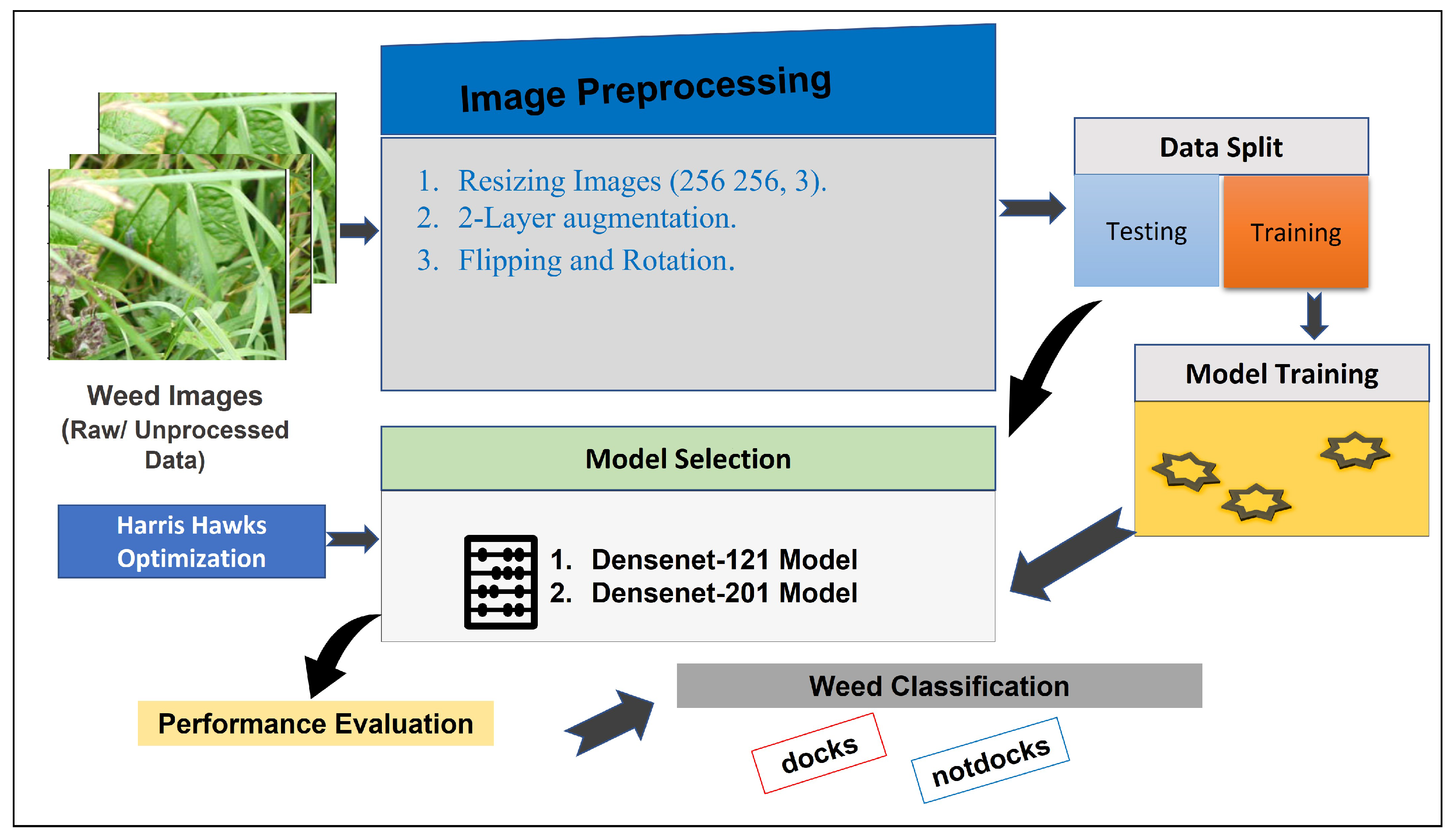
Detailed descriptions of the proposed method are provided in this section. Furthermore, the dataset used is described in detail. The proposed approach involves loading weed data directly into the DenseHHO deep modeling framework for the purpose of arriving at a final decision. Figure 1 depicts a block diagram of the designed DenseHHO framework from beginning to end. The first step in the analysis process was to collect and prepare the dataset. The next step involves separating the data into two groups: training and testing. Data preparation techniques are implemented in training sets first, then applied to test sets to avoid data leakage and overload. To classify weed data, two models were developed, namely DenseNet-121 and Densenet-201. Then, the best-performing features from each model were used for the classification. A natural-inspired evolutionary algorithm was used for DenseHHOś DNN networks to automatically optimize the network’s hyperparameters based on their accuracy. A final step involves testing and evaluating the performance of the models developed.

3.1. Dataset Collection and Preprocessing

A detailed description of the dataset of this study and the key pre-trained models is provided in this section. UAVs equipped with cameras are capable of capturing field crops using sensors. An autonomous aerial sprayer drone was used to capture the images of wheat crops in this study, and the dataset is freely available on Kaggle (https://www.kaggle.com/datasets/gavinarmstrong/open-sprayer-images, accessed on 4 February 2023). The “Open Sprayer Images” dataset includes images related to agricultural sprayers. The UAV type typically used in conjunction with sprayers is a multirotor UAV or a fixed-wing UAV. The “Open Sprayer Images” dataset provides sample images and visual representations associated with the dataset. However, the creator did not add any details about the UAV or Flight parameters. Furthermore, it is explained that all the collected photos should be retaken from a higher elevation. Based on the assumption that the sprayer will cover a 3 m width, he might be able to use one camera mounted high enough to view 3.5 m with 0.5 m of overlap. The resolution and size of the photos can be easily changed by changing the camera settings or dividing the photos into sections before processing. Dock leaves do stand out quite well from the grass background, so hopefully, a picture taken from a greater distance will provide enough information to classify the leaves. Images of broad-leafed docks and pictures of shorelines without broad-leafed docks are included in the dataset. In the context of weed detection, “dock” typically refers to a group of weed species belonging to the Rumex genus. Common dock species include broadleaf weeds such as curly dock (Rumex crispus) and broadleaf dock (Rumex obtusifolius) [19]. These plants typically have broad leaves with distinctive veining and are often considered undesirable in agricultural or landscaping settings. Figure 2 and Figure 3 show examples of images from this dataset. The dataset is comprised of 1176 wheat and 4851 weed images, respectively. A total of 540 images of weeds and 130 images of wheat are included in the testing set.

As the images were derived from various sources, there may be variations in shapes, brightness, and contrast. All Weed-Spray images were resized to (256, 256, 3), and augmented using a 2-layer augmentation. To increase the diversity of the gathered datasets and making our models more robust, all fused weed scans have undergone a two-layer augmentation process:

• Random Flip: This layer will perform horizontal and vertical mirroring through the reversal of rows/columns of pixels.
  $tf.keras.layers.RandomFlip(mode=‘horizontal\_and\_vertical’)$.
• Random Rotation: This layer will apply random rotations to each image. The factor here is a float represented as a fraction of 0.1.

3.2. Pre-Trained Models

CNN is a subset of the multilayer neural network, which analyzes the pixels in images to extract information. Huang et al. proposed DenseNet-102 and DenseNet-201 [39] as a deep CNN architecture in their paper “Densely Connected Convolutional Networks”. DenseNet creates dense networks by connecting every layer to every other layer in a feed-forward manner. All subsequent layers receive their feature maps from each preceding layer as an input, and all subsequent layers receive their feature maps as output. DenseNet-102 and DenseNet-201 have demonstrated state-of-the-art performance on several benchmark image-classification datasets with significantly fewer parameters than other top-performing pre-trained models, such as Inception-v4 and ResNet-152. DenseNet-121 and DenseNet-201 are employed in the devised models, which have proved to be exceptionally effective in classifying images. Additionally, using such a CNN-based pre-trained model, an automated mechanism for feature extraction has been implemented in the current work. The structures used for DenseNet-121 and DenseNet-201 consist of five layers. The layers are the input layer, the model layer (either 121 or 201), the flatten layer, and the dense layer, which contains 128 cells and an activation function. There are two cells and an activation equation in the dense layer, which is the output layer. As a result, this structure is the general structure used because no changes have been made to the basic structure of any model, but the only difference between the two structures is the model layer, which has been replaced by the specific model version. This approach resulted in the creation of a fixed feature extractor, in which the output layer was removed, and the entire network was utilized. For the devised models, the feature map is represented based on the following equation:

$$y_{(i,j,k)}=\sigma \left(\sum _{u=1}^U\sum _{v=1}^V\sum _{c=1}^C{W}_{(u,v,c,k)}{X}_{\left(\right(i+u-1),(j+v-1,c\left)\right)}\right)$$

(1)

where activation values $y_{(i,j,k)}$ represent the activation value in the kth feature map, activation function $\sigma$ represents the activation function, and input value $X_{(i,j,c)}$ refers to the input channel value of $(i,j)$, $W_{(u,v,c,k)}$ refers to the weight value for the kth feature map at position $(u,v)$ of the cth input channel and U, V, and C, respectively, represent the filter’s width, height, and channel count. This is followed by the calculation of output using the following equation:

$$y_{\left(k\right)}=\sigma (\sum _{j=1}^J{W}_{j,k}{X}_j+b_k)$$

(2)

3.2.1. DenseNet-121 Model

DenseNet-121 is a member of the DenseNet family consisting of 121 layers of Convolutional layers (117-Convolutional, 3-transition, and 1-classification) with four dense blocks separated by transition layers. Convolutional layers are interspersed between the dense blocks, forming convolutional layers. Every block is composed of a 1 × 1 convolutional layer followed by a 3 × 3 convolutional layer. Concatenating the outputs of each dense block with those of the previous dense block is performed using a transition layer. An average pooling layer of 2 × 2 is used to downsample the feature maps after a convolutional layer of 1 × 1 reduces the number of channels. The devised model setting is shown in

Table 1. The DenseNet-121 Model Structure.

Layer (Type)	Output Shape	Param #
Input_2 (InputLayer)	[(None, 256, 256, 3)]	0
sequential (Sequential)	[(None, 256, 256, 3)]	0
densenet121 (Functional)	(None, 8, 8, 1024)	7,037,504
flatten (Flatten)	(None, 65, 536)	0
dense (Dense)	(None, 128)	8,388,736
Dense_1 (Dense)	(None, 2)	258
Total Params: 15,426,498
Trainable Params: 15,342,850
Non-trainable Params: 83,648

.

3.2.2. DenseNet-201 Model

This model, as shown in

Table 2. The DenseNet-201 Model Structure.

Layer (Type)	Output Shape	Param #
Input_2 (InputLayer)	[(None, 256, 256, 3)]	0
sequential (Sequential)	[(None, 256, 256, 3)]	0
densenet121 (Functional)	(None, 8, 8, 1024)	18,321,984
flatten (Flatten)	(None, 65,536)	0
dense (Dense)	(None, 128)	15,728,768
Dense_1 (Dense)	(None, 2)	258
Total params: 34,051,010
Trainable params: 33,821,954
Non-trainable params: 229,056

, has more layers and is more complex than DenseNet-121. There are 201 layers, divided into four dense blocks, each preceded by a transition layer. Every dense block has multiple convolutional layers with fully connected layers between them. An input fully connected layer is made up of a 1 × 1 convolutional layer, which is used to reduce the number of input channels, followed by a 3 × 3 convolutional layer to transform it non-linearly. After each dense block, the output is concatenated with the output of the previous dense block. To downsample the feature maps, the transition layer uses a 1 × 1 convolutional layer, followed by a 2 × 2 average pooling layer.

3.3. Harris Hawks Optimization Algorithm

Data-driven AI models are represented by three major components: the data they use, the parameters used to train them, and the architecture of the networks they use. To perform tasks with maximum efficiency, any deep-learning model must achieve a proper balance among these elements. To confirm the design of the model, a set of initial parameters is used in several trials, and the performance of the model is measured within each trial. Additionally, there are optimization concerns associated with increasing network depth. Furthermore, incorrect selection of hyperparameters may result in suboptimal results. The hyperparameter tuning and result analysis for DenseHHO can be a time-consuming process. Consequently, the process of hyperparameter optimization must be performed to iteratively search for the most optimal values based on the training data and update them accordingly. The Harris Hawk Optimization algorithm (HHO) [40,41] is a metaheuristic optimization method used for the DenseHHO framework. HHO was inspired by Harris hawks’ hunting behavior. The HHO algorithm can solve various optimization problems, including function optimization, feature selection, and parameter optimization for machine-learning models. To implement the algorithm, the following steps must be taken. A significant difference between HHO and other optimization algorithms lies in the introduction of the concepts of elite and non-elite hawks instead of following a strict hierarchical structure. As a result, elite hawks take the lead in the search process, representing the fittest solutions. To maintain their position, they mimic the behavior of the best hawks in the population. In this manner, the algorithm can converge toward promising solutions using this exploitation mechanism. Three types of hunting behavior are observed in Harris hawks:

• Exploration: Hawks fly randomly to discover new areas in which they can search.
• Exploitation: Hawks attempt to improve upon the solutions provided by the most successful individuals.
• Intensification: Hawks coordinate their efforts to search for prey.

Algorithm 1 provides the detailed steps of the proposed DenseHHO framework. After initializing the pre-trained model, the HHO will be used to optimize the network hyperparameters. To search for an optimal solution, the HHO uses the following hunting behavior:

$$X_i^{t+1}=X_i^t+rand\left(\right).(X_j^t-X_k^t),$$

(3)

where $rand\left(\right)$ is a random number between 0 and 1, j and k are two randomly chosen hawks, and t is the current iteration. The hawks guide the optimization process by updating their positions in accordance with those of other hawks using the following:

$$X_i^{t+1}=\frac{\left(X_i^t\right)+\left(X_j^t\right)}{2}+rand\left(\right).(X_j^t-X_k^t),$$

(4)

Algorithm 1 The suggested DenseHHO framework pseudocode

Input:Weed Images Dataset Dt, CNN- Hyperparameters, Objective Function F Output:best model architecture, Performance Metrics. 1: Create TestDataset, and trainDataset; 2: Set Dimension d, optimization iteration $T_{\left[max\right]}$, and objective function $Accuracy$ 3: for trainDataset portion Tt do 4:     Train TLD using DenseNet-121 and DenseNet-201. 5:     Initialize a population P of n hawks with random positions $X_i$, where $i=1,2,\cdots ,n$. 6:     Create solution $S{L}_0$← InitialPopulationGeneration. 7:     Set t← 0 an initial optimization step, Counter C← 1,DimensionList DL[ ]. ▹ Use HHO to learn the Densenet model hyperparameters for $T_{max}$ optimization iteration 8:     Use ImageNet to initialize each pre-trained network. 9: while ($t\le T_{max}$) do 10:     while ($C\ne N_{max})$ do 11:         Create an initial solution list ML[C]. 12:         Sort the hawks in descending order of fitness value. 13:         Choose the top $p\%$ of the hawks and update the positions and velocities of each hawk in accordance with its hunting behavior using the following Equation (3) 14:         Determine which hawks will form the next generation based on their performance by choosing the remaining $(1-p)$ of the hawks and updating their positions using the following Equation (4). 15:         calculate fitness Function (TLD, DL, Tl, Ts, V). 16:         Use Equation (4) to select the best solution HL. 17:         if (HL outperforms ML) then 18:            Update the Harris values( Equation (3)). 19:            $ML\leftarrow HL$. 20:         Apply same TLD, ML, TL, Ts, VR 21:         if ( There is no more space in the archive) then 22:            Allow new Harris solution to be added by deleting some iterations. 23:         Update Solutions Using Harris(HL, DL) 24:         i++. 25:         t++. 26:         Apply HHO Optimizer for Training Options (F, H1, H2, H3, H4, H5) ▹ The best overall score and solution using optimizer range 27:         Train DL using bestscore 28:         Fuse Weed images’ features of DLs 29:         Calculate performance metrics for BM based on Training Data; 30:         Classify the fused Weeds features. 31:         Return: BM, performance evaluation metrics.

3.4. Experimental Setting

Our optimization algorithm uses the Adam optimizer at a learning rate of 0.001, a batch size of 32, and a training schedule of 50 epochs. A list of loss functions is created after each epoch using the categorical cross-entropy loss function.

The number of epochs used for training is five, with 188 iterations per epoch. The optimizer used for DenseNet-121 and DenseNet-201 is “Adam” with $learning\_rate$ = 0.0001 and $loss=categorical\_crossentropy$. In addition, the learning _rate_reduction was used with these settings: $monitor{=}^{\prime }val\_accurac{y}^{\prime }$, $patience=2$, $verbose=1$, $factor=0.5$, $min\_lr=0.00001$. HHO algorithm settings are shown in

Table 3. HHO Parameter Setting.

Parameter	Purpose	Value
Fitness_function	A user-defined function that takes a set of hyperparameters as input and returns a fitness value that represents the performance of a machine-learning model trained with those hyperparameters.	The maximum validation accuracy and minimum validation loss
objf	The objective function to be optimized.	Accuracy
lb	A numpy array representing the lower bounds of the search space.	0
ub	A numpy array representing the upper bounds of the search space.	1
dim	The number of dimensions in the search space.	10
SearchAgents_no	The number of search agents (i.e., hawks) to be used in the optimization algorithm.	30
Max_iter	The maximum number of iterations to run the optimization algorithm.	2

.

3.5. Performance Parameters and Evaluation Metrics

Several measures were used to evaluate the proposed DenseHHO, including accuracy, F1_score, Sensitivity, and Specificity. According to the ratio between the number of Dock samples correctly classified to the total number of samples, the [accuracy] value is calculated. This evaluation metric can be calculated using Equations (5)–(8), where [True Positive TP] represents the number of Dock, and Not-Dock images that have been correctly classified; [True Negative TN] represents the number of weed images that have been misclassified. Additionally, macro average scores can be used to evaluate the overall performance of the model across several sets of data. This study uses the macro average to measure the performance of the different classes. The macro average F1-score is calculated by first computing the accuracy and recall of each class label from n classes, followed by calculating the unweighted arithmetic mean and weighted average score as shown in Equations (9)–(12). The DenseHHO is evaluated with confusion matrices (CMs). A classification method’s CM represents the characteristics of that method’s classification performance during its execution.

$$Accuracy=\frac{(TP+TN)}{(TP+FP+FN+TN)}$$

(5)

$$Sensitivity\left(Recall\right)=\frac{TP}{(TP+FN)}$$

(6)

$$Specificity\left(Precision\right)=\frac{TP}{(TP+FP)}$$

(7)

$$F1\_score=\frac{TP}{(TP+0.5(FP+FN\left)\right)}$$

(8)

$$Macroavgprecision\left(MAP\right)=\frac{{\sum }_{i=1}^{n}TP}{n}$$

(9)

$$Macroavgrecall\left(MAR\right)=\frac{{\sum }_{i=1}^{n}FN}{n}$$

(10)

$$Macroaverage=\frac{2(MAP\times MAR)}{(MAP+MAR)}$$

(11)

$$Weightedaverage=\frac{(1+\beta )\times (Precision\times Recall)}{(Recall+({\beta }^2\times Precision)))}$$

(12)

where $0<\beta <1$ add weight to the $Precision$, and $\beta$ >1 add weight to the $Recall$.

4. Results

The purpose of our study was to evaluate the accuracy of two pre-trained deep-learning models for the classification of weed images. in the following subsections, we will detail the experimental setting and the obtained results.

4.1. Model Evaluation Performance

The experimental dataset consisted of 6697 images of weeds that were grouped into two categories. Using a 70-30 split, the dataset was divided into training and testing sets. Five-fold cross-validation was used to train and evaluate the models. A total of 6027 images were used to train the model and 670 images were used to test its accuracy. In

Table 4. DenseHHO Classification Accuracy.

Model	Accuracy	F1_Score	Sensitivity	Specificity
DenseNet-121	98.44%	97.61%	99.10%	97.30%
DenseNet-201	97.91%	97.91%	97.50%	98.00%

, we provide the obtained accuracy for each model as well as other evaluation metrics. The training and validation confusion matrix for model 1 and model 2 is given in Figure 4, Figure 5, Figure 6 and Figure 7.

An imbalance between classes in the dataset is not taken into account when calculating the classification accuracy alone, which can result in misleading results when the dataset has a skewed distribution of classes. It is, therefore, important to take into account the imbalance between classes in the dataset by evaluating the “weighted accuracy” and “macro accuracy” assessment. For DenseNet-121 and DenseNet-201,

Table 5. The testing performance of HHO-optimized DenseNet-121.

	Precision	Recall	F1_Score	Support
0	0.95	0.91	0.93	130
1	0.98	0.99	0.98	540
accuracy			0.97	670
macro avg	0.96	0.95	0.96	670
weighted avg	0.97	0.97	0.97	670

and

Table 6. The testing performance of HHO-optimized DenseNet-201.

	Precision	Recall	F1_Score	Support
0	0.98	0.92	0.94	130
1	0.98	0.99	0.99	540
accuracy			0.98	670
macro avg	0.98	0.95	0.97	670
weighted avg	0.98	0.98	0.98	670

provide the evaluation report for each model considering their macro and weight average.

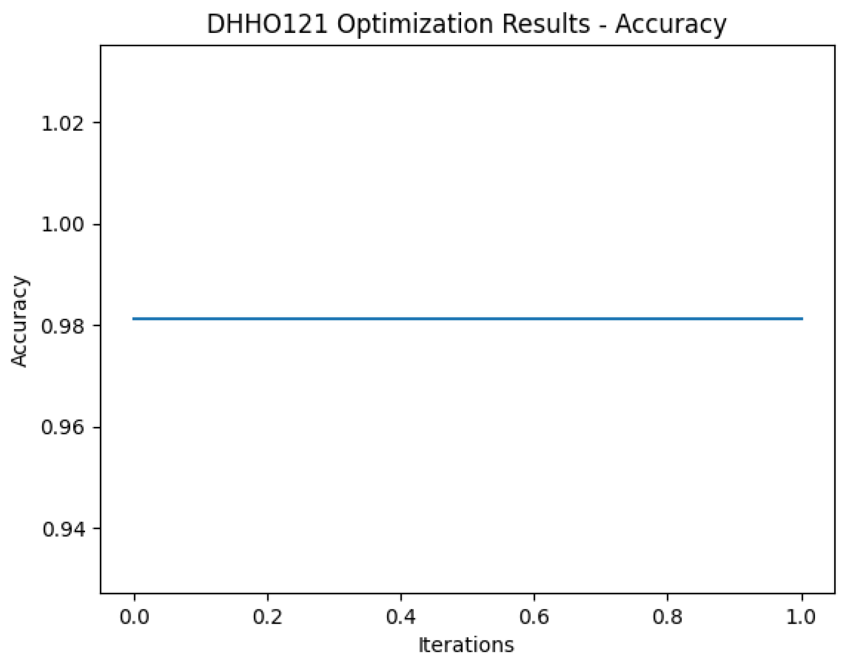
The convergence of an optimization algorithm is typically determined by comparing the difference between two consecutive iterations of the objective function. The algorithm is said to have converged if the difference falls below a certain threshold. If further iterations of the algorithm do not produce a significant improvement in the objective function, the optimization algorithm has converged. The maximum validation accuracy and minimum validation loss are then derived as an objective function for the fitness solution, and convergence criteria are established that the algorithm will terminate once the gradient norm does not exceed 1.0. The HHO coverages for 5 epochs with 188 iterations per epoch, which is shown in Figure 8 and Figure 9 for the devised framework considering DenseNet-121 and DenseNet-201, respectively. After several iterations of the algorithm, we obtain a solution of x = 0.98. As a result of this convergence, the algorithm has reached a solution that is very close to its optimal value. The best solution obtained by HHO is a 10-dimensional vector whose values are:

$$\left[\begin{array}{ccccc}0.41220429& 0.51325094& 0.14969204& 0.26833381& 0.60773674\\ 0.84484728& 0.98244724& 0.98372854& 0.06231934& 0.14492935\end{array}\right]$$

and for DenseNet-201, based on the HHO algorithm, the best solution is:

$$\left[\begin{array}{ccccc}0.88840973& 0.82984462& 0.17273697& 0.42786396& 0.93121754\\ 0.90590804& 0.6815667& 0.83325338& 0.10811796& 0.86986838\end{array}\right]$$

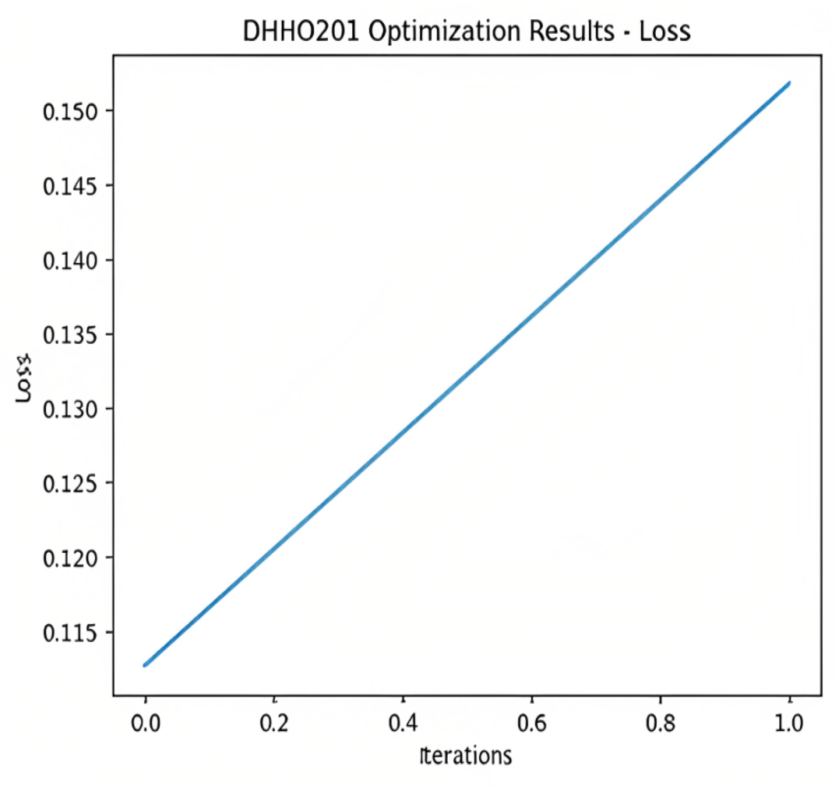
Figure 10 and Figure 11 plot the training progress of DenseHHO. Additionally, Figure 12 and Figure 13 plot the testing progress of DenseHHO. The initial test accuracy is higher than the training accuracy for the first few iterations, but as the training epoch proceeds, the test and training accuracy become more similar. The training and test efficiencies were close to 98% after the second iteration of training. Training and test accuracy increased as the iteration progressed. The best accuracy value of the objective function found by HHO for the first and second models: 98.44%, and 97.97% consequently.

4.2. DenseHHO Performance Compared to State-of-the Art

This section presents a comparison and evaluation of DenseHHO efficiency with state-of-the-art algorithms. An analysis of the proposed algorithm compared with that of peer competitors is provided in

Table 7. Performance comparison of DenseHHO and state-of-the-art-related works—Neural networks (NNs), Support vector machines (SVMs), and K-nearest neighbors (KNN).

Ref.	Target Images	Methodology	Performance	Optimization
[31]	Ryegrass species & three distinct weed types	VGGNet	F-Score: maculate-92.65%, hederacea-99.84%, officinale-97.37%	No
[32]	Plant species	AlexNet	Accuracy-99.5%
[33]	Four weed species.	VGG16, ResNet50, Inceptionv3	Accuracy VGG16-98.90%, ResNet50-97.80%, Inceptionv3-96.70%,	No
[34]	Weed	AlexNet ANN	Accuracy AlexNet-99%, ANN-48%.	No
[36]	Rice plant species & weeds	ANN Bee Algorithm (BA)	Accuracy-92.02%	Yes
[37]	Weed & wheat	NNs, SVMs,& KNN & hybrid of sine cosine & gray wolf optimization.	Accuracy-97.70%	Yes
[38]	Weed	DenseNet-121 MBMO	Accuracy-98.99%.	No
DenseHHO	Weed & wheat	DenseNet-121 & DenseNet-201 optimized with HHO	Accuracy: DenseNet-121-98.44% DenseNet-201-97.61%	Yes

. There are three columns in this table corresponding to types of purpose, namely methodology, classification accuracy, and the use of optimization algorithm. A comparison of the classification accuracy is taken from published papers and compared with the implementation of DenseHHO. From Table 4, there is a consistent performance level across the two classifiers of the network. The findings of the study demonstrate that DenseHHO yielded extremely consistent and high levels of accuracy with the same computational complexity and storage as the existing technique.

5. Discussion

Detecting undesirable plants, or weeds, plays a significant role across a variety of sectors and has significant implications for society as a whole. It is possible to increase agricultural productivity, protect natural ecosystems, and improve the quality of our environment by effectively identifying and controlling weeds. Plants cultivated in soil compete with weeds for resources such as water, nutrients, and sunlight. In addition to hindering crop growth, they can decrease yields and result in economic losses for farmers. To mitigate these negative effects on agriculture, early detection, and effective weed-management strategies are essential. Using artificial intelligence and machine learning, weed-detection systems can be improved in accuracy and efficiency, allowing them to identify weed species with greater accuracy and reliability. A more effective and sustainable management practice can be achieved across the agricultural and environmental sectors using this information to help researchers, farmers, and land managers make informed decisions about weed-control strategies. The current study examines the effects of the HHO algorithm to boost weed classification accuracy using two different CNN-based pre-trained models. Optimization algorithms can be used to tune hyperparameters in pre-trained models to improve their performance on specific tasks. Hyperparameters are parameters that are set before training begins and cannot be learned from the data. Examples of hyperparameters include the learning rate, the number of layers in the network, and the size of each layer. A significant achievement of the HHO algorithm is that it was able to find a set of hyperparameter values that resulted in the best accuracy value for weed classification.

An objective function’s accuracy value indicates the performance of the deep-learning model with the corresponding hyperparameters. HHO found the best accuracy value of 98.44% and 97.97% (as shown in Figure 4 and Figure 5), which is close to 100%. The results indicate that the deep-learning model with the best set of hyperparameters is capable of accurately classifying the weed collected data. This level of accuracy is quite high and indicates that the model has the potential to be useful in a wide range of real-world applications. As part of testing the generalization ability of the devised methodology over imbalanced complex datasets, DenseNet-121 and DenseNet-201, Figure 5 and Figrue 6 provide training accuracy assessments for both macro and weighted accuracy. A 100% weighted accuracy means that the model correctly classified all instances in the dataset, regardless of their class, and that the model was able to handle any class imbalance in the dataset. It is crucial to determine the convergence of an optimization algorithm to determine how quickly it can find a solution. Slow-converging algorithms may require many iterations to find a sufficiently good solution, whereas fast-converging algorithms may find a good solution in fewer iterations. The concept of convergence in optimization refers to the point at which an algorithm stops searching for a better solution and settles on a solution that is considered sufficiently good. After several iterations of the algorithm, we obtain a solution of x = 0.98 for five epochs with 188 iterations per epoch as shown in Figure 8 and Figure 9. At this point, the gradient at the current solution is small, indicating that the objective function is nearly flat. It can be concluded from this result that the algorithm has found a solution that is very close to the optimal solution and that further iterations are not necessary. The DenseNet-121 shows a 99.96% training accuracy (Figure 4), which indicates that it can learn training data correctly; however, a test accuracy of 97.8% indicates that it is also able to generalize well to unknown data with an average loss of 0.125 (Figure 12). The results shown in Figure 13 indicate that DenseNet-201 accurately predicted weed cases based on an average loss of 0.135. HHO is a relatively new method of solving optimization problems compared to other optimization algorithms such as GA and PSO. Despite this, there are several limitations to the HHO algorithm, such as the performance of the algorithm depending greatly on the selection of parameters, including the number of iterations, the population size, the probability of exploration, and the selection of a leader hawk. The process of determining the optimal value for these parameters can be time-consuming and challenging. Additionally, due to the computational cost and memory requirements associated with evaluating fitness functions for large populations, the Harris Hawks Optimization algorithm may not be able to scale to large-scale optimization problems.

6. Conclusions

The study introduces a novel methodology for categorizing wheat and weed in aerial images obtained from drones, utilizing metaheuristic optimization and machine-learning techniques. This study created an automated model called “DenseHHO” that utilizes conventional neural networks to classify images of weeds taken by sprayer drones. A metaheuristic algorithm, HHO, is proposed to optimize the layer structure and parameters of a given model. The study also examined the effects of the HHO algorithm in boosting the weed classification accuracy using the two different CNN-based pre-trained models, namely DenseNet-121 and DenseNet-201. In a series of experiments, the proposed method outperformed existing optimization strategies with a detection accuracy of 98.44% for DenseNet-121 and 97.91% for DenseNet-201 The attained detection accuracy surpasses all other weed-detection approaches. Future research may assess the proposed methodology across diverse densities of cultivated crops and under different farm conditions.

References

- Daponte, P.; De Vito, L.; Glielmo, L.; Iannelli, L.; Liuzza, D.; Picariello, F.; Silano, G. A review on the use of drones for precision agriculture. In IOP Conference Series: Earth and Environmental Science; IOP Publishing: Bristol, UK, 2019; Volume 275, p. 012022. [Google Scholar]
- Belal, A.A.; EL-Ramady, H.; Jalhoum, M.; Gad, A.; Mohamed, E.S. Precision farming technologies to increase soil and crop productivity. In Agro-Environmental Sustainability in MENA Regions; Springer: Cham, Switzerland, 2021; pp. 117–154. [Google Scholar]
- Pavelka, K.; Raeva, P.; Pavelka, K., Jr. Evaluating the Performance of Airborne and Ground Sensors for Applications in Precision Agriculture: Enhancing the Postprocessing State-of-the-Art Algorithm. Sensors 2022, 22, 7693. [Google Scholar]
- Ghanizadeh, H.; Lorzadeh, S.; Aryannia, N. Effect of weed interference on Zea mays: Growth analysis. Weed Biol. Manag. 2014, 14, 133–137. [Google Scholar]
- Oerke, E.C. Crop losses to pests. J. Agric. Sci. 2006, 144, 31–43. [Google Scholar]
- Myers, S.S.; Smith, M.R.; Guth, S.; Golden, C.D.; Vaitla, B.; Mueller, N.D.; Dangour, A.D.; Huybers, P. Climate change and global food systems: Potential impacts on food security and undernutrition. Annu. Rev. Public Health 2017, 38, 259–277. [Google Scholar]
- Aharon, S.; Peleg, Z.; Argaman, E.; Ben-David, R.; Lati, R.N. Image-based high-throughput phenotyping of cereals early vigor and weed-competitiveness traits. Remote Sens. 2020, 12, 3877. [Google Scholar]
- Herrmann, I.; Bdolach, E.; Montekyo, Y.; Rachmilevitch, S.; Townsend, P.A.; Karnieli, A. Assessment of maize yield and phenology by drone-mounted superspectral camera. Precis. Agric. 2020, 21, 51–76. [Google Scholar]
- Liakos, K.G.; Busato, P.; Moshou, D.; Pearson, S.; Bochtis, D. Machine learning in agriculture: A review. Sensors 2018, 18, 2674. [Google Scholar]
- Forero, M.G.; Herrera-Rivera, S.; Ávila-Navarro, J.; Franco, C.A.; Rasmussen, J.; Nielsen, J. Color classification methods for perennial weed detection in cereal crops. In Progress in Pattern Recognition, Image Analysis, Computer Vision, and Applications Proceedings of the 23rd Iberoamerican Congress, CIARP 2018, Madrid, Spain, 19–22 November 2018; Springer International Publishing: Berlin/Heidelberg, Germany, 2019; pp. 117–123. [Google Scholar]
- Dyrmann, M.; Karstoft, H.; Midtiby, H.S. Plant species classification using deep convolutional neural network. Biosyst. Eng. 2016, 151, 72–80. [Google Scholar]
- Albanese, A.; Nardello, M.; Brunelli, D. Automated pest detection with DNN on the edge for precision agriculture. IEEE J. Emerg. Sel. Top. Circuits Syst. 2021, 11, 458–467. [Google Scholar]
- Pang, Y.; Shi, Y.; Gao, S.; Jiang, F.; Veeranampalayam-Sivakumar, A.N.; Thompson, L.; Luck, J.; Liu, C. Improved crop row detection with deep neural network for early-season maize stand count in UAV imagery. Comput. Electron. Agric. 2020, 178, 105766. [Google Scholar]
- Chowdhury, M.E.; Rahman, T.; Khandakar, A.; Ayari, M.A.; Khan, A.U.; Khan, M.S.; Ali, S.H.M. Automatic and reliable leaf disease detection using deep learning techniques. AgriEngineering 2021, 3, 294–312. [Google Scholar]
- Rai, N.; Flores, P. Leveraging transfer learning in ArcGIS Pro to detect “doubles” in a sunflower field. In Proceedings of the 2021 ASABE Annual International Virtual Meeting, Online, 12–16 July 2021; American Society of Agricultural and Biological Engineers: St. Joseph, MI, USA, 2021; p. 1. [Google Scholar]
- Butte, S.; Vakanski, A.; Duellman, K.; Wang, H.; Mirkouei, A. Potato crop stress identification in aerial images using deep learning-based object detection. Agron. J. 2021, 113, 3991–4002. [Google Scholar]
- Ismail, N.; Malik, O.A. Real-time visual inspection system for grading fruits using computer vision and deep learning techniques. Inf. Process. Agric. 2022, 9, 24–37. [Google Scholar]
- Onishi, Y.; Yoshida, T.; Kurita, H.; Fukao, T.; Arihara, H.; Iwai, A. An automated fruit harvesting robot by using deep learning. Robomech J. 2019, 6, 13. [Google Scholar]
- Liu, J.; Wang, X. Plant diseases and pests detection based on deep learning: A review. Plant Methods 2021, 17, 22. [Google Scholar]
- Urmashev, B.; Buribayev, Z.; Amirgaliyeva, Z.; Ataniyazova, A.; Zhassuzak, M.; Turegali, A. Development of a weed detection system using machine learning and neural network algorithms. East.-Eur. J. Enterp. Technol. 2021, 6, 114. [Google Scholar]
- O’Shea, K.; Nash, R. An introduction to convolutional neural networks. arXiv 2015, arXiv:1511.08458. [Google Scholar]
- Liu, L.; Ouyang, W.; Wang, X.; Fieguth, P.; Chen, J.; Liu, X.; Pietikäinen, M. Deep learning for generic object detection: A survey. Int. J. Comput. Vis. 2020, 128, 261–318. [Google Scholar]
- Ronay, I.; Ephrath, J.E.; Eizenberg, H.; Blumberg, D.G.; Maman, S. Hyperspectral Reflectance and Indices for Characterizing the Dynamics of Crop–Weed Competition for Water. Remote Sens. 2021, 13, 513. [Google Scholar]
- Tian, H.; Wang, T.; Liu, Y.; Qiao, X.; Li, Y. Computer vision technology in agricultural automation—A review. Inf. Process. Agric. 2020, 7, 1–19. [Google Scholar]
- Alam, M.; Alam, M.S.; Roman, M.; Tufail, M.; Khan, M.U.; Khan, M.T. Real-time machine-learning based crop/weed detection and classification for variable-rate spraying in precision agriculture. In Proceedings of the 2020 7th International Conference on Electrical and Electronics Engineering (ICEEE), Antalya, Turkey, 14–16 April 2020; pp. 273–280. [Google Scholar]
- Kawamura, K.; Asai, H.; Yasuda, T.; Soisouvanh, P.; Phongchanmixay, S. Discriminating crops/weeds in an upland rice field from UAV images with the SLIC-RF algorithm. Plant Prod. Sci. 2020, 24, 198–215. [Google Scholar]
- Brinkhoff, J.; Vardanega, J.; Robson, A.J. Land Cover Classification of Nine Perennial Crops Using Sentinel-1 and-2 Data. Remote Sens. 2020, 12, 96. [Google Scholar]
- Zhang, S.; Guo, J.; Wang, Z. Combing K-means Clustering and Local Weighted Maximum Discriminant Projections for Weed Species Recognition. Front. Comput. Sci. 2019, 1, 4. [Google Scholar]
- Ramirez, W.; Achanccaray, P.; Mendoza, L.F.; Pacheco, M.A.C. Deep convolutional neural networks for weed detection in agricultural crops using optical aerial images. In Proceedings of the 2020 IEEE Latin American GRSS & ISPRS Remote Sensing Conference (LAGIRS), Santiago, Chile, 22–26 March 2020; pp. 133–137. [Google Scholar]
- You, J.; Liu, W.; Lee, J. A DNN-based semantic segmentation for detecting weed and crop. Comput. Electron. Agric. 2020, 178, 105750. [Google Scholar]
- Yu, J.; Schumann, A.W.; Cao, Z.; Sharpe, S.M.; Boyd, N.S. Weed detection in perennial ryegrass with deep learning convolutional neural network. Front. Plant Sci. 2019, 10, 1422. [Google Scholar]
- dos Santos Ferreira, A.; Freitas, D.M.; da Silva, G.G.; Pistori, H.; Folhes, M.T. Weed detection in soybean crops using ConvNets. Comput. Electron. Agric. 2017, 143, 314–324. [Google Scholar]
- Ahmad, A.; Saraswat, D.; Aggarwal, V.; Etienne, A.; Hancock, B. Performance of deep learning models for classifying and detecting common weeds in corn and soybean production systems. Comput. Electron. Agric. 2021, 184, 106081. [Google Scholar]
- Beeharry, Y.; Bassoo, V. Performance of ANN and AlexNet for weed detection using UAV-based images. In Proceedings of the 2020 3rd International Conference on Emerging Trends in Electrical, Electronic and Communications Engineering (ELECOM), Balaclava, Mauritius, 25–27 November 2020; pp. 163–167. [Google Scholar]
- Sabzi, S.; Abbaspour-Gilandeh, Y.; García-Mateos, G. A fast and accurate expert system for weed identifcation in potato crops using metaheuristic algorithms. Comput. Ind. 2018, 98, 80–89. [Google Scholar]
- Dadashzadeh, M.; Abbaspour-Gilandeh, Y.; Mesri-Gundoshmian, T.; Sabzi, S.; Hernández-Hernández, J.L.; Hernández-Hernández, M.; Arribas, J.I. Weed Classification for Site-Specific Weed Management Using an Automated Stereo Computer-Vision Machine-Learning System in Rice Fields. Plants 2020, 9, 559. [Google Scholar]
- El-Kenawy, E.-S.M.; Khodadadi, N.; Mirjalili, S.; Makarovskikh, T.; Abotaleb, M.; Karim, F.K.; Alkahtani, H.K.; Abdelhamid, A.A.; Eid, M.M.; Horiuchi, T.; et al. Metaheuristic Optimization for Improving Weed Detection in Wheat Images Captured by Drones. Mathematics 2022, 10, 4421. [Google Scholar]
- Albraikan, A.A.; Aljebreen, M.; Alzahrani, J.S.; Othman, M.; Mohammed, G.P.; Ibrahim Alsaid, M. Modified Barnacles Mating Optimization with Deep Learning Based Weed Detection Model for Smart Agriculture. Appl. Sci. 2022, 12, 12828. [Google Scholar]
- Heidari, A.A.; Mirjalili, S.; Faris, H.; Aljarah, I.; Mafarja, M.; Chen, H. Harris hawks optimization: Algorithm and applications. Future Gener. Comput. Syst. 2019, 97, 849–872. [Google Scholar]
- Shehab, M.; Mashal, I.; Momani, Z.; Shambour, M.K.Y.; AL-Badareen, A.; Al-Dabet, S.; Bataina, N.; Alsoud, A.R.; Abualigah, L. Harris hawks optimization algorithm: Variants and applications. Arch. Comput. Methods Eng. 2022, 29, 5579–5603. [Google Scholar]
- Huang, G.; Liu, Z.; Van Der Maaten, L.; Weinberger, K.Q. Densely connected convolutional networks. In Proceedings of the IEEE Conference on Computer Vision and Pattern Recognition, Honolulu, HI, USA, 21–26 July 2017; pp. 4700–4708. [Google Scholar]
Figure 1.
DenseHHO Framework.
Figure 2.
An example of wheat and weed images from the employed dataset.
Figure 3.
An example of Weed classes (notdocks, docks) images from the employed dataset.
Figure 4.
HHO-optimizedDenseNet-121 training confusion matrix.
Figure 5.
HHO-optimizedDenseNet-201 training confusion matrix.
Figure 6.
HHO-optimized DenseNet-121 validation confusion matrix.
Figure 7.
HHO-optimized DenseNet-201 validation confusion matrix.
Figure 8.
HHO-optimized DenseNet-121 Convergence.
Figure 9.
HHO-optimized DenseNet-201 Convergence.
Figure 10.
HHO-optimized DenseNet-121 Accuracy.
Figure 11.
HHO-optimized DenseNet-201 Accuracy.
Figure 12.
HHO-optimized DenseNet-121 Loss.
Figure 13.
HHO-optimized DenseNet-201 Loss.