

Aerodynamic Characteristics Analysis of Rectifier Drum of High-Speed Train Environmental Monitoring Devices
1
CRRC, Tangshan Co., Ltd., Tangshan 063000, China
2
High-Speed Aerodynamics Institute, China Aerodynamics Research and Development Center, Mianyang 621000, China
*
Authors to whom correspondence should be addressed.
Appl. Sci. 2023, 13(12), 7325; https://0-doi-org.brum.beds.ac.uk/10.3390/app13127325
Submission received: 11 April 2023
/
Revised: 30 May 2023
/
Accepted: 15 June 2023
/
Published: 20 June 2023
(This article belongs to the Topic Fluid Mechanics)
Abstract
:To study the aerodynamic characteristics of the convex structure of a surface-monitoring device on a high-speed train and to evaluate its impact on the aerodynamic performance of the high-speed train, numerical simulation research was conducted on three different layouts of the monitoring device. The computational fluid dynamics (CFD) method was used for the simulation study, and the unsteady compressible NS equation was used as the control equation. Hexagonal grid technology was used to reduce the demand for the grid quantity. The rationality of the grid size and layout was verified through grid independence research. To increase the accuracy of the numerical simulation, the γ-Reθ transition model and improved delayed detached eddy simulation (IDDES) method were coupled for the simulation research. The aerodynamic characteristics of the different operation directions and configurations were compared and analyzed. The research results showed that the windward side of the single pantograph detection device experienced positive pressure, and the sideline and leeward sides experienced negative pressure. Increasing the fillet radius of the sideline could appropriately reduce the aerodynamic resistance. When the speed was about 110 m/s, the drag force coefficient of the detection device was 210~410 N, and the lateral force was small, which means that it had little impact on the overall aerodynamic force of the train. According to the results of the unsteady analysis of the layout with a large space, the resistance during forward travel was greater than that during negative travel. The streamlined upwind surface was conducive to reducing the scope of the leeward separation zone and the amplitude of the pressure fluctuation in the leeward zone, and it thus reduced the resistance. For the running trains, a vortex was formed on their leeward surface. The pressure monitoring results showed that the separated airflow had no dominant frequency or energy peak. The possibility of the following train top and other components experiencing resonance damage is low.
1. Introduction
China’s high-speed railway operation mileage ranks first in the world, reaching 40,000 km, and the high-speed railways annually transport 2.5 billion passengers [1,2]. The rapid development of the high-speed railway means that more requirements are needed for the safe and stable operation of the trains. The online monitoring device used to determine the high-speed train operation status (hereinafter referred to as the device) is a device that is installed on the top of the power car and is exposed to the air to optically monitor the operation status of the high-speed train by using infrared technology [3,4,5]. The monitoring device is the key equipment that provides power to the locomotive in high-speed railways. Its reliability is related to the safety and efficiency of the entire railway transportation system. It has six characteristics: a complex space environment, a large impact on climate conditions, no standby, uncertain load, a huge space mechanical system, and a multidisciplinary complex. The monitoring device completes the extraction of the geometric parameters of the catenary along the route; the analysis of the current collection parameters; and the accurate positioning of the fault points and bird’s nest early warning by using a video detection camera, a pillar number plate camera, and a scene camera on the operating electric multiple units (EMUs), and then it finally dynamically detects the operation status of the high-speed railway catenary. For running trains, the aerodynamic load cannot be ignored. In addition, because the outer layer of the device is a shell, whether its rigidity, strength, and stability meet the design requirements also needs to be carefully verified. All these require the aerodynamic characteristics of the device to be analyzed under rated conditions.
When the EMU runs at a low speed, the proportion of air resistance in the overall EMU resistance is very small. With the increase in the train speed, the proportion of aerodynamic resistance in the total resistance will exponentially increase. When the speed reaches 200 and 300 km/h, the proportion will increase by 70 and 85%, respectively [4,5]. China is developing and constructing new technologies, such as side-suspension high-speed trains with speeds up to 400~600 km/h. The detection device installed on the top of the train will inevitably affect the aerodynamic performance of the whole vehicle. Given the impact of monitoring devices, the researchers conducting aerodynamic research on high-speed EMUs at home and abroad are mainly focused on model tests [6] (including wind tunnels, dynamic models, etc.), numerical simulations [7,8,9,10], and real-vehicle aerodynamic tests [11]. The model test is not limited by the tunnel, vehicle head shape, external meteorological conditions, etc. Still, the construction cost is high, and the test accuracy and model speed are limited by the model material and launching device, which makes meeting the test requirements for higher vehicle speeds difficult. The real vehicle test is the most direct and reliable test used to study the tunnel pressure wave and verify the theoretical model. The test is limited by the test environment, personal safety, resource investment, test cycle, and many other limitations. With the continuous development of numerical simulation technology, many simulation analyses on the aerodynamic performance of high-speed multiple units have been conducted. Han Sports et al. [12,13] simulated the air distribution in an equipment cabin under an open-line meeting of an EMU. Zhu C. [14] simulated and analyzed a scaled model of a high-speed train that included the monitoring device, and they found that the separation of the air boundary layer of the monitoring device produced relatively atmospheric dynamic resistance, and the numerical calculation results agreed with the wind tunnel test data. According to the results of our literature search, the aerodynamic characteristics of the detection device when the vehicle is running at high speed have seldom been studied [15].
We took the detection device of a high-speed train as the research object; conducted a comparative study on three types of monitoring devices with different aerodynamic configurations; analyzed the pressure and velocity distribution and aerodynamic, pressure, and velocity pulsation effects of the detection device under different operating directions; and put forward the corresponding optimization scheme, which can guide the structural design of high-speed trains and their on-board equipment.
2. Calculation Model and Numerical Method
2.1. Model Introduction
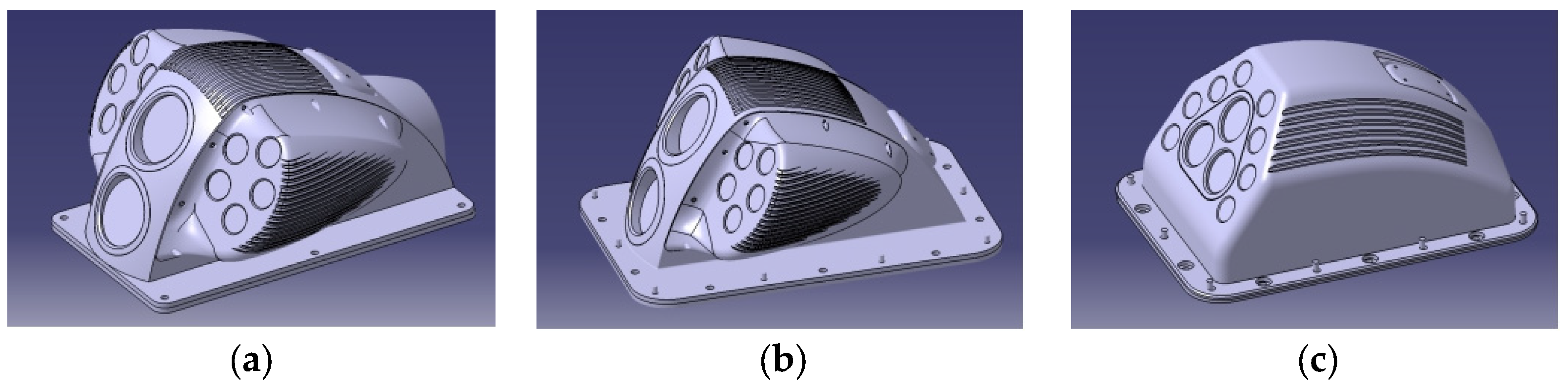
Three device configurations were involved in this calculation (see Figure 1). Among them, configurations 1 and 2 were both C-type buckles with left and right raised ears that were slightly different at the inlet, and configuration 3 was the clean shape of the C-type buckles.
2.2. Calculation Condition
The normal speed range of high-speed trains is about 55~140 m/s. The higher the speed, the greater the aerodynamic load on the device. Therefore, we considered the aerodynamic force on the train at the highest speed. With the viewing window of the device facing the positive airflow direction, the aerodynamic characteristics of the three model configurations at a vehicle speed V = ±110 m/s were investigated, and the force and moment coefficients and surface pressure on the body surface and its ears were mainly calculated. Six calculation conditions were used in total (see Table 1).
2.3. Computational Grid
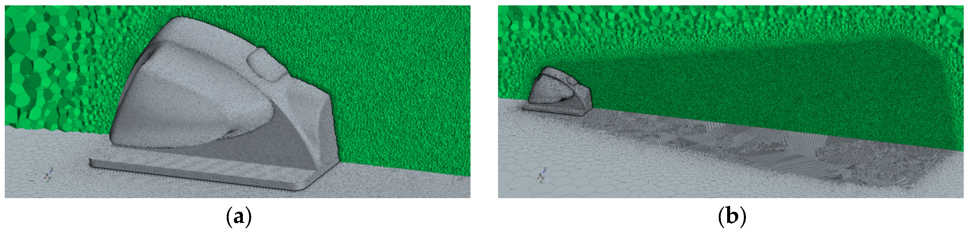
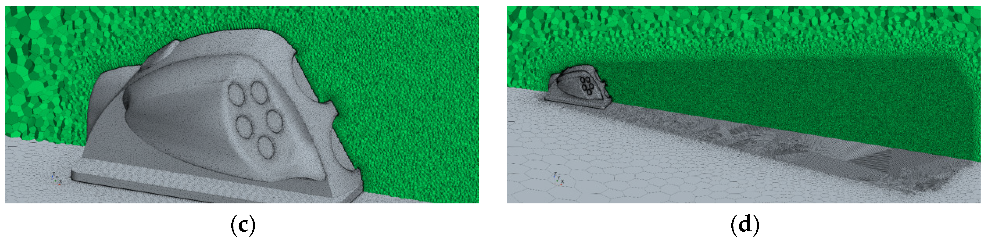
Unstructured grids were used for this investigation. The calculation model is shown in Figure 2. Considering that the device was installed on the top of the train and was far away from the head and tail of the train, the influence of the train shape on the flow field was ignored, and only the installation plane of the device was set as the fixed wall plane and as the boundary condition of the influence of the train roof; that is, the influence of the shape on the flow field could be simplified as the flow around the device installed on the fixed wall plane. Because the device was symmetrical and the incoming flow had no sideslip angle, the semi-model calculation could be adopted, whereby we took a distance that was 20 times the reference distance as the far-field pressure boundary, P = 101,325 Pa, and the temperature was 300 K. The calculation grid is shown in Figure 2. Among the grids, the positive grid quantity of configuration 1 was about 16 million, and the negative grid quantity of the form was about 15 million. The wake area was encrypted according to the different driving directions.
2.4. Control Equations and Discretization Schemes
The train was assumed to operate at a speed of V = 110 m/s and a temperature of T = 300 K (27 °C). At this time, the Mach number of the incoming flow relative to the train was about M = 0.32, which belonged to the subsonic range of aerodynamics. The compressibility of the air needed to be considered, so the complete gas model was adopted. If the length of the device in the x direction was taken as the reference length of the Reynolds number L = 0.5 m, then Re = 3.54 × 10⁶, which belongs to the turbulent flow.
Because the Mach number of the incoming flow was M = 0.32, which belongs to the subsonic category, the air followed the complete gas model, and the Reynolds number corresponding to the flow was about Re = 3.54 × 10⁶. Therefore, the control equation of the problem was the compressible Reynolds average Navier–Stokes equation (RANS equation), in which the shear stress transfer (SST) turbulence model was used to treat the turbulence. The three-dimensional conservative RANS equations follow the computational coordinate system. For the specific meaning of each item, please refer to books on computational fluid mechanics.
The finite volume method was used to discretize the N-S equation [16,17,18], a practical and widely used method in engineering. The bounded central differencing (BCD) scheme was used to discretize the flux terms; with this scheme, we adopted a blended coefficient (φ) to adjust the numerical accuracy and stability. For the present simulation, the coefficient (φ) was set to 0.15 to reduce the numerical dissipation considerably. This calculation is unsteady, and we finally obtained steady results with a high convergence rate. The implicit scheme with dual-time steps was adopted, the physical time step was 0.00005 s, and 10,000-time steps were iteratively calculated.
2.5. Turbulence and Transition Model
Because the Reynolds number of the monitoring device was medium, to accurately evaluate the aerodynamic resistance, the transition impact needed to be considered. Additionally, a large range of separated flows exists when operating high-speed trains. To increase the accuracy of the numerical simulation, we used a coupling γ-Reθ transition model and IDDES method.
The γ-Reθ transition model not only includes the intermission factor transport equation [19,20,21,22], but it also uses the momentum thickness Reynolds number as a transport scalar and establishes the transport equation for it; this allows the momentum thickness Reynolds number of the incoming flow to be used for the boundary layer due to convection, which thus allowed us to obtain the local transition initial momentum thickness Reynolds number. Then, we could judge the beginning of the transition by comparing the Reynolds number of the vortex and momentum thickness. The intermittent factor (γ) and the transport equation of the Reynolds number of the transition initial momentum thickness () was as follows:
where and are the generation and destruction terms of the equation, respectively; is the generation terms of the transport equation; is the Reynolds number of the momentum thickness outside the boundary layer, which is related to the turbulence intensity and pressure gradient of the incoming flow; and is the parameter representing the pressure gradient. Two key factors influence the term and determine the threshold function () at the beginning of the transition and the parameters of the transition region length (). In the upstream laminar flow region, the value is 0. When the Reynolds number () of the ground vortex is greater than 2.193 times the critical momentum thickness Reynolds number (), is activated, the intermittent factor gradually increases, and the and of the flow gradually changes from determining the laminar flow to turbulence. Both parameters are related to the Reynolds number () of the initial momentum thickness of the transition. Langtry successfully associated these two parameters by analyzing many plate test data. These two correlations contain the internal physical mechanism of transition, and many modified versions based on the transition model have modified these two correlations accordingly. The above two transport equations modify the generation and destruction terms of the k equation in the SST model through the intermittent factor, where and represent the generation and destruction terms of the k equation in the SST model, respectively. and represents the generation and destruction terms of the k equation after coupling with the transition model, respectively.
2.6. Combination of IDDES Method and Transition Model
The γ-Reθ model solves the intermission factor γ by adding two transport equations and combines the SST turbulence model by causing γ to act on the generation and destruction terms of the k equation. In terms of form, adding the IDDES method based on the SST model is simpler, and this can be performed by modifying the length scale function of the damage term of the turbulent kinetic energy transport equation in the SST turbulence model. The turbulent kinetic energy equation in the SST model is
where is the damaged item, which should actually be . Because in the RANS model, the equation is finally displayed as , where . For the IDDES method, . To combine the IDDES method with γ-Reθ, if the transition model is combined, it needs to be solved by using γ-Reθ, and the four-equation transition model is obtained by modifying the length scale function of the damage term of the turbulent kinetic energy equation. The turbulent kinetic energy transport equation in the four-equation model is
For the traditional γ-Reθ transition model, in the IDDES framework based on the γ-Reθ transition model, and . So far, whether the pure IDDES method or framework based on γ-Reθ is used, the transition model only needs to be provided, and then the equation can be used.
For details on developing the length-scaling function from DES to IDDES, please refer to the literature. We only provide the calculation of related to the grid scale:
Here, and . is the distance from the wall and is an empirical constant that is independent of the sublattice model and is generally taken as .
is in the form of
Here, , , , and , .
where is the turbulent viscosity coefficient and . is the Karman constant. is the empirical constant, which is taken as 20 in IDDES based on the SST model. is defined as follows:
Here, , and was determined.
2.7. Numerical Validation
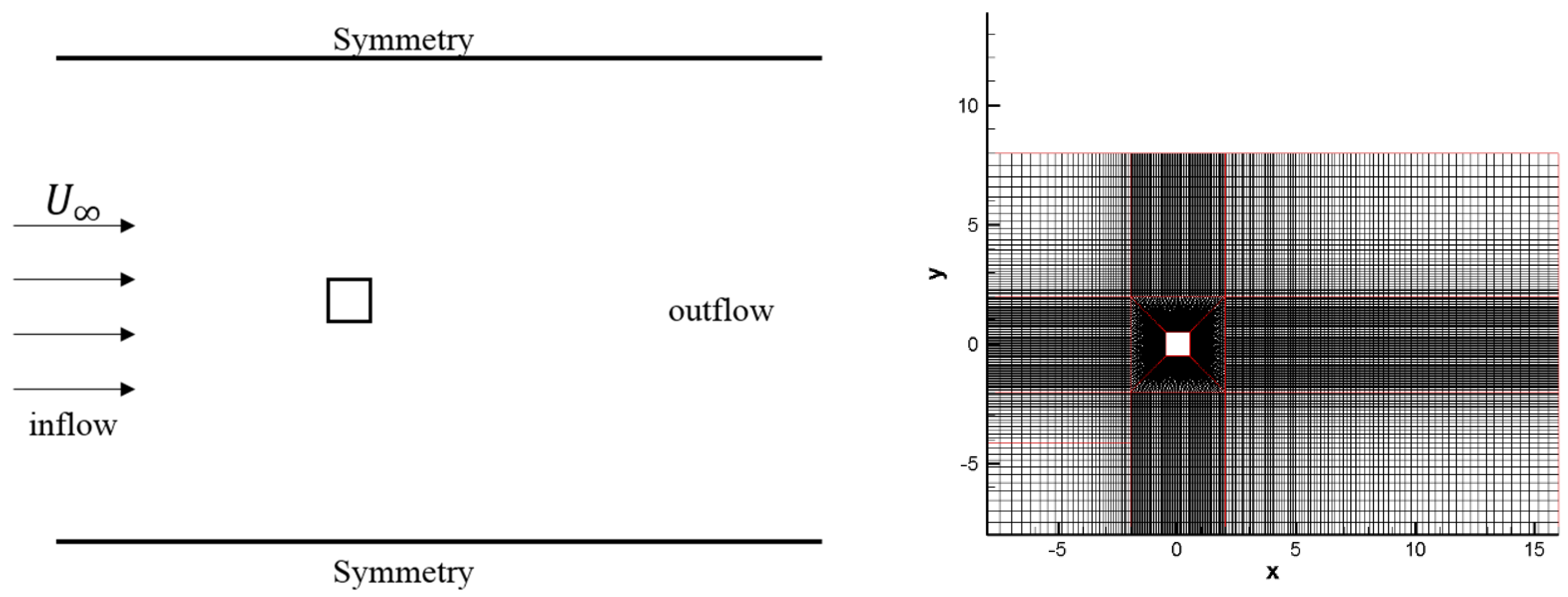
The case of square cylinder flow at a high Reynolds number was adopted to validate the numerical method. The Reynolds number was 2.2 × 10⁴ based on the side length of the square, and the Mach number was 0.2. A set of grids contained 2.8 million cells, refined near the wall to ensure the y+ ≈ 1 for the first grid spacing. The physical time step was 0.005 s, and the Courant number during the inner iteration was 10. Figure 3 illustrates the computational field and grid distribution.
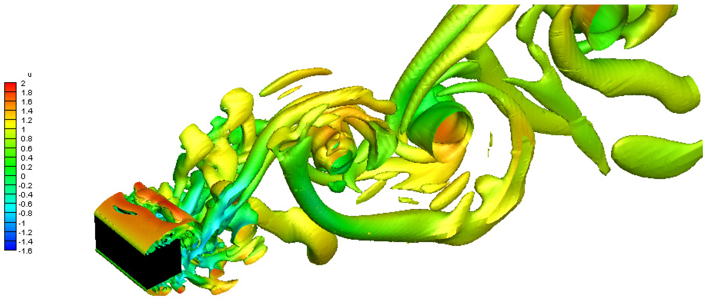
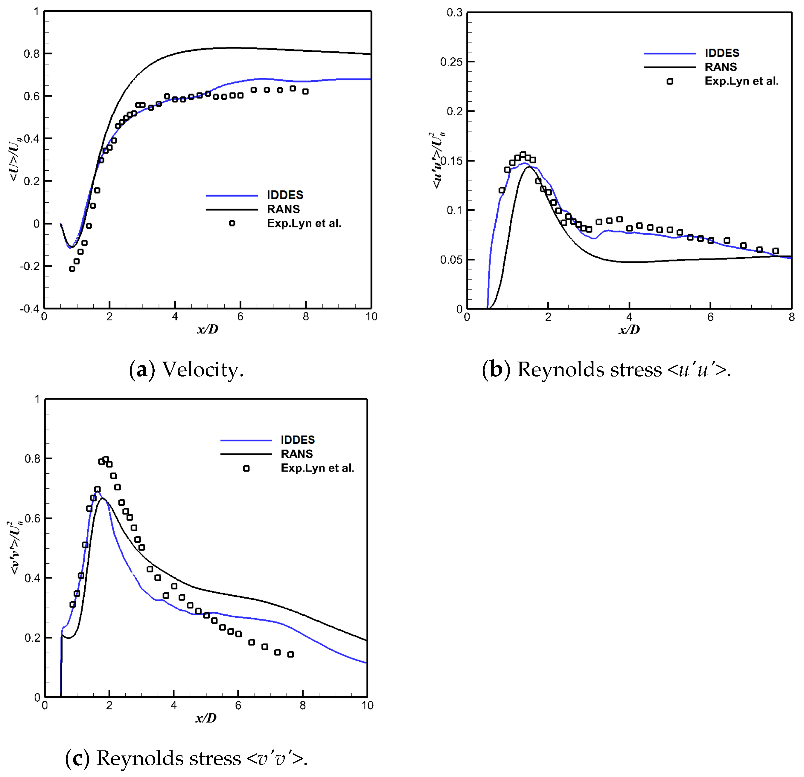
The Q criterion is commonly used to depict the coherent structures of the intricate wake flow. A detailed definition is provided in reference [23]. Figure 4 provides the Q isosurface distribution with a nondimensional Q = 0.45. The large-scale, three-dimensional vortex alternately shed in the wake. The quantitative results are provided and compared with the experiment results in Figure 5, which includes the time-averaged streamwise velocity and the Reynolds stress. The simulation results agreed with the experimental ones well, and we concluded that the numerical IDDES model provided higher numerical accuracy than the RANS model.
3. Result Discussion
3.1. Aerodynamic Comparison
The results of the aerodynamic force and moment coefficient calculations are provided in Table 2, which were nondimensionalized based on the inflow density (ρ), velocity (V), characteristic area, and device length, as defined in Equation (21):
where ρ = 1.225 kg·m3, V = 110 m/s, Sc = 0.149 m2, and Lc = 0.5 m. Because the stress of the components (ears), the moment characteristics, and the other parameters of the swing ears need to be considered, the lift and drag were used for the full-mode results, and all the moments and lateral forces were used for the half-mode integration results.
Because some common characteristics were present in the flow field of the three configurations, we mainly analyzed the aerodynamic characteristics under the two conditions of configuration 1. We only described the conclusions for configurations 2 and 3.
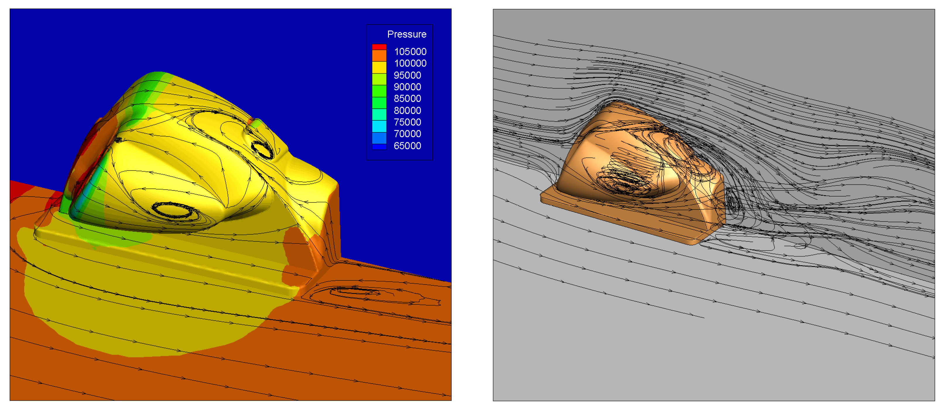
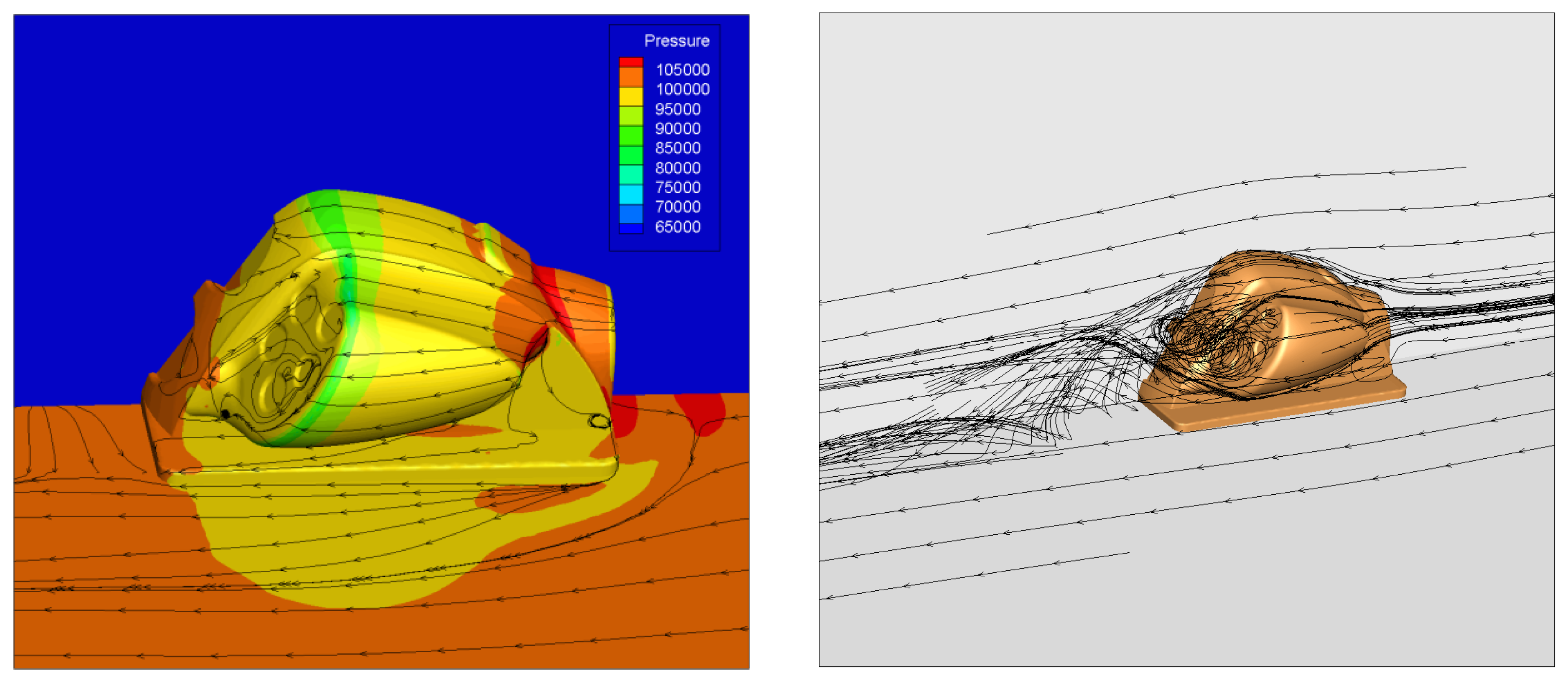
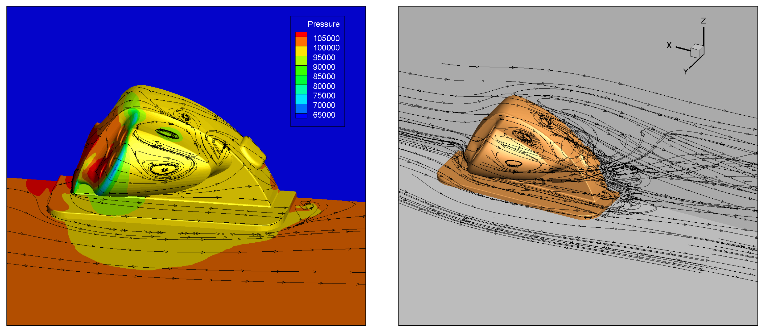
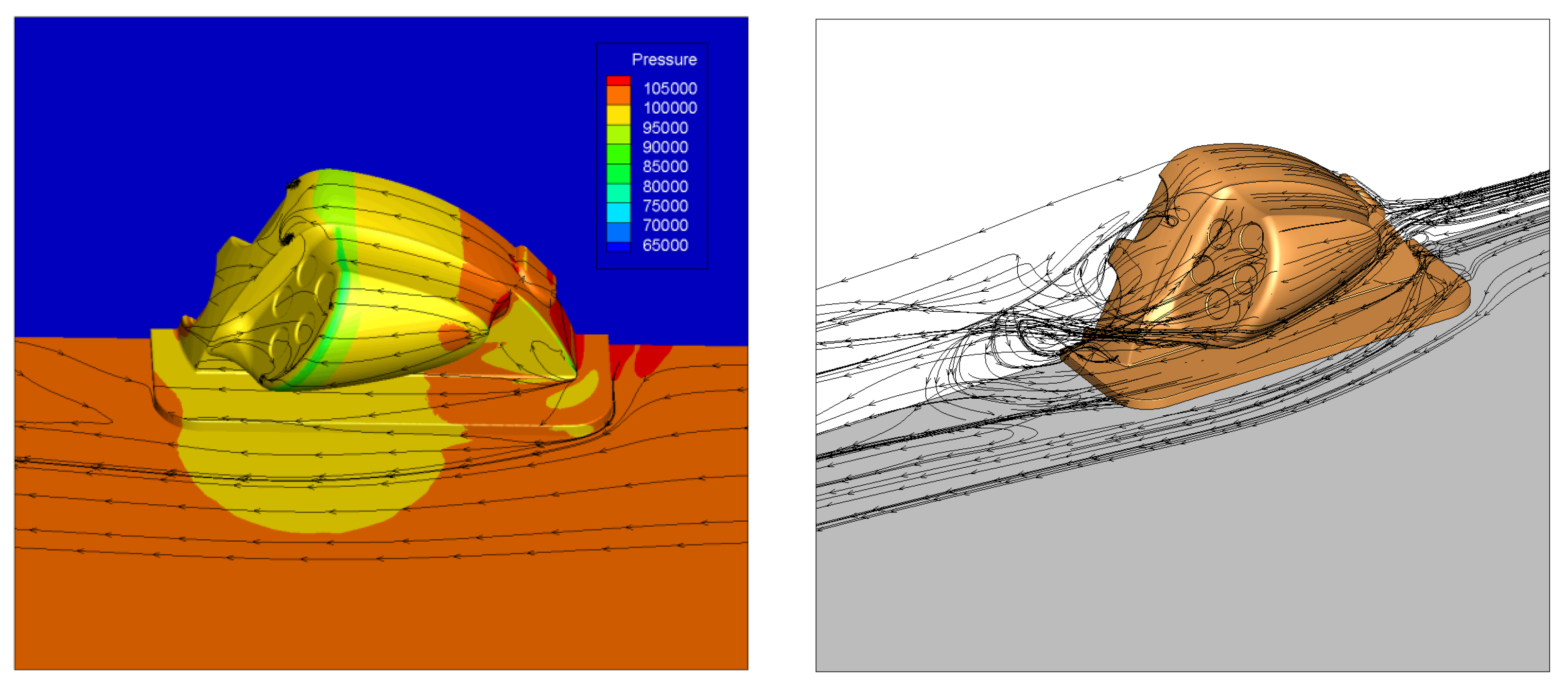
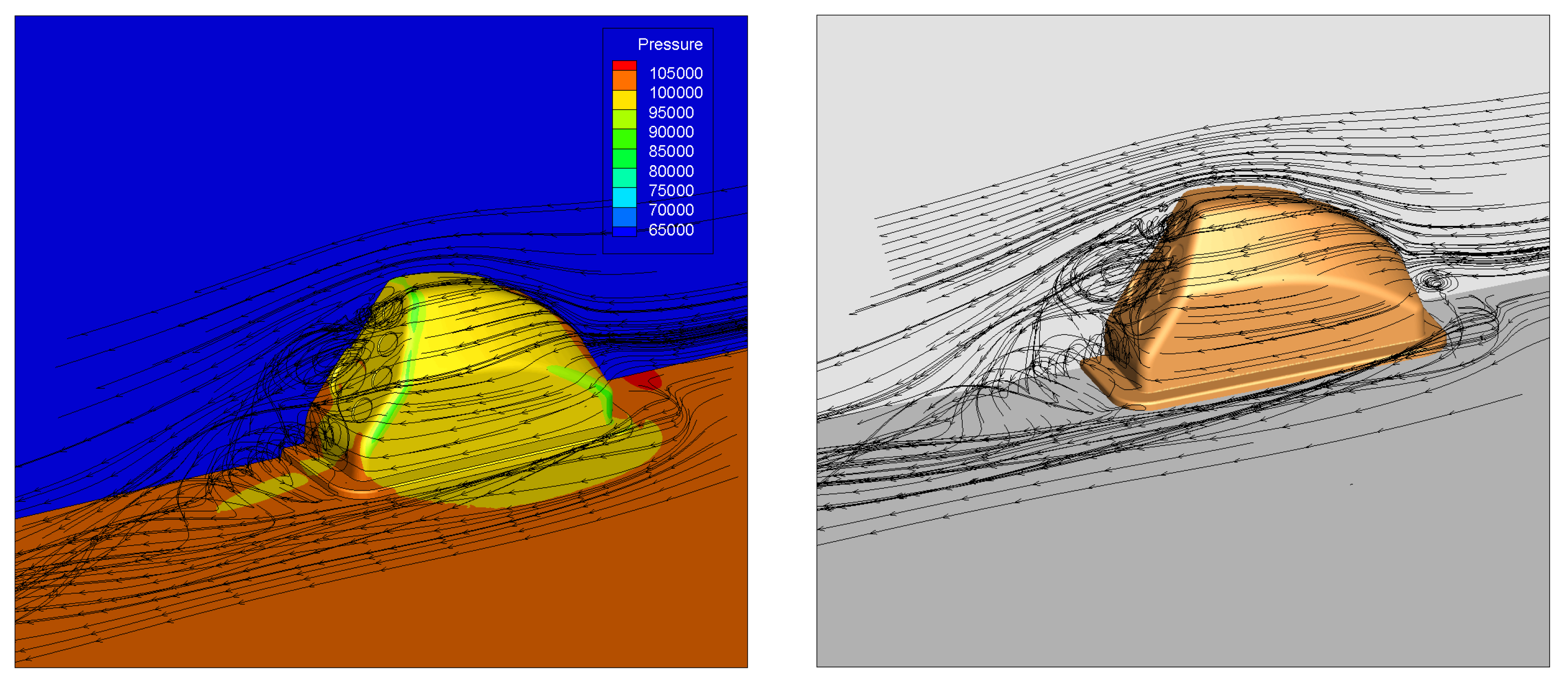
Figure 6, Figure 7, Figure 8, Figure 9, Figure 10 and Figure 11 show the pressure distribution and streamlines on the surface of the device, as well as the off-surface streamlines around the device under different working conditions. An evident high-pressure zone appeared on the windward side because the blockage effect of the device reduced the flow velocity; additionally, the low-pressure belt at the shoulder was induced by the flow acceleration when it bypassed the large-curved corner, and a reverse pressure gradient was formed because of the intense flow acceleration and the relatively higher pressure downstream of the shoulders. Then, the flow separated near the shoulders, forming a recirculation zone on the leeward side. The separation slowed down the pressure recovery and induced a pressure difference between the opposite sides, which contributed to the drag force of the device.
As shown in Figure 6, the area of the high-pressure zone on the windward side of configuration 1 was large under operating conditions. It was mainly distributed in the lower half of the two observation windows and the windward side of the two ears. About 1/3 of the total drag was caused by the two ears. Reducing the windward area of the two ears is appropriate when ignoring other design constraints. For example, increasing the sweep angles of the two sides of the ears can reduce the drag during forward driving. Figure 6 shows three dominant eddies downward from the leeward side of configuration 1 under operating conditions. They formed a large recirculation zone near the leeward side of the ear and the leeward area at the upper part of the inlet and behind the inlet. Therefore, the resistance under condition 1 was large. When driving in the reverse direction (condition 2), a similar pressure distribution existed as when driving in the forward direction. The area of the high-pressure zone at the two ears was smaller than that in condition 1. The relative position of the separation point was behind, and the backflow zone at the leeward side was also smaller. Therefore, the total drag was considerably reduced by about 50% compared with the reduction in the total drag in the forward direction.
The configuration 2 situation was similar to that of configuration 1, and the resistance under the two conditions was equivalent to that of configuration 1. The third configuration was clean and had no strong blocking effect when the ear drove forward. The resistance magnitude of forward and reverse driving was the same, and reverse driving was slightly slower than forward.
The ear of configurations 1 and 2 was subjected to a large negative lift when driving in the forward direction (in modes 1 and 3, respectively). This was because the air separation occurred above the two ears, and the pressure was high, whereas the flow near the ears induced a lower pressure. The pressure difference produced about 0.27 (condition 1) and 0.22 (condition 3) downward resultant force coefficients on a single ear and a remarkable rolling moment. Thus, one must pay considerable attention to the strength of the connection between the ears and the body during the design stage.
3.2. Unsteady Flow Analysis of Wake
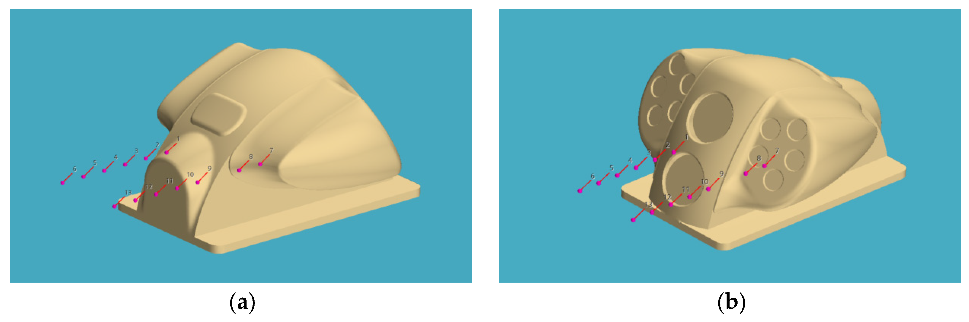
A large, separated flow in the leeward area of the surface-monitoring device on the high-speed train was present. To evaluate its unsteady aerodynamic characteristics, the unsteady aerodynamic characteristics of configuration 1 with a large separation area were analyzed. According to the flow characteristics of the leeward area of the monitoring device, two rows of monitoring points were arranged. One row was on the symmetry plane, starting 10 cm away from the object surface and with an interval of 10 cm from each point, resulting in six monitoring points. The other row was near the Guangyuan glass; it also started 10 cm away from the object’s surface and had an interval of 10 cm from each point, resulting in seven monitoring points. See Figure 12 for the detailed layout.
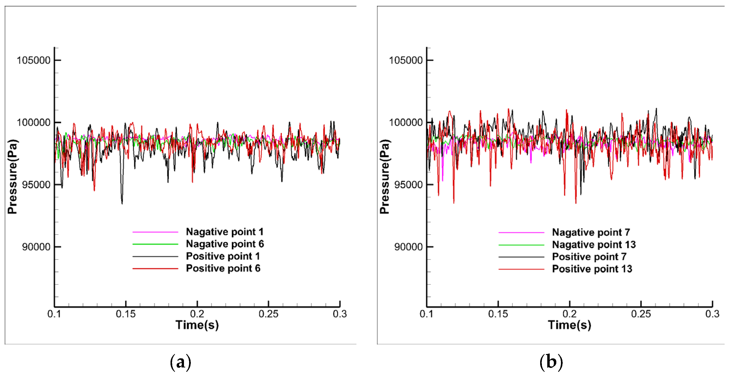
Figure 13 compares the pressure pulsations at different monitoring points during positive and negative operations. Figure 13a shows that the pressure pulsation at the center line of the forward operation was smaller than that of the negative operation, whether the point near the wall (point 1) or far away from the wall (point 6) was used. Figure 13b shows that the contrast between the positive and negative movement at the right monitoring point was consistent with the law at the center line. The overall pressure fluctuation of the right monitoring point was larger than that of the monitoring point at the center line. This was mainly because the right monitoring point was closer to the boundary of the external high-speed airflow and the airflow stagnation zone at the rear of the monitoring device and because the relationship between the mass transfer effect between different areas was more intense.
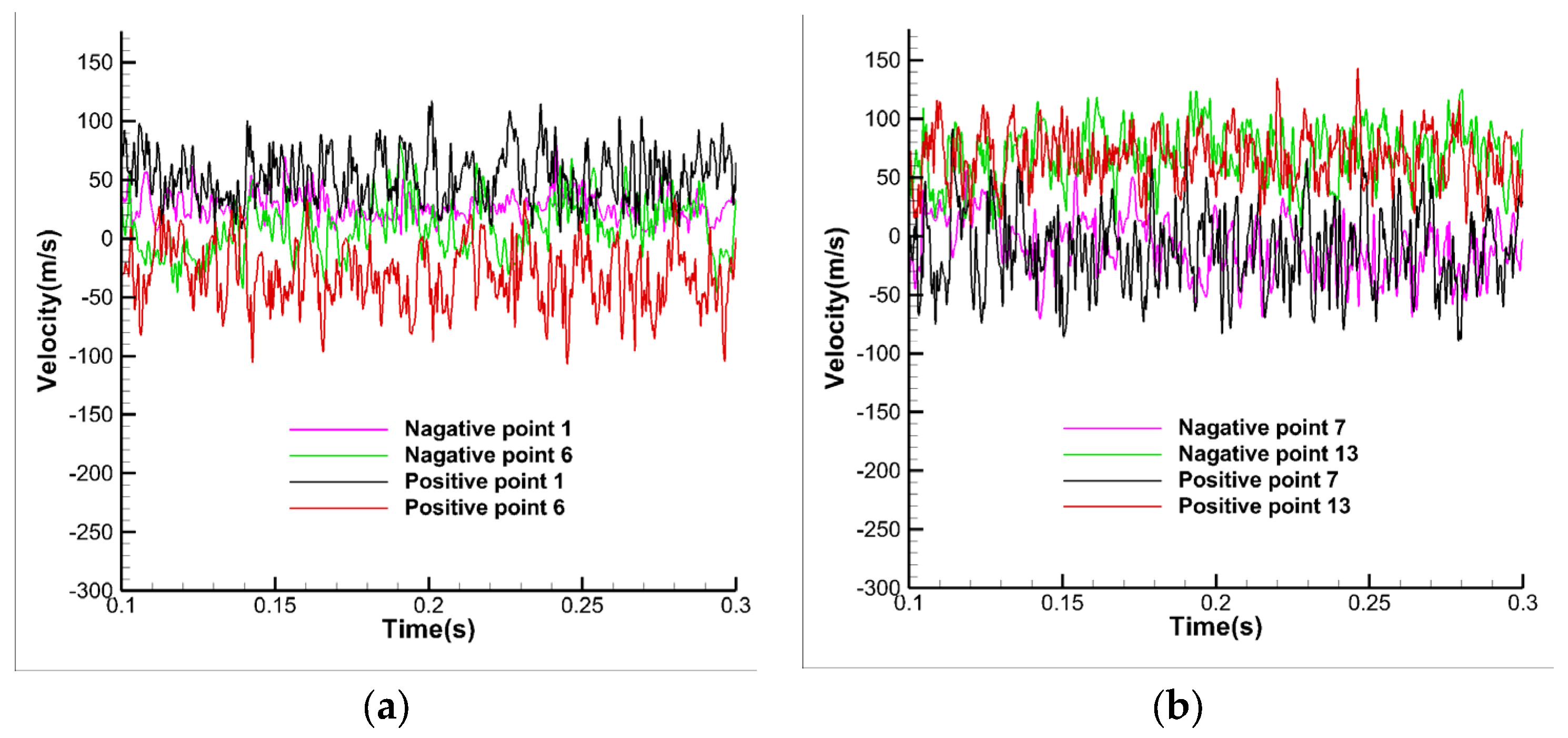
Figure 14 compares the pressure and velocity combinations at different monitoring points during the positive and negative operations. Figure 14a shows that at the center line, a large positive velocity was present at the point close to the wall (point 1), and a large reverse velocity was present at the point far away from the wall (point 6), which indicates that a small separation zone was present at the center line. During the reverse operation, a large positive velocity was also present at the point near the wall (point 1). In contrast, the velocity at the point far away from the wall (point 6) was 0, which indicated that this area was the velocity stagnation region. This could be mutually verified with the flow field structure shown in Figure 13. Figure 14a shows that the pressure pulsation at the monitoring point on the right side was consistent with the law of the pressure pulsation at the monitoring point during the positive and negative operation, both of which formed reflux near the wall; additionally, the velocity in the area far away from the wall was consistent with the outflow, which indicated that a certain separation flow area was also present on the right side, which is consistent with the spatial streamline shown in Figure 6 and Figure 7.
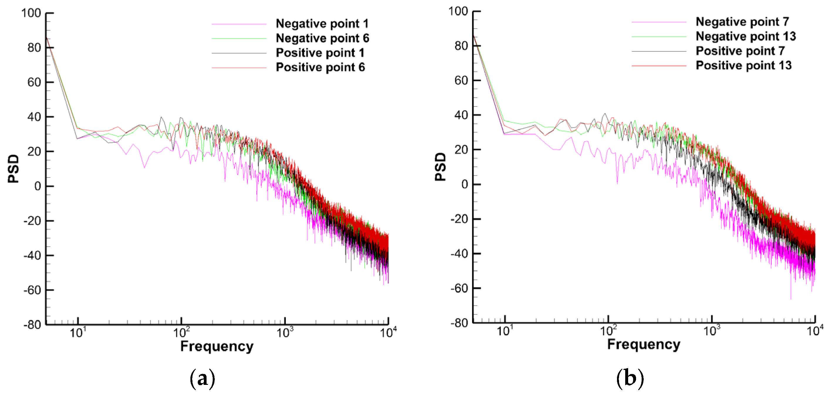
A power spectrum density (PSD) analysis was conducted to analyze the pressure time history. Figure 15 compares the power density spectra, whereby the pressure fluctuations at different monitoring points during the positive and negative operations are compared. The pressure fluctuation at the monitoring points in the wake area had no obvious peak value, and the PSD values of the points (points 1 and 7) close to the wall during the negative operation were considerably reduced, which showed that the flow near the wall in the leeward area was relatively stable during the negative operation.
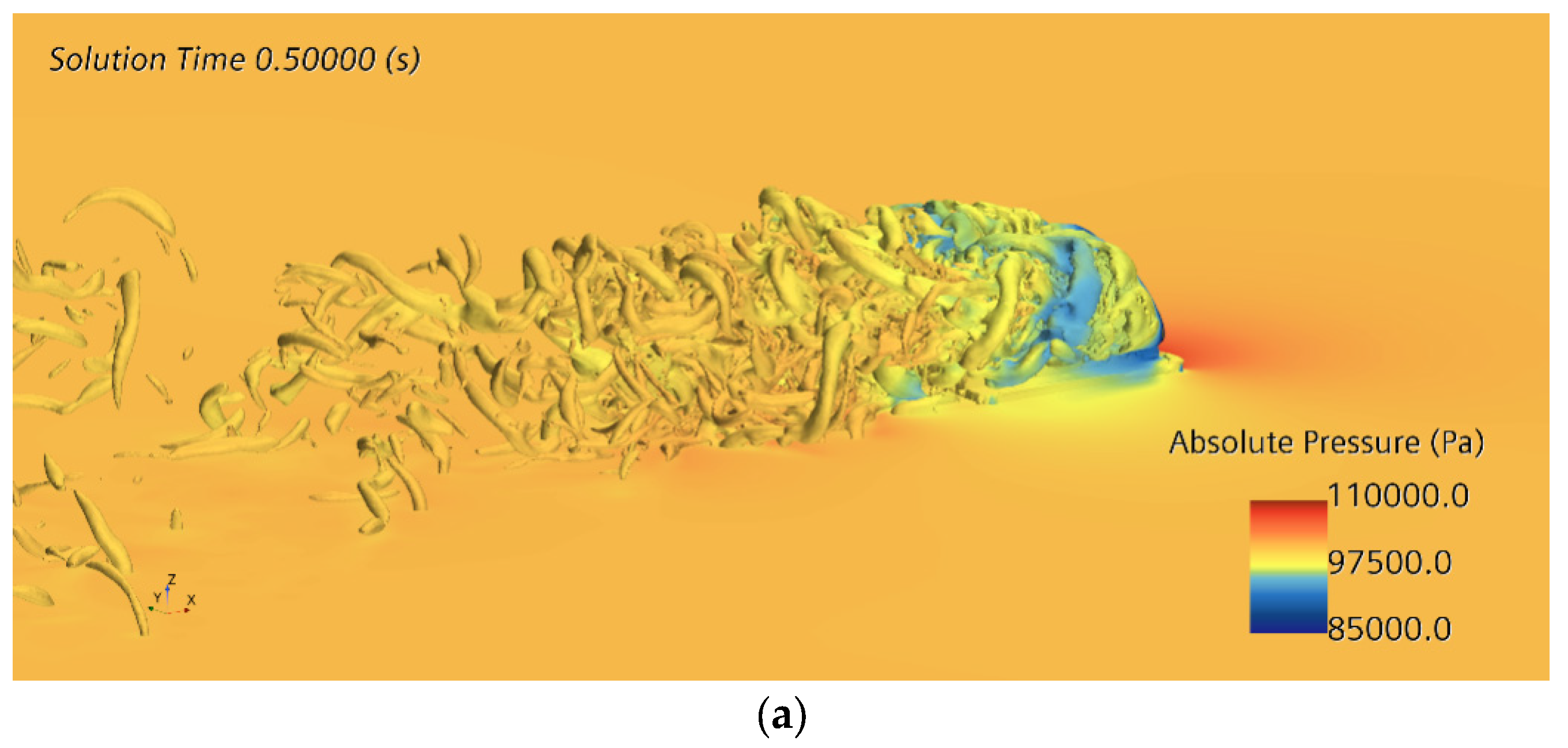
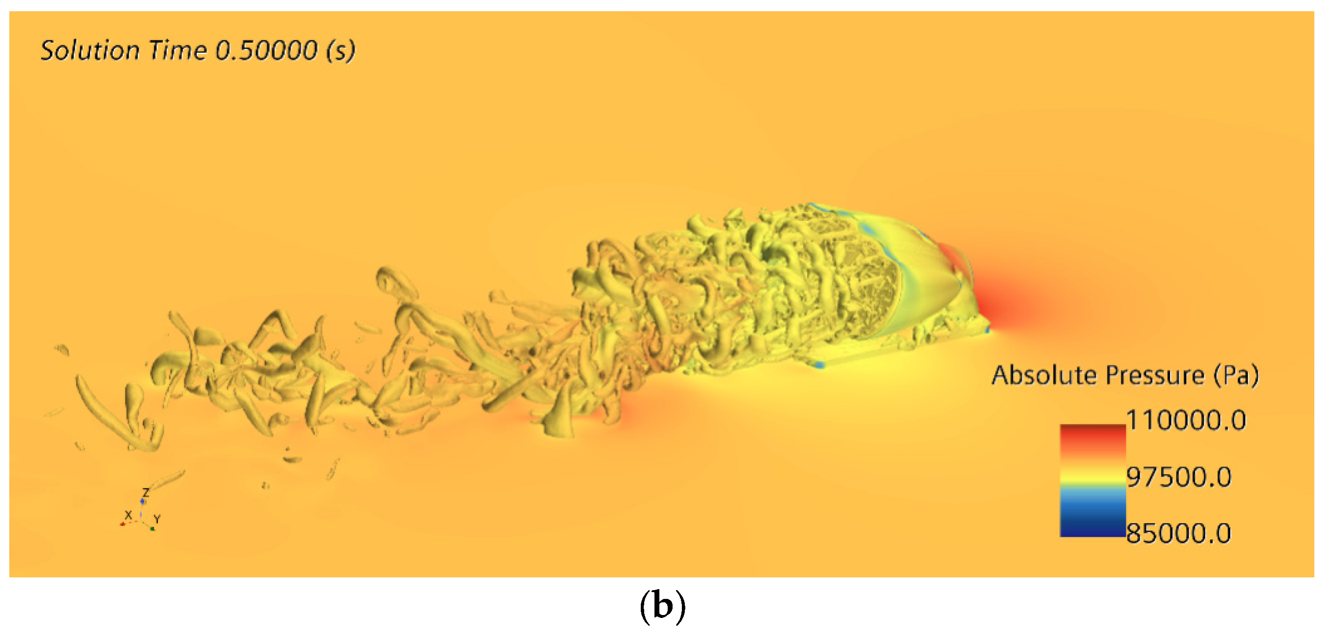
Figure 16 shows the characteristics of the wake separation using the Q isosurface colored according to the pressure. More abundant leeward vortex structures were present in the forward operation, and the influence of the separation zone was also wider, which was consistent with the performance of the overall aerodynamic drag.
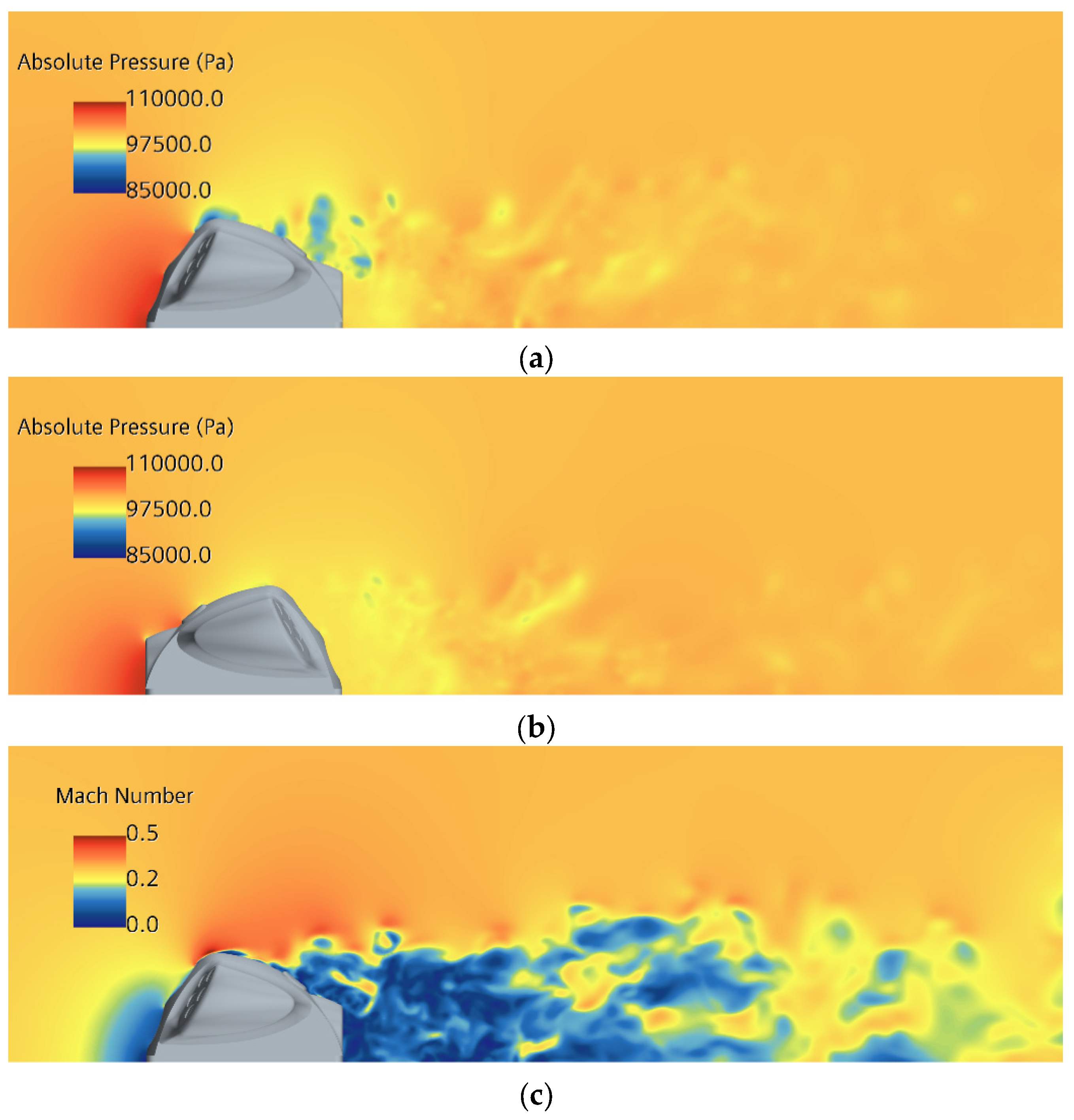
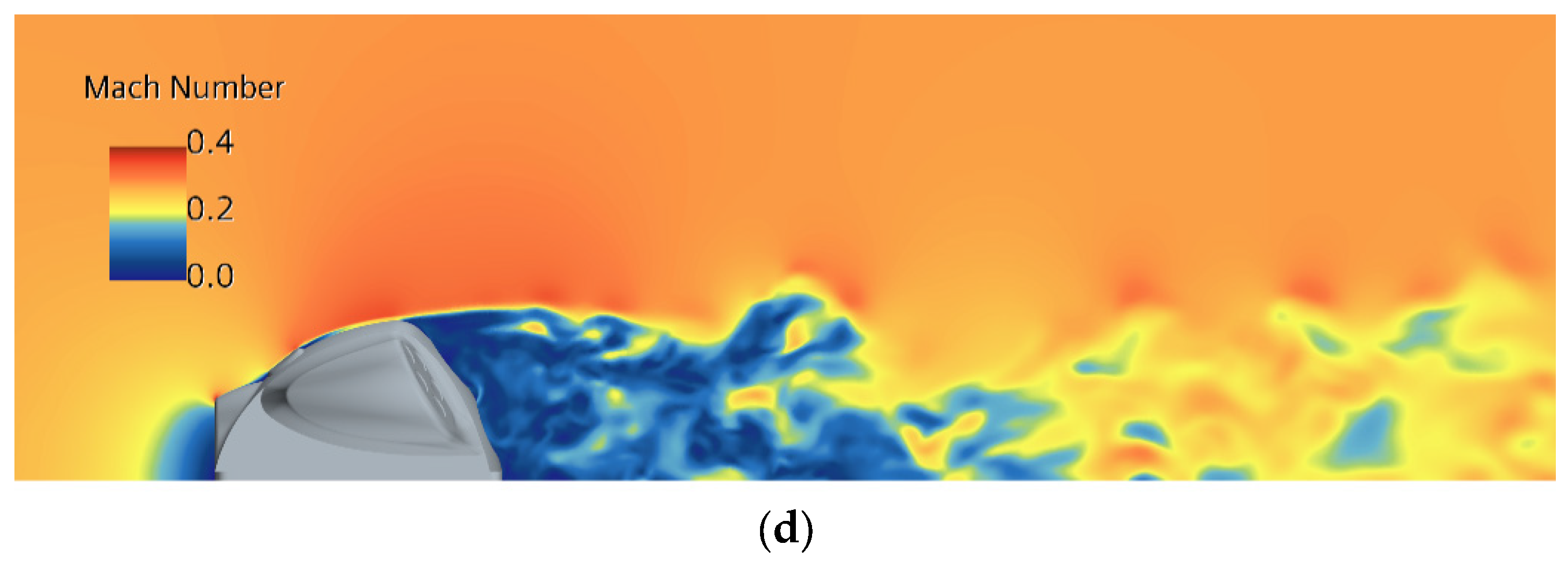
Figure 17 compares the symmetry plane’s pressure and Mach number distribution under different operation conditions. The separation area and influence range of the wake flow during the forward operation was larger than those during the negative operation, and the wake flow was partially far away from the top of the train, which was also the reason for the greater resistance during the forward operation.
4. Conclusions
Numerical simulation research on the operation-condition monitoring device of a high-speed train was conducted. The calculation accuracy was increased by using the IDDES method. By conducting an analysis of the aerodynamic force, surface flow pattern, and space wake structure, the following conclusions were obtained:
- (1)
- The windward side of the detection device experienced positive pressure, and the sideline and leeward sides experienced negative pressure. Increasing the fillet radius of the sideline can appropriately reduce the aerodynamic resistance.
- (2)
- The shaping of the downstream flow in the leeward area can effectively reduce the resistance of the monitoring device. The resistance of configurations 1 and 2 in the reverse direction was about 1/2 of that in the forward direction, and the resistance of configurations 3 in the forward and reverse directions was the same. The streamlined upwind surface was conducive to reducing the scope of the leeward separation area and the amplitude of the pressure fluctuation in the leeward area and thus reduced the resistance;
- (3)
- The monitoring device had a certain height and formed a vortex on its leeward side when the train was running at high speed. From the results of the analysis on the pressure monitoring, we found that the separated airflow did not have an obvious dominant frequency and energy peak, and the possibility of resonance damage occurring to the following parts, such as the top of the train, was small.
Author Contributions
Methodology, B.L., X.W. and N.X.; Software, B.L. and X.W.; Validation, X.W. and N.X.; Formal analysis, Y.T. and N.X.; Investigation, B.L. and J.W.; Resources, J.W.; Data curation, J.W.; Writing—original draft, Y.T. All authors have read and agreed to the published version of the manuscript.
Funding
This work was funded by the National Natural Science Foundation of China, grant number 11372337.
Conflicts of Interest
The authors declare no conflict of interest.
References
- Zhou, N.; Yang, W.; Liu, J.; Zhang, W.; Wang, D. Investigation of a pantograph-catenary monitoring system using condition-based pantograph recognition. Sci. Sin. Technol. 2021, 51, 23–34. [Google Scholar]
- Xiukun, W.; Da, S.; Dehua, W.; Xiaomeng, W.; Siyang, J.; Ziming, Y. A survey of the application of machine vision in rail transit system inspection. Control. Decis. 2021, 36, 257–282. [Google Scholar]
- Han, Z.; Liu, Z.; Zhang, G.; Yang, H.M. Overview of non-contact image detection technology for pantograph-catenary monitoring. J. China Railw. Soc. 2013, 35, 40–47. [Google Scholar]
- Hongqi, T. Train aerodynamics; China Railway Press: Beijing, China, 2007. [Google Scholar]
- Zhenxu, S.; Yongfang, Y.; Dilong, G.; Guowei, Y.; Shuanbao, Y.; Ye, Z.; Dawei, C.; Guibo, L.; Keming, S.; Ling, J. Research progress in aerodynamic optimization of high-speed trains. Chin. J. Theor. Appl. Mech. 2021, 53, 51–74. [Google Scholar]
- Jiqiang, N.; Xifeng, L.; Dan, Z. Equipment cabin aerodynamic performance of electric multiple unit going through tunnel by dynamic model test. J. Zhejiang Univ. Eng. Sci. 2016, 50, 1258–1265. [Google Scholar]
- Liu, T.; Chen, Z.; Zhou, X.; Zhang, J. A CFD analysis of the aerodynamics of a high-speed train passing through a windbreak transition under crosswind. Eng. Appl. Comput. Fluid Mech. 2018, 12, 137–151. [Google Scholar] [CrossRef] [Green Version]
- Xu, J.L.; Sun, J.C.; Mei, Y.G.; Wang, R.L. Numerical Simulation on crossing pressure wave characteristics of two high-speed trains in tunnel. J. Vib. Shock. 2016, 35, 184–191. [Google Scholar]
- Weibin, M.A.; Qianli, Z.H.N.; Yanqing, L.I. Study evolvement of high-speed railway tunnel aerodynamic effect in China. J. Traffic Transp. Eng. 2012, 12, 25–32. [Google Scholar]
- Niu, J.Q.; Zhou, D.; Liu, T.H.; Liang, X.F. Numerical simulation of aerodynamic performance of a couple multiple units high-speed train. Veh. Syst. Dyn. 2017, 55, 681–703. [Google Scholar] [CrossRef]
- Kim, H.; Hu, Z.; Thompson, D. Effect of cavity flow control on high-speed train pantograph and roof aerodynamic noise. Railw. Eng. Sci. 2020, 28, 54–74. [Google Scholar] [CrossRef] [Green Version]
- Ko, Y.Y.; Chen, C.H.; Hoe, T.; Wang, S.T. Field measurements of aerodynamic pressures in tunnels induced by high speed trains. J. Wind Eng. Ind. Aerodyn. 2012, 100, 19–29. [Google Scholar] [CrossRef]
- Yundong, H.; Dawei, C.; Peng, L. Air distribution simulation study of EMU equipment bay under passing by each other on open track. Railw. Locomot. Car 2013, 33, 22–26. [Google Scholar]
- Zhu, C.; Hemida, H.; Flynn, D.; Baker, C.; Liang, X.; Zhou, D. Numerical simulation of the slipstream around a high-speed train with pantograph system. J. Railw. Sci. Eng. 2016, 13, 1447–1456. [Google Scholar]
- Wang, S.; Bell, J.R.; Burton, D.; Herbst, A.H.; Sheridan, J.; Thompson, M.C. The performance of different turbulence models (URANS, SAS and DES) for predicting high-speed train slipstream. J. Wind Eng. Ind. 2017, 165, 46–57. [Google Scholar] [CrossRef]
- Barman, P.C. Introduction to computational fluid dynamics. Int. J. Inf. Sci. Comput. 2016, 3, 117–120. [Google Scholar] [CrossRef]
- Hill, D.J.; Pantano, C.; Pullin, D.I. Large-eddy simulation and multiscale modeling of a Richtmyer-Meshkov instability with reshock. J. Fluid Mech. 2006, 557, 29–61. [Google Scholar] [CrossRef] [Green Version]
- Baorui, F. Aero-Configuration Design of Aero Plan; Beijing Aviation Industry Publishing Company: Beijing, China, 1997. (In Chinese) [Google Scholar]
- Viswanathan, A.; Squires, K.D.; Forsythe, J.R. Detached-Eddy Simulation around a forebody at high angle of attack. In AIAA Aerospace Sciences Meeting; AIAA Paper 2003-0263; AIAA: Reston, VA, USA, 2003. [Google Scholar]
- Forsythe, J.R.; Squires, K.D.; Wurtzler, K.E.; Spalart, P.R. Detached-eddy simulation of the F-15E at high alpha. In AIAA Aerospace Sciences Meeting; AIAA Paper 2002-0591; AIAA: Reston, VA, USA, 2002. [Google Scholar]
- Morton, S.A.; Steenman, M.B.; Cummings, R.M.; Forsythe, J.R. DES grid resolution issues for vertical flows on a delta wing and an F-18C. In 41st Aerospace Sciences Meeting and Exhibit; AIAA Paper 2003-1103; AIAA: Reston, VA, USA, 2003. [Google Scholar]
- Denning, R.M.; Allen, J.E.; Armstrong, F.W. The broad delta airliner. Aeronaut. J. 2003, 107, 547–558. [Google Scholar] [CrossRef]
- Jeong, J.; Hussain, F. On the identification of a vortex. J. Fluid Mech. 1995, 285, 69–94. [Google Scholar] [CrossRef]
- Lyn, D.A.; Einav, S.; Rodi, W. A laser-Doppler velocimetry study of ensemble-averaged characteristics of the turbulent near wake of a square cylinder. J. Fluid Mech. 1995, 304, 285–319. [Google Scholar] [CrossRef]
Figure 1.
Outline diagram of the monitoring device; (a) Configuration 1; (b) Configuration 2; (c) Configuration 3.
Figure 1.
Outline diagram of the monitoring device; (a) Configuration 1; (b) Configuration 2; (c) Configuration 3.

Figure 2.
Computing grid; (a) Grid near the wall; positive operation: condition 1; (b) Grid far field; positive operation: condition 1; (c) Grid near the wall; negative operation: condition 2; (d) Grid far-field; negative operation: condition 2.
Figure 2.
Computing grid; (a) Grid near the wall; positive operation: condition 1; (b) Grid far field; positive operation: condition 1; (c) Grid near the wall; negative operation: condition 2; (d) Grid far-field; negative operation: condition 2.


Figure 3.
Computational field (left) and grid distribution (right) of the square cylinder flow.

Figure 4.
Q isosurface of the square cylinder flow.

Figure 5.
The time averaged results along the centerline of square cylinder flow [24].
Figure 5.
The time averaged results along the centerline of square cylinder flow [24].

Figure 6.
Condition 1 surface and space streamline.

Figure 7.
Condition 2 surface and space streamline.

Figure 8.
Condition 3 surface and space streamline.

Figure 9.
Condition 4 surface and space streamline.

Figure 10.
Condition 5 surface and space streamline.

Figure 11.
Condition 6 surface and space streamline.

Figure 12.
Distribution of monitoring points in the wake area of the detection device; (a) Positive operation (condition 1); (b) Negative operation (condition 2).
Figure 12.
Distribution of monitoring points in the wake area of the detection device; (a) Positive operation (condition 1); (b) Negative operation (condition 2).

Figure 13.
Comparison of pressure at different detection points; (a) Centerline detection point; (b) Right detection point.
Figure 13.
Comparison of pressure at different detection points; (a) Centerline detection point; (b) Right detection point.

Figure 14.
Comparison of velocity at different detection points (a) Centerline detection point; (b) Right detection point.
Figure 14.
Comparison of velocity at different detection points (a) Centerline detection point; (b) Right detection point.

Figure 15.
Comparison of power density spectra of pressure fluctuation at different detection points; (a) Centerline detection point; (b) Right detection point.
Figure 15.
Comparison of power density spectra of pressure fluctuation at different detection points; (a) Centerline detection point; (b) Right detection point.

Figure 16.
Q isosurface of wake under different operating conditions; (a) Positive operation; (b) Negative operation.
Figure 16.
Q isosurface of wake under different operating conditions; (a) Positive operation; (b) Negative operation.


Figure 17.
Comparison of pressure and Mach number distribution on symmetry plane under different operating conditions; (a) Pressure distribution during positive operation; (b) Pressure distribution during negative operation; (c) Mach number during positive operation (d) Mach number during negative operation.


Table 1.
Working condition comparison table.
| Working Condition | Model | Velocity |
|---|---|---|
| 1 | 1 | 110 m/s |
| 2 | 1 | −110 m/s |
| 3 | 2 | 110 m/s |
| 4 | 2 | −110 m/s |
| 5 | 3 | 110 m/s |
| 6 | 3 | −110 m/s |
Table 2.
Force and moment coefficients for the three grids used in the convergence study.
| Working Condition | Component | Cx | Cy | Cz | mx | my | mz |
|---|---|---|---|---|---|---|---|
| 1 | body | −0.227 | 0.302 | 0.426 | 0.0159 | −0.0147 | 0.0114 |
| ear | −0.141 | 0.559 | −0.272 | −0.1083 | 0.0170 | 0.0389 | |
| total | −0.369 | 0.862 | 0.154 | −0.0924 | 0.0024 | 0.0503 | |
| 2 | body | 0.142 | 0.204 | 0.356 | 0.0109 | −0.0071 | −0.0096 |
| ear | 0.056 | 0.446 | −0.026 | −0.0650 | 0.0134 | 0.0176 | |
| total | 0.197 | 0.650 | 0.330 | −0.0542 | 0.0063 | 0.0080 | |
| 3 | body | −0.263 | 0.290 | 0.529 | 0.0491 | −0.0101 | 0.0205 |
| ear | −0.106 | 0.582 | −0.215 | −0.1065 | 0.0259 | 0.0435 | |
| total | −0.368 | 0.872 | 0.314 | −0.0574 | 0.0158 | 0.0639 | |
| 4 | body | 0.157 | 0.186 | 0.415 | 0.0315 | −0.0350 | −0.0078 |
| ear | 0.062 | 0.420 | −0.050 | −0.0638 | 0.0165 | 0.0197 | |
| total | 0.219 | 0.606 | 0.365 | −0.0322 | −0.0183 | 0.0120 | |
| 5 | body | −0.195 | 0.836 | 0.640 | −0.0446 | 0.0007 | 0.0540 |
| 6 | body | 0.193 | 0.687 | 0.545 | −0.0286 | −0.0069 | −0.0143 |
Note: (1) The moment reference point is the origin of the digital-analog coordinate system; (2) All moments and lateral forces were calculated with a half model to represent the stress of parts (ears) accurately.
Disclaimer/Publisher’s Note: The statements, opinions and data contained in all publications are solely those of the individual author(s) and contributor(s) and not of MDPI and/or the editor(s). MDPI and/or the editor(s) disclaim responsibility for any injury to people or property resulting from any ideas, methods, instructions or products referred to in the content. |
© 2023 by the authors. Licensee MDPI, Basel, Switzerland. This article is an open access article distributed under the terms and conditions of the Creative Commons Attribution (CC BY) license (https://creativecommons.org/licenses/by/4.0/).
Share and Cite
MDPI and ACS Style
Li, B.; Wang, X.; Wu, J.; Tao, Y.; Xiong, N. Aerodynamic Characteristics Analysis of Rectifier Drum of High-Speed Train Environmental Monitoring Devices. Appl. Sci. 2023, 13, 7325. https://0-doi-org.brum.beds.ac.uk/10.3390/app13127325
AMA Style
Li B, Wang X, Wu J, Tao Y, Xiong N. Aerodynamic Characteristics Analysis of Rectifier Drum of High-Speed Train Environmental Monitoring Devices. Applied Sciences. 2023; 13(12):7325. https://0-doi-org.brum.beds.ac.uk/10.3390/app13127325
Chicago/Turabian StyleLi, Baowang, Xiaobing Wang, Junqiang Wu, Yang Tao, and Neng Xiong. 2023. "Aerodynamic Characteristics Analysis of Rectifier Drum of High-Speed Train Environmental Monitoring Devices" Applied Sciences 13, no. 12: 7325. https://0-doi-org.brum.beds.ac.uk/10.3390/app13127325
Note that from the first issue of 2016, this journal uses article numbers instead of page numbers. See further details here.