Bearing Fault Diagnosis Method Based on Deep Learning and Health State Division

Abstract

As a key component of motion support, the rolling bearing is currently a popular research topic for accurate diagnosis of bearing faults and prediction of remaining bearing life. However, most existing methods still have difficulties in learning representative features from the raw data. In this paper, the Xi’an Jiaotong University (XJTU-SY) rolling bearing dataset is taken as the research object, and a deep learning technique is applied to carry out the bearing fault diagnosis research. The root mean square (RMS), kurtosis, and sum of frequency energy per unit acquisition period of the short-time Fourier transform are used as health factor indicators to divide the whole life cycle of bearings into two phases: the health phase and the fault phase. This division not only expands the bearing dataset but also improves the fault diagnosis efficiency. The Deep Convolutional Neural Networks with Wide First-layer Kernels (WDCNN) network model is improved by introducing multi-scale large convolutional kernels and Gate Recurrent Unit (GRU) networks. The bearing signals with classified health states are trained and tested, and the training and testing process is visualized, then finally the experimental validation is performed for four failure locations in the dataset. The experimental results show that the proposed network model has excellent fault diagnosis and noise immunity, and can achieve the diagnosis of bearing faults under complex working conditions, with greater diagnostic accuracy and efficiency.

1. Introduction

The bearing is one of the most critical parts of rotating machinery. If a fault occurs in use, it will seriously affect the normal operation of mechanical equipment, causing huge losses and disasters. Therefore, bearing fault diagnosis is an essential step for the normal operation of modern rotating machinery. Research on bearing diagnosis methods and fault mechanisms to ensure the normal operation of bearings has always been a key issue of concern for domestic and foreign experts. Nowadays, machinery system health monitoring has stepped into the era of big data, which is manifested in the use of sensors to obtain monitoring sample data, deep learning to accumulate training experience as the main technical means, and intelligent judgment of machinery health status as the ultimate goal, to ensure the reliability of equipment operation and promote efficient production.

At present, bearing fault diagnosis technologies mainly include vibration analysis, acoustic analysis, oil sample analysis, temperature analysis, and voltage current detection [1].

The vibration analysis method is a widely used diagnosis method, in which the vibration signal can be measured online and combined with deep learning technology feature extraction to determine the early failure type of the bearing. However, due to the high cost of data acquisition, the need for storage and transmission technology to be developed, and other reasons, the typical vibration signal fault diagnosis dataset is extremely scarce, which seriously restricts the theoretical research and engineering application of mechanical equipment health management technology and fault diagnosis.

In the past 20 years, the research on deep learning fault diagnosis of bearing vibration signals has mainly included the following three aspects:

(1)

Selection of datasets

The Western Reserve University dataset [2] is one of the most studied datasets for bearing fault diagnosis by many scholars. However, single dataset research also hinders the research of bearing fault diagnosis algorithms. More and more scholars are also working on newer fault diagnosis datasets. The Prognostics and Health Management (PHM) 2012 bearing full-cycle life dataset (FEMTO-ST) [3] is the most used dataset in full-cycle life prediction studies, but the disadvantages of this dataset are that the failure location is not given and the sampling duration is only 0.1 s. The frequency resolution is low and it is not possible to perform fault diagnosis classification studies. The University of Cincinnati bearing dataset [4], which contains the full cycle life and failure location of bearings, is generally used for bearing remaining life prediction studies. It is also used by more and more scholars in the field of fault classification. However, this dataset was only obtained under a single operating condition with constant values of both rotational speed and radial load, and the sample size is small. Moreover, many scholars are discouraged by the long time of disclosure and the large amount of data.

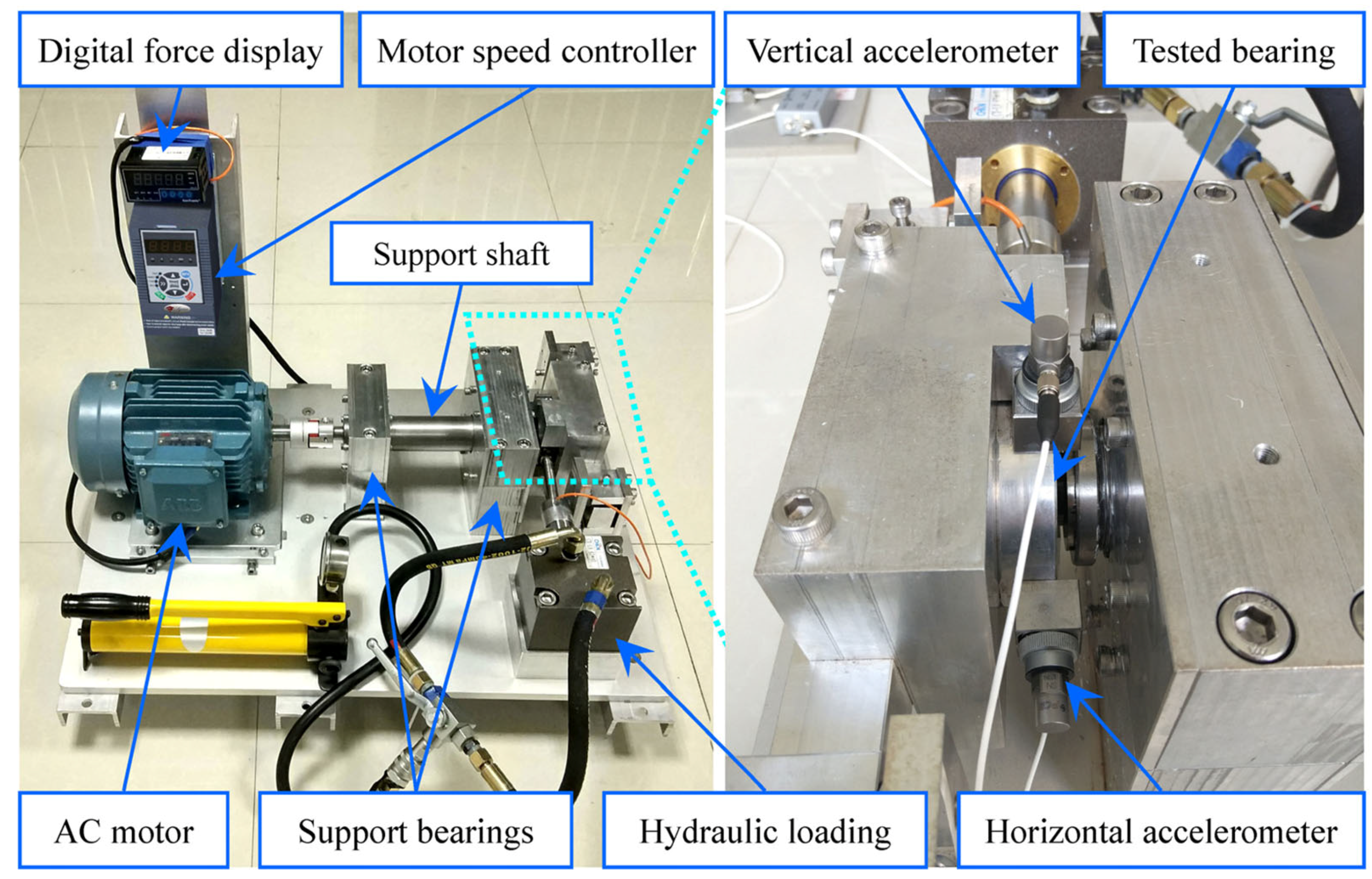
Professor Lei Yaguo’s team in the School of Mechanical Engineering, at Xi’an Jiaotong University, publicly released the XJTU-SY dataset [5], which contains the full life-cycle vibration signals of 15 rolling bearings under three working conditions. The motor speed for condition 1 is 2100 r/min and the radial force is 12 KN; the speed for condition 2 is 2250 r/min and the radial force is 11 KN; the speed for condition 3 is 2400 r/min and the radial force is 10 KN. The dataset is clearly labeled with the failure location of each bearing, which provides data support for the research in the field of PHM and promotes the algorithm research in the field of bearing remaining useful life prediction [6,7,8,9]. However, for the bearing failure locations given in this dataset, no scholars have conducted reasonable fault diagnosis classification studies. The experimental platform is shown in Figure 1.

The two PCB 352C33 unidirectional acceleration sensors in Figure 1 are fixed to the test bearing horizontally and vertically via magnetic bases. A DT9837 portable dynamic signal collector was used to collect the horizontal and vertical vibration signals from the sensors. The experimental sampling frequency is 25.6 kHz, the sampling interval is 1 min, the sampling duration is 1.28 s, and the data sampled each time are 32,768 time-series vibration signals.

(2)

Data preprocessing

Data preprocessing includes signal processing and dimension transformation. For example, Dong Wook Kim et al. [10] studied the effect of data preprocessing methods and super parameters on rolling bearing fault detection accuracy in deep learning. The higher diagnostic accuracy of the 2D image data format of the convolutional neural network was confirmed by one-dimensional and two-dimensional conversion of the data. Hongyu Zhong et al. [11] proposed a combined transfer learning method, which uses continuous wavelet transform to construct the original vibration signal into time–frequency images, and constructed a self-attention light convolution neural network model. The experimental results verify the effectiveness of the transfer learning method. Compared with other regular CNN models, the classification accuracy of this method reaches 99.5% when there are fewer training samples. More importantly, this shows that the transfer learning method has high accuracy while staying lightweight. Although the accuracy of bearing fault diagnosis can be improved by converting the input data of two-dimensional images, the input of image data will greatly increase the network training time.

These continuously improved time–frequency domain-based fault diagnosis methods have been able to extract the fault features in vibration signals well, but these methods require specialized background knowledge and complex signal processing to achieve better diagnostic results, and applying them in complex environments and with large amounts of data would take considerable effort.

(3)

Deep learning network model

Traditional machine learning methods such as artificial neural networks (ANNs) [12] and support vector machines (SVMs) [13] have been better applied in bearing fault diagnosis. ANN learns using training mechanical fault information and diagnosis experience, and then expresses the learned fault diagnosis knowledge using connection weights distributed inside the network. SVM is a generalized linear classifier for binary classification of data using supervised learning, which transforms non-separable low-dimensional data into separable high-dimensional data and establishes the optimal separation hyperplane based on kernel functions to satisfy the classification. Compared with the methods based on the application of signal processing alone, the methods based on machine learning have better adaptability and performance. However, early machine learning methods are highly dependent on expert knowledge and manual feature selection, and these shallow machine learning methods have limited representation capability and cannot make full use of massive data, and the bearing fault diagnosis under complex operating conditions still needs to be improved.

In 2006, Ge. Hinton et al. [14] put forward deep learning for the first time, opening the door to the scientific research field of deep learning. The convolution neural network (CNN) is the most representative algorithm of deep learning technology, and the deep learning network model built using the CNN is also the direction that many scholars have continued to explore [15,16,17,18,19]. In 2012 at the ImageNet competition, Krizhevsky et al. [20] proposed the AlexNet large convolutional neural network. This network reduced the top-5 error rate to 15.3% and began the boom in deep learning techniques. In recent years, inspired by the design idea of AlexNet, many researchers have added activation functions, Dropout [21], Batch Normalization (BN), and other techniques based on the CNN to enhance the strong nonlinear feature extraction ability of the neural network, and many representative convolutional neural networks such as VggNet and GoogleNet have appeared [22].

In 2016, Kaiming He et al. [23] proposed the residual convolutional neural network (ResNet). This network won first place in several tracks in ILSVRC and COCO 2015 competitions: ImageNet detection, ImageNet localization, COCO detection, and COCO segmentation. This network can add jump connections to deeper network layers at any network layer, which avoids the loss of data feature information and overfitting phenomenon. This greatly increases the depth of the network model, which leads to more superior network models.

A recurrent neural network (RNN) is also one of the representative algorithms of deep learning. The network structure is connected in a ring with a node orientation, and the internal state can display dynamic timing behavior. It is often applied to the processing of timing information such as audio and text. However, since RNN encounters the problem of gradient disappearance when processing long time series information, the network has only short-term memory. The Long Short-Term Memory (LSTM) network improved by Alex Graves [24] effectively solves the problem of short memory, but the LSTM network is more complicated. Cho et al. [25] proposed the Gate Recurrent Unit (GRU) network structure. The network simplifies the LSTM network structure and has long-term memory.

Currently, in the field of rolling bearing fault diagnosis research, deep learning is widely used for research related to mining time series of vibration signal data.

Wenglang Xie et al. [26] proposed a hybrid model based on CNN and individual classifiers to diagnose bearing faults. Experiments have verified that random forest (RF) and support vector machine (SVM) can make full use of the feature extraction ability of CNN. The average diagnosis accuracy of the CNN-RF model and CNN-SVM model on the large-scale dataset is 98.9% and 99%, respectively. YuXia et al. [27] proposed a new multi-source TL model, which uses feature learners to generate features of each source domain and target domain data, so that the joint weight classifier can predict target tags. A distance metric based on moment matching is also introduced to reduce the distance between all source domains and target domains. Experimental results, such as high diagnostic accuracies of 99.96%, support the reliability and universality of the proposed model. Ruixin Wang et al. [28] proposed a depth feature reinforcement learning method for rolling bearing fault diagnosis. Using the Elu activation function and attention mechanism model, they established a depth Q network to accurately diagnose the fault mode. The test accuracy of the proposed method was the highest, and the average test accuracy reached 98.71%, which shows that this method is superior to other intelligent diagnosis methods. Jun Li et al. [29] proposed a rolling bearing fault diagnosis model that combines a recursive neural network based on two-stage attention and a convolutional block attention module. In the experimental test of CWRU, results indicate that the accuracy of the proposed fault diagnosis method DARNN-CBAM-CNN for rolling bearings is 97.69% and the proposed fault diagnosis method has broad application prospects under the condition of unbalanced data. Jiangquan Zhang et al. [30] proposed an intelligent diagnosis algorithm based on CNN, which can automatically accomplish the process of the feature extraction and fault diagnosis. Zhibo Li et al. [31] proposed a fault diagnosis method based on the fusion of deep learning with a knowledge graph. Compared with the deep learning models such as Resnet and Inception in the noise environment of multiple working conditions, the model proposed in this paper not only shows a faster convergence speed and stable performance, but also a higher accuracy in evaluation indicators. Gaowei Xu et al. [32] proposed a novel bearing fault diagnosis method based on deep CNN and random forest ensemble learning. Jiqiang Zhang et al. [33] proposed a novel bearing fault diagnosis method based on deep separable convolution and spatial dropout regularization.

Based on the previously proposed problem of dataset selection, this paper conducts a health state classification study based on the XJTU-SY bearing dataset as the data basis for bearing fault diagnosis. For the health state classification method of bearings, domestic and foreign scholars have also conducted relevant research.

The most commonly used method to classify the health state is the observation method, and Wei Xipeng [34] classified the bearing operating health state at different stages by observing the vibration signal. Although this is the simplest and most intuitive method, the error of the division is large. Lin Feiting [35] used HHT to build the power spectral density of the bearing signal, used quartic polynomial fitting, and derived the fitting curve. The two inflection points of the curve are taken as the multi-stage dividing points of bearing health. Yin Aijun et al. [36,37] constructed different types of health factors for deep-step feature extraction of vibration signals, and used the 3σprinciple to classify the bearing health state by observing the sudden change points in the smooth phase and the smooth phase signals within the threshold value. Some scholars also used the HMM model to divide the bearing health status into two stages and multi-stage processes [38,39,40].

The feature processing capability, adaptability, computational efficiency, and interpretability of existing deep learning methods in bearing fault diagnosis still need to be improved, and the corresponding research still needs to be perfected.

Based on the problems summarized above and the current status of the research, the research idea of this paper is proposed. To better expand the dataset, this paper performs health state segmentation on the XJTU-SY bearing dataset as the database for bearing fault diagnosis. In this paper, the one-dimensional signal characteristics of the data are retained in data preprocessing, and two network models, CNN and RNN, are used as the core, and Dropout, BN, and other techniques are introduced to jointly solve the bearing fault diagnosis problem. Under the condition of ensuring the diagnostic accuracy of the model, the noise resistance performance of the model is studied by adding noises with different SNRs to simulate different noise environments of actual industrial scenes. By comparing with other algorithmic models, it is verified that the method proposed in this paper has strong fault diagnosis and anti-noise capability.

The rest of this paper is organized as follows: Section 2 introduces the proposed bearing health status division method. Section 3 introduces the proposed deep learning network model. Section 4 is the experimental verification part of the Section 2 and Section 3. Finally, conclusions are given in Section 5.

2. Signal Division Method of Bearing Health State

Bearing operation usually goes through a stable period, which means it is in the healthy stage, and after fault occurrence time (FOT) the degradation level becomes severe and the component is in the fault stage. Health state division divides the bearing’s whole life-cycle signal into different phases, which can usually be divided into the health phase and the fault phase. The result of the division expands the sample dataset for fault diagnosis, and the corresponding classification study of bearing fault diagnosis can be carried out.

2.1. Health Indicator Selection

The health indicator (HI) can characterize the degradation status information of the bearing and is an important indicator to evaluate the health status of the bearing. For health status classification, it is essential to construct HI curves that can accurately characterize the health status of bearings from the monitoring data of mechanical equipment.

To further reveal the degradation characteristics of the bearing, the time-domain characteristics are extracted from the bearing monitoring signal as HI. Some time-domain characteristics of the bearing vibration signal are shown in

Table 1. Time-domain characteristics of bearing vibration signal.

Dimensional Feature	Equation	Dimensionless Feature	Equation
mean	$\overline{\mathrm{x}}=\frac{1}{\mathrm{N}}{\displaystyle \sum _{\mathrm{i}=1}^{\mathrm{N}}}{\mathrm{x}}_{\mathrm{i}}\left(\mathrm{t}\right)$	pulse factor	${\mathrm{C}}_{\mathrm{if}}=\frac{\mathrm{F}}{\left|\mathrm{u}\right|}$
Peak values	$\mathrm{F}=\max \left|{\mathrm{x}}_{\mathrm{i}}\left(\mathrm{t}\right)\right|$	clearance factor	${\mathrm{C}}_{\mathrm{mf}}=\frac{\mathrm{F}}{{\left(\frac{1}{\mathrm{N}}{\left|{\mathrm{x}}_{\mathrm{i}}\left(\mathrm{t}\right)\right|}^{\frac{1}{2}}\right)}^2}$
root mean square	$\mathrm{RMS}=\sqrt{\frac{1}{\mathrm{N}}{\displaystyle \sum _{\mathrm{i}=1}^{\mathrm{N}}}{\mathrm{x}}_{\mathrm{i}}^2\left(\mathrm{t}\right)}$	Peak factor	${\mathrm{C}}_{\mathrm{f}}=\frac{\mathrm{F}}{\mathrm{RMS}}$
Population variance	${\mathrm{s}}^2=\frac{1}{\mathrm{N}}{\displaystyle \sum _{\mathrm{i}=1}^{\mathrm{N}}}{\left({\mathrm{x}}_{\mathrm{i}}-\overline{\mathrm{x}}\right)}^2$	kurtosis factor	${\mathrm{C}}_{\mathrm{kf}}=\frac{\frac{1}{\mathrm{N}}{{\displaystyle \sum }}_{\mathrm{i}=1}^{\mathrm{N}}{\mathrm{x}}_{\mathrm{i}}^4\left(\mathrm{t}\right)}{{\mathrm{RMS}}^4}$

. Kurtosis is particularly sensitive to shock signals, and early bearing failures mainly originate from the action of alternating shock loads, so it is particularly suitable for early fault diagnosis. Furthermore, the advantage of the root mean square (RMS) is better stability. Thus, the kurtosis factor and RMS were initially selected as HI.

In the table, N is the number of samples and ${\mathrm{x}}_{\mathrm{i}}\left(\mathrm{t}\right)$ is the value of the data at moment t.

To take into account both the time-domain and frequency-domain characteristics of the bearing signal, the sum of the frequency energy per unit acquisition period of the short-time Fourier transform (STFT SUM) is selected as the health factor in the frequency domain.

The window function is chosen as the Hemming window, the window length is set to 32,768, and the overlap is set to 0. From the XJTU-SY dataset, it is known that the data volume of the signal collected every 1.28 s is 32,768, and the STFT SUM index of the signal collected every minute can be obtained by summing its amplitude.

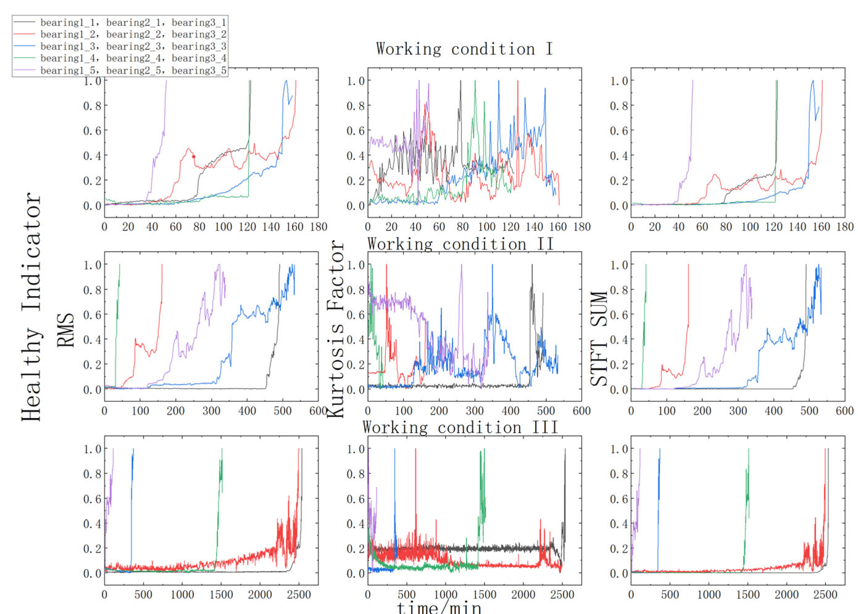
Based on the above-selected health factors, signal analysis was performed on the XJTU-SY dataset. The signal characteristics reflecting the health factors are shown in Figure 2. The RMS value starts to rise in the degradation stage and reaches the threshold value quickly in the damage stage. The kurtosis factor is suitable for the diagnosis of early failure, and the kurtosis indicator has a significant fluctuation of the trend in the health phase, which can easily misjudge the normal health phase as the fault phase. Compared with the other two health indicators, the kurtosis factor is more influenced by external noise and cannot reflect the degradation trend of bearing performance well.

2.2. Evaluation of Bearing HI

To select a reasonable health indicator, the trendability, monotonicity, and robustness are introduced to quantitatively evaluate the health indicator.

(1)

Trendability

Over time, the evolution process of bearing degradation becomes more and more serious, so the HI curve representing the development process of bearing degradation should show a certain time correlation. The characteristics of this curve are defined as a trend, and the equation is as follows:

$$\mathrm{Tre}\left(\mathrm{H},\mathrm{T}\right)=\frac{\left|{\sum }_{\mathrm{k}=1}^{\mathrm{K}}\left({\mathrm{h}}_{\mathrm{k}}- \overline{\mathrm{H}}\right)\left({\mathrm{t}}_{\mathrm{k}}-\overline{\mathrm{T}}\right)\right|}{\sqrt{{\sum }_{\mathrm{k}=1}^{\mathrm{K}}{\left({\mathrm{h}}_{\mathrm{k}}-\overline{\mathrm{H}}\right)}^2{\sum }_{\mathrm{k}=1}^{\mathrm{K}}{\left({\mathrm{t}}_{\mathrm{k}}-\overline{\mathrm{T}}\right)}^2}}$$

(1)

In Equation (1),${ \mathrm{h}}_{\mathrm{k}}$ is the sampling period HI value at ${\mathrm{t}}_{\mathrm{k}}$ time; $\overline{\mathrm{H}}=\left(1/\mathrm{K}\right){\sum }_{\mathrm{k}=1}^{\mathrm{K}}{\mathrm{h}}_{\mathrm{k}}$ is the average value of health indicators in the whole life cycle; $\overline{\mathrm{T}}=\left(1/\mathrm{K}\right){\sum }_{\mathrm{k}=1}^{\mathrm{K}}{\mathrm{t}}_{\mathrm{k}}$ is the mean value of each sampling period. $0\le \mathrm{Tre}\left(\mathrm{H},\mathrm{T}\right)\le 1$; the closer the value to 1, the better the trend.

(2)

Monotonicity

The monotonicity of the HI curve reflects the degree of degeneration of the HI curve. Although the bearing operation is in a stable stage, the bearing has also degraded over time, but the degree of degradation is weak. The monotonicity is calculated as follows:

$$\mathrm{Mon}=\left|\frac{\mathrm{num} \mathrm{of} \mathrm{dF}>0}{\mathrm{T}-1}-\frac{\mathrm{num} \mathrm{of} \mathrm{dF}<0}{\mathrm{T}-1}\right|$$

(2)

T is the number of sampling points in the bearing cycle;$\mathrm{dF}$ is the differential between the front and rear values in the HI curve.

(3)

Robustness [41]

For the characteristic signal sequence $\mathrm{F}=\left[\mathrm{f}\left(1\right),\mathrm{f}\left(2\right),\dots \mathrm{f}\left(\mathrm{K}\right)\right]$, the time sequence $\mathrm{T}=\left[\mathrm{t}\left(1\right),\mathrm{t}\left(2\right),\dots \mathrm{t}\left(\mathrm{K}\right)\right]$, $\mathrm{f}\left({\mathrm{t}}_{\mathrm{k}}\right)$ represents the characteristic value obtained at the time ${\mathrm{t}}_{\mathrm{k}}$, where $\mathrm{k}=1,2,\dots \mathrm{K}$, K represents the length of time. First, the Exponential Weighted Moving Average (EWMA) is used to divide the feature sequence into two parts, namely, the stationary trend term ${ \mathrm{f}}_{\mathrm{T}}\left({\mathrm{t}}_{\mathrm{k}}\right)$ and the random complementary vector ${\mathrm{f}}_{\mathrm{R}}\left({\mathrm{t}}_{\mathrm{k}}\right)$.

$$\mathrm{f}\left({\mathrm{t}}_{\mathrm{k}}\right)={\mathrm{f}}_{\mathrm{T}}\left({\mathrm{t}}_{\mathrm{k}}\right)+{\mathrm{f}}_{\mathrm{R}}\left({\mathrm{t}}_{\mathrm{k}}\right)$$

(3)

EWMA is calculated as follows:

$${\mathrm{f}}_{\mathrm{T}}\left({\mathrm{t}}_{\mathrm{k}}\right)={\mathsf{\beta }\mathrm{f}}_{\mathrm{T}}\left({\mathrm{t}}_{\mathrm{k}-1}\right)+\left(1-\mathsf{\beta }\right)\mathrm{f}\left({\mathrm{t}}_{\mathrm{k}}\right)$$

(4)

Equation (4) generally takes β ≥ 0.9 and ${\mathrm{f}}_{\mathrm{T}}\left({\mathrm{t}}_1\right)$ can be calculated by averaging the previous values.

Robustness is the tolerance to outliers and measures the effect of possible random fluctuations in the bearing degradation process due to random changes in sensor noise. The robustness evaluation index of F is denoted Rob(F):

$$\mathrm{Rob}\left(\mathrm{F}\right)=\frac{1}{\mathrm{K}}{\displaystyle \sum }_{\mathrm{k}}\exp \left(-\left|\frac{\mathrm{f}\left(\mathrm{k}\right)-{\mathrm{f}}_{\mathrm{T}}\left(\mathrm{k}\right)}{\mathrm{f}\left(\mathrm{k}\right)}\right|\right)$$

(5)

Based on the XJTU-SY dataset, the health indicators of 15 bearing vibration signals under 3 working conditions were evaluated respectively, and the results are shown in

Table 2. HI evaluation results.

	RMS			Kurtosis Factor			STFT SUM
	Tre	Mon	Rob	Tre	Mon	Rob	Tre	Mon	Rob
Bearing1_1	0.8632	0.6393	0.7908	0.1461	0.0328	0.7631	0.7415	0.3934	0.7613
Bearing1_2	0.9014	0.2625	0.7888	0.0595	0.1375	0.6750	0.8065	0.3500	0.7489
Bearing1_3	0.7560	0.6306	0.7775	0.7817	0.3121	0.7424	0.5804	0.5541	0.7521
Bearing1_4	0.3625	0.0083	0.7053	0.1645	0.0248	0.6589	0.2288	0.0248	0.6806
Bearing1_5	0.7584	0.4118	0.6760	0.2152	0.1373	0.8428	0.6369	0.2941	0.6728
Bearing2_1	0.3731	0.0449	0.7953	0.3905	0.0612	0.7414	0.2856	0.0082	0.7676
Bearing2_2	0.8838	0.2625	0.7798	0.1281	0.1000	0.7360	0.7200	0.2500	0.7413
Bearing2_3	0.8821	0.4812	0.8637	0.4732	0.0564	0.7555	0.8318	0.3835	0.8455
Bearing2_4	0.7909	0.7561	0.6504	0.7793	0.0244	0.6258	0.7406	0.7561	0.6414
Bearing2_5	0.9027	0.4911	0.8138	0.7806	0.1716	0.8172	0.8083	0.2840	0.7816
Bearing3_1	0.3207	0.0445	0.8944	0.1088	0.0051	0.9437	0.1934	0.0572	0.8837
Bearing3_2	0.7047	0.0790	0.8258	0.6124	0.0357	0.8545	0.5308	0.0156	0.8029
Bearing3_3	0.4141	0.2703	0.8358	0.3824	0.0649	0.7554	0.4299	0.2324	0.8232
Bearing3_4	0.3575	0.0502	0.8875	0.2468	0.1347	0.8177	0.3290	0.0568	0.8754
Bearing3_5	0.8719	0.4336	0.8320	0.2654	0.2566	0.7450	0.9046	0.4867	0.7955

. It can be seen that the calculation results of RMS indicators are good, and most parameters are higher than the kurtosis factor and STFT SUM. Therefore, the paper selected RMS as the HI of bearing health status division.

2.3. Health State Division Method

The key to the classification of bearing health status signals is to identify the fault occurrence time (FOT). The bearing signal typically goes through a stable phase, when the bearing is in the healthy stage. After FOT, the bearing degradation becomes severe and is in the fault stage.

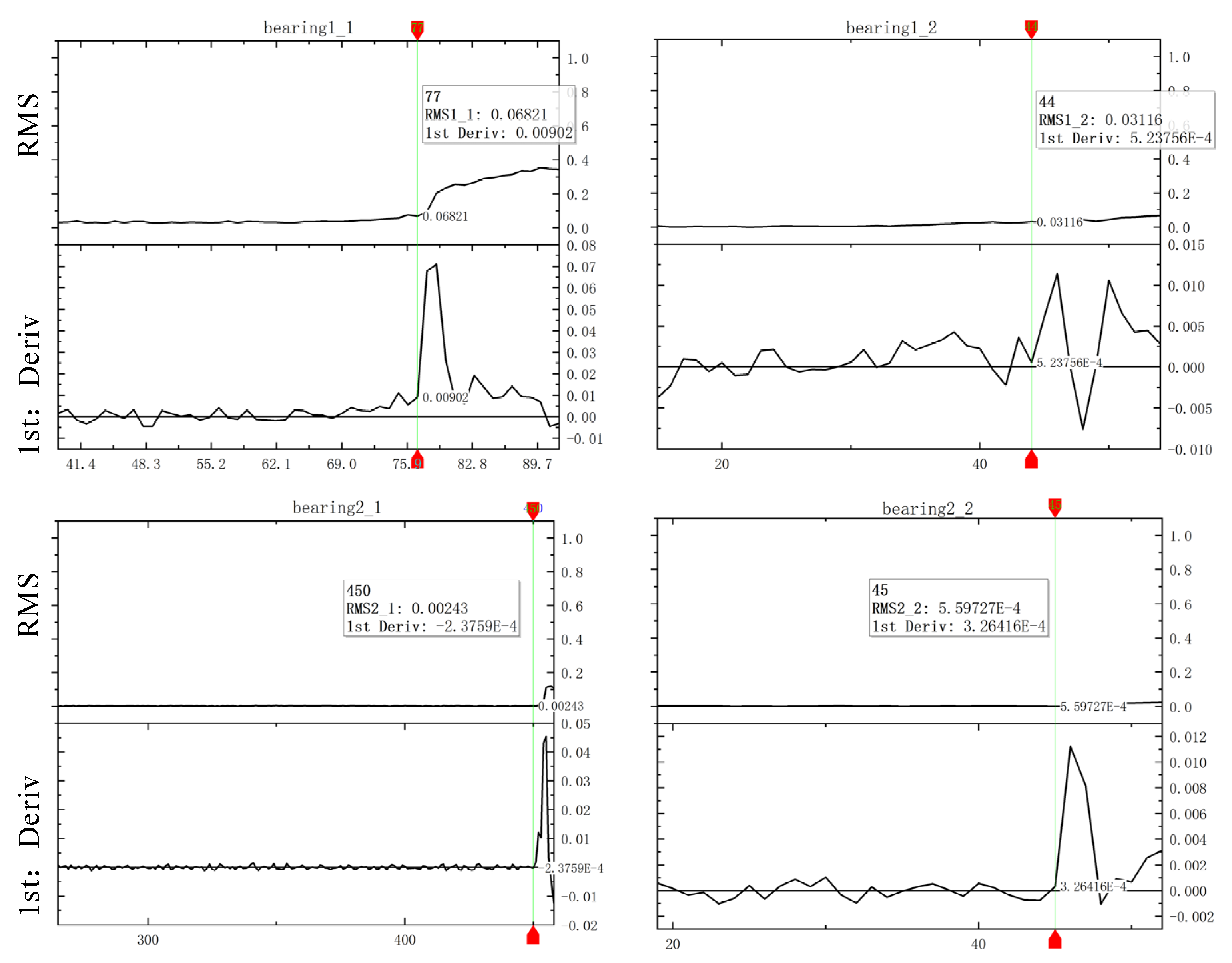
At the time of failure, the health factor will produce an elbow-point mutation due to the transition from the smooth phase to the failure phase. Therefore, in this paper, within the threshold condition of health factor 0.1, the range of abrupt change in health factor under the threshold condition is first observed to be determined. After that, the first-order differentiation of the RMS health factor within the range is performed to obtain the abrupt change condition of the RMS first-order differentiation point, to determine the health state of the bearing. The principle of bearing health state division is shown in Figure 3.

2.4. Health Status Division Results

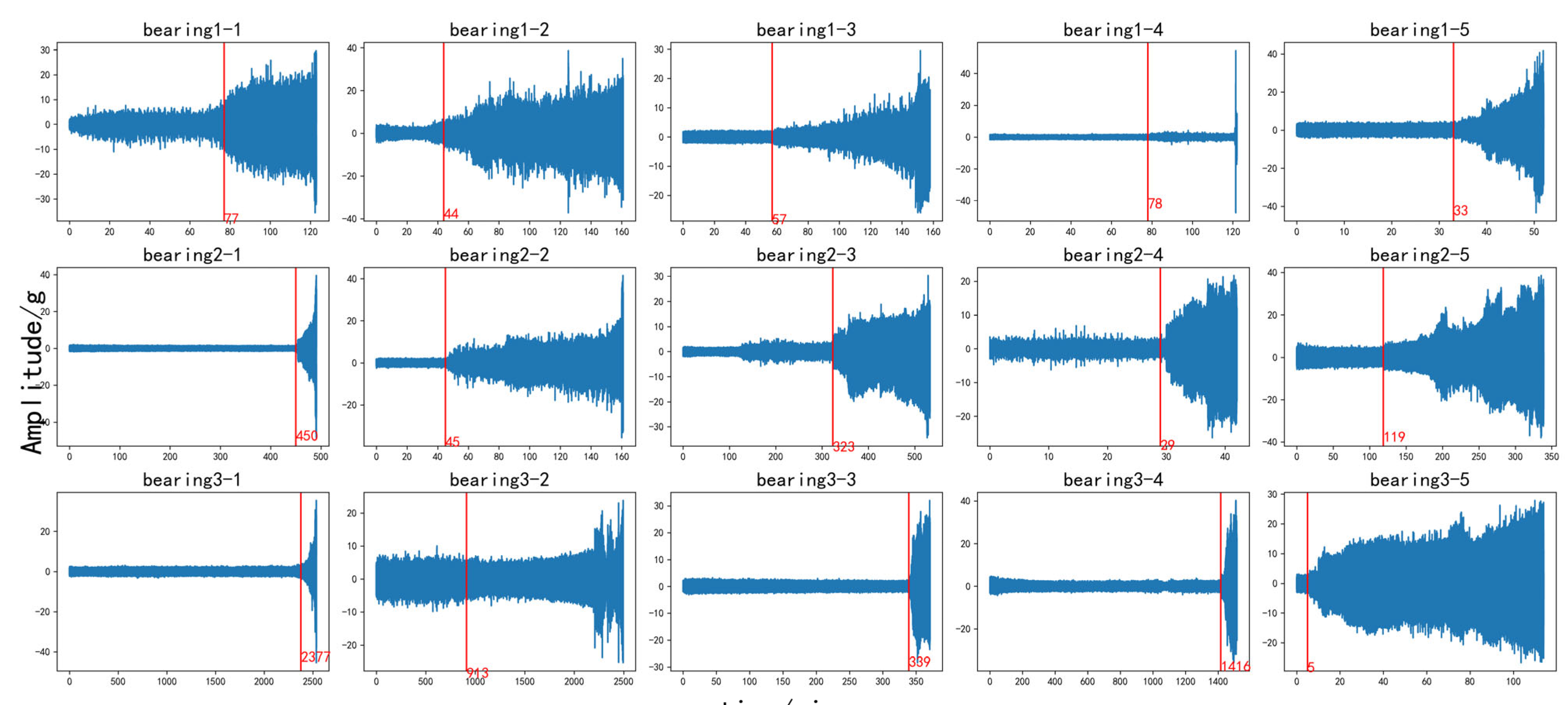
Based on the bearing vibration signal in the XJTU-SY dataset, the health status is divided, and the division results are shown in Figure 4. The long red line in the figure shows the boundary line of the healthy stage. It can be seen that the vibration signal tends to be stable in the healthy stage on the left side of the bearing vibration signal. After the failure point, the characteristic amplitude of the vibration signal shows an increasing trend with the running time, which accurately reflects the bearing degradation process.

Taking Working Condition 1 as an example, the bearing under Working Condition 1 is divided into four types of bearing states: normal, cage fault, outer-race fault, and mixed fault of inner and outer race.

Bearing normal data is the health status data before the FOT point of bearing1_1 to bearing1_5; outer ring failure data is the degradation data after the FOT point of bearing1_1 to bearing1_3; inner ring failure data is the degradation data after the FOT point of bearing1_4, and mixed inner and outer ring failure data is the degradation data after the FOT point of bearing1_5.

Since the vibration signal at the fault occurrence point is at the critical value of the fault and normal signals, and the signal points collected within 1.28 s have not been further divided, to use more reliable data, this paper discards the vibration signal at the bearing health fault occurrence point. The specific bearing health status division results of the three working conditions are shown in

Table 3. Time division of health status.

	Bearing	Bearing1_1	Bearing1_2	Bearing1_3	Bearing1_4	Bearing1_5
Fault Location
Normal		1:76	1:43	1:56	1:77	1:32
Cage					79:122
Inner-Outer-race						34:52
Outer-race		78:123	45:161	58:158
		Bearing2_1	Bearing2_2	Bearing2_3	Bearing2_4	Bearing2_5
Normal		1:449	1:44	1:322	1:28	1:118
cage				324:533
Inner-race		451:491
Outer-race			46:161		30:42	120:339
		Bearing3_1	Bearing3_2	Bearing3_3	Bearing3_4	Bearing3_5
Normal		1:2376	1:912	1:338	1:1414	1:4
Cage-Inner- outer-race			914:2496
Inner-race				340:371	1416:1515
outer-race		2378:2538				6:114

.

3. Bearing Fault Diagnosis Based on Deep Learning

In this section, according to the signal processing technology, the original signal is processed by fast Fourier transform (FFT) to extract the characteristics of the bearing vibration signal.

By building a deep learning network model, we study the bearing fault diagnosis method based on the bearing health state classification data.

3.1. FFT Feature Extraction of Time-Domain Signal

Firstly, the FFT feature of the original time-domain vibration signal is extracted, and the extracted FFT feature information is input into the neural network. The Fourier transform equation is as follows:

$$\mathrm{F}\left(\mathrm{w}\right)={{\displaystyle \int }}_{-\infty }^{\infty }\mathrm{f}\left(\mathrm{t}\right)·{\mathrm{e}}^{\mathrm{iwt}}\mathrm{dt}$$

(6)

In Equation (6), $\mathrm{F}\left(\mathrm{w}\right)$ is the Fourier transform of $\mathrm{f}\left(\mathrm{t}\right)$ and $\mathrm{w}$ is the frequency.

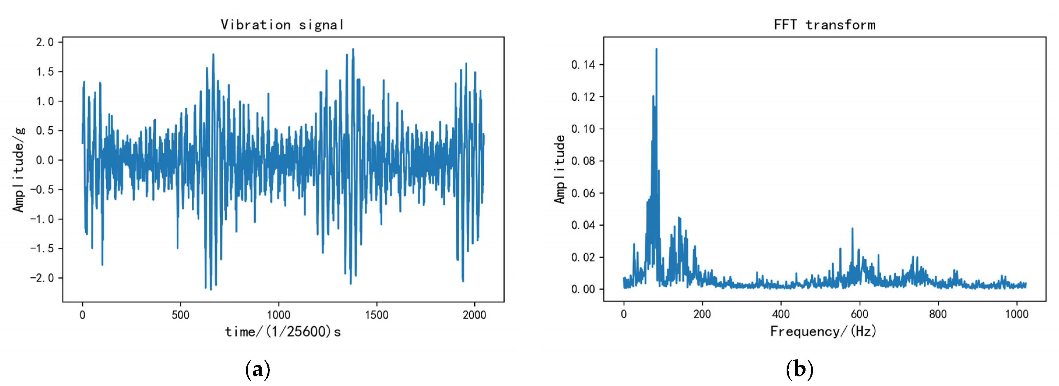
Because the frequency-domain features extracted by the Fourier transform are symmetrical, extracting the time-domain vibration signal into the frequency domain changes can reduce the amount of data by half. Because the maximum amplitude values in the frequency domain are different, the paper uniformly processes the frequency-domain signal divided by the sample length. FFT transformation of the time-domain vibration signal is shown in Figure 5.

3.2. Network Model of Bearing Fault Diagnosis Based on Deep Learning

Zhang Wei [42] of Harbin University of Technology designed a model known as “Deep Convolutional Neural Networks with Wide First layer kernel” (WDCNN) based on the characteristics of one-dimensional signal vibration.

Its structural feature is that the first layer is a wide convolution kernel. In the WDCNN network model, 64 × 1 feature extraction is used for the first layer of the large convolution kernel, and a 3 × 1 small convolution kernel and a pooling layer are used for the rest for further feature extraction.

In the WDCNN network model, the first layer of a large convolutional kernel using a single 64 × 1 convolutional kernel inevitably loses information in downsampling, so the first layer of the large convolutional kernel of different sizes is used in the original paper to verify the reliability of the model.

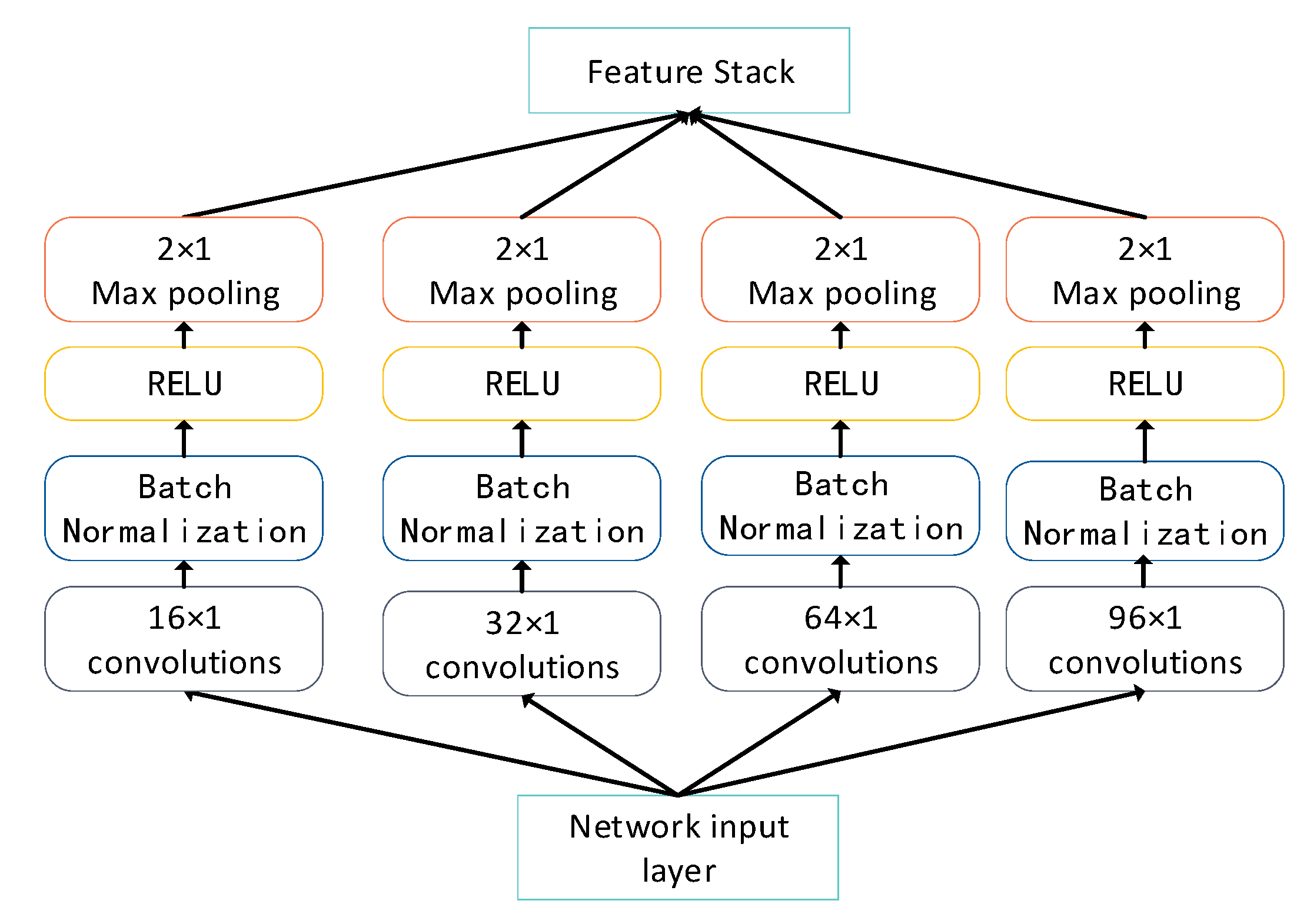
To address this feature, this paper introduces multi-scale large convolutional kernels for the first layer of large convolutional kernels based on the WDCNN model. In this paper, four different sizes of convolutional kernels, 16 × 1, 32 × 1, 64 × 1, and 96 × 1, are introduced in the first layer of a 64 × 1 large convolutional kernel to perform further feature extraction for sample information of different lengths. The structure of the first layer of the main network is shown in Figure 6.

3.3. Network Model and Detailed Parameters

The bearing vibration signal sequence has the time correlation property, and the recycle neural network has good time correlation sequence processing ability. Therefore, this paper introduces a GRU recurrent neural network to process the sequence features extracted from the convolutional layer. By combining the convolutional neural network and GRU network, the time-dependent sequences can be processed more efficiently. The utilization of the features can be improved by automatically extracting the intrinsic features of the signal using the convolutional neural network. The GRU network can then enable further processing of the features to improve the network’s ability to process time-correlated sequences. The approach combining the advantages of both neural networks can increase the ability of the network to cope with bearing fault signals in complex situations, especially strong noise situations [43].

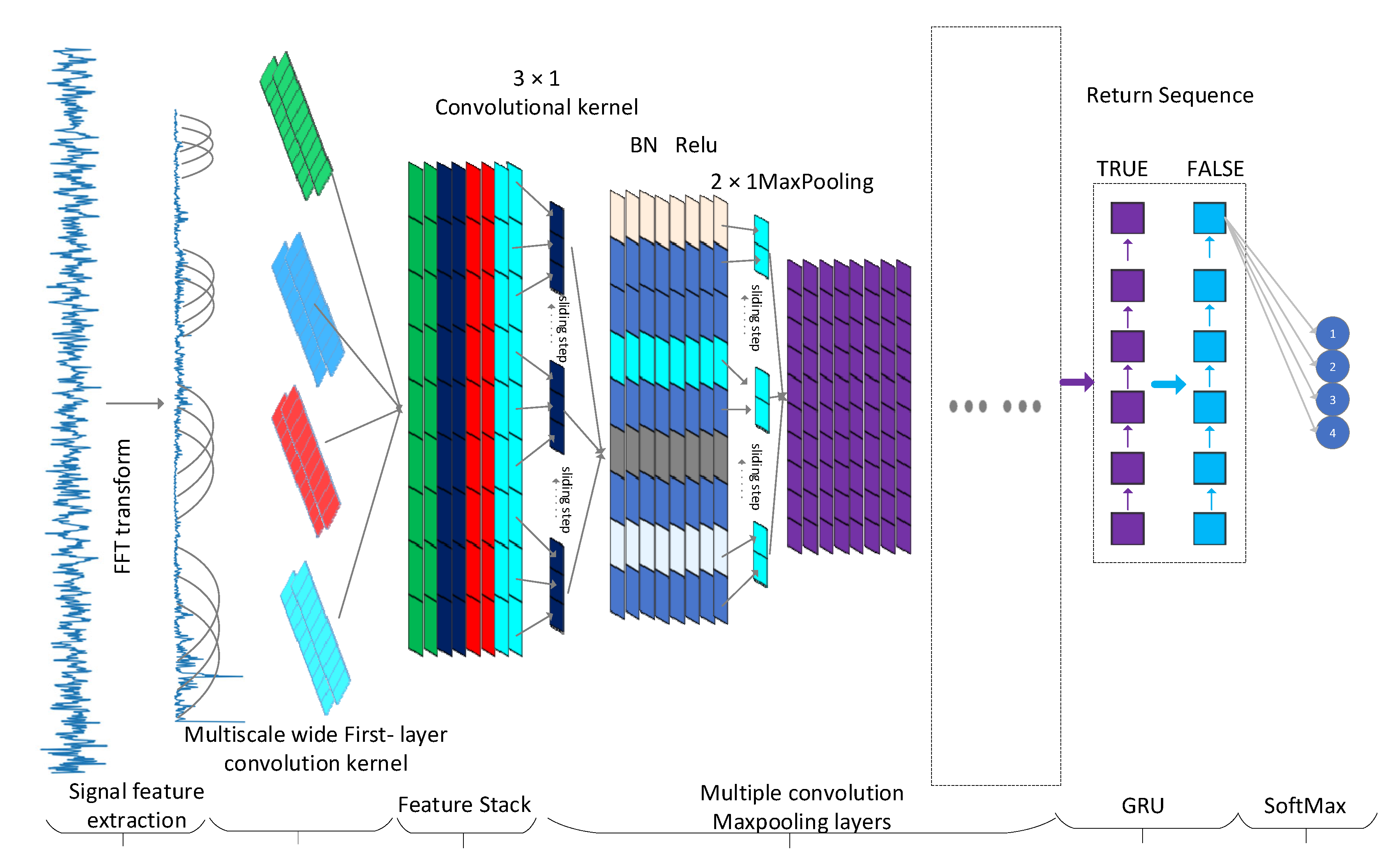
The network model proposed in this paper is shown in Figure 7. After the time-domain signal is extracted by FFT features, the first layer of the multi-scale large convolutional kernel, multi-layer 3 × 1 convolutional layer and 2 × 1 pooling layer, and GRU recurrent neural network are then used for feature extraction to further classify the rolling bearing state.

The detailed network parameters are shown in

Table 4. Detailed parameters of the network model.

NO	Layer Type	Kernel/Stride	Output Size Width × Depth		Kernel Channel Size	Padding
1	Input	—	1024 × 1		—	—
2	Convolution	16 × 1/16 × 1	64 × 8	32 × 32	8	Same
	Pooling	2 × 1/2 × 1	32 × 8		—	Valid
	Convolution	32 × 1/16 × 1	64 × 8		8	Same
	Pooling	2 × 1/2 × 1	32 × 8		—	Valid
	Convolution	64 × 1/16 × 1	64 × 8		8	Same
	Pooling	2 × 1/2 × 1	32 × 8		—	Valid
	Convolution	96 × 1/16 × 1	64 × 8		8	Same
	Pooling	2 × 1/2 × 1	32 × 8		—	Valid
3	Dropout	—	32 × 32		—	—
4	Convolution	3 × 1/1 × 1	32 × 32		32	Same
5	Pooling	2 × 1/2 × 1	16 × 32		—	Valid
6	Convolution	3 × 1/1 × 1	16 × 64		64	Same
7	Pooling	2 × 1/2 × 1	8 × 64		—	Valid
8	Convolution	3 × 1/1 × 1	8 × 64		64	Same
9	Pooling	2 × 1/2 × 1	4 × 64		—	Valid
10	Convolution	3 × 1/1 × 1	2 × 64		64	Valid
11	Pooling	2 × 1/2 × 1	1 × 64		—	Valid
12	GRU	—	1 × 60		60	—
13	GRU	—	30		30	—
14	Softmax	—	4		4	—

, with a Relu activation function layer following each convolutional layer. The purpose of introducing the activation function is to make the otherwise linear model nonlinear, allowing the model to handle linearly indistinguishable problems.

To suppress neural network overfitting, Dropout is introduced in this paper after the first large convolutional kernel and GRU layer of the multi-scale. Usually, Dropout is artificially set to 0.5 or 0.3, so the probability of lost neurons p is set to 0.3 for all Dropout layers, and the l2 regularization factor is introduced to 10⁻⁴ in each convolutional and GRU layer.

3.4. Experimental Platform and Technology

The realization of the model training in this paper adopted the Tensorflow2.2_GPU version deep learning framework based on Python3.7, and Pycharm was used for the code editing. The experimental environment was a computer with AMD R5 3500X CPU, GTX 1660s GPU, 256 G system memory, and 16 GB running memory under the Win10 system.

To improve the efficiency of the experiment and preserve the optimal model parameters of the network, Early Stopping and Save Best Only techniques are used. The Early Stopping technique ensures that the training process is terminated early when the validation accuracy no longer increases, shortening the model training time and improving the training efficiency, while the Save Best Only technique saves the model with the best performance throughout the training cycle and avoids saving the degraded model. In the experiment, the training period is set to 300 epochs, and the Early Stopping technique takes the loss function as the monitor. If the validation set loss function does not degrade for 100 consecutive epochs, the Save Best Only technique is used to save the current network model parameters. The batch_size is 256 of the original WDCNN network setting.

3.5. Experimental Process

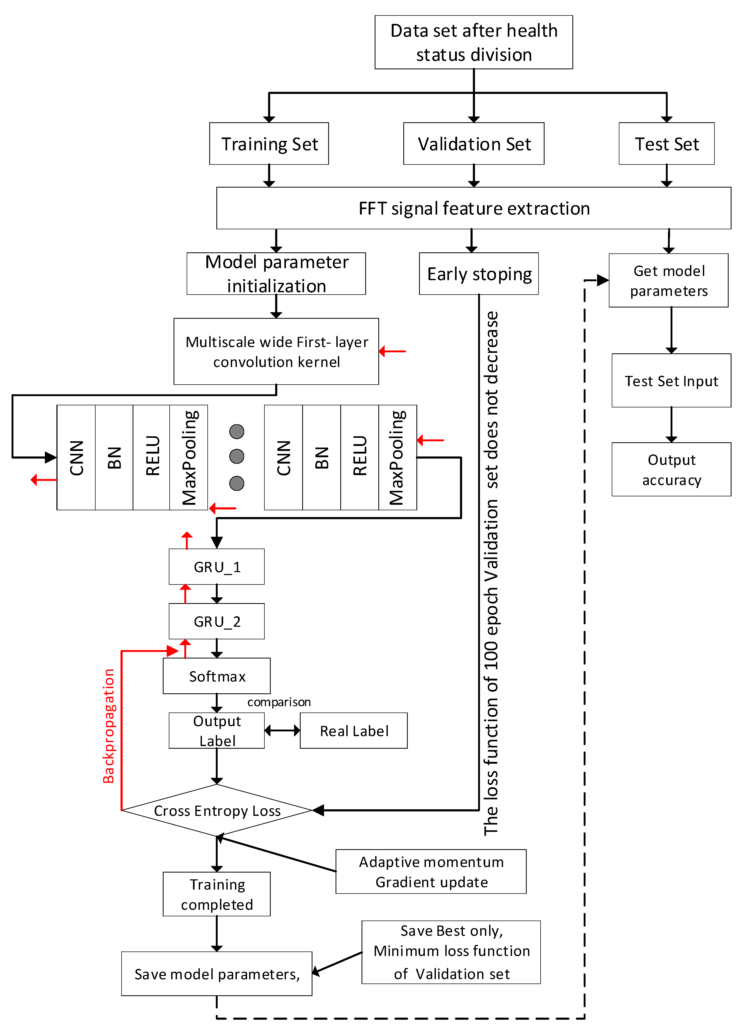
The experimental and algorithmic flow chart is shown in Figure 8. Firstly, the divided training, validation, and test datasets are pre-processed by FFT as the input of the neural network. The training set is disrupted and divided into several consecutive small batches of data (Mini Batches), each containing 256 sample data. The FFT processed training samples are then input to the neural network model, and feature extraction is performed by the first layer of the multi-scale large convolutional kernel followed by multiple small convolutional layers and pooling layers. Finally, the feature sequence information after the convolutional layer is processed by the GRU recurrent neural network, and the corresponding fault classification labels are output by the four neurons of the fully connected layer.

The model training uses a cross-entropy loss function and Adam optimizer for gradient update of output samples. The loss function of the validation set is used as the monitor, and if the loss function of the validation set does not decrease for 100 consecutive epochs, the model with the smallest loss function is used as the optimal model. After that, the test set data are input to the optimal model and the fault diagnosis classification accuracy is output.

4. Experimental Verification

4.1. Experimental Data Processing and Experimental Process Design

4.1.1. Data Enhancement

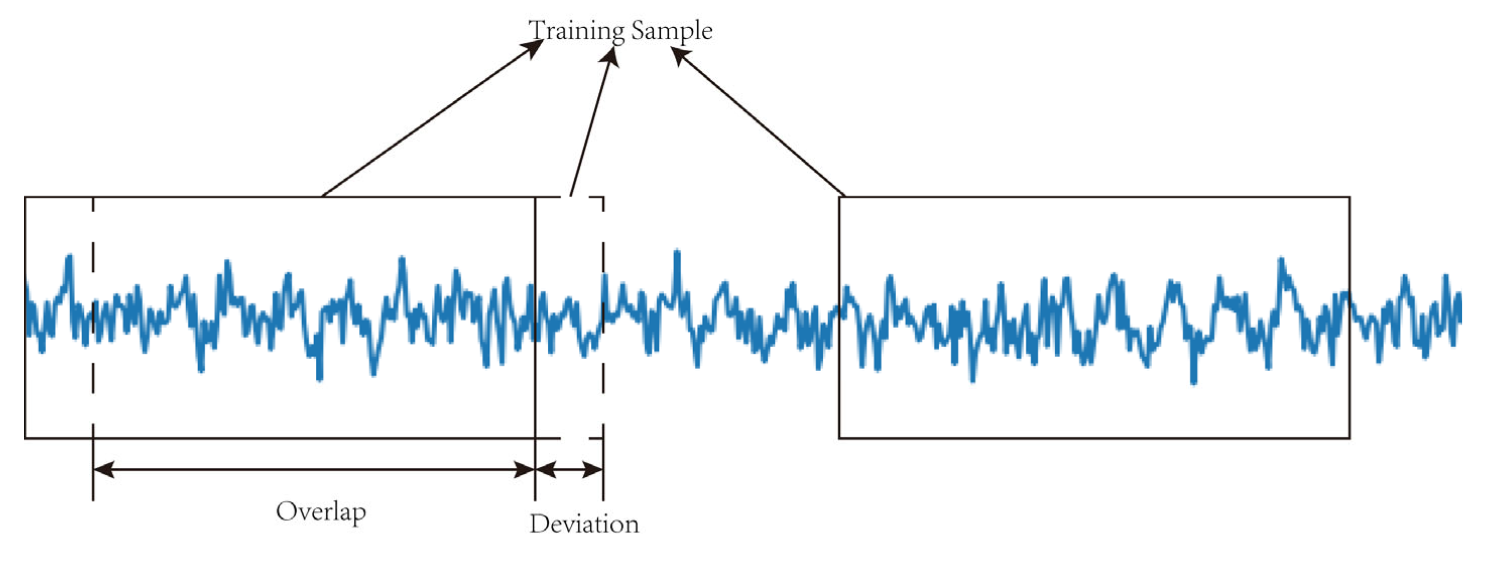
The data enhancement method proposed in this section uses the overlapping sampling method, i.e., for the training samples, each segment of the signal is acquired from the original signal with an overlap between its subsequent segments, as shown in Figure 9. For the test samples, there is no overlap in the acquisition, and the offset is set to 28 in this paper.

4.1.2. Division of Experimental Dataset

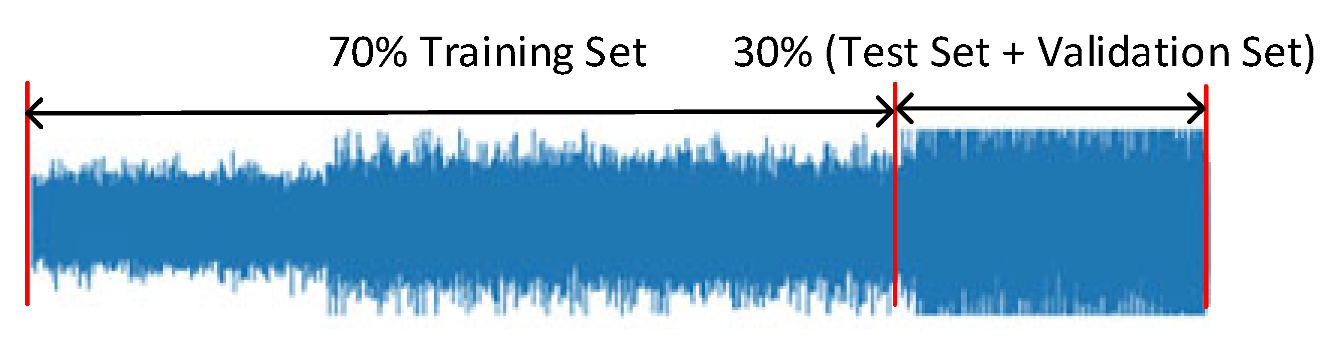
During the experiment, the first 70% of the bearing vibration signals with divided health status are set as the training set and the last 30% as the test and validation set, as shown in Figure 10.

In the whole-life degradation process of bearings, the strong degradation characteristics of the later stage of bearings are diagnosed through the early weak degradation characteristics. The different distribution of data can better reflect the generalization ability of the bearing diagnosis model. Furthermore, in the actual bearing operation process, fault diagnosis of different late health statuses is more in line with the actual operation of the bearing under health management because it can reduce unnecessary replacement maintenance costs.

In the experiments, 10,000 samples were taken for each state type in the three divided bearing datasets. The Case 1 dataset includes a total of 27,999 training data samples, 4000 validation data samples, and 8000 test data samples. Case 2 is the same as Case 1. The training set of Case 3 includes 28,000 training samples, and the data distribution of the specific division is shown in

Table 5. Description of the experimental dataset.

Working Condition I
Fault Location	Cage	Inner-Outer	Normal					Outer-Race
Type Label	0	1	2					3
Bearing	1_4	1_5	1_1	1_2	1_3	1_4	1_5	1_1	1_2	1_3
Training Set	7000	7000	1400	1400	1400	1400	1400	2333	2333	2333
Validation Set	1000	1000	200	200	200	200	200	333	333	334
Test Set	2000	2000	400	400	400	400	400	667	667	666
Working condition II
Fault location	Inner-race	Outer-race	Normal					Cage
Type Label	0	1	2					3
Bearing	2_4	2_5	2_1	2_2	2_3	2_4	2_5	2_1	2_2	2_3
Training Set	7000	7000	1400	1400	1400	1400	1400	2333	2333	2333
Validation Set	1000	1000	200	200	200	200	200	333	333	334
Test Set	2000	2000	400	400	400	400	400	667	667	666
Working condition III
Fault location	Inner-race		Normal					Outer-race		Inner-outer-cage
Type Label	0		1					2		3
bearing	3_3	3_4	3_1	3_2	3_3	3_4	3_5	3_1	3_2	3_2
Training Set	3500	3500	1400	1400	1400	1400	1400	3500	3500	7000
Validation Set	500	500	200	200	200	200	200	500	500	1000
Test Set	1000	1000	400	400	400	400	400	1000	1000	2000

.

4.2. Analysis of Experimental Results and Visualization of Training Classification Process

In this section, five sets of comparison networks are introduced to verify the feasibility of the method proposed in this paper through experimental results. The five sets of comparison network models are as follows: WDCNN + original vibration data, WDCNN + FFT signal processing, Propose + original vibration data, SVM + FFT (where SVM uses Gaussian kernel function and the error penalty term coefficient is taken as 1), and ANN + FFT (the number of neurons in each layer is 1000, 500, 300, 100, 50, and each layer uses a RELU activation function and l2 regularization). The first three sets of comparison networks are used as self-comparison experiments of the proposed network model. This paper presents a comparison with the original WDCNN network, which was the leading deep convolutional network-based bearing fault diagnosis method at that time, containing five convolutional layers and one fully connected layer. ANN and SVM are two traditional machine learning methods used for bearing fault diagnosis. ANN learns by training mechanical fault information and diagnosis experience, and then expresses the learned fault diagnosis knowledge using connection weights distributed inside the network. SVM has the advantage of solving small samples, nonlinear data, and strong generalization ability.

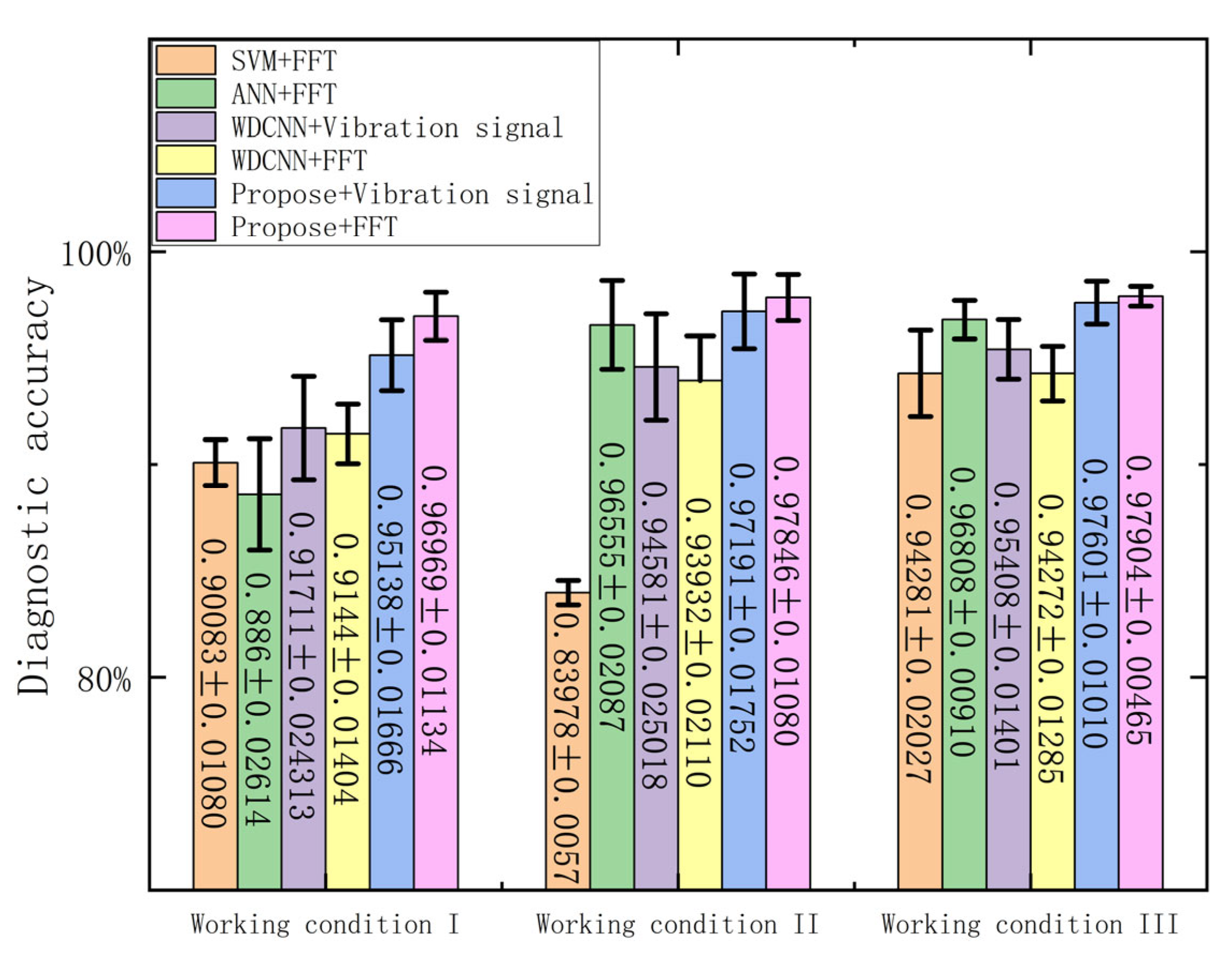
To avoid the randomness of the experiments and to ensure the credibility of the experimental comparisons, 10 repetitions of the experiments were undertaken for each model. Through the data enhancement technique, each experiment randomly grabs the divided bearing dataset under three working conditions to constitute different training sets, validation sets, and test sets to verify the reliability of the model and eliminate the influence of experimental randomness. The mean and standard deviation of the 10 experimental results were taken as the error range of the experimental results. The results are shown in Figure 11.

It can be seen from Figure 11 that the network accuracy reflected by the same network model is very different under different working condition data. FFT signal processing combined with the network model proposed in this paper (Propose + FFT) under the three working conditions obtained an average diagnostic accuracy of 96.969%, 97.846%, and 97.904% higher than other models. The standard deviation was also significantly smaller than other models, which reflects the stability of the proposed model.

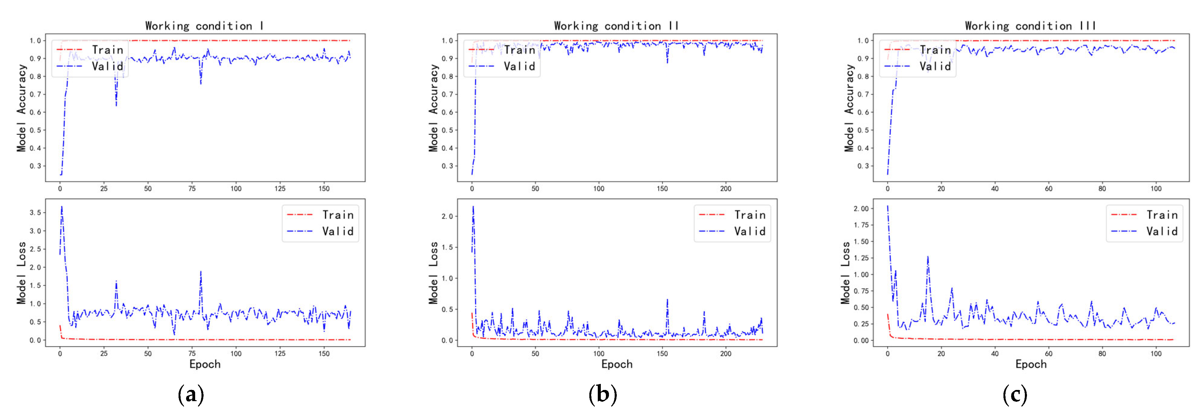
During the experiments, both the correct and loss rates of the model almost stabilized in the training set and the validation set, and the fit was good. The accuracy of the validation set was maintained at about 90%, as shown in Figure 12.

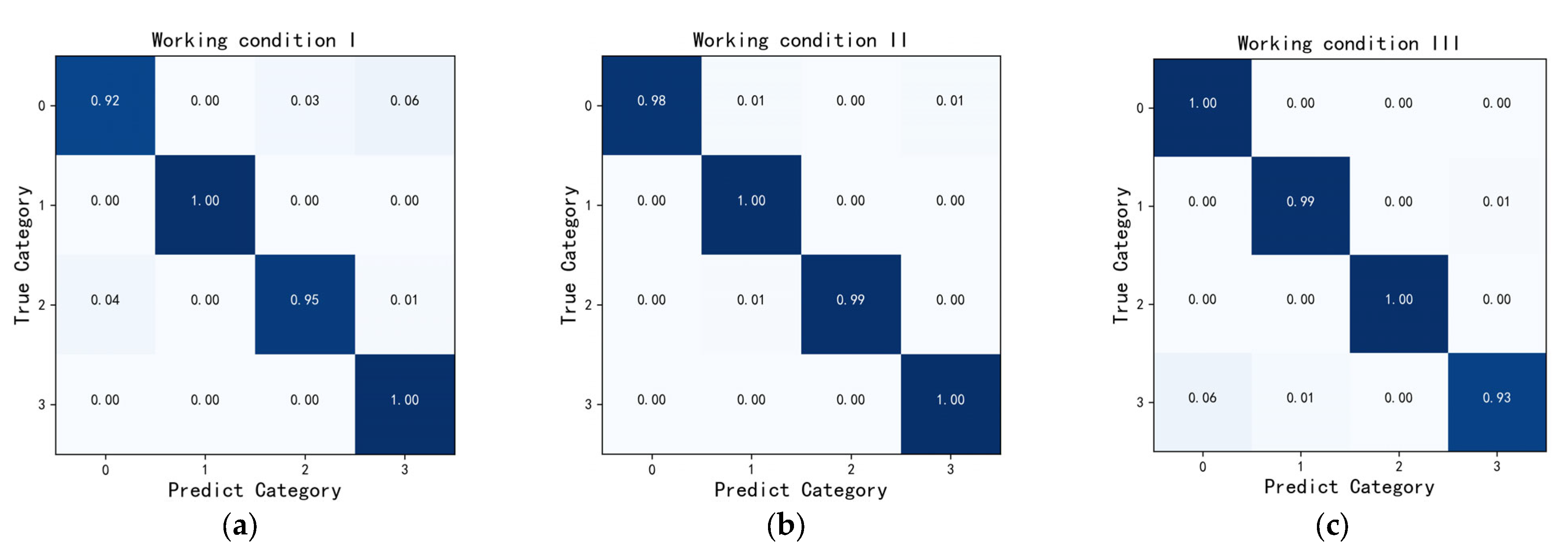
After the model training is completed, the test set is used to verify the model. The confusion matrix results are shown in Figure 13, and its values of 0, 1, 2, and 3 correspond to the fault type labels in Table 5. It can be seen that the prediction results are almost all correct. The real category 3 label of Working Condition 3 is the mixed fault of the inner and outer race rolling element, and 6% of the samples are predicted to be the inner-race fault of label 0, which is tolerable in the actual bearing fault diagnosis.

4.3. Analysis of Model Noise Resistance Results

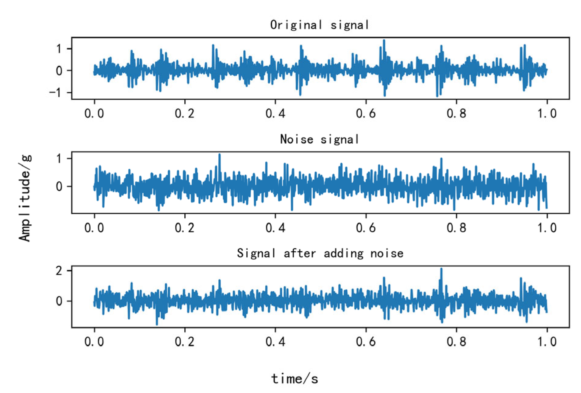
This section is designed to validate the noise immunity of the model, especially for additive Gaussian white noise, since this noise is one of the most representative noises and is easy to quantify. In this paper, the strength of the bearings subjected to industrial environmental noise is simulated by adding different signal-to-noise ratios (SNRs) [44].

The SNR is defined in Equation (7), and the unit is usually decibels (dB), where a smaller SNR indicates a more contaminated signal.

$$SN{R}_{dB}=10Lo{g}_{10}\left(\frac{P_{signal}}{P_{noise}}\right)$$

(7)

In Equation (7), $P_{signal}$ is the original signal power and $P_{noise}$ is the added noise power.

As shown in Figure 14, the original vibration signal has been completely distorted compared with the original signal after adding Gaussian white noise with SNR = 0 dB.

White Gaussian noise with a signal-to-noise ratio of −10 dB to 10 dB was added to the test set, and then the test set data were input into the saved network model. The diagnostic accuracy of the model is shown in

Table 6. Noise immunity accuracy and standard deviation range of different models.

SNR Model	−10	−8	−6	−4	−2	0	2	4	6	8	10
Working condition I
SVM + FFT ±	25.76 0.986	27.11 2.315	35.60 6.977	48.16 7.123	59.66 3.325	66.93 3.083	75.50 3.473	83.07 1.896	85.29 2.073	87.50 1.598	88.43 1.503
ANN + FFT ±	38.24 9.351	40.54 10.17	43.10 10.22	48.78 8.959	60.43 6.580	69.73 8.257	72.94 9.266	75.00 8.287	79.77 6.021	83.07 5.119	85.16 4.761
WD + Ori. ±	29.15 3.913	32.71 6.206	37.95 8.285	44.13 8.672	54.82 7.817	65.83 6.715	76.90 6.228	82.63 4.906	86.77 4.353	88.38 3.048	90.42 2.534
WD + FFT ±	30.98 6.878	32.31 6.146	35.55 7.521	40.26 9.983	49.33 11.05	60.74 10.22	71.00 8.025	80.70 6.081	84.82 5.599	87.32 3.465	88.84 1.969
Pro + Ori. ±	26.14 10.03	27.65 9.370	30.84 8.591	37.56 8.576	49.83 9.977	69.19 11.53	79.22 11.40	86.08 6.867	90.36 3.697	92.78 2.224	93.72 1.973
Pro + FFT ±	40.17 6.273	46.24 7.917	51.94 9.085	56.98 8.988	64.67 10.22	72.13 10.38	79.55 9.907	88.16 3.035	90.77 1.896	92.67 2.099	94.67 1.932
Working condition II
SVM + FFT ±	25.00 0.004	25.07 0.181	26.36 0.624	30.21 2.356	36.80 1.964	43.03 1.277	49.97 2.701	62.80 1.943	72.77 1.576	77.99 1.350	80.74 1.358
ANN + FFT ±	26.49 1.958	28.11 3.104	30.77 5.173	35.64 6.237	42.05 7.508	50.80 9.578	59.94 9.046	69.06 7.559	78.71 6.529	86.02 4.980	90.80 4.058
WD + Ori. ±	27.81 1.538	30.62 2.640	36.32 4.154	44.94 4.399	55.66 5.568	68.06 5.765	78.77 5.890	86.88 3.688	90.95 3.545	92.72 2.902	93.54 2.855
WD + FFT ±	34.74 6.813	35.99 8.284	40.02 10.43	49.55 13.88	61.59 13.86	72.25 11.21	81.22 7.872	87.05 5.154	90.07 3.787	91.69 3.061	93.12 2.472
Pro + Ori. ±	19.46 7.890	20.06 7.819	23.10 8.182	30.96 8.836	44.10 11.65	59.79 13.45	75.79 9.661	86.69 8.093	92.55 4.568	94.70 3.030	95.71 2.685
Pro + FFT ±	42.72 9.384	51.42 10.17	62.84 11.98	73.96 10.08	83.47 5.781	89.59 2.769	92.26 2.439	93.89 2.442	95.04 2.122	95.74 1.928	96.51 1.551
Working condition III
SVM + FFT ±	25.05 0.080	25.81 0.843	30.87 2.394	40.50 4.586	55.75 4.017	70.36 4.352	79.29 5.445	84.65 4.460	87.46 4.215	90.82 3.012	92.44 2.503
ANN + FFT ±	35.12 11.87	37.64 13.28	41.78 14.38	48.28 13.80	60.21 11.19	74.62 11.34	77.07 10.16	85.72 8.283	90.94 6.065	94.29 3.191	95.64 1.489
WD + Ori. ±	28.58 2.109	30.34 3.071	34.85 5.176	44.89 7.815	58.01 8.329	71.4 8.785	80.27 7.700	86.82 5.388	90.74 3.636	92.67 2.433	94.02 1.827
WD + FFT ±	27.95 5.202	28.87 65.55	30.63 6.616	33.30 6.768	40.50 7.569	55.69 7.055	67.22 7.677	77.47 6.492	82.96 4.992	87.70 3.606	90.13 2.631
Pro + Ori. ±	25.94 5.978	27.61 6.395	32.07 7.451	40.54 10.67	53.40 13.08	66.35 11.14	73.88 10.35	81.93 9.803	88.06 6.767	92.46 4.095	94.72 2.569
Pro + FFT ±	33.04 6.584	43.55 8.998	52.6 8.480	60.82 10.95	75.24 9.026	85.73 5.822	91.14 3.511	93.61 1.801	94.60 1.870	96.06 1.049	96.70 0.865

. The table shows the mean values of ten diagnostic accuracies and the range of standard deviations of ten diagnostic accuracies for different models under three working conditions.

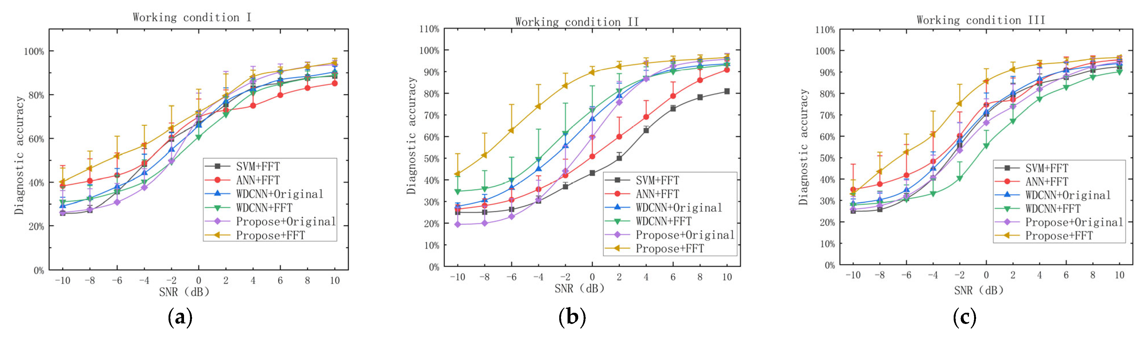
According to the data in the table, the visualization curve of the average accuracy and error range of the same model under three working conditions is constructed, as shown in Figure 15. The experimental results show that the diagnostic accuracy of the noise immunity performance of FFT signal processing combined with the proposed network (Propose + FFT) model is significantly higher than that of the other five algorithm models.

In Working Condition 1, the performance of the Propose + FFT model in the low-noise environment is not much different from that of the Propose + original vibration signal model. As the noise intensity intensifies, the diagnostic accuracy of the Propose + original vibration signal model declines sharply. In contrast, the Propose + FFT model still maintains a high diagnostic accuracy, indicating that the proposed model is also suitable for strong noise environments. The diagnostic accuracy of the ANN + FFT model is low in low-noise environments. In the environment of strong noise SNR = −10 db, although the diagnostic accuracy is higher than the other four models, it is still lower than that of the Propose + FFT model.

In Working Condition 2, the average accuracy of the Propose + FFT model is significantly higher than that of the other five models. Different from Working Condition 1 and Working Condition 3, the accuracy of the WDCNN+FFT model, except being lower than the proposed Propose + FFT algorithm, has higher diagnostic accuracy compared to the remaining four models. This indicates that the first layer of the 64 × 1 large convolutional kernel is suitable for information feature extraction in the dataset of Working Condition 2, and can extract the sample feature information more adequately. In Working Condition 2, the noise immunity performance of the Propose + original vibration signal model is the same as that in Working Condition 1. The diagnostic accuracy of the model is better in the low-noise environment, while it drops sharply in the high-noise environment. This is because the addition of low noise to the signal changes the vibration signal by a small amount, and the model can still have strong diagnostic ability. However, in a strong noise environment, the vibration signal has completely lost its original characteristics. At this time, the FFT transform is used to convert the time-domain vibration signal to the frequency-domain signal, which can ignore the time information because the frequency-domain signal can retain the original vibration information. Therefore, the FFT-transformed model can still maintain a better diagnostic classification capability in the face of strong noise. This shows the necessity of signal FFT feature extraction.

In Working Condition 3, the overall trend of various algorithms is almost the same as that of Working Condition 1. Although the ANN + FFT algorithm model retains high diagnostic accuracy even in the high-noise environment, the average diagnostic accuracy in the SNR range of −8 dB to 10 dB is still lower than that of the Propose + FFT model. In addition, the standard deviation error range of the ANN + FFT model is significantly higher than that of Propose + FFT as shown in Table 6, which also reflects the instability of the ANN + FFT model.

After the previous analysis, it can be known that the average diagnostic accuracy and error range embodied by different algorithmic models in the three operating conditions are very different, mainly due to the differences in the bearing datasets in the three operating conditions and the influence of the randomly grabbed network input sample data in the experiment. After comparison with the other five models, it can be concluded that both the average accuracy and error range of the FFT signal processing combined with the network model proposed in this paper (Propose + FFT) are better than those of the other five models under the three working conditions.

4.4. Visualization of Training Set Classification Process

In this section, the t-distributed stochastic neighbor embedding (T-SNE) technique is used to explore the classification process of small sample training data in the network model. From Table 5, it can be seen that the numbers 0 to 3 represent the types of bearing faults, respectively.

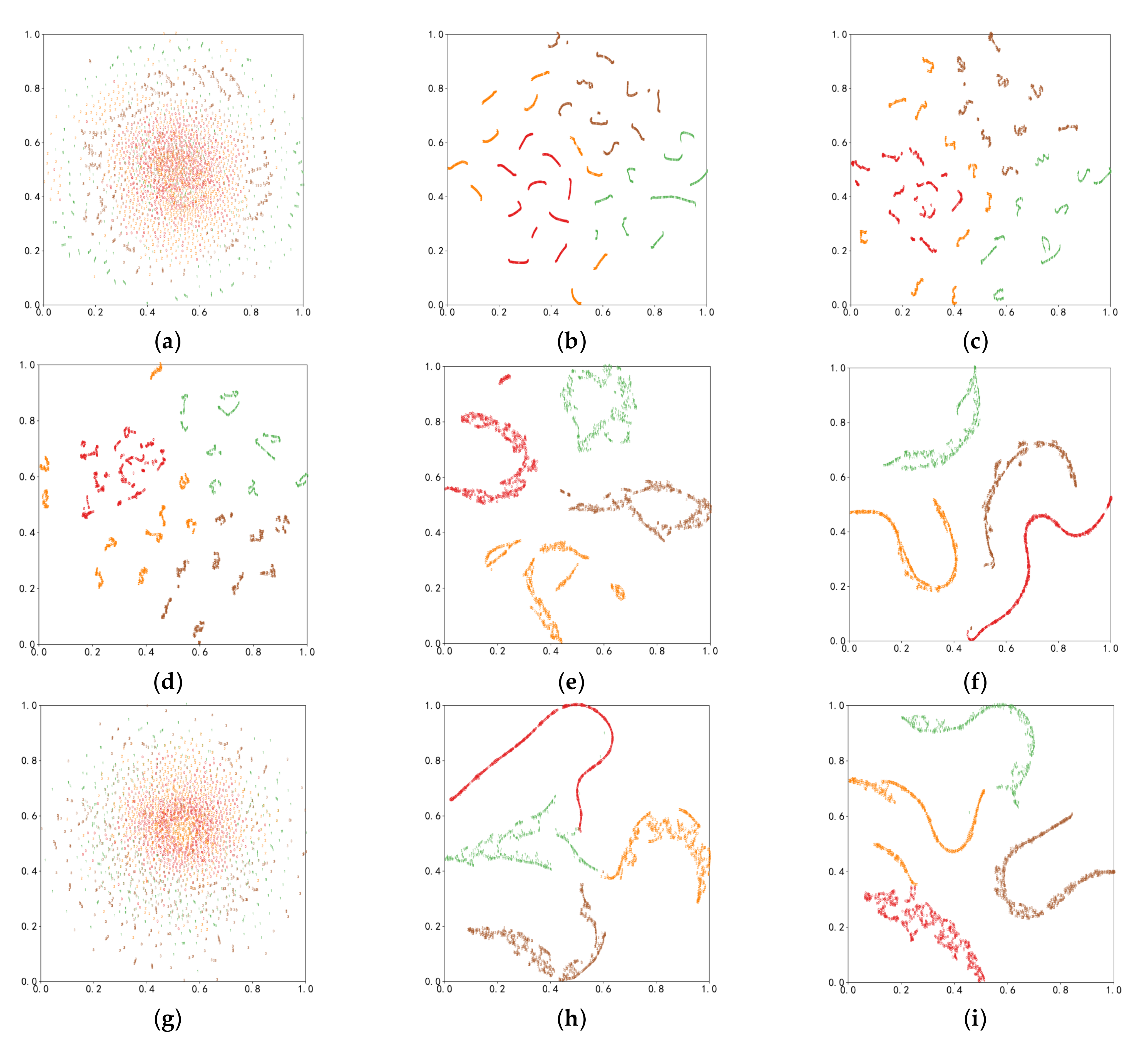
Taking the training set of Working Condition 1 as an example, one-tenth of the data volume of the training set in Table 5 is the network input data, and the T-SNE dimensionality reduction results of some network layers are shown in Figure 16.

It can be seen from Figure 16 that (1) the four health states of the bearing have been well distinguished after the FFT signal feature extraction of the training data samples, (2) the further feature extraction of the FFT data by the multi-scale first layer large convolutional kernel of the convolutional neural network and the subsequent multi-layer small convolutional kernel both further enhance the linear separability of the model for the fault features, and (3) the recurrent neural network GRU further processes the current sequence information, and the proposed network model structure improves the generalization capability of the network and the bearing fault diagnosis capability in complex situations compared with the WDCNN network.

In conclusion, the combination of FFT signal processing and the improved network model proposed in this paper has a strong ability to extract indistinguishable feature information, simplify the bearing fault diagnosis problem, and improve the bearing fault diagnosis accuracy.

4.5. Visualization of Test Set Classification Process

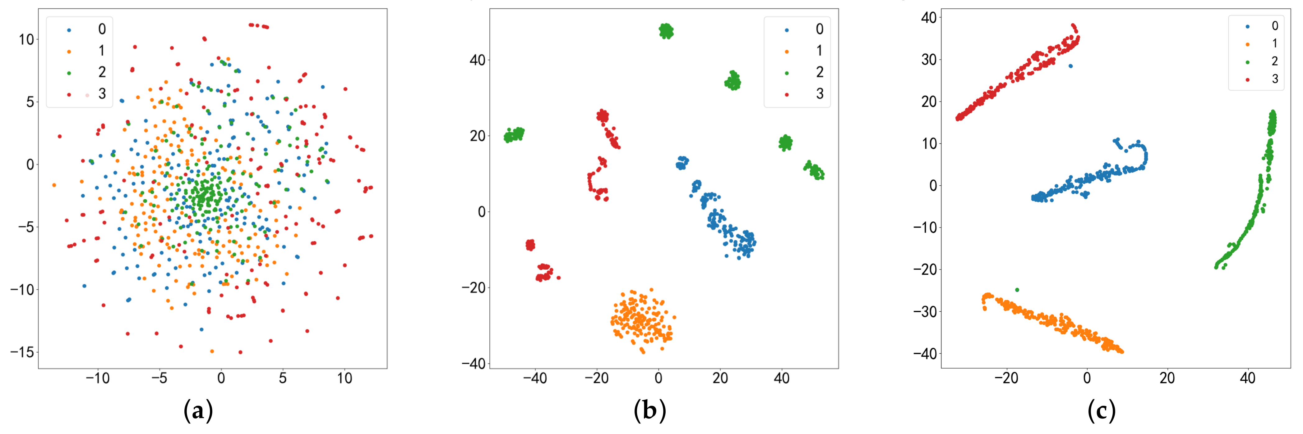
In this section, taking Working Condition 1 as an example, the features of the test set in the original data, the data after FFT signal feature extraction, and the data in the last implied layer are reduced to two dimensions and visualized respectively by the T-SNE dimensionality reduction technique, as shown in Figure 17.

It can be seen that the original vibration signal is very disorganized and it is difficult to distinguish it correctly. After FFT, the features have been clearly distinguished after using the proposed network model. The results show that the proposed network model not only has a strong classification ability in the training set, but also still maintains a strong fault diagnosis discriminative ability in the actual test.

5. Conclusions

In this paper, the vibration dataset in the field of bearing fault diagnosis research is expanded by conducting a health state classification study on the XJTU-SY bearing dataset. After that, a deep learning network model is built to classify the divided three-condition XJTU-SY dataset for fault diagnosis research. The three parameters of RMS, kurtosis, and STFT SUM are introduced to construct the bearing health factor degradation index, and quantify each health factor in terms of trend, monotonicity, and robustness. After comparison, the RMS health factor is selected, and the first-order differential mutation point under the threshold condition is used as the failure degradation starting point of the bearing, which divides the whole life cycle of the bearing into two phases: the healthy phase and the fault phase. For the divided dataset of the XJTU-SY bearing under three working conditions, based on the WDCNN algorithm, this paper establishes a deep learning network model by introducing FFT signal feature extraction, a multi-scale first-layer wide convolution kernel, and a GRU recurrent neural network.

By comparison with the other five network models (WDCNN + original vibration data, WDCNN + FFT, Propose + original vibration data, SVM + FFT, and ANN + FFT), the results show that the network model proposed in this paper has excellent fault diagnosis capability and model noise immunity, which provides important technical support for bearing fault diagnosis in actual industrial processes.

Although the proposed method has made some achievements, there are still two limitations that need to be improved in future work. Firstly, the coverage of data in this paper is not perfect and the fault diagnosis in this paper is only for historical data due to the limited practical conditions. In the future, we can build our experimental platform to collect vibration signals. Fault diagnosis can also be extended to the scope of online detection and is not limited to the application of datasets. Secondly, in this paper, when dividing the health phase and fault phase of the bearing, the division point is taken as the collected minute unit. In future work, the state within minutes will be divided step by step, and some deeper theoretical models can be applied for health state division, such as the Hidden Markov Model and the Marxian distance.

References

- Su, W. Research on Rolling Element Bearing Vibration Signal Processing and Feature Extraction Method. Ph.D. Thesis, Dalian University of Technology, Dalian, China, 2010. [Google Scholar]
- Smith, W.A.; Randall, R.B. Rolling element bearing diagnostics using the Case Western Reserve University data: A benchmark study. Mech. Syst. Signal Process. 2015, 64, 100–131. [Google Scholar]
- Nectoux, P.; Gouriveau, R.; Medjaher, K.; Ramasso, E.; Chebel-Morello, B.; Zerhouni, N.; Varnier, C. PRONOSTIA: An experimental platform for bearings accelerated degradation tests. In Proceedings of the IEEE International Conference on Prognostics and Health Management, PHM’12, Denver, CO, USA, 18–21 June 2012; pp. 1–8. [Google Scholar]
- Qiu, H.; Lee, J.; Lin, J.; Yu, G. Wavelet filter-based weak signature detection method and its application on rolling element bearing prognostics. J. Sound Vib. 2006, 289, 1066–1090. [Google Scholar] [CrossRef]
- Yaguo, L.; Tianyu, H.; Biao, W.; Naipeng, L.; Tao, Y.; Jun, Y. XJTU-SY Rolling Element Bearing Accelerated Life Test Datasets: A Tutorial. J. Mech. Eng. 2019, 55, 1–6. [Google Scholar] [CrossRef]
- Wang, B.; Lei, Y.; Li, N.; Li, N. A hybrid prognostics approach for estimating remaining useful life of rolling element bearings. IEEE Trans. Reliab. 2018, 69, 401–412. [Google Scholar] [CrossRef]
- Wang, B.; Lei, Y.; Li, N.; Wang, W. Multiscale convolutional attention network for predicting remaining useful life of machinery. IEEE Trans. Ind. Electron. 2020, 68, 7496–7504. [Google Scholar] [CrossRef]
- Wang, B.; Lei, Y.; Li, N.; Yan, T. Deep separable convolutional network for remaining useful life prediction of machinery. Mech. Syst. Signal Process. 2019, 134, 106330. [Google Scholar] [CrossRef]
- Wang, B.; Lei, Y.; Yan, T.; Li, N.; Guo, L. Recurrent convolutional neural network: A new framework for remaining useful life prediction of machinery. Neurocomputing 2020, 379, 117–129. [Google Scholar] [CrossRef]
- Kim, D.W.; Lee, E.S.; Jang, W.K.; Kim, B.H.; Seo, Y.H. Effect of data preprocessing methods and hyperparameters on accuracy of ball bearing fault detection based on deep learning. Adv. Mech. Eng. 2022, 14, 16878132221078494. [Google Scholar] [CrossRef]
- Zhong, H.; Lv, Y.; Yuan, R.; Yang, D. Bearing fault diagnosis using transfer learning and self-attention ensemble lightweight convolutional neural network. Neurocomputing 2022, 501, 765–777. [Google Scholar] [CrossRef]
- Pandya, D.H.; Upadhyay, S.H.; Harsha, S.P. ANN Based Fault Diagnosis of Rolling Element Bearing Using Time-Frequency Domain Feature. Int. J. Eng. Sci. Technol. 2012, 4, 2878–2886. [Google Scholar]
- Xin, W.; Wenyuan, Y. Fault diagnosis of rolling bearings based on variational modal decomposition and SVM. J. Vib. Shock 2017, 36, 252–256. [Google Scholar]
- Hinton, G.E.; Salakhutdinov, R.R. Reducing the Dimensionality of Data with Neural Networks. Science 2006, 313, 504–507. [Google Scholar] [CrossRef] [Green Version]
- Ghaderzadeh, M.; Aria, M.; Hosseini, A.; Asadi, F.; Bashash, D.; Abolghasemi, H. A Fast and Efficient CNN Model for B-ALL Diagnosis and Its Subtypes Classification Using Peripheral Blood Smear Images. Int. J. Intell. Syst. 2022, 37, 5113–5133. [Google Scholar] [CrossRef]
- Ghaderzadeh, M.; Asadi, F.; Jafari, R.; Bashash, D.; Abolghasemi, H.; Aria, M. Deep Convolutional Neural Network–Based Computer-Aided Detection System for COVID-19 Using Multiple Lung Scans: Design and Implementation Study. J. Med. Internet Res. 2021, 23, e27468. [Google Scholar] [CrossRef]
- Gheisari, M.; Ebrahimzadeh, F.; Rahimi, M.; Moazzamigodarzi, M.; Liu, Y.; Dutta Pramanik, P.K.; Heravi, M.A.; Mehbodniya, A.; Ghaderzadeh, M.; Feylizadeh, M.R.; et al. Deep Learning: Applications, Architectures, Models, Tools, and Frameworks: A Comprehensive Survey. CAAI Trans Intell. Technol. 2023, cit2.12180. [Google Scholar] [CrossRef]
- Garavand, A.; Salehnasab, C.; Behmanesh, A.; Aslani, N.; Zadeh, A.H.; Ghaderzadeh, M. Efficient Model for Coronary Artery Disease Diagnosis: A Comparative Study of Several Machine Learning Algorithms. J. Healthc. Eng. 2022, 2022, 5359540. [Google Scholar] [CrossRef]
- Ghaderzadeh, M.; Aria, M. Management of Covid-19 Detection Using Artificial Intelligence in 2020 Pandemic. In Proceedings of the 2021 5th International Conference on Medical and Health Informatics, Kyoto, Japan, 14 May 2021; ACM: New York, NY, USA, 2021; pp. 32–38. [Google Scholar]
- Krizhevsky, A.; Sutskever, I.; Hinton, G.E. Imagenet classification with deep convolutional neural networks. Commun. ACM 2017, 60, 84–90. [Google Scholar] [CrossRef] [Green Version]
- Srivastava, N.; Hinton, G.; Krizhevsky, A.; Sutskever, I.; Salakhutdinov, R. Dropout: A simple way to prevent neural networks from overfitting. J. Mach. Learn. Res. 2014, 15, 1929–1958. [Google Scholar]
- Szegedy, C.; Liu, W.; Jia, Y.; Sermanet, P.; Reed, S.; Anguelov, D.; Erhan, D.; Vanhoucke, V.; Rabinovich, A. Going deeper with convolutions. In Proceedings of the IEEE Conference on Computer Vision and Pattern Recognition, Boston, MA, USA, 7–12 June 2015; pp. 1–9. [Google Scholar]
- He, K.; Zhang, X.; Ren, S.; Sun, J. Deep residual learning for image recognition. In Proceedings of the IEEE Conference on Computer Vision and Pattern Recognition, Las Vegas, NV, USA, 26 June–1 July 2016; pp. 770–778. [Google Scholar]
- Graves, A. Long Short-Term Memory. In Supervised Sequence Labeling with Recurrent Neural Networks; Springer: Berlin&Heidelberg, Germany, 2012; Volume 385, pp. 37–45. [Google Scholar]
- Cho, K.; Van Merriënboer, B.; Gulcehre, C.; Bahdanau, D.; Bougares, F.; Schwenk, H.; Bengio, Y. Learning phrase representations using RNN encoder-decoder for statistical machine translation. arXiv 2014, arXiv:1406.1078 2014. [Google Scholar]
- Xie, W.; Li, Z.; Xu, Y.; Gardoni, P.; Li, W. Evaluation of Different Bearing Fault Classifiers in Utilizing CNN Feature Extraction Ability. Sensors 2022, 22, 3314. [Google Scholar] [CrossRef]
- Xia, Y.; Shen, C.; Wang, D.; Shen, Y.; Huang, W.; Zhu, Z. Moment matching-based intraclass multisource domain adaptation network for bearing fault diagnosis. Mech. Syst. Signal Process. 2022, 168, 108697. [Google Scholar] [CrossRef]
- Wang, R.; Jiang, H.; Zhu, K.; Wang, Y.; Liu, C. A deep feature enhanced reinforcement learning method for rolling bearing fault diagnosis. Adv. Eng. Inform. 2022, 54, 101750. [Google Scholar] [CrossRef]
- Li, J.; Liu, Y.; Li, Q. Intelligent fault diagnosis of rolling bearings under imbalanced data conditions using attention-based deep learning method. Measurement 2022, 189, 110500. [Google Scholar]
- Zhang, J.; Sun, Y.; Guo, L.; Gao, H.; Hong, X.; Song, H. A New Bearing Fault Diagnosis Method Based on Modified Convolutional Neural Networks. Chin. J. Aeronaut. 2020, 33, 439–447. [Google Scholar] [CrossRef]
- Li, Z.; Li, Y.; Sun, Q.; Qi, B. Bearing Fault Diagnosis Method Based on Convolutional Neural Network and Knowledge Graph. Entropy 2022, 24, 1589. [Google Scholar] [CrossRef] [PubMed]
- Xu, G.; Liu, M.; Jiang, Z.; Söffker, D.; Shen, W. Bearing Fault Diagnosis Method Based on Deep Convolutional Neural Network and Random Forest Ensemble Learning. Sensors 2019, 19, 1088. [Google Scholar] [CrossRef] [Green Version]
- Zhang, J.; Kong, X.; Li, X.; Hu, Z.; Cheng, L.; Yu, M. Fault Diagnosis of Bearings Based on Deep Separable Convolutional Neural Network and Spatial Dropout. Chin. J. Aeronaut. 2022, 35, 301–312. [Google Scholar] [CrossRef]
- Wei, X. Deep Learning Based Health State Assessment And Remaining Life Prediction of Rolling Bearings. Master’s Thesis, Southwest Jiaotong University, Chengdu, China, 2021. [Google Scholar]
- Lin, F. Research on Construction Method of HI Curve in Bearing Life. Master’s Thesis, North China Electric Power University, Baoding, China, 2021. [Google Scholar]
- Yin, A.; Liang, Z.; Zhang, B.; Wang, D. Evaluation Method of Bearing Health State Based on Similarity of Principal Curve. J. Vib. Meas. Diagn. 2019, 39, 625–630+676. [Google Scholar]
- Yin, A.; Wang, Y.; Dai, Z.; Ren, H. Evaluation Method of Bearing Health State Based on Variation Auto-Encoder. J. Vib. Meas. Diagn. 2020, 40, 1011–1016. [Google Scholar]
- Ke, Y. Performance Degradation Stage Division and Remaining Useful Life Prediction of Rolling Bearing Based on Multi-Domain Features. Master’s Thesis, Lanzhou University of Technology, Lanzhou, China, 2021. [Google Scholar]
- Zhu, J.; Chen, N.; Shen, C. A new data-driven transferable remaining useful life prediction approach for bearing under different working conditions. Mech. Syst. Signal Process. 2020, 139, 106602. [Google Scholar]
- Satopaa, V.; Albrecht, J.; Irwin, D.; Raghavan, B. Finding a “kneedle” in a haystack: Detecting knee points in system behavior. In Proceedings of the 2011 31st International Conference on Distributed Computing Systems Workshops, Minneapolis, MI, USA, 20–24 June 2011; pp. 166–171. [Google Scholar]
- Liu, S.-L.; Gao, L.-H.; Du, J.-W.; Liu, C. Rolling bearing remaining useful life prediction via adaptive sequential optimal feature. Ship Sci. Technol. 2019, 41, 71–76. [Google Scholar]
- Zhang, W. Study on Bearing Fault Diagnosis Algorithm Based on Convolutional Neural Network. Master’s Thesis, Harbin Institute of Technology, Harbin, China, 2017. [Google Scholar]
- Jin, G. Research on End-to-End Bearing Fault Diagnosis Based on Deep Learning Under Complex Conditions. Ph.D. Thesis, University of Science and Technology of China, Hefei, China, 2020. [Google Scholar]
- Jin, G.; Li, D.; Wei, Y.; Hou, W.; Jin, Y. Bearing fault diagnosis using structure optimized deep convolutional neural network under noisy environment. IOP Conf. Ser. Mater. Sci. Eng. 2019, 630, 012018. [Google Scholar] [CrossRef] [Green Version]
Figure 1.
Experimental platform (provided by the XJTU-SY dataset [5]).
Figure 2.
Signal analysis of bearing HI.
Figure 3.
Signal division of bearing health status.
Figure 4.
Result of bearing health status division.
Figure 5.
FFT of bearing vibration signal: (a) Vibration signal; (b) FFT transform.
Figure 6.
Multi-scale first-layer wide convolution kernel.
Figure 7.
Structure of the network model.