Article

Experimental Simulation of Thunderstorm Profiles in an Atmospheric Boundary Layer Wind Tunnel

by
Camila Aldereguía Sánchez
1,2,
Federica Tubino
1,
Anna Bagnara
3 and
Giuseppe Piccardo
1,*
1
Department of Civil, Chemical and Environmental Engineering, University of Genoa, 16145 Genoa, Italy
2
Faculty of Civil Engineering, Technological University of Havana José Antonio Echeverría CUJAE, La Habana 19390, Cuba
3
NOVA Fluid Mechanics, Teddington TW11 8EZ, UK
*
Author to whom correspondence should be addressed.
Submission received: 21 March 2023 / Revised: 1 July 2023 / Accepted: 4 July 2023 / Published: 10 July 2023
(This article belongs to the Special Issue Structural Wind Engineering)

Abstract

:
Thunderstorms have different features in comparison with synoptic events, including a typical nose-shaped mean wind speed profile and non-stationary characteristics in time intervals from 10 min to 1 h. The simulation of thunderstorms in traditional wind tunnels requires suitable devices in order to replicate their peculiar characteristics. Disregarding the non-stationary characteristics of thunderstorm outflows, this paper aims to study the possibility of adopting a passive device such as a specially designed grid in order to reproduce the nose-shaped mean wind speed profile. A widely adopted model of the mean wind velocity profile from the literature is employed as a target profile for the verification of the experimental findings. The results obtained show a good agreement between the measured and target mean wind speed profiles and an acceptable turbulence intensity level compared with full-scale and experimental measurements. The proposed device offers a practical and cost-effective solution to simulate the main characteristics of a thunderstorm event in a traditional atmospheric boundary layer wind tunnel, which could be adopted to assess the significance of thunderstorm loading on civil engineering structures and define the requirement for ad hoc specialist studies.

1. Introduction

Thunderstorm (TS) is a weather phenomenon characterized by an intense form of convection that in some cases would produce a downburst. The wind velocity associated with downbursts is non-stationary in time intervals of 10 min to 1 h, and the vertical profile of the slowly varying mean component has a characteristic nose-shape [1]. In particular, the maximum wind velocities (i.e., the nose) tend to occur at heights of around 50 m to 120 m [2]; however, there are uncertainties regarding the parameters that govern the height of the nose. In some cases, wind speeds due to thunderstorms are comparable in magnitude to those of strong synoptic events, leading to the collapse of many structures around the world, especially low-rise structures such as transmission towers, harbor cranes, warehouses, signboards and canopies, which are currently being designed for standard synoptic events. This may be due to the fact that, typically, in structural design, reference wind velocities evaluated from databases and codes of practice containing synoptic and thunderstorm events are considered in conjunction with standard boundary layer wind speed profiles. For low-rise structures this approach could give rise to unsafe designs, due to the coincidence of their average heights with the height of the nose [3]. For tall buildings, this methodology is most likely conservative, since assuming a typical logarithmic mean wind profile could provide an overestimate of wind actions with respect to downburst profiles, characterized by a maximum velocity at intermediate heights above the ground. The effect of thunderstorm downbursts on civil engineering structures has become a focus of several investigations and studies around the world with the ultimate goal of codifying methodologies that would allow designers to safely design structures against these events. Despite the effort in the study of these phenomena, a comprehensive analytical model for thunderstorm outflows and their loading on structures, similar to that provided for synoptic events, is still not available [4].
Analytical models for the mean wind speed profile have been developed through the analysis of field measurements, laboratory tests and numerical simulations. The key parameters in the vertical profile representation are the height of the nose and the maximum velocity at this height. A literature review of several research studies [2,5,6] indicates that the maximum horizontal velocity appears in the interval 50–120 m above ground level. In terms of turbulence intensity, a consolidated model to recreate the vertical profile is not available due to the shortage of multi-point full-scale measurements for these phenomena. Therefore, some papers in the literature propose a constant value of turbulence intensity independent on the height (e.g., [7]).
Wind tunnel testing is an effective tool to estimate wind loading, especially on tall buildings [8,9]. Experimental simulation of thunderstorm downbursts can be carried out in two types of facilities: 3D wind simulators and Atmospheric Boundary Layer (ABL) wind tunnels. The most widespread technique aimed to reproduce downburst is the impinging wall jet, in which a jet impinges on a flat surface to create a wall radial outflow and a vortex ring, using equipment built for this specific purpose (e.g., [8,10]). However, these types of facilities are expensive and normally available in research centers, where standard civil engineering projects do not have an easy access to them. Therefore, more practical and cost-effective approaches have been proposed in order to reproduce thunderstorm outflow conditions in ABL wind tunnels. Investigations have been developed to reproduce downburst outflow in traditional wind tunnels, using active devices such as multi-blade flow systems (e.g., [11,12]) or in a new generation of facilities such as multiple-fan wind tunnels (e.g., [13,14]). These techniques can simulate both the nose-shaped profile, and some non-stationary characteristics of thunderstorm downbursts.
The objective of this paper is to propose the use of a passive device to reproduce the wind speed profile of thunderstorm downbursts in an ABL wind tunnel. For this purpose, a specially designed grid was used in addition to traditional devices in order to replicate thunderstorm mean wind speed and turbulence profiles, hence avoiding active devices. The temporal evolution of the thunderstorm is not considered, and attention is focused only on the vertical mean wind speed profile corresponding to the worst-case scenario with respect to the structural response (i.e., during the velocity ramp-up, at the end of the passage of the primary vortex, e.g., [10]). This study represents the first stage of a research project aimed at comparing wind loads and cladding pressures generated on tall buildings of heights in the range of 100 m to 300 m, by synoptic and thunderstorm phenomena.
At first, a literature review about the available experimental techniques for thunderstorm downburst simulation and their properties in terms of mean profile and turbulence characteristics is provided in Section 2. Then, Section 3 presents the experimental setup adopted. The results and main observations during the tests are discussed in Section 4, in terms of mean velocity and turbulence properties. Finally, the conclusions of the work are given in Section 5.

2. Literature Review

2.1. Experimental Simulation of Thunderstorm Downbursts

The temperature and relative humidity variations at different levels play a crucial role in the development of downbursts [15]. However, climatic wind tunnels, despite their capability to control temperature and relative humidity, generally do not replicate the key aspects that are most relevant to structural loading, such as the mean velocity and longitudinal turbulence profiles. Consequently, when it comes to structural applications in the field of wind engineering, the experimental simulation of downbursts is typically constrained to reproducing the velocity field generated by these events. The simulation of the velocity field associated with downbursts can be carried out in two groups of facilities. The first group can simulate the entire downburst event, reproducing the spatial and temporal variation of the associated wind field, while the second one is only able to replicate the main characteristics of outflows. Facilities from the first group can be called 3D wind simulators due to their unique capabilities of reconstructing the entire downburst event, creating a wall radial outflow and a vortex ring with the impinging jet technique. In these facilities, different experimental simulations have been carried out: isolated downdraft, i.e., stationary downburst without background flow [8,16], translational downdraft [17,18] and both cases embedded into ABL-like winds [19]. This type of experimental test requires the same length scale for the simulated downburst and the structure; thus, large facilities are needed, which makes them expensive and consequently not very common. Moreover, for the reasons specified, the scale of the structural model is usually very small (e.g., [20]). Therefore, this type of test is essentially carried out in research centers, and regular civil projects do not have easy access to them.
Due to these issues, researchers have been focused on developing alternatives to recreate the main features of downburst outflows in the most common facilities, i.e., ABL Wind Tunnels. Therein, the downdraft phenomenon is not fully simulated: suitable devices are adopted in order to reproduce the downburst gust front. In single-fan wind tunnels, this type of simulation is based on redirecting the horizontal flow; thus, the facility has to be equipped with specific active devices, such as single- or multi-blade systems. Regarding the first case, Butler and Kareem [21] carried out an experimental test using a manually controlled pivoted flat plate. Concerning the latter case, Le and Caracoglia [12] simulated the downburst outflows in a small-scale ABL wind tunnel proposing a simplified multi-blade flow device. Aboutabikh et al. [11] suggested and calibrated in three stages a system of multiple louvers using numerical simulations. In this context, a downburst simulator was developed at the multiple-fan Wall of Wind (WoW) laboratory of Florida International University, consisting of two louvers located near the ground, able to simulate the gust front [22,23], which was later used on an aeroelastic model by Alawode et al. [24] to evaluate its dynamic response. In the case of multiple-fan wind tunnels built with small (or very small) fans, in order to favor their time response without using any kind of blade system, the ability to control the performance of each of the different fans allows the generation of target wind speed time histories and profiles. Therefore, these new-generation facilities are, by their nature, capable of simulating the impact of two distinct features of gust front flows: the near-ground flow profile shape and the rapid, transient changes, e.g., [13,25]. Recent developments include the study of unsteady effects due to sinusoidal streamwise gusts [26] and the simulation of transient wind fields through control schemes based on deep reinforcement learning [27].

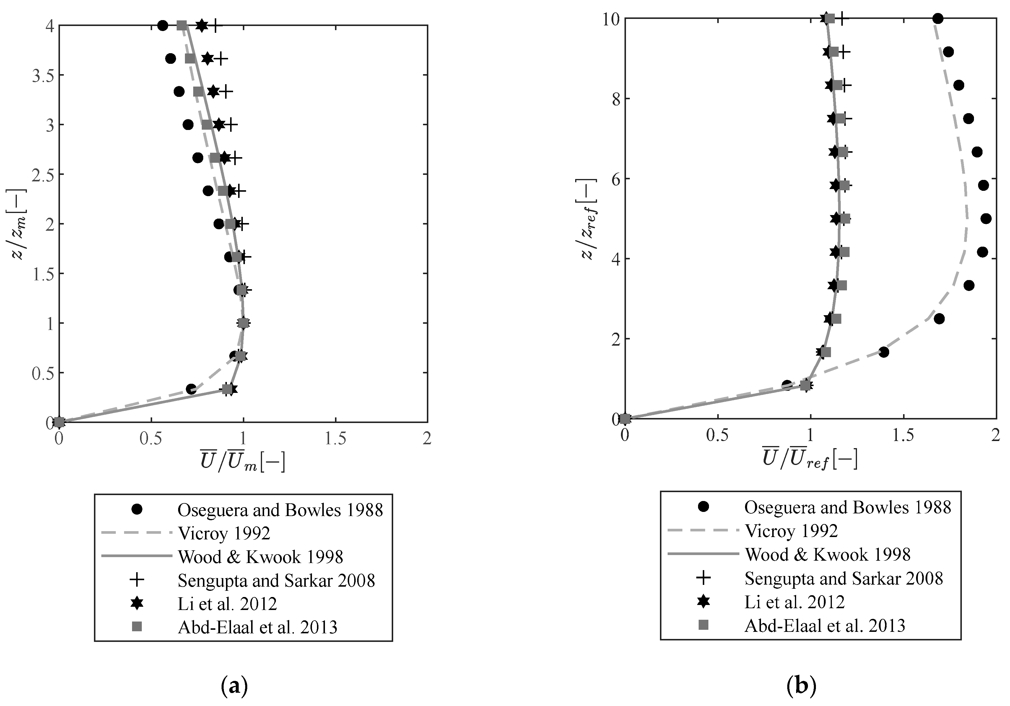
2.2. Mean Wind Velocity

Thunderstorm velocity can be described by the classical decomposition rule as the sum of a slowly varying mean wind velocity and rapidly varying turbulent fluctuation [28,29,30]. In general, the slowly varying mean wind velocity radial component U ¯ r z , r , t , is a function of the height ( z ), radial distance from the center of the downdraft ( r ) and time ( t ) [31,32,33]. The variation with the height of downburst outflow is characterized by a maximum value in the interval of 50–120 m above the ground level, showing a particular nose-like shape [2,5]. In the following paragraphs, some of the models proposed in the literature are reviewed, reporting the expressions of the vertical profile at time and radial distance ( r = r m ), where the maximum velocity appears over the whole field.
Oseguera and Bowles [34] developed an analytical model for the velocity field induced by thunderstorms based on the large-scale numerical weather model TASS. Focusing on the time and radial distance where the maximum velocity appears, the vertical profile is expressed as follows:
U ¯ z = 1.35   ·   U ¯ m e z / z * e z / ε
where, U ¯ m is the maximum mean wind speed, z * is the height at which U ¯ z * = 0.5   ·   U ¯ m , and ε is a characteristic height in the boundary layer. The authors established the relationships z m = 0.22   ·   z * , z * = 12.5   ·   ε , with z m  being the height at which the maximum wind speed U ¯ m occurs.
Vicroy [35] modified the previous empirical model through the definition of a new radial dependency, since large discrepancies with full-scale measurements were noted. He proposed the following expression:
U ¯ z = 1 , 22   ·   U ¯ m e c 1 z z m e c 2 z z m
where c 1 = 0.15  and c 2 = 3.2175 [35].
Wood and Kwok [36] proposed an empirical expression to predict the downburst wind velocity vertical profile, calibrated on laboratory tests and Computational Fluid Dynamics (CFD) simulations. After some experiments varying the distance from the impinging jet, experimental data were fitted through the following expression:
U ¯ z = A z z * B 1 erf C   ·   z z *   ·   U ¯ m
where A = 1.55 , B = 1 / 6 , C = 0.7 , erf is the error function, z * 5.5 z m ; this relationship is obtained by fixing U ¯ z * = 0.5   ·   U ¯ m in Equation (3).
Sengupta and Sarkar [37] performed impinging jet tests and measured the profiles using hotwire anemometers, pressure rakes and particle image velocimetry techniques, finding the best fit of the data for the Wood and Kwok expression, Equation (3), to be A = 1.52 , B = 1 / 6.5 , and C = 0.68 , which lead to z * 7.7 z m . In addition, good agreement was found between the empirical formulation and the full-scale measurements from the NIMROD Project and CFD numerical simulations carried out in the same work.
Li et al. [38] proposed an empirical model to obtain the vertical profile that was fitted and verified by a 3D CFD simulation. The model considers the effects of nonlinear growth of boundary layer thickness by incorporating varying characteristic length scales z m and r m as functions of the independent variables r and z , respectively. According to their model, the vertical profile of the maximum radial velocity is given by:
U ¯ z = U ¯ m z z m γ e γ 1 z z m
where γ = 0.159 and z m = 0.0393 D , D being the downburst diameter.
Abd-Elaal et al. [39] developed an empirical model based on the collection of numerical and experimental simulation results and recorded field data. The effects of nonlinear growth of boundary layer thickness were also considered by the authors. They proposed the following expression:
U ¯ z = 1.17   ·   U ¯ m z z m b 2 1 e b 1 z z m b 2  
where z m = 0.025 D , b 1 = 0.16 and b 2 = 1 1 + c 1 = 1.19 .
Figure 1 shows a comparison of the mean wind speed profiles U ¯  obtained by the analytical models presented, normalized with respect to U ¯ m (Figure 1a) and U ¯ r e f (Figure 1b), which represents the velocity at a reference height z r e f = 10   m , as functions of the height normalized with respect to z m and z r e f , respectively.
Abd-Elaal et al. [39] observed that the vertical profile from the Vicroy model shows a remarkable difference with radar observations by Hjelmfelt [5], and with the experimental and numerical simulation results for downburst wind by Wood et al. [6], Kim and Hangan [40], Sengupta and Sarkar [37]. The agreement between Wood and Kwok model and the available full-scale data is overall significantly better than that of the Vicroy model. Le and Caracoglia [31] suggested the use of Vicroy model when the maximum radial velocity is located near the ground, and of Wood and Kwok model for maximum velocity at higher elevations.

2.3. Turbulence Properties

Regarding the turbulent fluctuation, little information is available. Most scientific articles are related to the intensity of the longitudinal turbulence component, while, for the lateral and vertical components, fewer data are provided. More recent studies [2,28] have employed a directional decomposition to separate the longitudinal turbulence from the lateral one, and it has been shown that the longitudinal turbulence component derived from the classical and directional decompositions are similar.
Full-scale measurements of thunderstorms have shown that the intensity of the longitudinal turbulence component varies with time and height with a trend opposite to the mean wind speed profile [2,41]. Solari et al. [42] examined the anemometric data recorded in the ports of the Northern Tyrrhenian Sea and provided mean values for each anemometer in the ports, which range from 7% to 17% with a mean value of 12% for all of them. These low values may be related to the proximity of the wind monitoring network to the sea. However, higher values of turbulence intensity during thunderstorms were provided by Choi [43] at 10 and 20 m height in Singapore. The values at 10 m (40–65%) tend to be higher than the ones at 20 m (35–60%) for most of the directions. Canepa et al. [2] analyzed multi-point LiDAR data measured in the Livorno and Genova ports and studied the time-dependent variation along the height of the longitudinal and lateral turbulence intensity. For most thunderstorms, it was observed that, for both turbulence components, the maximum mean value of the intensity appears below the nose, and then it decreases above following different trends. However, in most cases, turbulence intensity increases again above 180 m. For each analyzed event, the mean values of the intensity of the two turbulence components were in the range of 5–12%. Romanic [44] analyzed the data measured at four heights on a tall tower and observed values around 23% near to the ground during the peak velocity, while maximum values of turbulence intensity around 30% were found to appear before the peak velocity.
Most of the full-scale measurements available correspond to anemometric records and are characterized by the uncertainty of the downdraft position with respect to the anemometer location. Turbulence intensity values at different locations with respect to the downdraft position have been provided based on experimental tests in 3D wind simulators. Zhang et al. [8] presented the variation of the longitudinal turbulence intensity along the height at different radial distances for a microburst reproduced by an impinging-jet-based microburst simulator located at Iowa State University, showing a sudden increase above 60 m in full-scale, reaching maximum values of 37% at 120 m approximately, at the radial distance r m where U ¯ m appears. However, the highest values of longitudinal turbulence intensity were observed beyond the center, ranging from 14 to 38%. Elawady et al. [45] generated a downburst wind field in the WindEEE Dome Laboratory and analyzed the vertical profile of the longitudinal turbulence intensity and its variation with the radial distance from the center of the downdraft. Values in the range of 11–14% were observed close to the location of the peak radial velocity. Canepa et al. [10] reported mean values of turbulence intensity at r m in the ranges of 8–12% during isolated downbursts reconstructed at WindEEE, while, in accordance with Zhang et al. [8], the highest values were found farther from the center (13–20%).
Since a consolidated model of the turbulence intensity profile has not been developed, it is common to consider time-averaged values of turbulence intensities as reference values. Concerning turbulence harmonic content, the residual turbulent fluctuations of thunderstorm downbursts are a non-stationary and non-Gaussian process and are commonly expressed as the product of the slowly varying standard deviation with the reduced turbulent fluctuation, e.g., [42]. Roncallo and Solari [46] showed that the reduced turbulent fluctuation can be modelled as a zero-mean stationary Gaussian random process, with a harmonic content similar to the one characterizing synoptic events. Statistical analysis of the multi-point turbulence field during thunderstorms have not been carried out in the literature, so a suitable model of the turbulence coherence function is not currently available.

3. Experimental Setup

The tests were carried out at the Giovanni Solari Wind Tunnel (WT) facility at the University of Genoa, which is a closed-circuit traditional atmospheric boundary layer WT (Figure 2). Its cross-section is rectangular, 1.70 m (width) × 1.35 m (height), and the working section is 8.80 m long. The controllable wind speed range is 0.2–32 m/s.
Atmospheric turbulent boundary layers are generally set up using an arrangement of roughness elements, distributed over the floor of the wind tunnel, and two-dimensional elements (spires and a fence) located at the inlet of the test section (Figure 3a). In order to reproduce the nose-shaped profile of a thunderstorm, a partial grid (TS grid) has been specifically designed based on practical experience, using preliminary work [47] as a foundation for the design process. The basic idea is to lower the flow velocity at the upper part of the test chamber, aiming to replicate the characteristic nose-shaped mean wind profile. To achieve this, modules with variable opening sizes were designed, allowing for variations in the shape of the profile, the height of the nose and the level of turbulence intensity. The TS grid is composed by different rectangular modules spanning the full width of the wind tunnel and including square openings of different dimensions. Currently, the laboratory is equipped with six modules, two by two, with small, intermediate and large openings, corresponding to porosities of about 40%, 45% and 50%, respectively. The partial grid is installed 4 m downstream of the WT inlet section and covers approximately two thirds of the height of the WT test section, as shown in Figure 3b.
A geometrical scale of 1:400 was considered, based on the idea of using this setup for testing a tall building in future works. During the experiments, a dynamic multi-hole pressure probe (i.e., TFI Cobra probe) was used for measuring the flow three-component velocity fluctuations with a sampling frequency of 2 kHz. The accuracy of measurements was generally within ±0.5 m/s and ±1° pitch and yaw angle, up to about 30% turbulence intensity. The Cobra probe range of measurement was from 2 to 100 m/s within a ±45° cone of its x-axis. The three components of the wind speed time histories were acquired approximately 3 m downstream from the TS grid’s position for a number of key locations along the height of the wind tunnel. From the measured time histories, mean wind speed and longitudinal turbulence intensity profiles were derived.
The experimental tests aimed to simulate the nose-like feature of the mean velocity vertical profile at the radial location where the maximum wind speed occurs, neglecting the unsteady characteristics of thunderstorm-downbursts. The measured mean wind speed profiles were compared with the analytical model developed by Wood and Kwok, Equation (3), for different heights of the nose. Two configurations of the roughness elements were considered, while several arrangements of the TS grid modules were tested in order to evaluate their influence on the shape of the mean wind speed profiles.

4. Results and Discussion

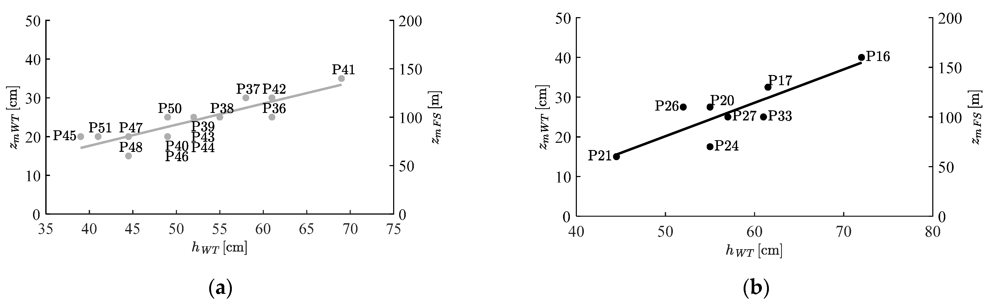
4.1. Mean Wind Velocity Profile

The distance h between the floor of the wind tunnel and the bottom of the TS grid module was varied and different arrangements of the TS grid modules were tested. Figure 4 shows the height of the nose z m obtained as a function of h . The left-hand side of the y-axis shows the values of z m in the wind tunnel ( z m W T ) , while the right-hand side shows the corresponding full-scale values ( z m F S ) . P## in Figure 4 indicates the Profile no. ##, corresponding to the different arrangements tested during the current WT test campaign. The two different setups correspond to different extensions of the roughness elements on the floor and different heights of the fence (Roughness 1, Figure 4a, Roughness 2, Figure 4b). Measurements are made at the center of the turntable in the environmental test section of the Giovanni Solari Wind Tunnel.
For both roughness configurations, it can be observed that, by increasing the separation distance h of the modules from the WT floor, the height of the nose z m increases, achieving a large range of possible values for this parameter. The same value of z m can be obtained also for different values of h, depending on the porosity of the TS grid modules closer to the floor. It should be noted that the full-scale height of the tip of the nose, as depicted on the right-hand side of the y-axis in Figure 4, is evaluated based on the target geometrical scale of 1:400. For larger scales, the adopted setups would correspond to lower heights of the nose tip in full scale. However, the obtained results have shown that the height of the nose is nearly proportional to the distance h between the wind tunnel floor and the bottom of the lowest grid. Consequently, to achieve heights of the nose tip typical of thunderstorm downbursts for larger geometrical scales, the distance between the wind tunnel floor and the bottom of the lowest grid should be appropriately increased.
Figure 5 shows the measured profiles that best match the Wood and Kwok target profile for three heights of the nose, i.e., z m = 60 , 80 and 100 m in full-scale; 10% confidence lines with respect to the target profile are also plotted.
The graphs show a good agreement between the target and measured profiles within the confidence lines; however, it can be seen that, for heights above 150 m, the measured profiles start to differ from the target, providing lower velocities.

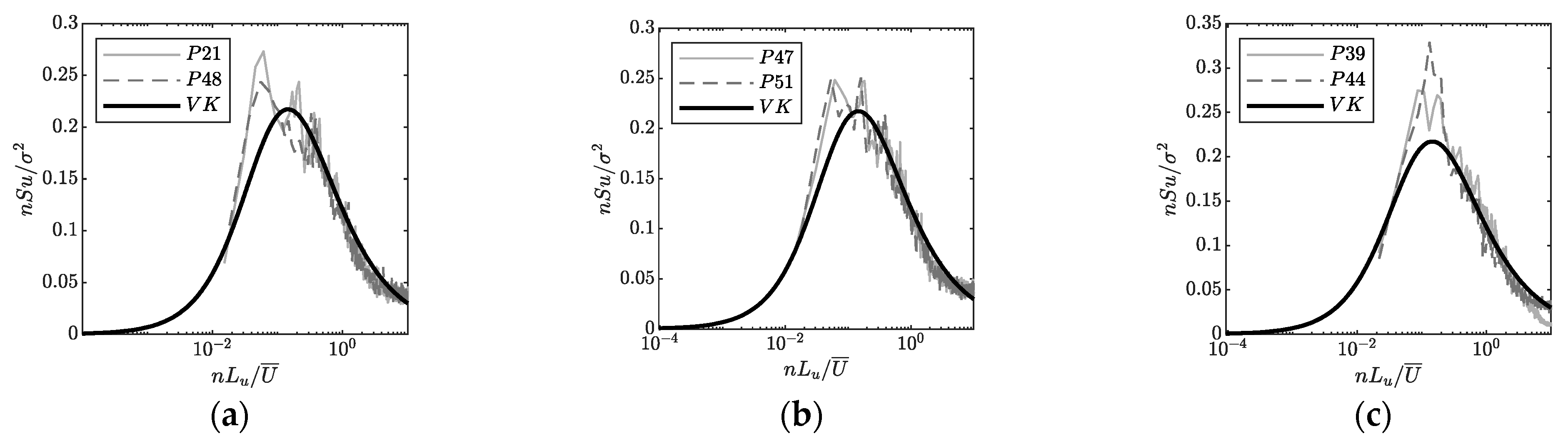
4.2. Turbulence Intensity Properties

Due to the lack of a defined target profile for the longitudinal turbulence intensity, only realistic variation with height was checked, opposite to the trend of the mean wind speed profile, as pointed out in Section 2.3. Figure 6 shows the longitudinal turbulence intensity profiles for the measured mean wind speed profiles reported in Section 4.1.
The trend of turbulence intensity with the height is in accordance with full-scale [2] and scaled [8,10] measurements. In addition, it can be noticed that different levels of turbulence intensity can be achieved by modifying the roughness elements and the arrangement of the TS grid modules. Figure 7 shows the setups corresponding to the profiles plot in Figure 5 and Figure 6. Lower turbulence intensities were obtained for the configurations corresponding to the profiles P21, P47 and P39, varying in a range between 8% and 12%, while for the other configurations, higher values were obtained, mainly for P44. In the cases of the profiles with z m = 60 m (Figure 6a), the differences between the two configurations are the roughness elements and the addition in the inlet section, for P48, of a classic wooden grid to generate turbulence, which covers the entire area of the WT section (Figure 7a bottom). Figure 6b shows greater differences between turbulence intensities for heights above 60 m, and this may be related to the fact that the TS module closest to the WT roof was removed for P51, leaving it as an empty space (Figure 7b bottom). In Figure 6c, the increase in turbulence intensity can be detected for all heights: in P44, the two TS modules closest to the WT roof were removed with respect to P39 (Figure 7c). Overall, the tests have shown that is possible to obtain a mean wind speed profile in agreement with the Wood and Kwok model and to achieve different ranges of turbulence intensities.
Considering that the used passive device can not reproduce the non-stationary characteristics of thunderstorms, stationary turbulence characteristics are obtained, corresponding to the reduced turbulence fluctuation. The literature is consistent in affirming that the PSD of the reduced turbulent fluctuation of thunderstorms has similar properties to the classical PSD of synoptic events (e.g., [3,42]). Figure 8 shows the PSD of the longitudinal turbulence component at the height of the nose for the configurations analyzed in this Section, compared with the Von Karman model (VK).
A good agreement between the PSD of the recorded turbulence and the Von Karman model was verified, confirming that also the harmonic content of the simulated turbulence is in line with literature models.
As a final point, it should be noted that the TS grids are installed relatively close to the WT test section where measurements on models would be performed. This proximity could potentially make the profile unstable or, in other words, vary within the turntable, leading to potentially inaccurate measurements. Therefore, additional measurements of wind profiles were conducted in order to verify the uniformity and symmetry of the flow within the turntable. Time histories of wind velocity were measured at four locations over the turntable, as shown in Figure 9a. As a test case, Figure 9b shows the comparison between the measured profiles (P21) for different positions of the probe.
A very good agreement between the measured profiles for the different locations can be observed in Figure 9b, confirming the stability of the mean wind speed and turbulence intensity profiles over the turntable. Uniformity of the profile was also checked and verified for the configurations corresponding to all the profiles analyzed in this Section.

5. Conclusions

This paper provides a description and analysis of a series of experiments performed in the Giovanni Solari Wind Tunnel at the University of Genoa in order to reproduce thunderstorm mean wind velocity and turbulence intensity profiles. In addition to standard devices, a specific grid-like device was designed in order to reproduce the nose-shape of the mean wind speed profile. The resulting measurements in terms of mean wind speed were found to fit well the target profile (i.e., the Wood and Kwok empirical model). It was found that different configurations of the modules provided a large range of variation for the height of the nose that could be significant for different types of structures, especially for tall buildings. In terms of turbulence intensity, despite the lack of an analytical model, the profiles obtained were considered to be acceptable based on existing experimental and full-scale measurements. The solution also appears very satisfactory in terms of flow uniformity. These results demonstrate that the nose shape of the mean wind velocity profile can be effectively generated in a traditional wind tunnel using a passive modular grid, which is a relatively simple and cost-effective way to simulate wind characteristics for WT testing on scaled structures. In conclusion, the proposed device offers a practical solution for the experimental simulation of nose-shaped profiles in order to evaluate thunderstorm-induced wind loads on structures using common geometric scales for building tests (e.g., 1:400). By employing various configurations of the grid modules, the device can be adapted to facilitate testing at smaller geometric scales, broadening its range of applicability. Moreover, it provides a more affordable approach for technical projects with respect to sophisticated solutions due to its simplicity and low cost. It is evident that the adopted setup lacks the ability to reproduce the non-stationarity features of thunderstorms, which may be crucial when conducting a detailed assessment of the thunderstorm loading on a structure. A comparison with experimental tests carried out with active grids, able to reproduce the main non-stationary features of thunderstorms, would enable an evaluation of their effective influence on the assessment of thunderstorm-induced loading on structures.

Author Contributions

Conceptualization: C.A.S. and F.T.; Methodology: A.B., C.A.S., F.T. and G.P.; Software: C.A.S.; Validation: A.B. and F.T.; Formal Analysis: C.A.S.; Investigation: C.A.S. and F.T.; Resources: A.B. and G.P.; Data Curation, C.A.S. and F.T.; Writing—Original Draft Preparation: C.A.S.; Writing—Review and Editing: A.B., F.T. and G.P.; Visualization: A.B. and C.A.S.; Supervision: A.B., F.T. and G.P. All authors have read and agreed to the published version of the manuscript.

Funding

This study was carried out within the RETURN Extended Partnership and received funding from the European Union Next-Generation EU (National Recovery and Resilience Plan—NRRP, Mission 4, Component 2, Investment 1.3—D.D. 1243 2/8/2022, PE0000005). The first author has a PhD scholarship financed by PON Project: “Programma Operativo Nazionale Ricerca e Innovazione 2014–2020 (CCI 2014IT16M2OP005)”, risorse FSE REACT-EU, Azione IV.4 “Dottorati e contratti di ricerca su tematiche dell’innovazione” e Azione IV.5 “Dottorati su tematiche Green”.

Institutional Review Board Statement

Not applicable.

Informed Consent Statement

Not applicable.

Data Availability Statement

Data sharing not applicable (all relevant data is presented and included within the paper).

Acknowledgments

The authors gratefully acknowledge Stefano Torre and Edoardo Ruffini for the technical support during the wind tunnel experiments.

Conflicts of Interest

The authors declare no conflict of interest.

References

  1. Fujita, T. The Downburst: Microburst and Microburst; University of Chicago: Chicago, IL, USA, 1985. [Google Scholar]
  2. Canepa, F.; Burlando, M.; Solari, G. Vertical profile characteristics of thunderstorm outflows. J. Wind Eng. Ind. Aerodyn. 2020, 206, 104332. [Google Scholar] [CrossRef]
  3. Solari, G.; Burlando, M.; Repetto, M.P. Detection, simulation, modelling and loading of thunderstorm outflows to design wind-safer and cost-efficient structures. J. Wind Eng. Ind. Aerodyn. 2020, 200, 104142. [Google Scholar] [CrossRef]
  4. Solari, G. Thunderstorm Downbursts and Wind Loading of Structures: Progress and Prospect. Front. Built Environ. 2020, 6, 63. [Google Scholar] [CrossRef]
  5. Hjelmfelt, M.R. Structure and Life Cycle of Microburst Outflows Observed in Colorado. J. Appl. Meteorol. 1988, 27, 900–927. [Google Scholar] [CrossRef]
  6. Wood, G.S.; Kwok, K.C.; Motteram, N.A.; Fletcher, D.F. Physical and numerical modelling of thunderstorm downbursts. J. Wind Eng. Ind. Aerodyn. 2001, 89, 535–552. [Google Scholar] [CrossRef]
  7. Romanic, D.; Parvu, D.; Hangan, H. Downburst reconstruction using physical simulation and analytical model with application to urban environments. In Proceedings of the International Conference on Urban Physics, Quito-Gálapagos, Ecuador, 26–30 September 2016. [Google Scholar] [CrossRef]
  8. Zhang, Y.; Sarkar, P.; Hu, H. An experimental study on wind loads acting on a high-rise building model induced by microburst-like winds. J. Fluids Struct. 2014, 50, 547–564. [Google Scholar] [CrossRef]
  9. Irwin, P.A. Wind engineering challenges of the new generation of super-tall buildings. J. Wind Eng. Ind. Aerodyn. 2009, 97, 328–334. [Google Scholar] [CrossRef]
  10. Canepa, F.; Burlando, M.; Romanic, D.; Solari, G.; Hangan, H. Experimental investigation of the near-surface flow dynamics in downburst-like impinging jets. Environ. Fluid Mech. 2022, 22, 921–954. [Google Scholar] [CrossRef]
  11. Aboutabikh, M.; Ghazal, T.; Chen, J.; Elgamal, S.; Aboshosha, H. Designing a blade-system to generate downburst outflows at boundary layer wind tunnel. J. Wind Eng. Ind. Aerodyn. 2019, 186, 169–191. [Google Scholar] [CrossRef]
  12. Le, V.; Caracoglia, L. Generation and characterization of a non-stationary flow field in a small-scale wind tunnel using a multi-blade flow device. J. Wind Eng. Ind. Aerodyn. 2019, 186, 1–16. [Google Scholar] [CrossRef]
  13. Butler, K.; Cao, S.; Kareem, A.; Tamura, Y.; Ozono, S. Surface pressure and wind load characteristics on prisms immersed in a simulated transient gust front flow field. J. Wind Eng. Ind. Aerodyn. 2010, 98, 299–316. [Google Scholar] [CrossRef]
  14. Mason, M.S.; Lo, Y. Wind loading of the CAARC building during velocity profile transitions, Part 1: Transient pressure coefficient distributions. In Proceedings of the 15th International Conference on Wind Engineering, Beijing, China, 16 September 2019; pp. 829–830. [Google Scholar]
  15. Burlando, M.; Romanic, D. Groundbreaking contributions to downburst monitoring, modeling, and detection. In The Oxford Handbook of Non-Synoptic Wind Storms; Hangan, H., Kareem, A., Eds.; Oxford University Press: New York, NY, USA, 2020. [Google Scholar] [CrossRef]
  16. Jubayer, C.; Elatar, A.; Hangan, H. Pressure distributions on a low-rise building in a laboratory simulated downburst. In Proceedings of the 8th International Colloquium on Bluff Body Aerodynamics and Applications Northeastern University, Boston, MA, USA, 7–11 June 2016. [Google Scholar]
  17. Letchford, C.; Chay, M. Pressure distributions on a cube in a simulated thunderstorm downburst. Part B: Moving downburst observations. J. Wind Eng. Ind. Aerodyn. 2002, 90, 733–753. [Google Scholar] [CrossRef]
  18. Asano, K.; Iida, Y.; Uematsu, Y. Laboratory study of wind loads on a low-rise building in a downburst using a moving pulsed jet simulator and their comparison with other types of simulators. J. Wind Eng. Ind. Aerodyn. 2019, 184, 313–320. [Google Scholar] [CrossRef]
  19. Canepa, F.; Burlando, M.; Hangan, H.; Romanic, D. Experimental Investigation of the Near-Surface Flow Dynamics in Downburst-like Impinging Jets Immersed in ABL-like Winds. Atmosphere 2022, 13, 621. [Google Scholar] [CrossRef]
  20. Romanic, D.; Ballestracci, A.; Canepa, F.; Solari, G.; Hangan, H. Aerodynamic coefficients and pressure distribution on two circular cylinders with free end immersed in experimentally produced downburst-like outflows. Adv. Struct. Eng. 2020, 24, 522–538. [Google Scholar] [CrossRef]
  21. Butler, K.; Kareem, A. Physical and numerical modeling of downburst generated gust fronts. In Proceedings of the 12th International Conference on Wind Engineering, Cairns, Australia, 2–6 July 2007. [Google Scholar]
  22. Mejia, A.; Vutukuru, K.; Elawady, A.; Chowdhury, A.; Irwin, P. Downburst simulations at The NHERI Wall of Wind experimental facility. In Proceedings of the 15th International Conference on Wind Engineering, Bejing, China, 1–6 September 2019. [Google Scholar]
  23. Levieux, G.; Elawady, A.; Chowdhury, A.; Aloui, F. 2D Numerical simulation of downburst simulator in the Wall of Wind. In Energy and Exergy for Sustainable and Clean Environment; Geo, V.E., Aloui, F., Eds.; Springer Nature Singapore: Singapore, 2023; Volume 2. [Google Scholar]
  24. Alawode, K.; Elawady, A.; Shafieezadeh, A.; Chowdhury, A.; Azzi, Z. Aerolastic testing to examine the dynamic behavior of a single self-supported electrical transmission tower subjected to downburst wind loads. In Proceedings of the 14th Americas Conference on Wind Engineering, Lubbock, TX, USA, 17–19 May 2022. [Google Scholar]
  25. Zhao, Y.; Cao, S.; Tamura, Y.; Duan, Z.; Ozono, S. Simulation of downburst in a multiple fan wind tunnel and research on its load on high-rise structure by wind tunnel experiment. In Proceedings of the International Conference on Mechatronics and Automaion, Changchun, China, 9–12 August 2009. [Google Scholar]
  26. Ma, R.; Zhou, Q.; Wang, P.; Yang, Y.; Li, M.; Cao, S. Effects of sinusoidal streamwise gust on the vortex-induced force on an oscillating 5:1 rectangular cylinder. J. Wind Eng. Ind. Aerodyn. 2021, 213, 104642. [Google Scholar] [CrossRef]
  27. Li, S.; Snaiki, R.; Wu, T. Active Simulation of Transient Wind Field in a Multiple-Fan Wind Tunnel via Deep Reinforcement Learning. J. Eng. Mech. 2021, 147, 04021056. [Google Scholar] [CrossRef]
  28. Zhang, S.; Solari, G.; Burlando, M.; Yang, Q. Directional decomposition and properties of thunderstorm outflows. J. Wind Eng. Ind. Aerodyn. 2019, 189, 71–90. [Google Scholar] [CrossRef]
  29. Tubino, F.; Solari, G. Time varying mean extraction for stationary and nonstationary winds. J. Wind Eng. Ind. Aerodyn. 2020, 203, 104187. [Google Scholar] [CrossRef]
  30. Brusco, S.; Buresti, G.; Piccardo, G. Thunderstorm-induced mean wind velocities and accelerations through the continuous wavelet transform. J. Wind Eng. Ind. Aerodyn. 2022, 221, 104886. [Google Scholar] [CrossRef]
  31. Le, T.-H.; Caracoglia, L. Computer-based model for the transient dynamics of a tall building during digitally simulated Andrews AFB thunderstorm. Comput. Struct. 2017, 193, 44–72. [Google Scholar] [CrossRef]
  32. Chay, M.; Albermani, F.; Wilson, R. Numerical and analytical simulation of downburst wind loads. Eng. Struct. 2006, 28, 240–254. [Google Scholar] [CrossRef] [Green Version]
  33. Xhelaj, A.; Burlando, M.; Solari, G. A general-purpose analytical model for reconstructing the thunderstorm outflows of travelling downbursts immersed in ABL flows. J. Wind Eng. Ind. Aerodyn. 2020, 207, 104373. [Google Scholar] [CrossRef]
  34. Oseguera, R.M.; Bowles, R.L. A Simple, Analytic 3-Dimensional Downburst Model Based on Boundary Layer Stagnation Flow; NASA Technical Memorandum 100632; NASA: Hampton, VA, USA, 1988. [Google Scholar]
  35. Vicroy, D.D. Assessment of microburst models for downdraft estimation. J. Aircr. 1992, 29, 1043–1048. [Google Scholar] [CrossRef]
  36. Wood, S.; Kwok, K. An empirically derived estimate for the mean velocity profile of a thunderstorm downburst. In Proceedings of the 7th Australian Wind Engineering Society Workshop, Auckland, New Zealand, 28–29 September 1998. [Google Scholar]
  37. Sengupta, A.; Sarkar, P.P. Experimental measurement and numerical simulation of an impinging jet with application to thunderstorm microburst winds. J. Wind Eng. Ind. Aerodyn. 2008, 96, 345–365. [Google Scholar] [CrossRef]
  38. Li, C.; Li, Q.; Xiao, Y.; Ou, J. A revised empirical model and CFD simulations for 3D axisymmetric steady-state flows of downbursts and impinging jets. J. Wind Eng. Ind. Aerodyn. 2012, 102, 48–60. [Google Scholar] [CrossRef]
  39. Abd-Elaal, E.-S.; Mills, J.E.; Ma, X. An analytical model for simulating steady state flows of downburst. J. Wind Eng. Ind. Aerodyn. 2013, 115, 53–64. [Google Scholar] [CrossRef]
  40. Kim, J.; Hangan, H. Numerical simulations of impinging jets with application to downbursts. J. Wind Eng. Ind. Aerodyn. 2007, 95, 279–298. [Google Scholar] [CrossRef]
  41. Durañona, V.; Sterling, M.; Baker, C. An analysis of extreme non-synoptic winds. J. Wind Eng. Ind. Aerodyn. 2007, 95, 1007–1027. [Google Scholar] [CrossRef]
  42. Solari, G.; Burlando, M.; De Gaetano, P.; Repetto, M.P. Characteristics of thunderstorms relevant to the wind loading of structures. Wind Struct. 2015, 20, 763–791. [Google Scholar] [CrossRef]
  43. Choi, E.C. Wind characteristics of tropical thunderstorms. J. Wind Eng. Ind. Aerodyn. 2000, 84, 215–226. [Google Scholar] [CrossRef]
  44. Romanic, D. Mean flow and turbulence characteristics of a nocturnal downburst recorded on a 213 m tall meteorological tower. J. Atmos. Sci. 2021, 78, 3629–3650. [Google Scholar] [CrossRef]
  45. Elawady, A.; Aboshosha, H.; El Damatty, A.; Bitsuamlak, G.; Hangan, H.; Elatar, A. Aero-elastic testing of multi-spanned transmission line subjected to downbursts. J. Wind Eng. Ind. Aerodyn. 2017, 169, 194–216. [Google Scholar] [CrossRef]
  46. Roncallo, L.; Solari, G. An evolutionary power spectral density model of thunderstorm outflows consistent with real-scale time-history records. J. Wind Eng. Ind. Aerodyn. 2020, 203, 104204. [Google Scholar] [CrossRef]
  47. Aurelius, L.; Buttgereit, V.; Cammelli, S.; Zanina, M. The impact of Shamal winds on tall building design in the Gulf Region. In Proceedings of the International Conference on Tall Buildings: Architectural and Structural Advances, ACI, Abu Dhabi, United Arab Emirates, 6 February–5 April 2008. [Google Scholar]
Figure 1. Comparison of the normalized mean wind speed profile [34,35,36,37,38,39]: (a) U ¯ / U ¯ m ; (b) U ¯ / U ¯ r e f .
Applsci 13 08064 g001
Figure 2. The Giovanni Solari Wind Tunnel at the University of Genoa.
Applsci 13 08064 g002
Figure 3. Devices used to reproduce a thunderstorm’s vertical profile: (a) Traditional devices; (b) New passive device to reproduce the nose-shaped mean wind speed profile of a downburst.
Applsci 13 08064 g003
Figure 4. Variation of z m with h : (a) Roughness 1; (b) Roughness 2. Legend: P## (P: profile, ##: test number).
Applsci 13 08064 g004
Figure 5. Measured wind speed profiles vs. target profile: (a) z m = 60   m ; (b) z m = 80   m ; (c) z m = 100   m .
Applsci 13 08064 g005
Figure 6. Measured longitudinal turbulence intensity profiles: (a) z m = 60   m ; (b) z m = 80   m ; (c) z m = 100   m .
Applsci 13 08064 g006
Figure 7. Setups corresponding to the profiles (a) P21 (top) and P48 (bottom); (b) P47 (top) and P51 (bottom); (c) P39 (top) and P44 (bottom).
Applsci 13 08064 g007
Figure 8. PSD of the measured reduced fluctuations and Von Karman model: (a) z m = 60   m ; (b) z m = 80   m ; (c) z m = 100   m .
Applsci 13 08064 g008
Figure 9. (a) Cobra probe coordinates over the turntable; (b) Comparison between the measured profiles for the configuration P21 (x = 0 y = 0 corresponds to the turntable center).
Applsci 13 08064 g009
Disclaimer/Publisher’s Note: The statements, opinions and data contained in all publications are solely those of the individual author(s) and contributor(s) and not of MDPI and/or the editor(s). MDPI and/or the editor(s) disclaim responsibility for any injury to people or property resulting from any ideas, methods, instructions or products referred to in the content.

