
Low-Light Image Enhancement Method for Electric Power Operation Sites Considering Strong Light Suppression
School of Computer Science, Northeast Electric Power University, Jilin 132012, China
*
Author to whom correspondence should be addressed.
Appl. Sci. 2023, 13(17), 9645; https://0-doi-org.brum.beds.ac.uk/10.3390/app13179645
Submission received: 25 July 2023
/
Revised: 18 August 2023
/
Accepted: 24 August 2023
/
Published: 25 August 2023
(This article belongs to the Special Issue Image Enhancement and Restoration Based on Deep Learning Technology)
Abstract
:Insufficient light, uneven light, backlighting, and other problems lead to poor visibility of the image of an electric power operation site. Most of the current methods directly enhance the low-light image while ignoring local strong light that may appear in the electric power operation site, resulting in overexposure and a poor enhancement effect. Aiming at the above problems, we propose a low-light image enhancement method for electric power operation sites by considering strong light suppression. Firstly, a sliding-window-based strong light judgment method was designed, which used a sliding window to segment the image, and a brightness judgment was performed based on the average value of the deviation and the average deviation of the subimages of the grayscale image from the strong light threshold. Then, a light effect decomposition method based on a layer decomposition network was used to decompose the light effect of RGB images with the presence of strong light and eliminate the light effect layer. Finally, a Zero-DCE (Zero-Reference Deep Curve Estimation) low-light enhancement network based on a kernel selection module was constructed to enhance the low-light images with reduced or no strong light interference. Comparison experiments using the electric power operation private dataset and the SICE (Single Image Contrast Enhancement) Part 2 public dataset showed that our proposed method outperformed the current state-of-the-art low-light enhancement methods in terms of both subjective visual effects and objective evaluation metrics, which effectively improves the image quality of electric power operation sites in low-light environments and provides excellent image bases for other computer vision tasks, such as the estimation of operators’ posture.
1. Introduction
Intelligent video surveillance systems are frequently utilized in electric power operation settings as a result of the advancement of computer vision and other artificial intelligence technologies. Affected by weather, light, and other influences, there are problems such as insufficient light, uneven light, and backlight in the electric power operation scene, which leads to poor image visibility, and the low-light image seriously affects the accuracy of target detection and operator-behavior recognition tasks in the operation scene. Figure 1 shows a comparison of low-light and normal images and their grayscale histograms at an electric power operation site. A large number of misdetections and omissions occur in low-light images (a) and (b) for the detection of skeletal keypoints of electric power operators, which seriously affects the use of skeletal keypoints in the behavioral monitoring of operators. Comparing the grayscale histograms, the grayscale histograms of the low-light images show uneven pixel distribution, with pixels of a smaller grayscale accounting for most of the pixels, while the grayscale distribution of the normal image (c) is more balanced. Therefore, studying the low-light image enhancement method for electric power operation sites is crucial for item detection and personnel behavior recognition at the operation site.
Due to the special characteristics of the electric power industry, strong light sources are often used to augment light operations at night; for example, in Figure 1 image (d), although the strong light source enhances the local brightness, it interferes with the low-light enhancement, resulting in local overexposure. So, the low-light image enhancement of the electric power operation site needs to be considered as a suppression of the strong light effect.
For electric power operation sites, we suggest a low-light image enhancement method that takes strong light suppression into account, which is different from other current low-light enhancement methods from the perspective of practical applications in electric power operation, and considers both the overall low-light image and the presence of a strong light source in low light. Our contributions are summarized as follows:
- We designed a strong light judgment method based on sliding windows, which used a sliding window to segment the image; a brightness judgment was performed based on the average value of the deviation and the average deviation of the subimages of the grayscale image from the strong light threshold in order to search for strong light.
- We used a light effect decomposition method based on a layer decomposition network to decompose the light effects of RGB images in the presence of strong light to eliminate the light effect layer and to reduce the interference of strong light effects on the enhancement of low-light images.
- We constructed a Zero-DCE low-light enhancement network based on a kernel selection module, with a significant decrease in the number of parameters (Params) and the number of floating-point operations (FLOPs) compared with the original Zero-DCE; the subjective visual quality and objective evaluation metrics of the enhanced images outperformed those of other current state-of-the-art methods.
2. Related Work
The weather, light, and other environmental factors frequently have an impact on the image quality in real settings, which causes some image information to vanish in the dark and present low light. Traditional enhancement methods and deep-learning-based enhancement methods make up the two primary categories of low-light picture improvement research.
The histogram equalization [1], gamma correction [2], and Retinex theory [3]-based conventional low-light image enhancing methods are among the more reliable ones. Among them, histogram equalization stretches the grayscale histogram of the image from a more concentrated grayscale interval to the entire grayscale range, expanding the range of grayscale values in the image and improving the image contrast and part of the detail effect, but it is prone to chromatic aberration and the grayscale merging loses the detail information. Gamma correction adjusts the parameters to change the magnitude of the enhancement of the image luminance by a non-linear function, which also loses the detail information and generates a large amount of noise. The theoretical basis of the Retinex model is the three-color theory and color constancy, which removes or reduces the influence of the incident image by the same method to preserve the image of the essential reflective properties of the object as much as possible. Retinex theory has been the subject of ongoing research, leading to the development of algorithms like SSR (single-scale Retinex) [4], MSR (multi-scale Retinex) [5], and MSRCR (multi-scale Retinex with color recovery) [6]. Traditional algorithms have the advantages of a fast processing speed and easy deployment, but they lack references to real lighting conditions and suffer from problems such as noise being retained or amplified, artifacts, and color deviations.
From both supervised and unsupervised learning viewpoints, low-light image enhancement methods based on deep learning can be distinguished. Lore et al. proposed LLNet (Low-Light Net) [7] for supervised learning. This network adopts the traditional self-encoder and decoder structures and improves image contrast and denoising by stacking sparse denoising self-encoders, but in order to easily obtain the paired dataset, artificially synthesized low light and noise images are used during the training process, which leads to poor generalization ability and enhancement effects in real scenes. RetinexNet [8], a convolutional neural network approach that Wei et al. proposed, is based on the Retinex theory. The input image is segmented into reflection and illumination maps by a Decom-Net subnetwork and the Enhance-Net subnetwork is utilized to adjust and estimate the illumination maps in order to obtain the image after boosting the contrast. Limited by the ideal state of Retinex theory, this algorithm suffers from serious color deviation problems when enhancing extremely dark light images and multi-color light night images. To correct exposure and underexposure from coarse to fine, Afifi et al. presented LMSPEC (Learning Multi-Scale Photo Exposure Correction) [9], which formulated the exposure correction problem as two subproblems—color enhancement and detail enhancement—and used a DNN (deep neural network) model, which was trained in an end-to-end manner to correct global color information first and then improve image details; however, the network design was too complex and the network was not able to constrain the color information of a region of an image when the region was completely saturated. In the field of unsupervised learning, EnlightenGAN [10] is a low-light image improvement technique proposed by Jiang et al., based on a generative adversarial network (GAN). It includes a U-Net with an attention mechanism as a generator and a pair of “global–local” discriminators [11]. So that the low-light image may be converted back into a high-contrast image, the generator is trained by evaluating the difference feedback between the discriminator and the normal light HD image. EnlightenGAN solves the problem of not having easy access to “paired datasets” in supervised learning. Considering that GAN-based algorithms are not stable during the training process, Guo et al. proposed Zero-DCE [12] from the point of view of image depth profile estimation, designing a higher-order depth curve that could automatically map a dark light image to an enhanced version, LE. By estimating the depth higher-order curve of the input image, the LE curve is used as the target to guide the network in pixel level adjustment of low-light images. The Zero-DCE network structure is designed to be simple, able to train image datasets of different scenes quickly, and has a strong generalization capability. Jin et al. [13] proposed an unsupervised method by combining layer decomposition with light effect suppression; namely, UNIE (Unsupervised Night Image Enhancement). The decomposition network learns to decompose the light effect as well as shading and reflectance layers under the guidance of an unsupervised specific prior loss. The light effect suppression network further suppresses the light effect while enhancing the illumination of dark regions; structural and high-frequency coherence losses were proposed in order to recover background details and reduce illusions and artifacts. Radulescu et al. [14] decomposed an image into representations in the frequency domain in order to refine the image rendering. Various image decomposition methods provide new ideas for the light effect decomposition of the special power operation site in this paper.
3. Methods
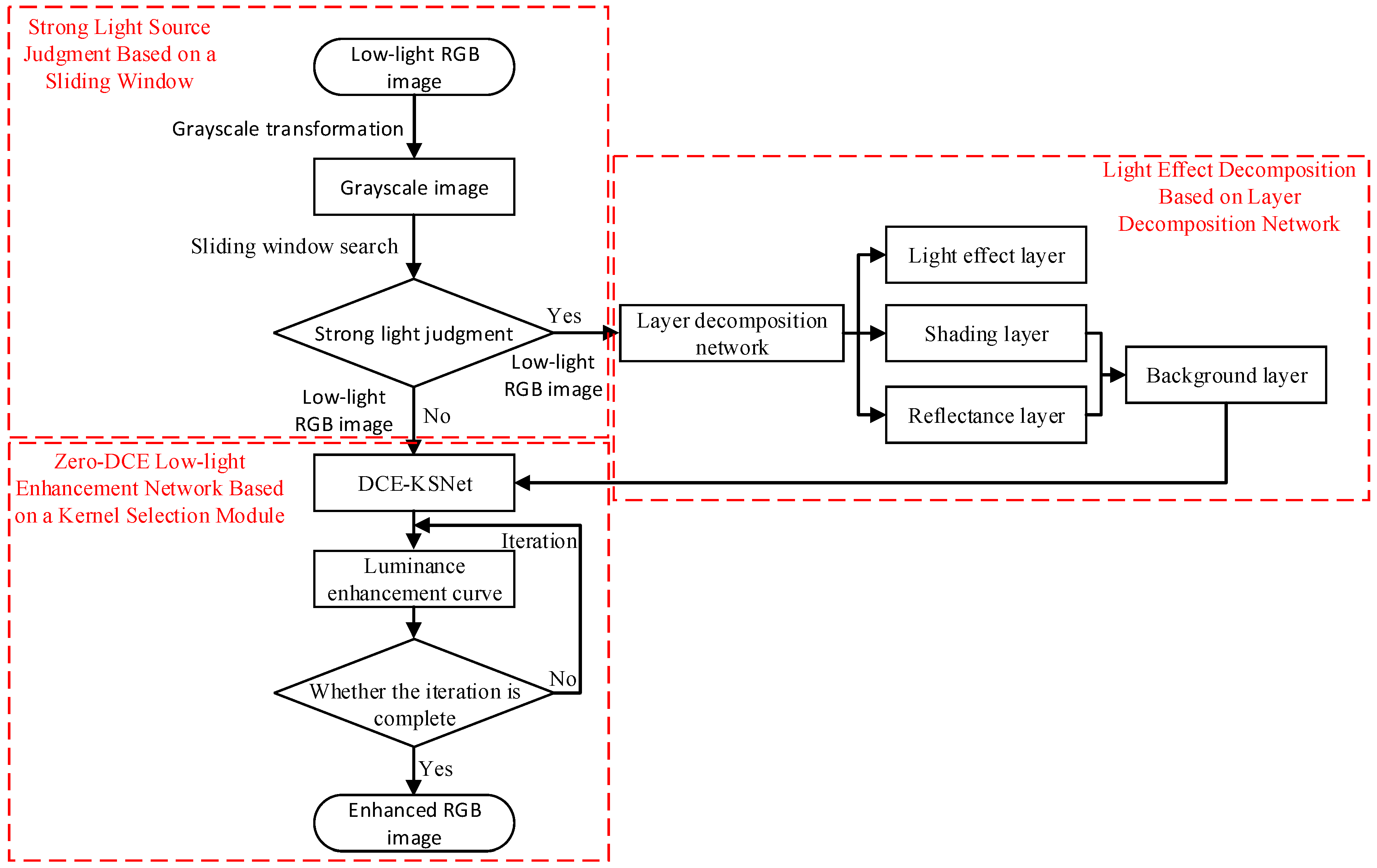
We suggest a low-light image enhancement method for electric power operation sites considering strong light suppression, which includes a strong light judgment based on a sliding window, light effect decomposition based on a layer decomposition network, and Zero-DCE low-light enhancement based on a kernel selection module. For the input low-light RGB image, a sliding window is used to search the image after grayscale transformation and judge the strong light region; the layer decomposition network is used to decompose the light effect of the strong light image and obtain the background layer after the removal of the light effect layer. The low-light enhancement of the background layer image is realized based on the Zero-DCE network of the kernel selection module. The overall flowchart of the low-light image enhancement method for electric power operation sites considering strong light suppression is shown in Figure 2.
3.1. Strong Light Source Judgment Based on a Sliding Window
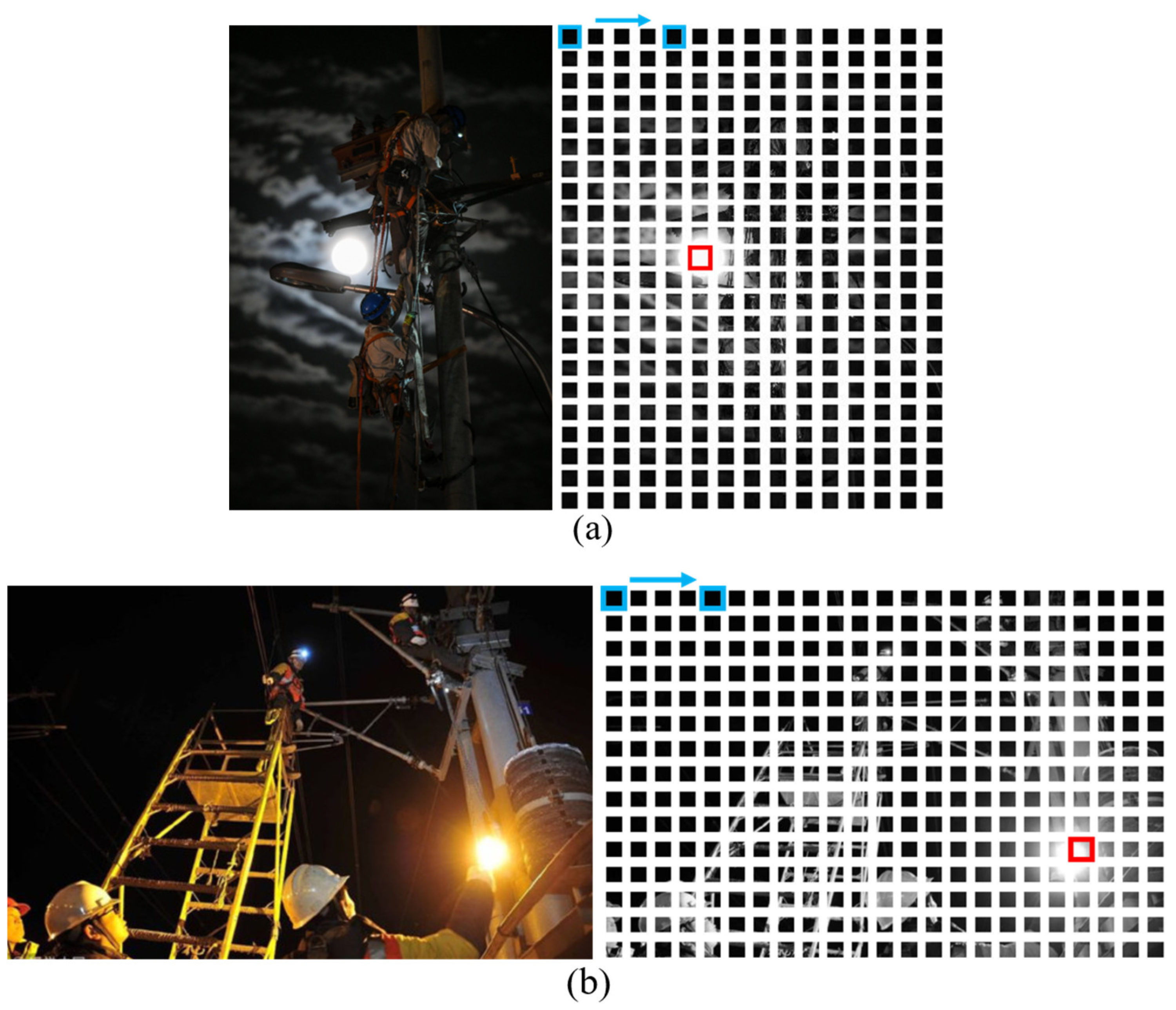
The low-light RGB input image is first converted to grayscale and then 1/15 of the grayscale image’s width is used as the side length a of the square sliding window (blue box in Figure 3), which sequentially slides from the upper-left corner in the steps of a. Each pixel point in the subimage has a gray value of x(i,j) (0 ≤ i < a, 0 ≤ j < a), with an x range of 0–255. By calculating the gray-level average of 200 strong light subimages from (1), we could determine the strong light grayscale threshold to be θ = 190.
Finally, the average value of the deviation (AVG) and average deviation (A.D.) is calculated between each subimage and the strong light grayscale threshold (θ), further calculating the brightness parameter S. When S > 1 and AVG > 0, it may be determined that there is strong light in the image (red box in Figure 3).
The calculation formula of the average value of the deviation between the grayscale image and the strong light threshold is:
The average deviation of the grayscale image from the strong light threshold is calculated as:
In the gray map, H[i] is the quantity of pixels of level i of gray. The luminance parameter s is calculated as:
3.2. Light Effect Decomposition Based on Layer Decomposition Network
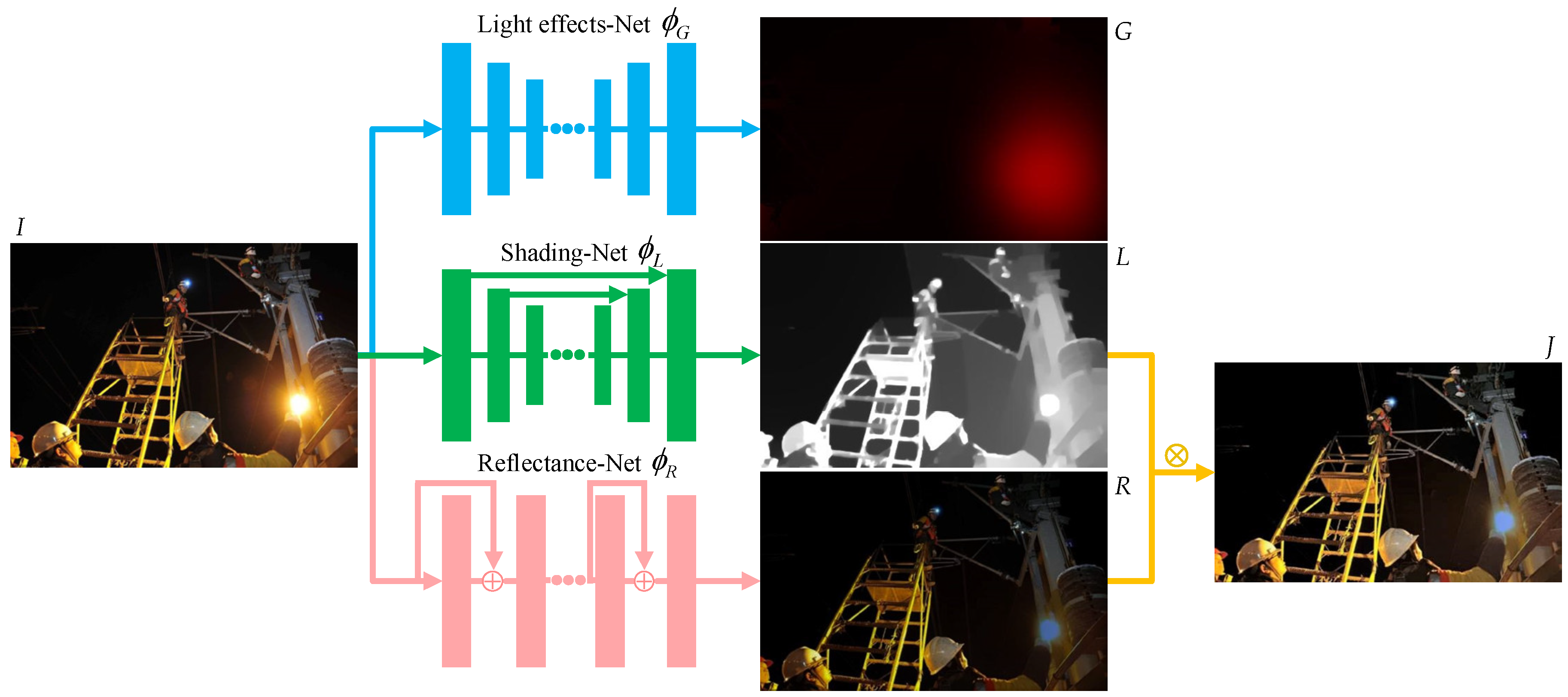
An RGB image judged to be in the presence of strong light is fed into the layer decomposition network [13], which is then decomposed into a light effect layer, a shading layer, and a reflectance layer by means of three independent networks, ϕG, ϕL, and ϕR, and unsupervised loss, as shown in Figure 4. The light effect decomposition results of the RGB image are obtained as follows:
G = ϕG(I) is the light effect layer, L = ϕL(I) is the shading layer, R = ϕR(I) is the reflectance layer, and denotes element-by-element multiplication. In order to achieve the effect of removing the strong light effect, we must first remove the light effect layer G in order to obtain a background layer J = RL that is unaffected by the light effect. Low-light enhancement based on the background layer J reduces the interference of strong light effects.
The layer decomposition network uses a series of unsupervised losses; in the initial phase of training, G and L are supervised using Gi and Li to directly calculate the L1 loss:
where Gi is the smooth map generated by second-order Laplace filtering on the input image and Li is the grayscale map generated by taking the maximum of the three channels at each position of the input image. In addition, the gradient map of G has a short-tailed distribution; i.e., the map of G is smooth with small gradients and almost no large gradients, while the gradient map of J (J = RL) has a long-tailed distribution. With the help of this property, a loss called Gradient Exclusion Loss is used, which makes it possible to separate the G and J layers in the gradient space. The definition of Gradient Exclusion Loss is as follows:
where G↓n and J↓n denote G and J after sampling under bilinear interpolation, the parameters and are normalization factors, and is the Frobenius paradigm number. The Frobenius paradigm is a matrix paradigm defined as follows:
where A* is A’s conjugate transposition and σi represents A’s singular value. The loss of color constancy is set to the following amount in order to reduce color shift in the decomposition output and equalize the range of intensity values of the three-color channels in the background picture J.
where (c1, c2)∈{(r, g), (r, b), (g, b)} represents the combination of two-color channels. For the decomposition task, it is also required that the predicted combination of three layers also recovers the original input image, setting the reconstruction loss as follows:
3.3. Zero-DCE Low-Light Enhancement Network Based on a Kernel Selection Module
The low-light enhancement is disturbed by noise, which loses the local information around the noise, resulting in blurred images. To solve this problem, inspired by SKNet (Selective Kernel Networks) [15], we propose a Zero-DCE low-light enhancement network based on a kernel selection module. The low-light image is taken as the input, the curve parameter maps are learned using DCE-KSNet (Deep Curve Estimation Network Based on a Kernel Selection Module), and then the low-light image is adjusted at the pixel level by the luminance enhancement curves. An enhanced image is obtained after several iterations. The network framework is shown in Figure 5.
The luminance enhancement curve is:
where An signifies the curve parameter map with a size equal to the input image, x denotes the image pixel coordinates, and n denotes the number of iterations. After the above equation, each pixel of the input image is endowed with an optimal higher-order curve that enables it to dynamically adjust its brightness.
DWConv (depthwise separable convolution) [16] is used in place of a regular convolution in DCE-Net (Deep Curve Estimation Network) in order to decrease the number of parameters and computing effort. The deep convolution block separately convolves each channel to extract the data for a single channel and then extends or compresses the input feature maps’ channels by a 1 × 1 point-by-point convolution block to produce feature maps of the desired size. The deep separable convolution kernel can drastically reduce the number of parameters in the network compared with a regular convolution kernel while essentially maintaining network accuracy. Noise interference can be reduced by fully utilizing spatial features and using different scales of receptive fields for multi-scale fusion. In terms of multi-scale feature fusion, most of the existing methods are based on a feature pyramid structure, combining features by way of an element addition or a series connection, which ignores the spatial and channel specificities of the features of different scales, although it can combine feature maps of different scales. A three-branch kernel selection module is added, as shown in Figure 5, after the 7th convolutional layer of DCE-Net to adaptively adjust the receptive field size, dynamically select the appropriate path, and reduce the impact of noise on the low-light enhancement.
Convolution kernels of sizes 3, 5, and 7 are used to process the input feature map U to produce the output feature maps U’, U″, and U‴, with the 5 × 5 convolution kernel being made up of two 3 × 3 dilated convolutions. The three are then added to produce to integrate the data from all branches. is embedded into the global information s by GAP (Global Average Pooling).
The dimensions of the feature map are H and W; s is then passed through the fully connected layer to produce a compact feature map z ∈ Rd×C:
where B is the batch normalization process, δ is the RELU activation function, and W ∈ Rd×C and d values are controlled by the compression ratio r:
where L is the minimum value of d, generally taken as L = 32.
In order to obtain weights at different spatial scales and, thus, the weighted fusion information for different sensory fields, a Softmax operation in the direction of the vector z-channel is obtained:
where A, B, C ∈ RC×d, and Ac ∈ R1×d denote the cth row of A, αc is the cth element of α, and α is the weight vector of U’. Finally, the feature maps processed by different-sized convolutional kernels are multiplied with their corresponding weight vectors to obtain the final output feature maps:
where V = [V1, V2, …, Vc] and Vc ∈ RH×W.
In order to enable the network to complete training with zero reference information, a series of non-reference losses is employed, including spatial consistency loss, exposure control loss, color constancy loss, and luminance smoothing loss.
- (1)
- Spatial Consistency Loss
To prevent a significant change in the value of a pixel’s adjacent pixels between the original image and the enhanced version, the error Lspa is set as follows:
where K is the number of localized regions and Ω(i) is the four adjacent domains (up, down, left, and right) centered on region i. As seen in Figure 6, we set the size of the localized regions to 4 × 4; I and Y are the average intensity values of the localized regions in the input low-light image and the enhanced image, respectively.
- (2)
- Exposure Control Loss
The exposure control loss indicates the distance between the average intensity value and the ideal exposure value E so that the image is enhanced with a good exposure value with the following equation:
where Y represents the local region’s average intensity value in the enhanced image; E is the ideal RGB color space’s gray level [17,18], which is set to 0.6 [12]; and M is the number of 16 × 16 non-overlapping regions.
- (3)
- Color Constancy Loss
According to the gray world color constancy assumption [19], each sensor channel’s color is averaged over the entire image and the loss of color constancy is used to correct any potential color deviations in the enhanced image. An adjustment relationship is established between the three RGB channels to ensure that their average values are as similar as possible to their average values after the enhancement of the image.
where and denote the average intensity values of channels p and q, respectively, and (p, q) denotes the set of channels belonging to ε.
- (4)
- Luminance Smoothing Loss
To maintain a monotonic relationship between surrounding pixels or to lessen the impact of brightness changes between adjacent pixels, a lighting smoothing loss is added to each curve parameter mapping.
where N denotes the number of iterations, denotes the curve parameter map of each channel, denotes the horizontal gradient of the image, denotes the vertical gradient of the image, and ξ denotes the RGB three-channel color.
The total network loss is the sum of the above four losses.
where W1, W2, W3, and W4 are the weight values of the four losses, which are 1, 10, 5, and 1600, respectively [12].
4. Experiments
On different datasets, we ran comparison experiments with state-of-the-art methods.
4.1. Datasets
The SICE [20] Part 1 public dataset contains 2002 images with different exposures and the SCIE Part 2 dataset contains 229 sets of labeled images with different exposures; the private dataset of the electric power operation site is 500 images with different exposures, provided by Baishan City Power Supply Company of State Grid Jilin Electric Power Co. (Baishan City, China).
4.2. Environment Configuration
The experiments were performed on a server consisting of an Ubuntu version 18.04 operating system with a Linux kernel, Python 3.7, PyTorch 1.8.1+cu101, and an NVIDIA Tesla T4 GPU (NVIDIA, Santa Clara, CA, USA).
4.3. Training and Testing
The Zero-DCE low-light enhancement network based on the a kernel selection module was trained using the SCIE Part 1 dataset and the power job site private dataset, with a learning rate of 0.001 and a total training epoch of 100. It was tested on the power job site private dataset as well as the SICE Part 2 dataset.
4.4. Evaluation
For the private dataset of the electric power operation site without labeling, the subjective visual effect and the number of human keypoints correctly detected by HRNet (High-Resolution Net) [21] estimation model were used as the evaluation metrics for the superiority of the image enhancement effect. For the labeled SCIE public dataset images, PSNR (peak signal-to-noise ratio) and SSIM [22] (structural similarity) were used as the evaluation metrics, which were calculated using MATLAB built-in functions.
When comparing the quality of a low-light augmented image to a true labeled image, the PSNR, an engineering term that describes the ratio of the highest achievable strength of a signal to the power of the destructive noise that influences its representation accuracy, was utilized. The definition of PSNR for an original image I of size m × n and a processed image K is:
where the MSE (mean square error) is:
MAXI indicates the maximum value of the image point color. Each pixel has a value of 255 when it is represented in 8-bit binary and 2B − 1 when it is represented in B-bit binary. The higher the PSNR, the less distortion there is and the closer it is to the original image.
SSIM is a metric used to compare two pictures. Two images—the real labeled image and the low-light enhanced image—were used to calculate the SSIM. The two photos’ SSIMs were calculated as follows:
where μx is the mean value of x, is the variance of x, y is the same, is the covariance of x and y, c1 = (k1L)2 and c2 = (k2L)2 are constants used to maintain stability, and L is the dynamic range of the pixel values. k1 = 0.01 and k2 = 0.03. The structural similarity had a range from 0 to 1 and the value of the SSIM was equal to 1 when the two images were exactly alike.
In order to evaluate the light weight of the model, the number of parameters (Params) and the number of floating-point operations (FLOPs) in the network were used as evaluation metrics.
4.5. Results
4.5.1. Luminance Enhancement Curve Effectiveness Experiment
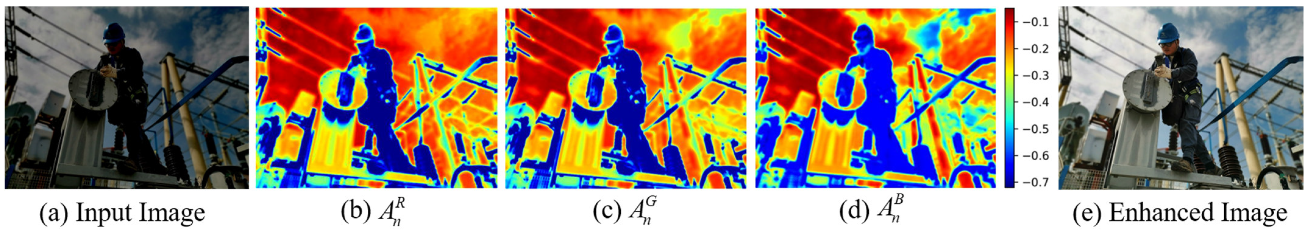
Figure 7 shows an example of the curve parameter plot An for the three RGB channels, demonstrating the validity of the luminance enhancement curve (Equation (11)). For visualization, we averaged the curve parameter plots over eight iterations and normalized the values to the range [0, 1]. The average best-fit curve parameter plots for the R, G, and B channels were denoted by the letters , , and , respectively. Heat maps were used to visualize the mappings, as shown in Figure 7 images (b), (c), and (d). There were correlations and differences between the three channels of the low-light image, as seen by the best-fit parameter maps for the various channels, which had similar tuning trends but with distinct values. It can be seen that for any of the RGB channels, the enhancement values were smaller in the bright regions and larger in the dark regions.
4.5.2. Ablation Experiment of Each Loss
To demonstrate the effectiveness of the four losses, we conducted ablation experiments. The low-light enhancement effects are shown in Figure 8, where (a) is the input low-light image; (b) is the low-light enhancement result, including four kinds of losses, where the brightness and color have reached the ideal effect; (c) is the result of removing the spatial consistency loss (Lspa) and the image contrast is significantly reduced, such as part of the character’s clothes; (d) is the result of removing exposure control loss (Lexp), where the low-light area of the image has not been enhanced and is still dark; (e) is the result of removing color constancy loss (Lcol), where the image has obvious color loss and the overall color turns green; and (f) is the result of removing luminance smoothing loss (LtvA), where the image has obvious artifacts, seriously affecting the visual effect. Through the ablation experiments of each loss, it can be seen that the four different losses had different contributions to low-light enhancement; removing any one made the low-light enhancement effect worse.
In order to prove the effectiveness of Lspa more objectively, the input original image, the image enhanced by including the four losses, and the image enhanced by removing Lspa were converted to double type and a mesh map luminance visualization was carried out using MATLAB. As shown in Figure 9, image (b) with Lspa included had a roughly similar luminance structure to the input original image (a), while image (c) with Lspa removed had a high overall luminance and a reduced contrast, which further demonstrated the importance of Lspa in preserving the differences in the neighboring regions between the input image and the enhanced image.
4.5.3. Low-Light Enhancement Effect Comparison Experiment
Comparative experiments with other state-of-the-art methods were performed on the SICE Part 2 public dataset and a private dataset of electric power job sites, respectively, to show the efficacy of our low-light enhancement method. Other state-of-the-art methods were selected as UNIE [13], EnlightenGAN [10], LMSPES [9], and Zero-DCE [12]. As the private dataset of the electric power operation site had no labels corresponding with the original image, it could not be judged by objective PSNR and SSIM indexes so the subjective visual effect and the number of correctly detected keypoints were used as the evaluation indexes. In terms of keypoint detection, we used Faster-RCNN [23] as a human detector and HRNet for keypoint detection. The comparison results are shown in Figure 10 and Figure 11, demonstrating the subjective visual enhancement effect and the number of keypoints correctly detected; thus, this paper’s method was superior to other state-of-the-art methods.
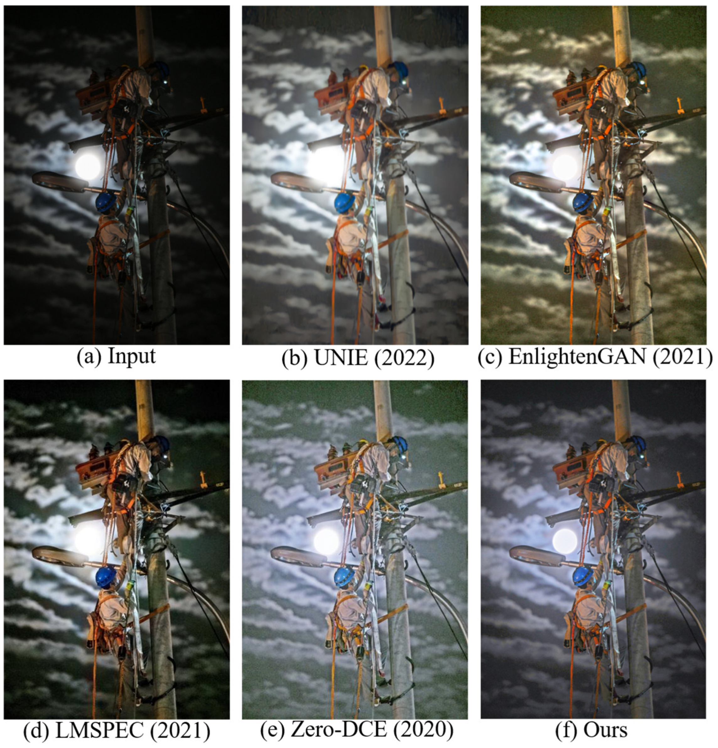
Figure 12 and Figure 13 show a comparison experiment of the image enhancement of a low-light scene of an electric power operation with localized strong light. Our approach was superior to existing approaches in that it improved low-light images while preventing overexposure to strong light. It also provided better overall image visualization and noise control.
Image visualization is subjective, so we also used PSNR and SSIM as evaluation metrics and conducted comparison experiments using the SICE Part 2 public dataset. The metrics were calculated using MATLAB for the images enhanced by different methods and labeled images, respectively. PSNR and SSIM were taken as the average of 100 images. Figure 14 shows the visualization comparison with other advanced methods after low-light enhancement and Table 1 displays the findings from a comparison of PSNR and SSIM.
4.5.4. Model Complexity Comparison Experiment
In order to lighten the network, we used depth-separable convolution to replace the ordinary convolution. The Params and FLOPs of the Zero-DCE low-light enhancement network based on the a kernel selection module (excluding the strong light judgment method and the light effect decomposition method) were substantially reduced compared with the original Zero-DCE. As shown in Figure 15, the Params were about 65% of the original and FLOPs were about 60% of the original when the input image size was 1200 × 900 × 3.
5. Conclusions
This paper proposes a low-light image enhancement method for an electric power operation site considering strong light suppression. Firstly, a sliding-window-based strong light judgment method was designed, then a light effect decomposition method based on a layer decomposition network was used. Finally, a Zero-DCE low-light enhancement network based on a kernel selection module was constructed. Through the joint training of the private and public datasets of the electric power operation site, the visual effect and the number of correctly detected keypoints of the human skeleton were identified. PSNR and SSIM were used as the evaluation indexes for the comparative experiments. The method proposed in this paper outperformed the other state-of-the-art low-light enhancement methods in all the evaluation indexes, which effectively improved the image quality of the low-light environment of the electric power operation site.
Author Contributions
Writing—original draft, Z.Z.; validation, Y.X.; writing—review and editing, Z.Z. and Y.X.; data curation, W.W.; funding acquisition, Y.X. All authors have read and agreed to the published version of the manuscript.
Funding
This work was financially supported by the Jilin Scientific and Technological Development Program (grant number: 20220203135SF).
Institutional Review Board Statement
Not applicable.
Informed Consent Statement
Not applicable.
Data Availability Statement
The SCIE dataset used in this study can be obtained from https://github.com/csjcai/SICE (accessed on 1 June 2023). The private dataset of the power operation site is not available due to further research.
Conflicts of Interest
The authors declare no conflict of interest.
References
- Zhang, F.; Shao, Y.; Sun, Y.; Zhu, K.; Gao, C.; Sang, N. Unsupervised low-light image enhancement via histogram equalization prior. arXiv 2021, arXiv:2112.01766. [Google Scholar]
- Jeong, I.; Lee, C. An optimization-based approach to gamma correction parameter estimation for low-light image enhancement. Multimed. Tools Appl. 2021, 80, 18027–18042. [Google Scholar] [CrossRef]
- Liu, S.; Long, W.; He, L.; Li, Y.; Ding, W. Retinex-based fast algorithm for low-light image enhancement. Entropy 2021, 23, 746. [Google Scholar] [CrossRef] [PubMed]
- Ismail, M.K.; Al-Ameen, Z. Adapted single scale Retinex algorithm for nighttime image enhancement. AL-Rafidain J. Comput. Sci. Math. 2022, 16, 59–69. [Google Scholar] [CrossRef]
- Ma, L.; Lin, J.; Shang, J.; Zhong, W.; Fan, X.; Luo, Z.; Liu, R. Learning multi-scale retinex with residual network for low-light image enhancement. In Proceedings of the Chinese Conference on Pattern Recognition and Computer Vision, Nanjing, China, 16–18 October 2020; pp. 291–302. [Google Scholar]
- Wang, F.; Zhang, B.; Zhang, C.; Yan, W.; Zhao, Z.; Wang, M. Low-light image joint enhancement optimization algorithm based on frame accumulation and multi-scale Retinex. Ad Hoc Netw. 2021, 113, 102398. [Google Scholar] [CrossRef]
- Lore, K.G.; Akintayo, A.; Sarkar, S. LLNet: A deep autoencoder approach to natural low-light image enhancement. Pattern Recognit. 2017, 61, 650–662. [Google Scholar] [CrossRef]
- Wei, C.; Wang, W.; Yang, W.; Liu, J. Deep retinex decomposition for low-light enhancement. arXiv 2018, arXiv:1808.04560. [Google Scholar]
- Afifi, M.; Derpanis, K.G.; Ommer, B.; Brown, M.S. Learning multi-scale photo exposure correction. In Proceedings of the IEEE/CVF Conference on Computer Vision and Pattern Recognition, Nashville, TN, USA, 20–25 June 2021; pp. 9157–9167. [Google Scholar]
- Jiang, Y.; Gong, X.; Liu, D.; Cheng, Y.; Fang, C.; Shen, X.; Yang, J.; Zhou, P.; Wang, Z. Enlightengan: Deep light enhancement without paired supervision. IEEE Trans. Image Process. 2021, 30, 2340–2349. [Google Scholar] [CrossRef] [PubMed]
- Ronneberger, O.; Fischer, P.; Brox, T. U-net: Convolutional networks for biomedical image segmentation. In Proceedings of the Medical Image Computing and Computer-Assisted Intervention, Part III 18, Munich, Germany, 5–9 October 2015; pp. 234–241. [Google Scholar]
- Guo, C.; Li, C.; Guo, J.; Loy, C.C.; Hou, J.; Kwong, S.; Cong, R. Zero-reference deep curve estimation for low-light image enhancement. In Proceedings of the IEEE/CVF Conference on Computer Vision and Pattern Recognition, Seattle, WA, USA, 13–19 June 2020; pp. 1780–1789. [Google Scholar]
- Jin, Y.; Yang, W.; Tan, R.T. Unsupervised night image enhancement: When layer decomposition meets light-effects suppression. In Proceedings of the European Conference on Computer Vision, Tel Aviv, Israel, 23–27 October 2022; pp. 404–421. [Google Scholar]
- Radulescu, V.M.; Maican, C.A. Algorithm for image processing using a frequency separation method. In Proceedings of the 2022 23rd International Carpathian Control Conference (ICCC), Sinaia, Romania, 29 May–1 June 2022; pp. 181–185. [Google Scholar]
- Li, X.; Wang, W.; Hu, X.; Yang, J. Selective kernel networks. In Proceedings of the IEEE/CVF Conference on Computer Vision and Pattern Recognition, Long Beach, CA, USA, 15–20 June 2019; pp. 510–519. [Google Scholar]
- Chollet, F. Xception: Deep learning with depthwise separable convolutions. In Proceedings of the IEEE Conference on Computer Vision and Pattern Recognition, Honolulu, HI, USA, 21–26 July 2017; pp. 1251–1258. [Google Scholar]
- Mertens, T.; Kautz, J.; Van Reeth, F. Exposure fusion. In Proceedings of the 15th Pacific Conference on Computer Graphics and Applications (PG’07), Maui, HI, USA, 29 October–2 November 2007; IEEE: Piscataway, NJ, USA, 2007; pp. 382–390. [Google Scholar]
- Mertens, T.; Kautz, J.; Van Reeth, F. Exposure fusion: A simple and practical alternative to high dynamic range photography. Comput. Graph. Forum 2009, 28, 161–171. [Google Scholar] [CrossRef]
- Buchsbaum, G. A spatial processor model for object colour perception. J. Frankl. Inst. 1980, 310, 1–26. [Google Scholar]
- Cai, J.; Gu, S.; Zhang, L. Learning a deep single image contrast enhancer from multi-exposure images. IEEE Trans. Image Process. 2018, 27, 2049–2062. [Google Scholar]
- Wang, J.; Sun, K.; Cheng, T.; Jiang, B.; Deng, C.; Zhao, Y.; Liu, D.; Mu, Y.; Tan, M.; Wang, X.; et al. Deep high-resolution representation learning for visual recognition. IEEE Trans. Pattern Anal. Mach. Intell. 2020, 43, 3349–3364. [Google Scholar] [CrossRef]
- Wang, Z.; Bovik, A.C.; Sheikh, H.R.; Simoncelli, E.P. Image quality assessment: From error visibility to structural similarity. IEEE Trans. Image Process. 2004, 13, 600–612. [Google Scholar] [CrossRef] [PubMed]
- Ren, S.; He, K.; Girshick, R.; Sun, J. Faster R-CNN: Towards Real-Time Object Detection with Region Proposal Networks. arXiv 2015, arXiv:1506.01497. [Google Scholar] [CrossRef]
Figure 1.
Comparison between low-light and normal images. (a,b,d) is a low-light image, where (d) contains local strong lighting. (c) is the normal-illuminated image.
Figure 1.
Comparison between low-light and normal images. (a,b,d) is a low-light image, where (d) contains local strong lighting. (c) is the normal-illuminated image.

Figure 2.
Flowchart of low-light image enhancement method for electric power operation sites.

Figure 3.
Strong light search based on a sliding window. (a,b) are examples of two sets of strong light search based on a sliding window, respectively. The blue boxes are sliding windows with a step size of 1 and S-shaped search. The red boxes are the searched strong light.
Figure 3.
Strong light search based on a sliding window. (a,b) are examples of two sets of strong light search based on a sliding window, respectively. The blue boxes are sliding windows with a step size of 1 and S-shaped search. The red boxes are the searched strong light.

Figure 4.
Light effect decomposition based on layer decomposition network. I is the input image, G is the light effect layer, L is the shading layer, R is the reflectance layer, and J is the background layer.
Figure 4.
Light effect decomposition based on layer decomposition network. I is the input image, G is the light effect layer, L is the shading layer, R is the reflectance layer, and J is the background layer.

Figure 5.
Zero-DCE low-light enhancement network framework based on a kernel selection module.

Figure 6.
Example of spatial consistency loss. The red squares are the central pixel, and the green squares are the four adjacent pixels.
Figure 6.
Example of spatial consistency loss. The red squares are the central pixel, and the green squares are the four adjacent pixels.

Figure 7.
RGB channel curve parameter graph.

Figure 8.
Ablation experiment of each loss.

Figure 9.
Comparison of Lspa effectiveness using mesh charts. The red boxes are two obvious and representative contrast differences.
Figure 9.
Comparison of Lspa effectiveness using mesh charts. The red boxes are two obvious and representative contrast differences.

Figure 10.
The first group of comparison experiments of low-light enhancement and keypoint detection in electric power operation site. The red font is the best result of keypoint detection.
Figure 10.
The first group of comparison experiments of low-light enhancement and keypoint detection in electric power operation site. The red font is the best result of keypoint detection.

Figure 11.
The second group of comparison experiments of low-light enhancement and keypoint detection in electric power operation site. The red font is the best result of keypoint detection.
Figure 11.
The second group of comparison experiments of low-light enhancement and keypoint detection in electric power operation site. The red font is the best result of keypoint detection.

Figure 12.
The first group of comparative experiments of low-light enhancement at an electric power operation site in the presence of strong light.
Figure 12.
The first group of comparative experiments of low-light enhancement at an electric power operation site in the presence of strong light.

Figure 13.
The second group of comparative experiments of low-light enhancement at an electric power operation site in the presence of strong light.
Figure 13.
The second group of comparative experiments of low-light enhancement at an electric power operation site in the presence of strong light.

Figure 14.
Comparison of portions of the Part 2 testing dataset.

Figure 15.
Comparison of Params and FLOPs.


Disclaimer/Publisher’s Note: The statements, opinions and data contained in all publications are solely those of the individual author(s) and contributor(s) and not of MDPI and/or the editor(s). MDPI and/or the editor(s) disclaim responsibility for any injury to people or property resulting from any ideas, methods, instructions or products referred to in the content. |
© 2023 by the authors. Licensee MDPI, Basel, Switzerland. This article is an open access article distributed under the terms and conditions of the Creative Commons Attribution (CC BY) license (https://creativecommons.org/licenses/by/4.0/).
Share and Cite
MDPI and ACS Style
Xi, Y.; Zhang, Z.; Wang, W. Low-Light Image Enhancement Method for Electric Power Operation Sites Considering Strong Light Suppression. Appl. Sci. 2023, 13, 9645. https://0-doi-org.brum.beds.ac.uk/10.3390/app13179645
AMA Style
Xi Y, Zhang Z, Wang W. Low-Light Image Enhancement Method for Electric Power Operation Sites Considering Strong Light Suppression. Applied Sciences. 2023; 13(17):9645. https://0-doi-org.brum.beds.ac.uk/10.3390/app13179645
Chicago/Turabian StyleXi, Yang, Zihao Zhang, and Wenjing Wang. 2023. "Low-Light Image Enhancement Method for Electric Power Operation Sites Considering Strong Light Suppression" Applied Sciences 13, no. 17: 9645. https://0-doi-org.brum.beds.ac.uk/10.3390/app13179645
Note that from the first issue of 2016, this journal uses article numbers instead of page numbers. See further details here.