

Detection of Wheat Yellow Rust Disease Severity Based on Improved GhostNetV2

1
College of Information Science and Engineering, Henan University of Technology, Zhengzhou 450001, China
2
Key Laboratory of Grain Information Processing and Control, Henan University of Technology, Zhengzhou 450001, China
*
Author to whom correspondence should be addressed.
Appl. Sci. 2023, 13(17), 9987; https://0-doi-org.brum.beds.ac.uk/10.3390/app13179987
Submission received: 4 June 2023
/
Revised: 1 July 2023
/
Accepted: 10 July 2023
/
Published: 4 September 2023
(This article belongs to the Topic Applied Computer Vision and Pattern Recognition: 2nd Volume)
Abstract
:Wheat production safety is facing serious challenges because wheat yellow rust is a worldwide disease. Wheat yellow rust may have no obvious external manifestations in the early stage, and it is difficult to detect whether it is infected, but in the middle and late stages of onset, the symptoms of the disease are obvious, though the severity is difficult to distinguish. A traditional deep learning network model has a large number of parameters, a large amount of calculation, a long time for model training, and high resource consumption, making it difficult to transplant to mobile and edge terminals. To address the above issues, this study proposes an optimized GhostNetV2 approach. First, to increase communication between groups, a channel rearrangement operation is performed on the output of the Ghost module. Then, the first five G-bneck layers of the source model GhostNetV2 are replaced with Fused-MBConv to accelerate model training. Finally, to further improve the model’s identification of diseases, the source attention mechanism SE is replaced by ECA. After experimental comparison, the improved algorithm shortens the training time by 37.49%, and the accuracy rate reaches 95.44%, which is 2.24% higher than the GhostNetV2 algorithm. The detection accuracy and speed have major improvements compared with other lightweight model algorithms.
1. Introduction
Wheat is a worldwide high-economic crop with rich nutritional value and is one of the important sources of food and industrial raw materials for human beings. Diseases have a great impact on the yield and quality of wheat, and yellow rust is a very harmful disease. Wheat yellow rust is a disease caused by fungi, which has a high incidence and rapid spread under suitable temperatures and moisture and poses a serious threat to wheat yield. The characteristics of emerging yellow rust are similar to the characteristics of natural or mechanical damage to leaves. If it is misjudged as disease-free and the disease is allowed to continue to infect, the wheat yield will inevitably decline. However, farmers usually judge the degree of damage based on the size of the diseased area on the leaves, but this method is prone to misjudgment, resulting in the excessive use of pesticides or failure to achieve the level of pest control, which will reduce crop production and cause economic losses. Thus, the timely and accurate judgment of wheat yellow rust and the degree of damage is an urgent problem to be solved [1,2,3,4,5].
The assessment of the severity of wheat diseases is of great significance for preventing and controlling the spread of diseases and improving the yield and quality of wheat [6]. The assessment of traditional wheat disease severity mainly relies on manual diagnosis, which is not just time-consuming and labor-intensive but also subjective and error-prone. Currently, the most professional detection of agricultural diseases is based on biochemical tests, of which polymerase chain reaction (PCR) is commonly used [7]. However, using remote sensing technologies, such as hyperspectral, multispectral, or RGB images, combined with machine learning and other methods to realize automatic, accurate, and rapid assessment of wheat disease severity, is a current research hotspot and development trend.
The method based on hyperspectral and multispectral images uses the reflectance characteristics of plant leaves in different bands, combined with regression models such as partial least squares regression (PLSR), support vector regression (SVR), and Gaussian process regression (GPR) to estimate disease severity on wheat leaves or canopy. Yuan et al. [8] proposed a monitoring method for wheat leaf rust based on hyperspectral reflectance. Zhang et al. [9] introduced a spectral feature extraction method based on continuous wavelet analysis (CWA) to detect the severity of wheat yellow rust. Compared with traditional spectral features, this method has higher accuracy and speed. Ashourloo et al. [10] compared the performance of three regression models in detecting wheat leaf rust. Shi et al. [11] proposed a method for detecting wheat diseases and insect pests using hyperspectral data and machine learning methods, which have high accuracy and robustness and are superior to traditional methods. Khan et al. [12] introduced a detection method for wheat powdery mildew based on hyperspectral imaging and machine learning. Mustafa et al. [13] used continuous wavelet transform and random forest recursive feature elimination to select consistent spectral bands and developed a canopy-based difference index to differentiate healthy and infected wheat canopies and an estimation of head blight severity. Guan et al. [14] proposed a multi-scale spectral index (SI)-based monitoring method for peanut leaf spot disease, using hyperspectral data to construct and screen SI related to leaf spot disease and using machine learning classifiers to evaluate its detection capabilities. The method has high accuracy and stability at different scales. Mustafa [15] et al. proposed a detection method for wheat head blight based on chlorophyll-related phenotypes and machine learning, using hyperspectral reflectance, chlorophyll fluorescence imaging, and biochemical parameters to extract features related to head blight, and using a feature selection algorithm and multivariate k-nearest neighbor model to detect and classify head blight. This method can detect scabs at an early stage and help control the spread of the pathogen and optimize fungicide application.
The method based on RGB images uses the color characteristics of plant leaves or ears in the visible light range, combined with deep learning and other methods, to identify and classify different types or severity of diseases. Liu et al. [16] developed a new red-edge head blight index (REHBI) to detect and evaluate the severity of FHB in wheat canopies at a regional scale. Schirrmann et al. [17] used a large annotation database taken by a standard RGB camera to detect and classify stripe rust on wheat leaves, using the U2Net model and the deep residual neural network (ResNet) model to achieve 90% accuracy. Hayit et al. [18] proposed a computer model for detecting and classifying wheat yellow rust, named Yellow-Rust-Xception, which can judge whether wheat has yellow rust according to the structural changes in wheat leaf images and how bad the yellow rust is, and obtained a high accuracy rate. In addition, some researchers have utilized segmentation techniques to assess disease severity. Deng et al. [19] proposed a deep-learning-based semantic segmentation method for segmenting stripe rust regions on wheat leaves and automatically calculated the macroscopic disease index (MDI) for measuring canopy disease incidence. Gao et al. [20] proposed a method based on an automatic serial double BlendMask network for segmenting wheat ear and head blight area, and divided head blight into four grades according to the ratio of lesion area to the total area. Mao et al. [21] proposed a deep-neural-network-based scab diagnostic system capable of identifying and localizing four infection levels and generating descriptive phrases.
Hyperspectral and multispectral technologies have the advantages of high precision and high resolution in agricultural disease detection, but they still have shortcomings, such as high costs and difficult data processing and analysis. Conventional deep learning networks may face disadvantages, such as high model complexity, long training times, high hardware resources, and energy consumption, in agricultural disease identification. A lightweight convolutional neural network can reduce the amount of calculation and memory usage required by the model while ensuring the recognition accuracy by weighing factors, such as model parameters and computational complexity, and realizing efficient disease identification and classification on the mobile terminal. There are advantages to real-time mobile applications. The mobile terminal has become more and more mature. The mobile terminal uses image processing technology and deep learning methods to conveniently and precisely identify crop diseases, assess the severity of diseases and track disease progress, and provide effective prevention and control suggestions while reducing production costs, protecting the environment, and improving the market competitiveness of agricultural products. Additionally, through a lightweight convolutional neural network model to achieve a balance between recognition accuracy, computing speed, and network size, it can quickly and cheaply disseminate information to other people in remote areas and strengthen contact with human experts. Therefore, the identification of agricultural diseases on the mobile side of the lightweight network is a worthy study.
The severity of wheat yellow rust is difficult to automatically detect, and the traditional deep learning network consumes a lot of money, which is not suitable for mobile and edge terminals. In response to these problems, this study proposes a lightweight model based on the improved GhostNetV2 to detect the severity of wheat yellow rust. The contributions of this study are as follows:
- (1)
- A channel shuffling operation is added to the Ghost module to strengthen the information flow between group feature maps and enhance the model learning ability.
- (2)
- The shallow layer of the model is replaced with the Fused-MBConv module, the training time of the model is reduced by 37.49%, and the training efficiency of the model is improved.
- (3)
- The SE of the model is replaced with the ECA to further improve the focus of the model on the disease and reduce the parameters of the model.
2. Materials and Methods
2.1. Image Dataset
The data in this article come from Yellow-Rust-19 [22]. It is formed from scratch after a series of operations including planting, inoculation and incubation, leaf image acquisition, labeling, and image processing. The data set has a total of 4995 images. During the image acquisition process, environmental conditions such as weather, light, and temperature were considered. There are 6 grades of yellow rust, which are disease-free (0), resistant (R), moderately resistant (MR), moderately resistant–moderately susceptible (MRMS), moderately susceptible (MS), and susceptible (S). Figure 1 depicts these severity levels and provides some samples for each severity level in the dataset.
2.2. Image Processing
The color of the wheat image acquired in the natural scene of the field will be different from the light intensity of visual perception due to changes, which will impact the effectiveness of CNN for disease feature extraction. In this study, we use the single-scale Retinex [23] algorithm to enhance the images. Its purpose is to separate the illumination and reflection from the image, and then process the reflection to improve the contrast and color restoration of the image. The algorithm is as follows:
Take the logarithm of the image:
where I(x,y) is the brightness of the image, L(x,y) is the illuminance, and R(x,y) is the reflection. Illuminance represents the intensity and direction of the light source, and reflection represents the inherent properties of the object.
Perform Gaussian filtering on the image to obtain an approximation of the illuminance:
Among them, G(x,y) is a Gaussian kernel function and ∗ represents a convolution operation.
Subtract an approximation of the illuminance from the image to obtain the logarithm of the reflection:
Gray-scale stretching is performed on the logarithm of the reflection to obtain an enhanced reflection:
Multiply the enhanced reflection with the original illuminance to obtain the enhanced image:
2.3. Methods
2.3.1. Model Introduction
With the development of the times, mobile devices have become the main tool used by people. However, large-scale deep learning network models have many parameters and high computing requirements, making it difficult to transplant to mobile terminals. The emergence of lightweight network models solves this problem very well. Compared with large-scale deep network models, lightweight network models have very few parameters and calculations, and the model performance is not inferior to large-scale deep network models and can adapt to scenarios with limited hardware resources, such as mobile terminals and embedded devices. Currently, two types of lightweight networks are commonly used for model compression and compact model design. Knowledge distillation, network pruning, quantization, low-rank decomposition, etc., are commonly used model compression methods. Compact model design is also a very efficient method. For example, MobileNet [24] uses depthwise separable convolution as the basic unit while maintaining the effect, and the calculation amount and parameter number of the model are greatly reduced. ShuffleNet [25] adopts group shuffling, connects different groups, and fully learns features to ensure complete information. When the network is trained, the output feature maps (as shown in Figure 3) of ordinary convolutions (as shown in Figure 4) usually contain a lot of redundancy, some of which may be similar to each other. The main innovation of the GhostNet [26] network is the introduction of the Ghost module (as shown in Figure 5), which reduces the number of convolution kernels and calculations by using cheap linear transformations to generate redundant feature maps. The Ghost module uses initial convolution and cheap convolution instead of standard convolution. When the network is trained, the input data are X ∈ R(C × H × W) (C, H, W are the number of channels, height, and width), X first passes through the convolution kernel to be 1 × 1 initial convolution:
F1×1 is a pointwise convolution, and Y′ ∈ R (H × W × C′out) is an intrinsic feature. Then, use cheap convolution to generate more features, and connect the features generated by the initial convolution and the features generated by cheap convolution based on the channel, namely:
where Fdp is a depthwise convolutional filter and Y ∈ R(H × W × Cout) is the output feature.
Although the Ghost module reduces computation, its ability to capture spatial information is also reduced. Therefore, GhostnetV2 [27] added an attention mechanism (DFC) based on a fully connected layer, which has lower requirements on hardware, can capture the dependencies between long-distance pixels, and can improve the inference speed. The detailed calculation process of DFC attention is as follows.
Given a feature, Z ∈ R (H × W × C), it can be viewed as an HW label, zi ∈ RC, Z = {z11, z12, …, zHW}. Aggregate features along horizontal and vertical directions, respectively. It can be expressed as:
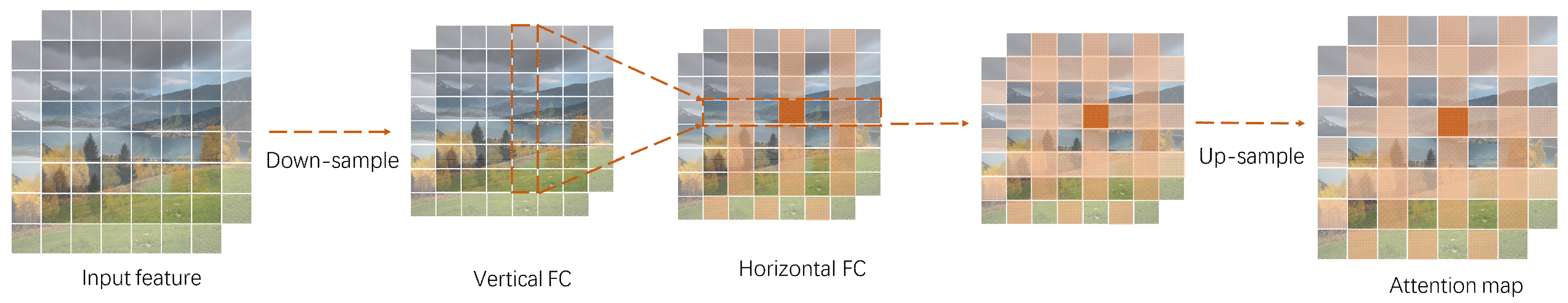
where FH and FW are transformation weights, ⊙ is element-wise multiplication, and A = {a11, a12, …, aHW} is the generated attention map. Taking the original feature Z as input, the long-range dependencies along two directions are captured, and its information flow is shown in Figure 6.
Equations (8) and (9) are representations of DFC attention, which aggregate pixels in two dimensions horizontally and vertically, respectively. To improve inference speed, they exploit partially shared transformation weights and implement them with convolutions, avoiding time-consuming tensor operations. To adapt to input images of different resolutions, they use two depthwise convolutions of size 1 × KH and KW × 1, independent of the feature map size. This method enables fast inference on mobile devices with tools such as TFLite and ONNX, and its theoretical complexity is O(KHHW + KWHW).
Figure 7a,b show the bottleneck structure of GhostNet and GhostNetV2, respectively. On the basis of GhostNet, GhostNetV2 introduces the DFC attention mechanism on the parallel branch of the first Ghost module to enhance the expansion ability of features.
2.3.2. Problems with the Original Model
Although GhostNetV2, which introduces a long-range attention mechanism, has low-cost operation and high performance, the following deficiencies still exist for the wheat yellow rust detection problem that need to be addressed in this study:
- (1)
- The Ghost module generates two sets of feature mappings, where the second set of feature maps is obtained by using linear transformation of the first set of feature maps. Because there are many similar features in the two sets of feature maps and the channel structure is consistent, the model can only learn the main information of one set of feature maps during the training process, while the other set of information is ignored.
- (2)
- Although the original model is a network specially designed for mobile devices, with few model parameters, low calculation, and fast inference speed, the time required for model training is much higher than other lightweight network models.
- (3)
- The similarity of disease severity and the similarity of disease and physical damage make it difficult for the model to identify healthy and diseased wheat and the severity of diseased wheat, so there is a need to improve the model’s detection capability.
2.4. Model Optimization
2.4.1. Optimized Ghost Structure
There are two sets of feature maps in the Ghost module, and the first set of feature maps is generated by ordinary convolution. The second set of feature maps is obtained by performing cheap operations on the first set of feature maps. However, there is no connection between these two groups of feature maps, which leads to insufficient model learning. Therefore, this study proposes the CS-Ghost module (as shown in Figure 8), which performs channel shuffling on the spliced feature maps to strengthen the information flow between the two sets of feature maps. The channel shuffling operation is to scramble the order of the channels of the two sets of feature maps so that each channel can fuse different sets of feature information. Specifically, assuming a set of feature maps has M channels, treat it as a one-dimensional array of (1, M) and reshape it into a two-dimensional array of (g, M/g), where g is the number of groups, take 2; then, transpose the two-dimensional array to obtain an array of (M/g, g); finally, reshape it, restore it to an array of (1, M), and complete the channel shuffling operation. In this way, the CS-Ghost module can make full use of the information from two sets of feature maps and improve the feature expression ability of the model.
2.4.2. Introduce Accelerated FusedMBConv Structure
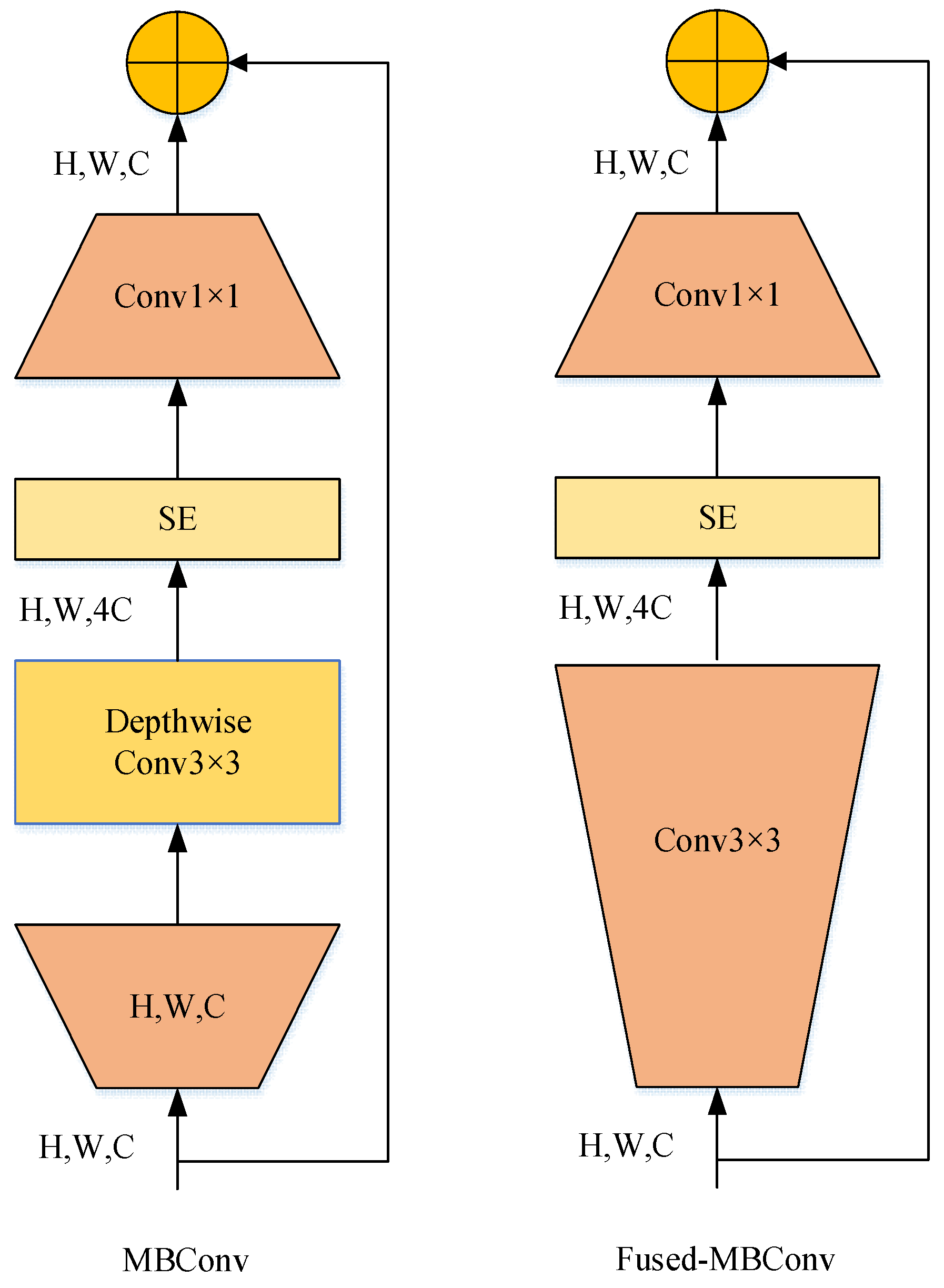
For lightweight networks, most researchers care about model parameters and accuracy. However, the small number of parameters does not mean faster inference speed. EfficientNetv2 [28] focuses on the training speed and inference speed of the model. Compared with deep convolution, ordinary convolution has more parameters and FLOPs, but it can usually take advantage of accelerators and have faster speeds in the shallow layers of the network. To improve the training speed and computational efficiency, EfficientNet introduces the structure of Fused-MBConv. Fused-MBConv replaces the depthwise conv3×3 and expansion conv1×1 in the original MBConv structure with an ordinary conv3×3, as shown in Figure 9. Heavy use of Fused-MBConv in the first few layers of the model speeds up training by a factor of 2.2. Also, Fused-MBConv enhances the expressiveness of the model because it can increase the number of channels without increasing the parameters.
2.4.3. Replace with a More Efficient Attention Module
The attention mechanism is a method to let the deep learning model only focus on the important parts when processing massive amounts of information. It improves the performance and efficiency of the model and also allows the model to better understand the relationship between features and contextual information. There are many forms of attention mechanisms, which are capable of participating in different dimensions and tasks, such as channel, space, self-attention, etc., as well as image recognition, machine translation, picture description, etc.
However, after experiments, it was found that SE [29] in the original model did not pay much attention to the characteristics of wheat yellow rust disease, so we explored an attention mechanism that is more interested in the features of yellow spot disease. ECA [30] (as shown in Figure 10) is an efficient channel attention module, which is characterized by only using one-dimensional convolution to achieve local cross-channel interaction, avoiding dimensionality reduction and global pooling operations, and reducing parameters and calculations. It can adaptively select the size of the convolution kernel, determine the coverage of the interaction, and adapt to feature maps of different scales. It can improve the performance of deep convolutional neural networks while reducing the complexity of the model and has achieved good results in tasks such as image classification, target detection, and instance segmentation. Compared with other channel attention modules, such as SENet, ECA is simpler and more efficient, involving only a small number of parameters and calculations.
2.4.4. Improved Model
This section introduces the improved GhostNetV2 network structure. First, the Ghost module is embedded in the channel shuffle operation to increase network learning communication and improve network performance, and then, the FusedMBConv module is added to the shallow network to reduce model training time. Finally, ECA instead of SE both improves the recognition accuracy of the network model and reduces the network parameters and computational effort. The improved model architecture is shown in Table 1.
2.5. Model Evaluation Index
Accuracy rate, prediction rate, recall rate, F1 score, and confusion matrix are five commonly used evaluation indicators for image classification [31]. The accuracy rate indicates the proportion of correctly classified samples to the total number of samples. The precision rate indicates the proportion of the number of samples predicted to be positive and indeed positive to the number of samples predicted to be positive. The recall rate indicates the proportion of the number of samples that are predicted to be positive and are indeed positive to the number of samples that are indeed positive. The F1 score represents the harmonic mean of precision and recall. The confusion matrix represents the classification between different categories. The horizontal axis is the predicted category, and the vertical axis is the real category. The elements on the diagonal represent the number of samples that are correctly classified, and the elements on the off-diagonal represent the number of samples that are incorrectly classified.
where TP is the true case, TN is the true negative case, P is the total number of positive cases, N is the total number of negative cases, FP is the false positive case, FN is the false negative case.
3. Results
The experimental software and equipment configuration parameters are as follows: Ubuntu 18.04, 64-bit Linux operating system, Tesla T4 graphics card with 16 G memory, pytorch1.7.1, and CUDA10.1.
In the Section 3, three sets of comparative experiments were designed. The first group analyzed the effect of the attention mechanism on the model. The second group was the ablation experiment based on the original GhostNetV2 model. The third group was to compare the improved GhostNetV2 model with the current popular lightweight network model in terms of effect and accuracy.
In this study, we used equal interval adjustment of the learning rate, which is characterized by multiplying the learning rate by a decay factor at every fixed step. It has the advantage that the learning rate can be gradually reduced according to the training process, making the network obtain the optimal solution faster. Weight decay is a method that has been often used to suppress overfitting. This method suppresses overfitting by penalizing large weights during the learning process.
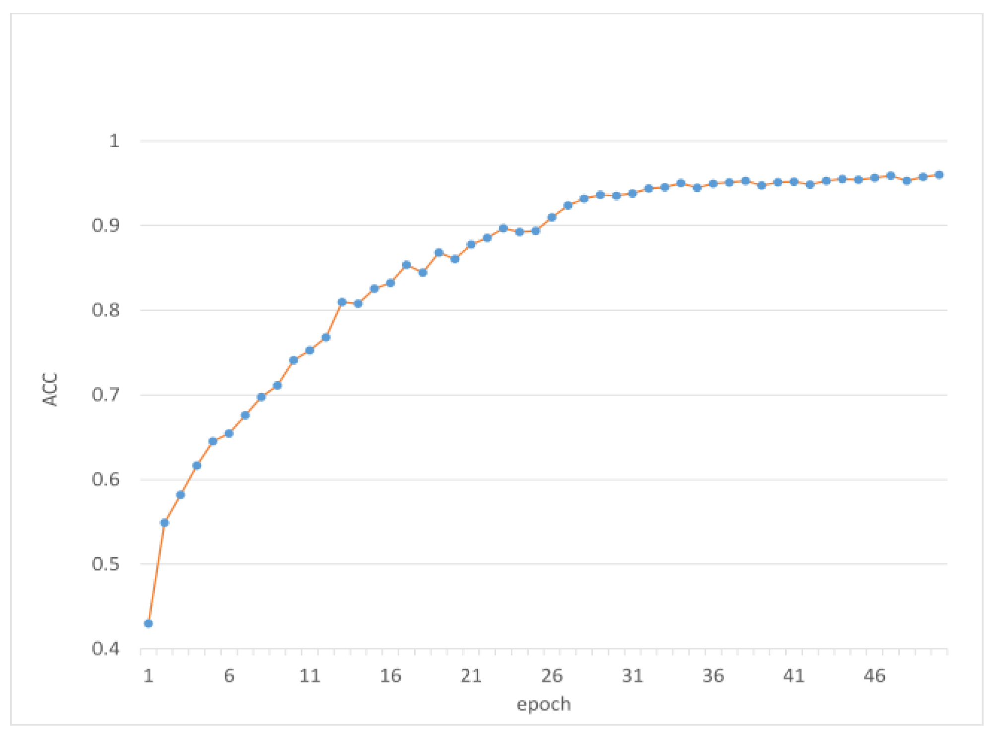
The basic training parameters were as follows: epoch is set to 50; batch size is set to 64; initial learning rate, 0.001; step_size, 25; gamma, 0.01; optimizer, Adam; weight_decay, 0.001; the training is enhanced by random flipping and rotation with a probability of 0.3 data. The change in ACC during training is shown in Figure 11. The training curve is from steep to gentle. When the epoch reaches half, the correct rate increases slowly until the model converges.
3.1. The Impact of Different Attention Mechanisms on the Model
In this study, we tried to replace SE in bottleneck with ECA, CA [32], and CBAM [33], and designed four groups of experiments to test the effects of the four attention mechanisms. Table 2 presents the impact of different attention mechanisms on the model. On the accuracy metric, the ECA model performed best at 0.9496, while the source SE model performed relatively poorly at 0.932. Across the board, the ECA model performed the best of the four, while the source ES model performed the worst. In terms of training time, the ECA model had the shortest training time of 1850 s, while the source SE model had the longest training time of 2847 s. From the perspective of the number of parameters, the source ES model required the most parameters, which was 6.16 M, while the parameters of the other three models were all below 5 M. Therefore, in pursuit of the best indicator performance and the need to consider the training time and model size, the ECA model is a good choice.
In addition, we drew the heat map of the model after the four attention modules using Grad-CAM [34]. Grad-CAM is a visualization method that generates a heat map showing which regions of the input picture are most relevant for the prediction of that category, based on the output category of the network. As shown in Figure 12, CA tended to focus on the edges of the picture, mistaking some backgrounds as part of the disease. SE paid less attention to the characteristics of the disease. CBAM lost most of the disease characteristics and also considered some backgrounds as diseases. ECA paid the highest attention to diseases and could detect almost all disease characteristics. After comparing the four sets of experiments, we replaced the attention mechanism SE in the source model with ECA.
3.2. Effect of Improved Method on Model
Table 3 gives a comparison of the effects of the three improvement methods on the GhostNetV2 model. These methods enhance the effect of the model by using different modules or techniques. The table lists the performance of the four models (GhostNetV2, GhostNetV2_A, GhostNetV2_B, and GhostNetV2_C) obtained using different improvement combinations on the dataset, including the accuracy, F1 score, number of parameters, model calculation amount, inference time, and other indicators. It can be concluded from Table 3 that GhostNetV2_A replaces Ghost in the bottleneck with CS-Ghost. Although the accuracy of the model is increased by 0.36%, it increases the computational cost. To reduce the training time, GhostNetV2_B introduces the FusedMBConv module on the basis of GhostNetV2_A. The training time of the model is significantly shortened, and the accuracy of the model is slightly improved, but the number of parameters of the model is increased by 0.34 M, and the amount of calculation is increased by 0.48 G. Due to the increased computational resources of the model, more memory is required to store the weight parameters. To further improve the performance of the model, GhostNetV2_C introduces the ECA attention mechanism based on GhostNetV2_B. ECA weights the features in the channel dimension through 1D convolution, which is less computationally expensive and more efficient, and allows the network to better analyze disease signatures, thereby improving network performance. GhostNetV2_C reached the highest level in the five indicators of accuracy, F1 score, training time, parameter number, and inference time, which are 95.44%, 95.30%, 1197 s, 5.00 M, and 27.94 ms, of which the training time is reduced by 37.49%.
Figure 13 shows some visualizations of the output feature maps of the improved model and the original model block module. It can be seen from the figure that the improved model extracts brighter image feature information in Block1, such as texture, edge, color, etc. The visual information of the feature map in the deeper Block2 is reduced and the abstract information is increased. In Figure 13b,c, the feature extraction of Block2 in the improved model is very similar to the feature extraction of block in the original model, which proves that our replacement of the model’s shallow CS-Bneck with FusedBMcon does not affect the model’s learning of disease characteristics.
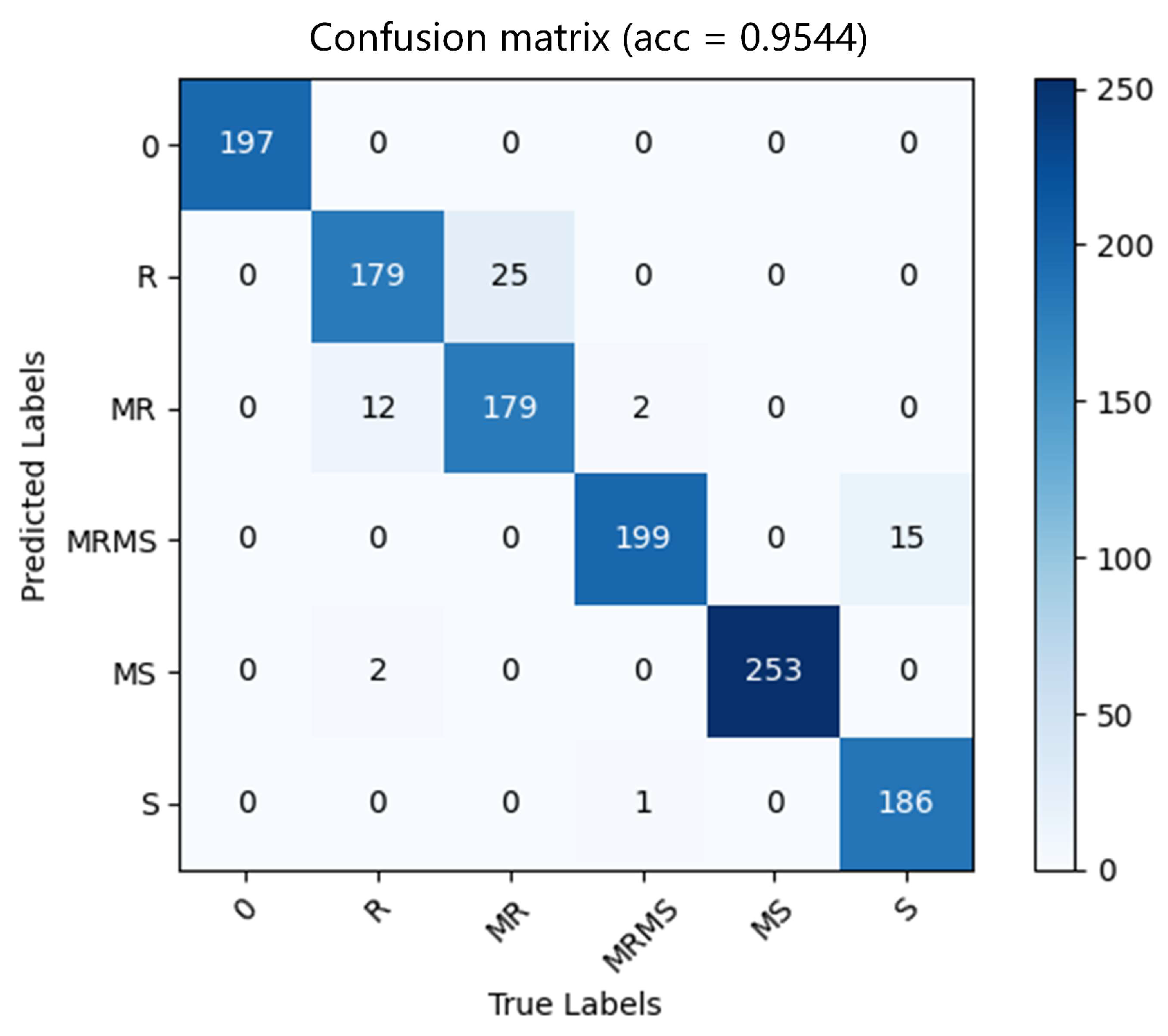
To accurately evaluate the classification effect of the improved model on wheat yellow rust diseases, we drew a confusion matrix based on the test set, as shown in Figure 14, comparing the actual category (abscissa) and the predicted category (ordinate) to show each classification performance of the category. In the figure, 0 indicates healthy wheat, R indicates mild infection, MR indicates medium and small infection, MRMS indicates moderate sensitivity, MS indicates moderate infection, and S indicates severe infection. The diagonal of the confusion matrix represents the number of correct classifications for each category, and the effect is proportional to the value. The larger the value is, the better the effect is. The results show that the improved model has the best recognition effect on moderately infected yellow rust, but is poor at recognizing infected and small and medium-sized infections, probably because wheat yellow rust may not have obvious external manifestations in the early stage, and some only have physically damaged leaves that are difficult to detect for disease infection.
3.3. Comparison of the Improved Model with Other Models
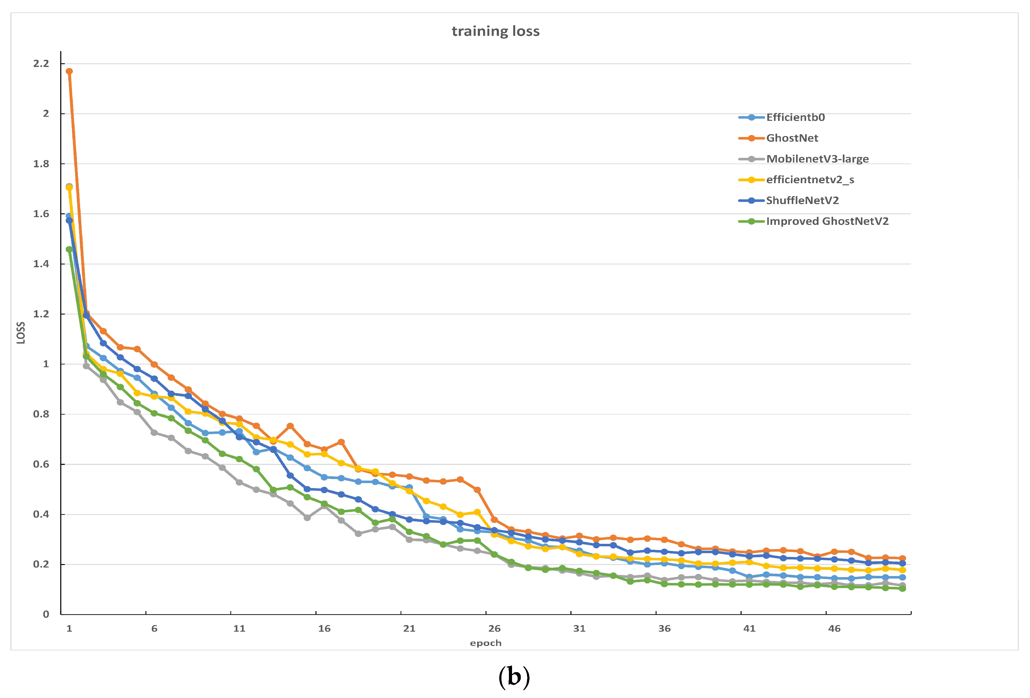
To test the effect of the improved GhostNetV2, we compared it with five lightweight models: GhostNet, MobileNetV3-large [35], EfficientNet-b0 [36], ShuffleNetV2 [37] and EfficientNetv2-S. Figure 15 is the training curve of the model. The training loss of the six models has the same convergence speed as the training ACC curve, and the training curve of the Ghost model fluctuates greatly. The improved GhostNetV2 model performs best in both training loss and training accuracy.
Table 4 shows the details of various model training, among which the accuracy of GhostNet is 92.56%, the number of parameters is 3.69 M, FLOPs is 0.15 G, and the training time is 1467 s. GhostNet has fewer parameters and FLOPs than other lightweight convolutional neural networks, but the accuracy is also lower. This table also lists the performance data of several other lightweight convolutional neural networks. ShuffleNetV2 has very few parameters and calculations, and the training time is at least 992 s, but the accuracy is low. The accuracy rates of MobileNetV3-large, EfficientNet-b0, and EfficientNetV2-S are similar. The training time of MobileNetV3-large is the shortest at 1263 s, and the amount of calculation is 0.23 G. The number of parameters and the amount of calculation of EfficientNetV2-S are larger, and the amount of calculation is equivalent to 7 times that of EfficientNet-b0, and the training time is 2.3 times that of EfficientNet-b0. Compared with other models, the effect shown by EfficientNet-b0 can only be regarded as quite satisfactory. The improved GhostNetV2 shows the best accuracy of 95.44%, the model training time is 1197 s, slightly higher than MobileNetV3-large, and the model parameters are 5.00 M, slightly lower than EfficientNet-b0. However, in terms of calculation, except for EfficientNetV2-S, the improved GhostNetV2 has the highest number of parameters.
4. Discussion
We discussed, in Section 3.1, the effect of four commonly used attention mechanisms on the model. SE calculates the attention weight of each channel through two layers of fully connected layers and global average pooling and then scales the features of each channel to enhance the feature channels that are important to the current task and weaken the feature channels that are irrelevant to the current task, but SE needs to use two fully connected layers to calculate channel attention weights, which will increase parameters and calculations. CA is a convolutional neural network utilizing multiple attention mechanisms, which consists of three modules: a combination of a spatial attention module, a channel attention module, and a scale attention module. It needs to introduce additional attention modules to calculate spatial, channel, and scale attention, which will lead to complex networks and more difficult calculations. CBAM is a module that integrates channel attention and spatial attention, which can dynamically adjust the importance of convolutional features. CBAM can consider the attention of both channel and space dimensions at the same time to better capture important features in the image, but CBAM needs to introduce additional modules to calculate channel and spatial attention, which will increase the complexity of the network and calculation volume. Efficient ECA can be embedded into existing CNN architectures to improve their performance. Its core idea is to use one-dimensional convolution to obtain local interaction information across channels and to control the coverage of the interaction by automatically adjusting the size of the convolution kernel. ECA avoids dimensionality reduction operations, thereby preserving complete information between channels. ECA uses fast 1D convolutions to achieve cross-channel interaction, which reduces the computational cost and parameter volume.
In Section 3.2, we explored the improvements in GhostNetV2. First of all, we considered that the Ghost module would lead to the insufficient learning ability of the model, so we optimized Ghost and added a channel shuffling operation in the Ghost module to enhance the information flow between feature maps. In view of the long training time of the model, we concluded from EfficientNetV2 that the depthwise convolution of the shallow layer of the network would lead to low model training efficiency, and the use of ordinary convolution in the shallow network could significantly improve the training speed, so we replaced the first five layers of the GhostNetV2 network for Fused-MBConv, the training time of the model was significantly reduced and the training efficiency was enhanced. Finally, we utilized ECA to further improve the performance of the model and reduce the parameters of the model. Although the calculation of the improved model became larger, its accuracy was higher and the training time was shorter, which was worth it.
We further tested the model with three public datasets (Rice Leaf Diseases Dataset, Plant-Village, and LWDCD2020) to evaluate its practical effect and generalization ability. The Rice Leaf Diseases Dataset contains images of rice leaves from different regions, with four different categories: healthy leaves, bacterial blight, brown spot, and sheath blight. Each category contains 300 RGB images with a resolution of 512 × 384 pixels, for a total of 1200 images. The Plant-Village dataset contains 54,303 pictures of plant leaves, which can be used to identify 38 plant disease datasets. LWDCD2020 contains about 4500 images covering four classes of wheat diseases. Table 5 shows the test performance of the improved model and four lightweight models on three public datasets. The test accuracy of the improved model on the Plant-Village, LWDCD2020, and Rice Leaf Diseases datasets reached 98.12%, 97.87%, and 99.12%, respectively. This shows that the improved GhostNetV2 has strong performance and generalization ability, and has excellent performance in crop disease recognition.
5. Conclusions
This study presented a method for identifying wheat yellow rust using optimized GhostNetV2, which can accurately and efficiently diagnose the severity of wheat yellow rust. Firstly, the Ghost module was improved, and the information transfer between feature maps was improved through the channel transformation operation so as to promote the feature learning ability of the model. Then, the Fused-MBConv module was used instead of the shallow network to shorten the training time of the model and increase the training efficiency. Finally, the ECA was used to further enhance the model’s attention to the disease and reduce the parameters of the model. We obtained accuracy rates of 98.22%, 98.82%, and 98.36% with the improved method on the Plant-Village, LWDCD2020, and Rice Leaf Diseases Dataset datasets, respectively, illustrating the generalization ability of the model. By improving the GhostNetV2 model, we achieved a 2.24% improvement in accuracy, a 37.49% reduction in training time, and a 1.16 M reduction in parameters. It is an effective technical means that can run quickly on mobile terminals. In the actual detection of disease severity, mobile devices can be used to detect diseases, and pesticides can be sprayed according to the guidance to reduce pollution and increase wheat yield.
However, the improved method also has shortcomings. The calculation load of the improved model increased by 0.48 G and had a higher calculation load. Future tasks will focus on how to further reduce the calculation load. Ultimately, we simply implemented severity detection for a single disease, but crop diseases are complex and diverse. Therefore, future work will further collect disease data to achieve severity identification of multiple diseases.
Author Contributions
Conceptualization, Z.L., X.F., T.Z. and Y.Z.; methodology, X.F.; software, Y.Z.; validation, Z.L. and Y.Z.; formal analysis, X.F. and Y.Z.; investigation, Z.L.; resources, X.F.; data curation, T.Z.; writing—original draft preparation, X.F.; writing—review and editing, Z.L.; visualization, Z.L. and T.Z.; supervision, Y.Z.; project administration, T.Z.; funding acquisition, T.Z. All authors have read and agreed to the published version of the manuscript.
Funding
This research received no external funding.
Institutional Review Board Statement
Not applicable.
Informed Consent Statement
Not applicable.
Data Availability Statement
The dataset is available at https://www.kaggle.com/datasets/tolgahayit/yellowrust19-yellow-rust-disease-in-wheat, accessed on 29 December 2022.
Acknowledgments
This work was supported by the National Key Research and Development Program of China: Research and Development of Quality Information Management and Control Technology for Efficient Connection of Grain Multimodal Transport (project no.: 2022YFD2100202).
Conflicts of Interest
The authors declare no conflict of interest.
References
- Wellings, C.R. Global status of stripe rust: A review of historical and current threats. Euphytica 2011, 179, 129–141. [Google Scholar] [CrossRef]
- Sabença, C.; Ribeiro, M.; Sousa, T.d.; Poeta, P.; Bagulho, A.S.; Igrejas, G. Wheat/Gluten-Related Disorders and Gluten-Free Diet Misconceptions: A Review. Foods 2021, 10, 1765. [Google Scholar] [CrossRef] [PubMed]
- Chai, Y.; Senay, S.; Horvath, D.; Pardey, P. Multi-peril pathogen risks to global wheat production: A probabilistic loss and investment assessment. Front. Plant Sci. 2022, 13, 1034600. [Google Scholar] [CrossRef] [PubMed]
- Biel, W.; Jaroszewska, A.; Stankowski, S.; Sobolewska, M.; Kępińska-Pacelik, J. Comparison of yield, chemical composition and farinograph properties of common and ancient wheat grains. Eur. Food Res. Technol. 2021, 247, 1525–1538. [Google Scholar] [CrossRef]
- YAO, F.-m.; LI, Q.-y.; ZENG, R.-y.; SHI, S.-q. Effects of different agricultural treatments on narrowing winter wheat yield gap and nitrogen use efficiency in China. J. Integr. Agric. 2021, 20, 383–394. [Google Scholar] [CrossRef]
- Nigam, S.; Jain, R.; Prakash, S.; Marwaha, S.; Arora, A.; Singh, V.K.; Singh, A.K.; Prakasha, T. Wheat Disease Severity Estimation: A Deep Learning Approach. In Proceedings of the Internet of Things and Connected Technologies: Conference Proceedings on 6th International Conference on Internet of Things and Connected Technologies (ICIoTCT), Patna, India, 29–30 July 2021; pp. 185–193. [Google Scholar]
- Jarošová, J.; Ripl, J.; Fousek, J.; Kundu, J.K. TaqMan Multiplex Real-Time qPCR assays for the detection and quantification of Barley yellow dwarf virus, Wheat dwarf virus and Wheat streak mosaic virus and the study of their interactions. Crop Pasture Sci. 2018, 69, 755–764. [Google Scholar] [CrossRef]
- Yuan, L.; Zhang, J.-C.; Wang, K.; Loraamm, R.-W.; Huang, W.-J.; Wang, J.-H.; Zhao, J.-L. Analysis of spectral difference between the foreside and backside of leaves in yellow rust disease detection for winter wheat. Precis. Agric. 2013, 14, 495–511. [Google Scholar] [CrossRef]
- Zhang, J.; Pu, R.; Loraamm, R.W.; Yang, G.; Wang, J. Comparison between wavelet spectral features and conventional spectral features in detecting yellow rust for winter wheat. Comput. Electron. Agric. 2014, 100, 79–87. [Google Scholar] [CrossRef]
- Ashourloo, D.; Aghighi, H.; Matkan, A.A.; Mobasheri, M.R.; Rad, A.M. An investigation into machine learning regression techniques for the leaf rust disease detection using hyperspectral measurement. IEEE J. Sel. Top. Appl. Earth Obs. Remote Sens. 2016, 9, 4344–4351. [Google Scholar] [CrossRef]
- Shi, Y.; Huang, W.; Luo, J.; Huang, L.; Zhou, X. Detection and discrimination of pests and diseases in winter wheat based on spectral indices and kernel discriminant analysis. Comput. Electron. Agric. 2017, 141, 171–180. [Google Scholar] [CrossRef]
- Khan, I.H.; Liu, H.; Li, W.; Cao, A.; Wang, X.; Liu, H.; Cheng, T.; Tian, Y.; Zhu, Y.; Cao, W. Early detection of powdery mildew disease and accurate quantification of its severity using hyperspectral images in wheat. Remote Sens. 2021, 13, 3612. [Google Scholar] [CrossRef]
- Mustafa, G.; Zheng, H.; Khan, I.H.; Tian, L.; Jia, H.; Li, G.; Cheng, T.; Tian, Y.; Cao, W.; Zhu, Y. Hyperspectral reflectance proxies to diagnose in-field fusarium head blight in wheat with machine learning. Remote Sens. 2022, 14, 2784. [Google Scholar] [CrossRef]
- Guan, Q.; Song, K.; Feng, S.; Yu, F.; Xu, T. Detection of Peanut Leaf Spot Disease Based on Leaf-, Plant-, and Field-Scale Hyperspectral Reflectance. Remote Sens. 2022, 14, 4988. [Google Scholar] [CrossRef]
- Mustafa, G.; Zheng, H.; Li, W.; Yin, Y.; Wang, Y.; Zhou, M.; Liu, P.; Bilal, M.; Jia, H.; Li, G. Fusarium head blight monitoring in wheat ears using machine learning and multimodal data from asymptomatic to symptomatic periods. Front. Plant Sci. 2022, 13, 1102341. [Google Scholar] [CrossRef]
- Liu, L.; Dong, Y.; Huang, W.; Du, X.; Ren, B.; Huang, L.; Zheng, Q.; Ma, H. A disease index for efficiently detecting wheat fusarium head blight using sentinel-2 multispectral imagery. IEEE Access 2020, 8, 52181–52191. [Google Scholar] [CrossRef]
- Schirrmann, M.; Landwehr, N.; Giebel, A.; Garz, A.; Dammer, K.-H. Early detection of stripe rust in winter wheat using deep residual neural networks. Front. Plant Sci. 2021, 12, 469689. [Google Scholar] [CrossRef]
- Hayit, T.; Erbay, H.; Varçın, F.; Hayit, F.; Akci, N. Determination of the severity level of yellow rust disease in wheat by using convolutional neural networks. J. Plant Pathol. 2021, 103, 923–934. [Google Scholar] [CrossRef]
- Deng, J.; Lv, X.; Yang, L.; Zhao, B.; Zhou, C.; Yang, Z.; Jiang, J.; Ning, N.; Zhang, J.; Shi, J. Assessing Macro Disease Index of Wheat Stripe Rust Based on Segformer with Complex Background in the Field. Sensors 2022, 22, 5676. [Google Scholar] [CrossRef]
- Gao, Y.; Wang, H.; Li, M.; Su, W.-H. Automatic Tandem Dual BlendMask Networks for Severity Assessment of Wheat Fusarium Head Blight. Agriculture 2022, 12, 1493. [Google Scholar] [CrossRef]
- Mao, R.; Wang, Z.; Li, F.; Zhou, J.; Chen, Y.; Hu, X. GSEYOLOX-s: An Improved Lightweight Network for Identifying the Severity of Wheat Fusarium Head Blight. Agronomy 2023, 13, 242. [Google Scholar] [CrossRef]
- Hayıt, T.; Erbay, H.; Varçın, F.; Hayıt, F.; Akci, N. The classification of wheat yellow rust disease based on a combination of textural and deep features. Multimed. Tools Appl. 2023, 1–19. [Google Scholar] [CrossRef]
- Liu, X.; Xie, Q.; Zhao, Q.; Wang, H.; Meng, D. Low-light image enhancement by Retinex based algorithm unrolling and adjustment. arXiv 2022, arXiv:2202.05972. [Google Scholar] [CrossRef] [PubMed]
- Howard, A.G.; Zhu, M.; Chen, B.; Kalenichenko, D.; Wang, W.; Weyand, T.; Andreetto, M.; Adam, H. Mobilenets: Efficient convolutional neural networks for mobile vision applications. arXiv 2017, arXiv:1704.04861. [Google Scholar]
- Zhang, X.; Zhou, X.; Lin, M.; Sun, J. Shufflenet: An extremely efficient convolutional neural network for mobile devices. In Proceedings of the IEEE Conference on Computer Vision and Pattern Recognition, Salt Lake City, UT, USA, 18–23 June 2018; pp. 6848–6856. [Google Scholar]
- Han, K.; Wang, Y.; Tian, Q.; Guo, J.; Xu, C.; Xu, C. Ghostnet: More features from cheap operations. In Proceedings of the IEEE/CVF Conference on Computer Vision and Pattern Recognition, Seattle, WA, USA, 13–19 June 2020; pp. 1580–1589. [Google Scholar]
- Tang, Y.; Han, K.; Guo, J.; Xu, C.; Xu, C.; Wang, Y. GhostNetV2: Enhance Cheap Operation with Long-Range Attention. arXiv 2022, arXiv:2211.12905. [Google Scholar]
- Tan, M.; Le, Q. Efficientnetv2: Smaller models and faster training. In Proceedings of the International Conference on Machine Learning, Virtual, 18–24 July 2021; pp. 10096–10106. [Google Scholar]
- Hu, J.; Shen, L.; Sun, G. Squeeze-and-excitation networks. In Proceedings of the IEEE Conference on Computer Vision and Pattern Recognition, Salt Lake City, UT, USA, 18–23 June 2018; pp. 7132–7141. [Google Scholar]
- Wang, Q.; Wu, B.; Zhu, P.; Li, P.; Zuo, W.; Hu, Q. ECA-Net: Efficient channel attention for deep convolutional neural networks. In Proceedings of the IEEE/CVF Conference on Computer Vision and Pattern Recognition, Seattle, WA, USA, 13–19 June 2020; pp. 11534–11542. [Google Scholar]
- Fang, X.; Zhen, T.; Li, Z. Lightweight Multiscale CNN Model for Wheat Disease Detection. Appl. Sci. 2023, 13, 5801. [Google Scholar] [CrossRef]
- Gu, R.; Wang, G.; Song, T.; Huang, R.; Aertsen, M.; Deprest, J.; Ourselin, S.; Vercauteren, T.; Zhang, S. CA-Net: Comprehensive attention convolutional neural networks for explainable medical image segmentation. IEEE Trans. Med. Imaging 2020, 40, 699–711. [Google Scholar] [CrossRef]
- Woo, S.; Park, J.; Lee, J.-Y.; Kweon, I.S. Cbam: Convolutional block attention module. In Proceedings of the European Conference on Computer Vision (ECCV), Munich, Germany, 8–14 September 2018; pp. 3–19. [Google Scholar]
- Selvaraju, R.R.; Cogswell, M.; Das, A.; Vedantam, R.; Parikh, D.; Batra, D. Grad-cam: Visual explanations from deep networks via gradient-based localization. In Proceedings of the IEEE International Conference on Computer Vision, Venice, Italy, 22–29 October 2017; pp. 618–626. [Google Scholar]
- Howard, A.; Sandler, M.; Chu, G.; Chen, L.-C.; Chen, B.; Tan, M.; Wang, W.; Zhu, Y.; Pang, R.; Vasudevan, V. Searching for mobilenetv3. In Proceedings of the IEEE/CVF International Conference on Computer Vision, Seoul, Republic of Korea, 27 October–2 November 2019; pp. 1314–1324. [Google Scholar]
- Tan, M.; Le, Q. Efficientnet: Rethinking model scaling for convolutional neural networks. In Proceedings of the International Conference on Machine Learning, Long Beach, CA, USA, 10–15 June 2019; pp. 6105–6114. [Google Scholar]
- Ma, N.; Zhang, X.; Zheng, H.-T.; Sun, J. Shufflenet v2: Practical guidelines for efficient cnn architecture design. In Proceedings of the European Conference on Computer Vision (ECCV), Munich, Germany, 8–14 September 2018; pp. 116–131. [Google Scholar]
- Hughes, D.; Salathé, M. An open access repository of images on plant health to enable the development of mobile disease diagnostics. arXiv 2015, arXiv:1511.08060. [Google Scholar]
- Goyal, L.; Sharma, C.M.; Singh, A.; Singh, P.K. Leaf and spike wheat disease detection & classification using an improved deep convolutional architecture. Inform. Med. Unlocked 2021, 25, 100642. [Google Scholar]
- Sethy, P.K.; Barpanda, N.K.; Rath, A.K.; Behera, S.K. Deep feature based rice leaf disease identification using support vector machine. Comput. Electron. Agric. 2020, 175, 105527. [Google Scholar] [CrossRef]
Figure 1.
The severity of wheat yellow rust.

Figure 2.
Image enhancement. (a) Original image; (b) enhanced image.

Figure 3.
Feature Map.

Figure 4.
Vanilla Convolution.

Figure 5.
The Ghost module.

Figure 6.
The information flow of DFC attention.

Figure 7.
The GhostNet bottleneck map. (a) GhostNet bottleneck; (b) GhostNetV2 bottleneck and DFC.

Figure 8.
The CS-Ghost Module.

Figure 9.
Structure of MBConv and Fused-MBConv.

Figure 10.
ECA structure diagram.

Figure 11.
Accuracy in training.

Figure 12.
Heat map of four experiments.

Figure 13.
Feature map. (a) Improved model Block1 features; (b) improved model Block2 features; (c) original model block features.
Figure 13.
Feature map. (a) Improved model Block1 features; (b) improved model Block2 features; (c) original model block features.

Figure 14.
Confusion Matrix.

Figure 15.
Six model training results. (a) Accuracy curve; (b) loss curve.


Table 1.
Model Architectures.
| Stage | Input | Operator | Stride | ECA | #exp | Output |
|---|---|---|---|---|---|---|
| Stem | 224 × 224 | Conv2d 3×3 | 2 | - | 16 | 112 × 112 |
| Block1 | 112 × 112 | FusedMBConv | 1 | - | 16 | 112 × 112 |
| 112 × 112 | FusedMBConv | 2 | - | 40 | 56 × 56 | |
| 56 × 56 | FusedMBConv | 1 | - | 40 | 56 × 56 | |
| 56 × 56 | FusedMBConv | 2 | - | 80 | 28 × 28 | |
| 28 × 28 | FusedMBConv | 1 | - | 80 | 28 × 28 | |
| Block2 | 28 × 28 | CS-bneck | 2 | - | 240 | 14 × 14 |
| 14 × 14 | CS-bneck | 1 | - | 200 | 14 × 14 | |
| 14 × 14 | CS-bneck | 1 | - | 184 | 14 × 14 | |
| 14 × 14 | CS-bneck | 1 | - | 184 | 14 × 14 | |
| 14 × 14 | CS-bneck | 1 | 1 | 480 | 14 × 14 | |
| 14 × 14 | CS-bneck | 1 | 1 | 672 | 14 × 14 | |
| 14 × 14 | CS-bneck | 2 | 1 | 672 | 7 × 7 | |
| 7 × 7 | CS-bneck | 1 | - | 960 | 7 × 7 | |
| 7 × 7 | CS-bneck | 1 | 1 | 960 | 7 × 7 | |
| 7 × 7 | CS-bneck | 1 | - | 960 | 7 × 7 | |
| 7 × 7 | CS-bneck | 1 | 1 | 960 | 7 × 7 | |
| Head | 7 × 7 | AvgPool | - | - | - | 1 × 1 |
| 1 × 1 | Conv2d 1×1 | 1 | - | - | 1 × 1 | |
| 1 × 1 | Fc | - | - | - | 1 × 1000 |
#exp means expansion size.
Table 2.
Effect of attentional mechanisms on the model.
| Attention | Accuracy (%) | Precision(%) | Recall (%) | F1 Score (%) | Time (s) | Param (M) |
|---|---|---|---|---|---|---|
| ES | 93.20 | 92.96 | 92.97 | 92.96 | 2847 | 6.16 |
| CA | 94.16 | 94.09 | 94.06 | 94.07 | 1888 | 5.22 |
| CBAM | 94.24 | 94.07 | 94.00 | 94.04 | 1970 | 5.03 |
| ECA | 94.96 | 94.98 | 94.83 | 94.91 | 1850 | 4.65 |
Table 3.
Improvement in the method on the model results.
| Method | CS-Ghost | Fused-MBConv | ECA | Accuracy (%) | F1 Score (%) | Time (s) | Param (M) | FlOPs (G) | Infer-Time (ms) |
|---|---|---|---|---|---|---|---|---|---|
| GhostNetV2 | × | × | × | 93.20 | 92.96 | 1915 | 6.16 | 0.18 | 28.52 |
| GhostNetV2_A | √ | × | × | 94.68 | 94.56 | 1978 | 6.18 | 0.18 | 33.07 |
| GhostNetV2_B | √ | √ | × | 94.76 | 94.62 | 1242 | 6.20 | 0.66 | 31.12 |
| GhostNetV2_C | √ | √ | √ | 95.44 | 95.30 | 1197 | 5.00 | 0.66 | 27.94 |
Table 4.
Training results of seven models.
| Model | Accuracy (%) | Precision (%) | Recall (%) | F1 Score (%) | Training-Time (s) | Param (M) | FlOPs (G) |
|---|---|---|---|---|---|---|---|
| GhostNet | 92.56 | 92.42 | 92.50 | 92.46 | 1467 | 3.69 | 0.15 |
| MobileNetV3-large | 94.96 | 94.92 | 94.81 | 94.87 | 1263 | 5.56 | 0.23 |
| EfficientNet-b0 | 94.40 | 94.19 | 94.27 | 94.23 | 1851 | 5.38 | 0.40 |
| ShuffleNetV2 | 93.44 | 93.25 | 93.28 | 93.26 | 992 | 3.50 | 0.30 |
| EfficientNetv2-S | 94.08 | 94.09 | 93.87 | 93.98 | 4264 | 21.46 | 2.87 |
| Improved GhostNetV2 | 95.44 | 95.33 | 95.27 | 95.30 | 1197 | 5.00 | 0.66 |
Table 5.
Test results for the three datasets with the improved model.
| Data | Model | Accuracy (%) | Precision (%) | Recall (%) | F1 Score (%) |
|---|---|---|---|---|---|
| Plant-Village [38] | Improved GhostNetV2 | 98.12 | 98.05 | 98.09 | 98.07 |
| MobileNetV3-Large | 98.57 | 98.70 | 98.63 | 98.67 | |
| EfficientNet-b0 | 98.76 | 99.71 | 98.71 | 98.71 | |
| ShuffleNetV2 | 98.52 | 98.49 | 98.43 | 98.46 | |
| MobileNetV2 | 97.83 | 97.43 | 97.94 | 97.72 | |
| LWDCD2020 [39] | Improved GhostNetV2 | 97.87 | 97.93 | 97.91 | 97.92 |
| MobileNetV3-Large | 96.58 | 96.66 | 96.67 | 96.67 | |
| EfficientNet-b0 | 97.17 | 97.26 | 9720 | 97.23 | |
| ShufflenetV2 | 93.22 | 93.53 | 93.19 | 93.36 | |
| MobileNetV2 | 92.81 | 92.96 | 92.82 | 92.89 | |
| Rice Leaf Diseases Dataset [40] | Improved GhostNetV2 | 99.12 | 99.21 | 99.16 | 99.19 |
| MobileNetV3-Large | 99.66 | 99.64 | 99.64 | 99.64 | |
| EfficientNet-b0 | 99.32 | 99.38 | 99.30 | 99.34 | |
| ShuffleNetV2 | 98.73 | 98.79 | 98.76 | 98.77 | |
| MobileNetV2 | 96.28 | 96.37 | 96.37 | 96.37 |
Disclaimer/Publisher’s Note: The statements, opinions and data contained in all publications are solely those of the individual author(s) and contributor(s) and not of MDPI and/or the editor(s). MDPI and/or the editor(s) disclaim responsibility for any injury to people or property resulting from any ideas, methods, instructions or products referred to in the content. |
© 2023 by the authors. Licensee MDPI, Basel, Switzerland. This article is an open access article distributed under the terms and conditions of the Creative Commons Attribution (CC BY) license (https://creativecommons.org/licenses/by/4.0/).
Share and Cite
MDPI and ACS Style
Li, Z.; Fang, X.; Zhen, T.; Zhu, Y. Detection of Wheat Yellow Rust Disease Severity Based on Improved GhostNetV2. Appl. Sci. 2023, 13, 9987. https://0-doi-org.brum.beds.ac.uk/10.3390/app13179987
AMA Style
Li Z, Fang X, Zhen T, Zhu Y. Detection of Wheat Yellow Rust Disease Severity Based on Improved GhostNetV2. Applied Sciences. 2023; 13(17):9987. https://0-doi-org.brum.beds.ac.uk/10.3390/app13179987
Chicago/Turabian StyleLi, Zhihui, Xin Fang, Tong Zhen, and Yuhua Zhu. 2023. "Detection of Wheat Yellow Rust Disease Severity Based on Improved GhostNetV2" Applied Sciences 13, no. 17: 9987. https://0-doi-org.brum.beds.ac.uk/10.3390/app13179987
Note that from the first issue of 2016, this journal uses article numbers instead of page numbers. See further details here.