
Modelling the Structure and Anisotropy of London Clay Using the SA_BRICK Model
1
Faculty of Civil and Geodetic Engineering, University of Ljubljana, 1000 Ljubljana, Slovenia
2
IRGO, Institute for Mining, Geotechnology and Environment, 1000 Ljubljana, Slovenia
*
Author to whom correspondence should be addressed.
Appl. Sci. 2023, 13(2), 880; https://0-doi-org.brum.beds.ac.uk/10.3390/app13020880
Submission received: 11 December 2022
/
Revised: 31 December 2022
/
Accepted: 3 January 2023
/
Published: 9 January 2023
(This article belongs to the Special Issue Recent Progress on Advanced Foundation Engineering)
Abstract
:Several constitutive models had been developed by other researchers to cover the main features of mechanical behaviour of natural overconsolidated clays, such as the nonlinear stress–strain response at small and large strains, and the recent stress history effect. Kinematic hardening models include these features to facilitate realistic predictions of soil–structure interaction. This paper presents the further development of a kinematic hardening model BRICK that includes anisotropy and the influence of soil structure on the mechanical behaviour of a natural clay. High quality laboratory tests were used to calibrate the input parameters of the model in a single element configuration, and a documented boundary value problem of tunnel excavation was used to validate the model in finite element calculations. A comprehensive comparative study between the predictions of different kinematic hardening models, using two different software packages, was carried out. It was observed that the SA_BRICK model is in fair agreement with the observed data and gives improved predictions in comparison to other kinematic hardening models, particularly in terms of narrowness of the settlement trough above the tunnel. Advanced predictions of ground deformations caused by tunnel excavations can be effectively used to mitigate possible damage of existing structures affected by tunnelling in an urban environment.
1. Introduction
Advances in the laboratory testing have contributed to a better understanding of the non-linear behaviour of natural stiff clays at small and large strains. Constitutive models, which are widely applied to simulate soil–structure interaction using numerical analyses, have been developed in parallel with advances in laboratory testing. This development started some fifty years ago with simple nonlinear elastic models [1,2] and early works on elastic–plastic models using kinematic hardening [3] and bounding surface concepts [4]. These were further improved by more advanced kinematic hardening models, which can describe both the nonlinearity and plastic behaviour in the initial stages of loading using a single kinematic surface (e.g., [5]). Further development included the capability of modelling the recent stress history effect [6] using two kinematic surfaces inside the state boundary surface (e.g., [7]). The BRICK model, initially developed by Simpson [8] for overconsolidated clays, has the ability to model the non-linear stress–strain response of soil and the recent stress history effect, both of which are the main manifestations of the mechanical behaviour characterised by kinematic hardening.
With the development of the fundamental understanding of the behaviour of structural soils [9,10] and similarities in the behaviour of hard soils and soft rocks [11], there were further advances in kinematic hardening models to include other aspects of natural materials behaviour, such as structure and anisotropy [12,13,14]. The BRICK model was further developed to include the structural behaviour of hard soils and soft rocks [15,16] and was successfully validated on three natural materials: Pappadai clay, North Sea clay and Corinth Marl, thus covering a wide range of natural structured materials. Ellison et al. [17] introduced anisotropy into the BRICK model, which resulted in an evident improvement in the prediction of the behaviour of London clay.
This paper presents further development of the BRICK model to include both anisotropy and structure in modelling the behaviour of a natural stiff clay, namely the SA_BRICK model. The SA_BRICK model was firstly validated using single element predictions of computed stress paths and stiffnesses with laboratory test results for undrained shearing in compression and extension. The high-quality laboratory triaxial test results on London clay [18] were used and compared with the numerical predictions of the SA_BRICK model. After the validation in single element form, the model was developed for a generalised three-dimensional (3D) stress state and integrated in the finite element program PLAXIS [19]. The predictions of a full-sized boundary value problem were carried out in the study of the excavation of the Jubilee Line tunnels at St. James’s Park in London, UK [20]. A considerable improvement in the prediction of the settlement trough above the tunnel was calculated, proving that the BRICK model can be successfully upgraded to include anisotropy and structure in modelling the behaviour of London clay.
Recent Developments in the Modelling of the Behaviour of London Clay
The development of sophisticated measuring devices in the laboratory and in situ resulted in a better understanding of the clay composition and structure (e.g., [21,22,23,24]) and clay shear strength behaviour [25]. A comprehensive overview of the geological history and geotechnical and geomechanical characteristics of London clay is given by Hight et al. [26]. Their work was based on the data obtained from ground investigations for Terminal 5 at London’s Heathrow Airport, which was also the lithological unit used in this research. London clay is a typical heavily overconsolidated marine clay of mineral composition comprising illite, chlorite, kaolinite, smectite and montmorillonite. At the Terminal 5 site, the clay was of high to very high plasticity, in which the plasticity index (PI) averaged around 40% (minimum of 33% and maximum of 49%), while the liquid limit (LL) was between 65 and 70%. The same lithological unit at St. James’s Park had similar index properties, with an average mass water content of 20% to 25% and a unit weight varying between 20 kN/m3 and 22 kN/m3 [27]. The coefficient of permeability of London clay typically varies between k = 1 × 10⁻⁹ m/s and k = 1 × 10⁻¹⁰ m/s. In terms of the strength effective stress parameters, the apparent cohesion is characteristically taken as c′ = 0, while the angle of shear resistance ranges from a peak of Φ′ = 25°, to a large strain of Φ′ = 20°, and to residual values of Φ′ = 12° [26].
Following progressive digitalisation of the test control and instrumentation in the laboratory, further research highlighted the importance of structure in governing the behaviour of London clay [18,28]. In this context, the role of anisotropy at small and large strain levels [29,30] and the influence of recent stress history, creep and rates of loading on stiffness at small strains [28,31] were extensively studied. A comprehensive overview of the role of structure in the behaviour of London clay at different observed scales was given by Yeow and Coop [32]. They highlighted that unfissured samples were found to be considerably stronger than equivalent reconstituted samples at similar void ratios and stress levels, while this effect was less pronounced in terms of stiffness, in particular at small strains. Using scanning electron micrographs (SEMs), Gasparre et al. [28] showed significant differences in the micro-fabric between natural and reconstituted samples, so that a denser and more orientated packing of natural samples was found at greater depths. An increase in the anisotropy of stiffness with depth was found to be dependent on the increased stress level and the change in the sub-unit. This was manifested as an increase in the ratio of anisotropy (defined in terms of the ratio of the horizontal to the vertical Young’s modulus; Eh/Ev), starting from slightly less than 2 at the top of strata to nearly 3 at 30 m depth. Additionally, the ratio of shear moduli remains nearly constant at around 1.5 at all depths, as previously observed by Simpson et al. [33].
In terms of the macro-fabric, the natural fissures are found within the London clay at all depths and present principal manifestation of a noticeable anisotropy of strength [30]. It was also shown that the presence of fissures can significantly lower the peak strength of a sample, when compared to samples which fail due to strain localisation. Gasparre et al. [18] found that structure has a pronounced effect on the compressibility and strength of London clay, and a significant effect on the anisotropy of stiffness and strength. These effects were observed to be relatively stable and do not break down rapidly with straining, particularly in compression [34].
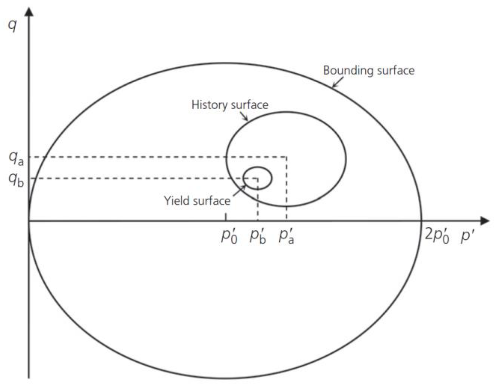
The 3SKH (three-surface kinematic hardening) model of Stallebrass and Taylor [7] (Figure 1) was also used to model natural London clay. Apart from the yield surface and bounding surface, the third history surface is defined as an envelope of points where the stiffness no longer depends on the previous loading history. Both the BRICK and 3SKH models were used effectively to model the behaviour of London clay, notwithstanding that neither of the two models expressly account for the effects of anisotropy and structure. The 3SKH model was improved by Grammatikopoulou et al. [35], further referred to as the M3-SKH model, for the generalised three-dimensional (3D) stress state. The improvement contained a different hardening modulus, to model a smooth elastic–plastic transition, compared to the original 3SKH formulation, in which a marked drop in stiffness occurred once plasticity was engaged. Yeow and Coop [32] compared laboratory triaxial data on London clay from Gasparre et al. [28] with the predictions of the original BRICK and M3-SKH models, highlighting the advantages and deficiencies of both models.
2. Development of the BRICK Model
2.1. Original BRICK Model Formulation
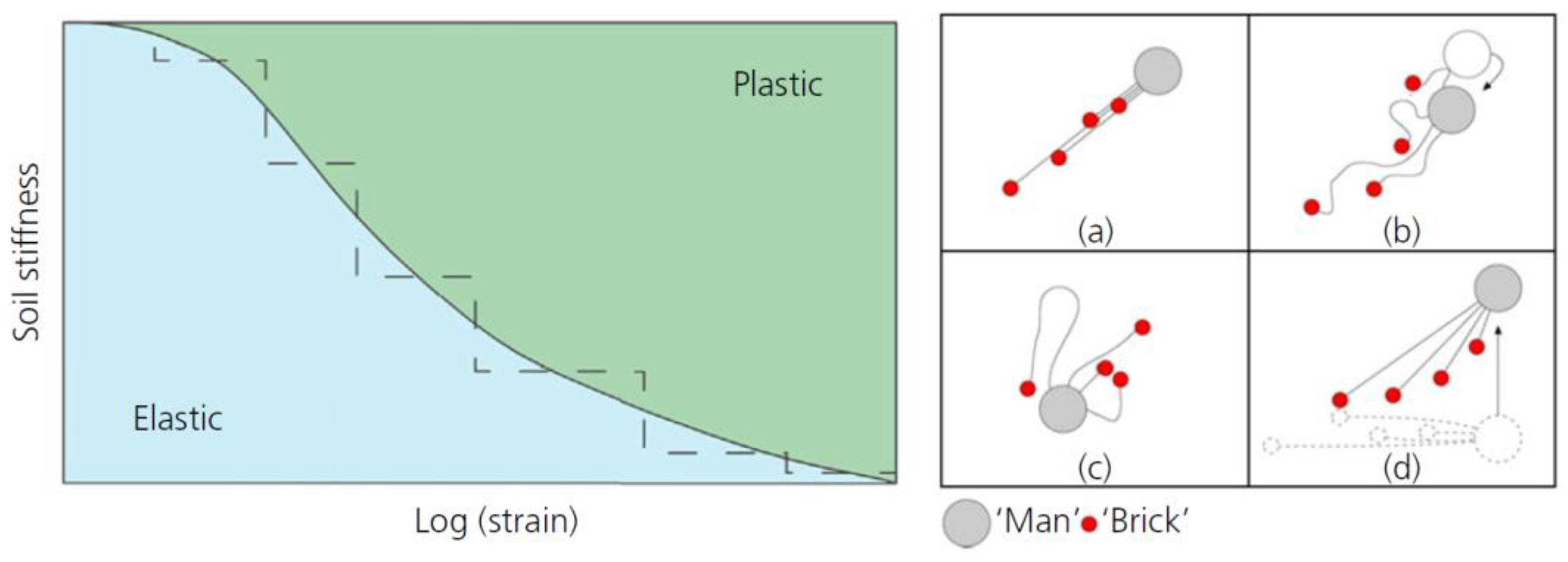
Different versions of the BRICK model have been developed, so far giving satisfactory numerical predictions for various geotechnical problems. The original BRICK model in plane strain was developed [8] specifically to model natural London clay, although not accounting for structure. The BRICK model was originally developed to model the recent stress history effect [6] using an analogy of a man dragging a series of bricks on strings behind him in a strain space at different lengths (Figure 2). As the man changes his direction of movement, the various strings become loose until the bricks re-engage, so that the strings fall into line behind the man again and become tight. The model is formulated so that the movement of each brick directly represents the development of plastic strain for a specified proportion of the material. This means that the model behaviour is fully elastic when all strings are loose. In contrast, the behaviour is fully plastic when all strings are tight, so that the bricks are lined up behind the man and are normal to the volumetric strain axis. It is assumed that only elastic strains cause stress changes. The effect of recent stress history is, therefore, modelled by the disposition of memory points defining the approach loading path [8], so that the stiffness decay curve is essentially a model parameter (as each brick corresponds to plastic strain for a specified proportion of the material, the string lengths define the shape of the stiffness decay curve). The important feature of the model is that if the tangent shear modulus Gtan is normalised by the mean stress, s′ = (σx′ +σy′)/2, and then plotted against the shear strain, γ, the area under the curve is equal to sin ϕ′.
The original BRICK parameters used to model the London clay are presented in Table 1. The string lengths are defined against normalised shear modulus (G/Gmax) to cover the full range of shear strains. The parameters λ* and κ* are the gradients of the compression and swelling lines in the plane. The parameter ι defines the ratio of elastic stiffness to mean effective stress p′, and ν is the Poisson’s ratio. The BRICK model adopts a linear relationship between the logarithm of the overconsolidation ratio (OCR) and stiffness, whereas the original parameter is divided into two components, and , to separate the influence of overconsolidation on the stiffness and strength, respectively.
The original formulation of the BRICK model was successfully used to evaluate the deformation and stability response of the platform in the North Sea [36], which was founded on heavily overconsolidated and structured clays. The effect of structure was accounted for by a careful calibration of the artificial degree of consolidation, which was needed to accurately model undrained shear strength of a structured stiff clay.
2.2. Continuous Developments of Constitutive Models Based on the BRICK Model Formulation
To realistically model glacial till, the original BRICK model was extended [37] by utilising the volumetric strain axis and five shear strain axes. Clarke and Hird [38] introduced the viscous behaviour in the BRICK model, including creep and strain rate dependent stiffness, by presenting two approaches, changing either the velocity of the bricks or the string length (i.e., the SRD BRICK model). Tuxworth [39] modified the BRICK model to improve the simulations of the recent stress history effects of clays. Cudny and Partyka [40] utilised the BRICK concept in their constitutive model for simulating the degradation of stiffness in the intermediate strain region, including the effects of strain history. The same author added a new small strain extension to the conventional elastic-plastic Hardening Soil model to overcome the overshooting problems by combining it with the BRICK model (i.e., so called HS-BRICK model) [41]. The developments of the BRICK model to account for the structure and anisotropy of natural stiff clays are shown in more detail in the next section.
3. Developments of the SA_BRICK Model
3.1. Modelling of the Structure
The state of overconsolidation affects the behaviour of the BRICK model by the modification of string lengths and elastic shear modulus (kPa) according to the following formulae (Equations (1) and (2)):
where is the initial string length of brick for the normally consolidated material, are are the variables that take into account the increase in stiffness and strength due to the overconsolidation, respectively, while (kPa) is the current isotropic elastic bulk modulus and is Poisson’s ratio on the normal consolidation line as a material parameter. The extent of overconsolidation is measured by the difference in the volumetric strain between a current state and the state on the normal compression line (NCL) in the form of a state parameter :
where and are the current volumetric strain and mean effective stress, respectively, while the subscript 0 refers to the initial reference state at the NCL. The state parameter affects the evaluation of variables and by the following formulae:
where and are material parameters. Additionally, the state in the plane influences the current value of the volumetric stiffness variable as
where is the volumetric stiffness material parameter.
Vukadin [15] and Vukadin and Jovičić [16] introduced the influence of structure in the original BRICK model and named the improved model S_BRICK. The structure was incorporated into the model by adding two variables, namely and . The variable was used to proportionally increase or decrease the original string lengths , having the effect of changing the area beneath the S-shaped curve . Parameter was introduced into Equation (1) as follows:
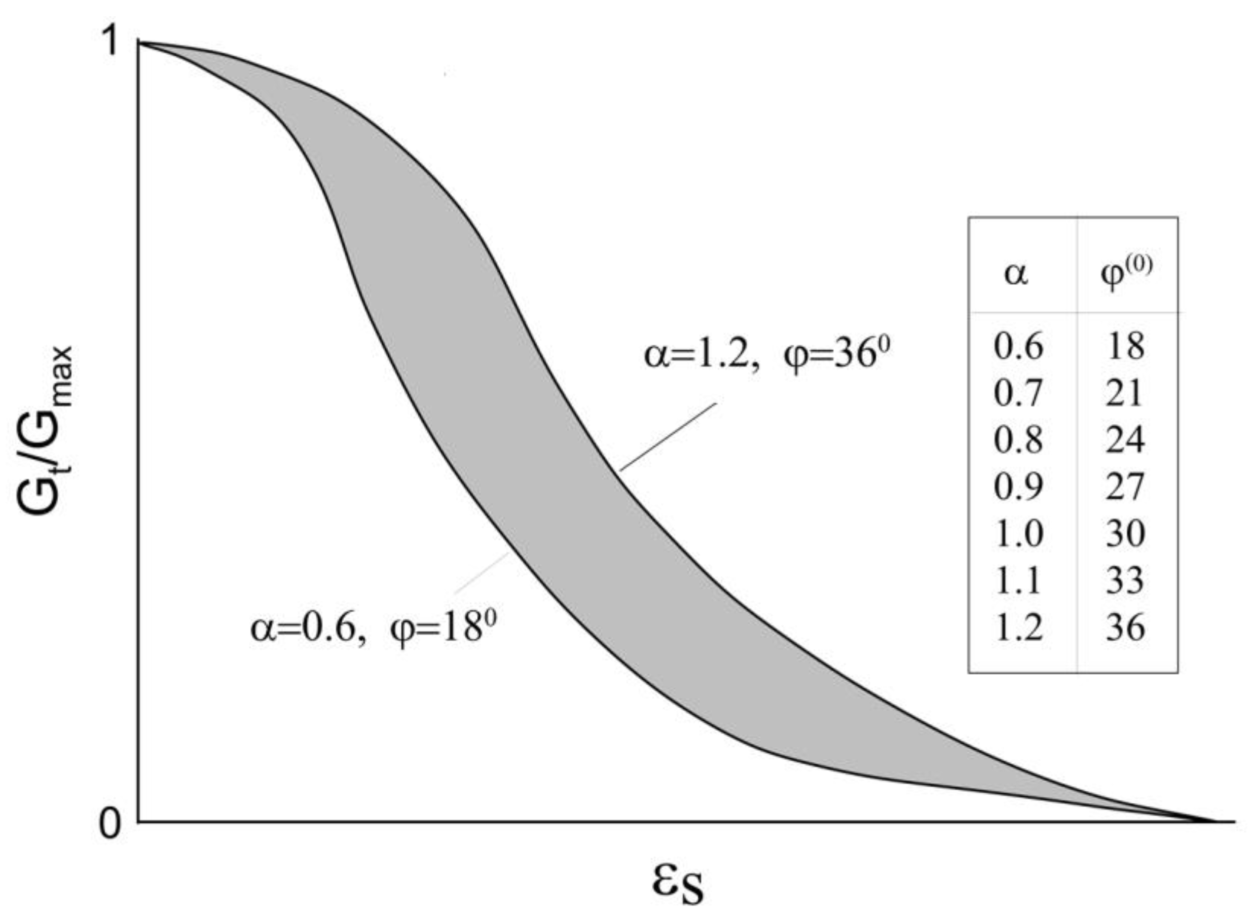
Given that the area under the S-shaped curve is proportional to sin ϕ′, this modification directly influences the value of the maximum angle of the shearing resistance, i.e., the strength response of the model. The applicable range of for natural materials was chosen so that the angle of shearing resistance lies within the range from to for the normally consolidated states (Figure 3).
The second introduced variable to consider the effect of the structure on stiffness in the BRICK model was . It is introduced to modify the state parameter (see Equation (3)) as follows:
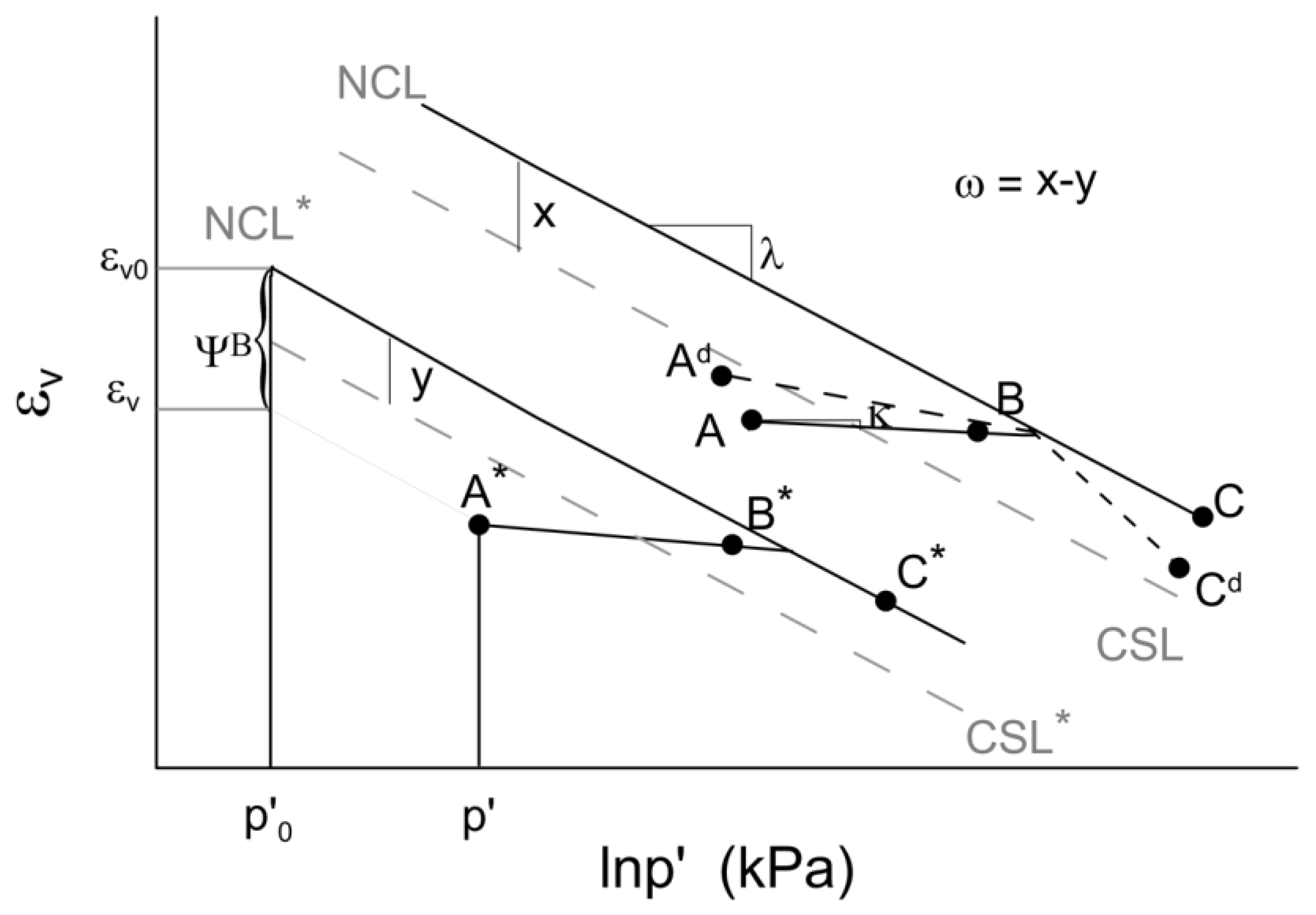
The concept of is graphically represented in Figure 4 in the plane, in which NCL and the critical state line (CSL) are shown for a structured and a reconstituted sample (marked with *). Its effect can easily be understood as an increase in the distance between the normal compression line and the critical state line in terms of volumetric strain as a consequence of structure, in comparison with that distance on the reconstituted material. This increase in distance and the apparent overconsolidation of the soil are directly superimposed.
Additionally, S_BRICK enables the modelling of destructuring. Further details of the formulation can be found in [16].
It can be seen from Equations (4)–(7) that the state parameter influences both the volumetric stiffness and the string lengths . Additionally, the string lengths are affected by the value of parameter (Equation (7)). Thus, there was an overlapping influence of both structure parameters and in the S_BRICK model. As a consequence, the model calibration procedure was less clear and required iterative procedures due to the dependence of on and vice versa.
In the formulation of the SA_BRICK model, the parameter was removed from the evaluation of the state (Equation (8)) and used in the evaluation of the volumetric stiffness variable as follows:
In this way, the influence of structure on the model behaviour is taken into account via the parameters and independently. The parameter modifies the current strength of the material via the string lengths (Equation (7)), while the parameter modifies the current stiffness (Equation (9)). A summary of the used formulations of the structure effects in the BRICK, S_BRICK and SA_BRICK models is given in Table 2.
3.2. Modelling of the Anisotropy
A comprehensive overview of the anisotropy of London clay and its modelling was given by Wongsaroj et al. [42]. As other soils are deposited over a large lateral extent, London clay is best described as cross-anisotropic; it responds differently when compressed in the vertical and horizontal directions but responds in the same way if compressed in either of the two horizontal directions. In terms of elastic behaviour, only five constants are required to define cross-anisotropy [43]. Ellison et al. [44] modified the basic BRICK model by adding the plastic strain reduction through the volumetric strain hardening by brick repositioning and formulating the model in the general strain space. Additionally, the stiffness anisotropy was introduced by transforming the coordinate system in which the model was based and adding an anisotropic stiffness matrix, as explained bellow. The same approach to account for the anisotropy was chosen here for upgrading the S_BRICK model to the SA_BRICK model. The important difference between the work of Ellison et al. [44] and this research was that the bricks were not repositioned in the SA_BRICK model but remained in the same original shape and form as in the original BRICK model (i.e., as defined by the shape of the S curve, that is, by the string lengths and corresponding normalised shear stiffnesses G/Gmax, as given in Table 1).
The introduction of anisotropy was carried out following Ellison et al. [17], by using the transformation matrix defined by Equation (10):
where is the isotropic compliance matrix and the anisotropic stiffness matrix. and take the following form in Cartesian coordinates by using the bulk modulus and Poisson’s ratio at state on the normal consolidation line :
where the meaning of the above terms is as follows:
As can be seen from Equations (12)–(16), only three additional parameters are needed to fully define anisotropy , namely Young’s modulus ratio , the shear modulus ratio and Poisson’s ratio in the horizontal plane . By utilising the matrix , the strain increments are transformed into the modified strain increments by the following expressions [17]:
The BRICK model operates in the BRICK coordinate system with the stress and strain components and , and transformations between Cartesian and BRICK coordinate systems are needed by utilising the transformation matrices and as follows:
The BRICK formulation takes into account that when a soil material undergoes shearing, the bricks start to slide past one another until the condition of constant volume (i.e., critical state) is reached. Therefore, the modelling of coupling between shear and volumetric components must evolve to reach the state of no coupling. To achieve this, the evolutional variable was introduced into the matrix from Equation (11), which is designated as :
in which represents the degree of string mobilisation in the direction of strain increment:
where is the additional parameter and is a measure of the alignment of strings in the direction of strain increment :
The number is the number of bricks in each stress point, is the proportion of material represented by brick , is the string length of brick , is the mobilised string length of brick in the direction of the strain increment and is a parameter which considers the Lode angle effects on string lengths. More details of this transformation are given in [45].
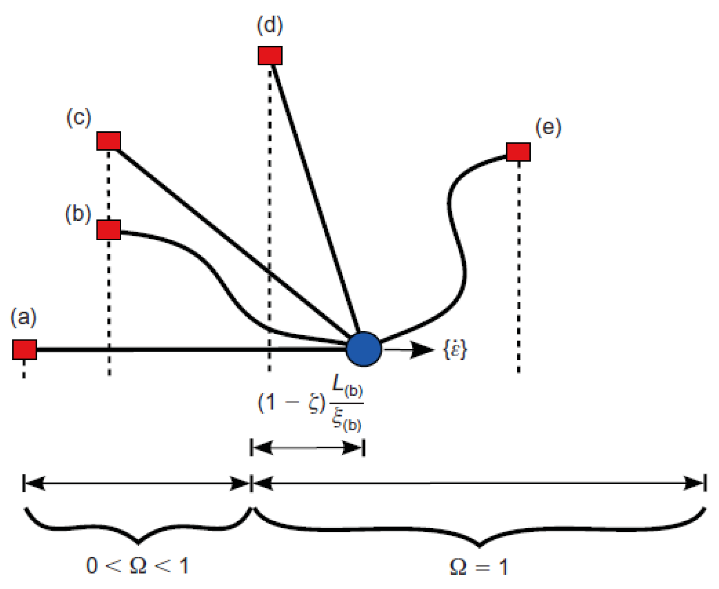
By using the parameter , the threshold string alignment is defined with the value . If is reduced below , then parameter , meaning that strings are becoming less aligned in the direction of strain increment. In this case, full anisotropy is taking place. On the other hand, by increasing over , the parameter starts to reduce according to the transformation from 1 towards 0. In this manner, the off-diagonal terms of matrix will fade approaching the critical state. For a clearer illustration of the transformation, the different cases of brick locations are depicted in Figure 5 according to strain point and strain increment directions for the case of one brick.
The mobilised string length for brick in the direction of strain increment is calculated according to the following expression
where is the accumulated strain and is the current brick position as strain.
In order to guarantee that the implementation of anisotropy has been undertaken correctly, the model behaviour was compared at the single-element level with the laboratory test simulations carried out by Ellison [45], as explained in the next section.
3.3. Implementation of the SA_BRICK MODEL in Finite Element Programs NAPgeo and PLAXIS
Prior to the use of the advanced constitutive model for real boundary value problems, the model behaviour had to be carefully verified in terms of numerical stability in the single element setting. The verification was carried out for different stress–strain paths, loading step sizes, loading histories and initial states. A further step in the development of the model was the calibration of the input parameters, which was carried out by a comparison of the model predictions with the results of the laboratory testing for the same boundary conditions.
Given that kinematic hardening models consider stress and strain history up to the present state, an important part of the model calibration represents the process of initialisation of state variables. In real boundary value problems, these must be set correctly in the finite element mesh at the beginning of analyses so that the in situ state is correctly modelled, being a consequence of geological history.
In order to enable the development of constitutive models following the approach explained above, the single finite element program NAPgeo was created [46] as part of this research. NAPgeo uses a single four-noded quadrilateral finite element in plane strain and in axisymmetric conditions. According to the chosen boundary conditions, which are typically those of the laboratory tests, the prescribed loading is applied in the form of nodal forces or nodal displacements. The modified Newton–Raphson method is used to integrate each loading step. To control the model behaviour at each numerical iteration, it is possible to step-in the model and examine all the variables. NAPgeo was developed to offer full flexibility in terms of arbitrary loading–unloading paths that correspond to different conventional laboratory test simulations (i.e., oedometer, plane direct shear, triaxial compression and extension, drained–undrained shearing, constant p′ shearing, etc.). The model parameters and state variables can also be freely manipulated, while the arbitrary sequences of phases can be prescribed, including the changes in boundary conditions for each phase. In each simulation, the values of all internal quantities (i.e., stresses, strains, state variables) are monitored, compared and stored, including the comparisons with the supplied laboratory data.
Once the model was numerically checked for accuracy and stability and calibrated against the results of the laboratory test data in NAPgeo, it was appropriately used for real boundary value problems. In order to achieve a direct transition from a single-element model to a model that can be used in purpose-developed finite element software, NAPgeo was coded to support the user-defined model implementation in PLAXIS (user-defined soil model dynamic link library—UDSM); as defined in [19]. To achieve this, it is necessary that the main model routine has a PLAXIS compatible interface and that it is divided into PLAXIS compatible processing tasks. By this approach, any constitutive model developed using the NAPgeo program in single finite element form can be used automatically in PLAXIS without any need for changes of the model source code. This approach enables debugging with stepping in the code during the model development process, which is not possible if the model is directly run using the PLAXIS program. By using this procedure, the errors originating from such model transitions are considerably minimised.
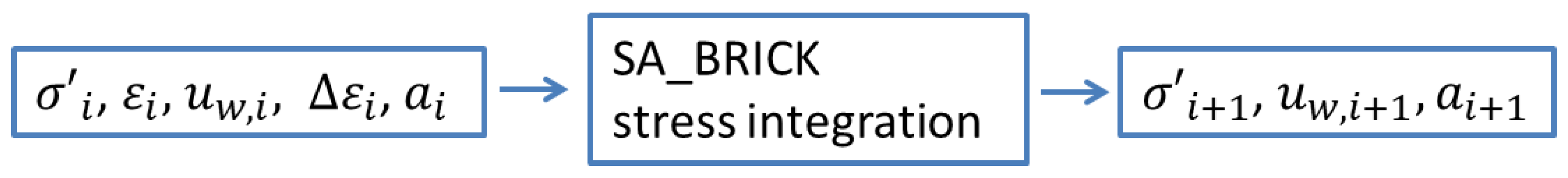
The main model input variables at the beginning of each step of loading in the global Newton–Raphson iteration are stress , strain , pore pressure , state variables , as well as the iterative strain increment . According to the given iterative strain increment coming from the main PLAXIS core routine, the implemented model integrates the stresses , pore pressure and state variables at each iteration which represent the output variables, as schematically presented in Figure 6 for the SA_BRICK model. The stress integration is performed by applying the strain increment Δεi on the current setting of bricks in strain space while running algorithms to iteratively move bricks and accumulate stresses along the elastic strain increments. In this procedure the proper string lengths must be considered along with all the changes of the state variables and iterative corrections. More details on BRICK implementation can be found in [17,44], while the use of PLAXIS user-defined soil models can be found in [19].
4. Validation of the SA_BRICK Model
4.1. Verification of the Modelling of Anisotropy
A series of numerical calculations were carried out using the single finite element program NAPGeo and the SA_BRICK model to investigate the behaviour of London clay under different stresses and types of loading conditions. These predictions were directly compared against the results of high-quality laboratory triaxial tests, which were undertaken as part of several doctorate research projects [47,48] and also [18,28].
In order to check the validity of the introduction of anisotropy in the SA_BRICK model, the first comparison was made with the results of the validation of the anisotropic model A_BRICK. In his research, Ellison [45] used samples tested by Nishimura [48] from the units C and B2, that is, samples labelled 7.2UC and 7.2UE, and by Gasparre [47], i.e., samples 10.1UC and 10.2DE, taken from the Terminal 5 site at London’s Heathrow Airport. The number indicates the depth from which the sample was taken, and the symbol indicates whether it was a triaxial drained (D) or undrained (U) investigation under compression (C) or tension (E) conditions. The modelling considered the geological history of the location from which the samples were taken. This initial stress path was followed by the unloading caused by sampling, and after the establishment of the initial stress state through isotropic compression, a shearing in compression or extension was modelled. A detailed explanation of the validation modelling procedure will be given in the next section.
For the sake of comparability, the same geological history and the same sample stress paths were used in the laboratory in this research as in the analysis provided by Ellison [45]. It should be observed that when discretizing the S-curve, Ellison adapted string lengths to fit the stiffness degradation curves determined for London clay by Gasparre [47]. In this type of verification of SA_BRICK, identical input parameters as in [45] were used, along with the anisotropy, which was taken into account from the very beginning, i.e., already during the course of sedimentation.
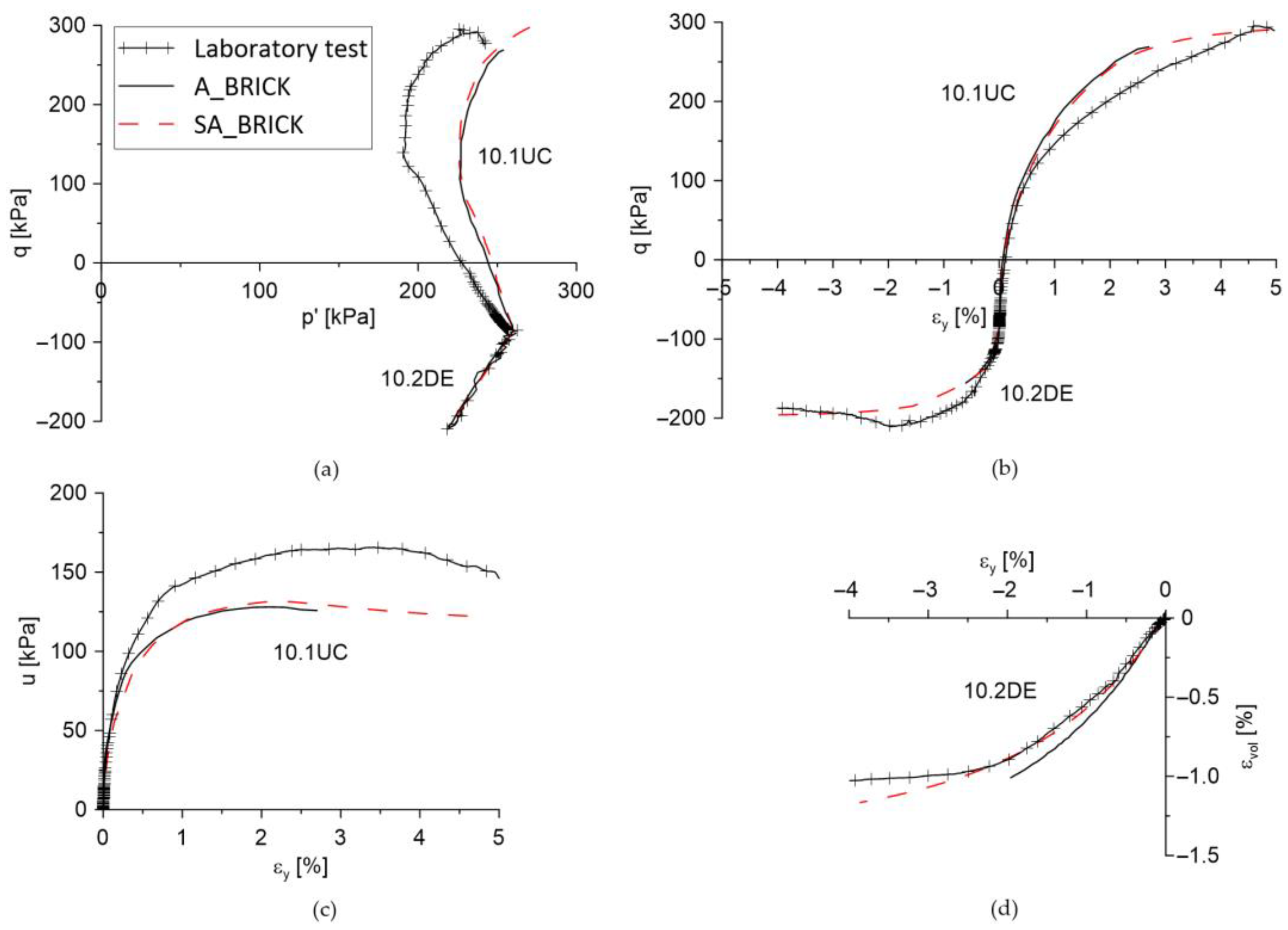
The SA_BRICK model results are given in Figure 7, together with the prediction of the A_BRICK model and the laboratory results (labelled LAB). The results are shown for samples 10.1UC (undrained shear in compression; upper part in all diagrams except 7d) and 10.2DE (drained shear in extension; lower part in all diagrams) showing the q–p′ diagram, q–εy diagram, u–εy diagram, and εy–εvol diagram (only for drained sample 10.2DE). Verification data of the A_BRICK model on London clay samples do not allow a comparison of stiffness, as they are not given in Ellison’s work. It can be seen in the figure that the modelling of anisotropy in SA_BRICK is fully comparable with the results in [45] for both cases, as SA_BRICK gives practically the same results as the A_BRICK model. A partial deviation is visible only in the case of volume deformation prediction (Figure 7d). It should be noted that the laboratory test 10.1UC (upper part in diagrams) was undrained so that the effective stress paths in the laboratory were driven by the changes in pore pressures. As it can be seen in Figure 7c, this change was underestimated by both the A_BRICK and SA_BRICK model, so it was impossible to model the stress path exactly. In the drained test 10.2DE, this was not the issue, so the stress path was fully matched. Certain minor deviations can also be attributed to the different steps for the load steps, the position or placement of the initial bricks and strings, and the accuracy of the given geological history and sampling.
4.2. Calibration of the SA_BRICK Model against the Results of Laboratory Testing on the Samples of Natural London Clay
As already mentioned, Ellison [45] did not use the string lengths suggested by Simpson [8] in discretizing the S-curve, but adapted them to fit the stiffness degradation curves determined for London clay by Gasparre [47]. This was understandable, as there was no attempt to model the structure. In the formulation of the SA_BRICK model, a different approach was taken so that the string lengths determined by Simpson [8] were treated as model parameters and were not changed. Instead, the effect of structure on the stiffness degradation S-curve was implemented, using the parameter by Vukadin and Jovičić [16], as explained in the previous section.
Table 3 provides basic input data for SA_BRICK model. Parameter values for anisotropy are taken according to [44] and did not change during the analysis. The parameters λ and κ for London clay were determined on the basis of oedometer tests [47]. The length of the strings was modified by the factor fSL = 0.8, which corresponds to a basic angle of shearing resistance of 20.5°. To model the structure, the laboratory results were best characterized by the value α = 1.2 for the strength, and by the value of ω = 0.85 for the stiffness. Anisotropy parameters were accepted after [44], with parameter υhh approximated as zero, as previously taken by other researchers [42,49].
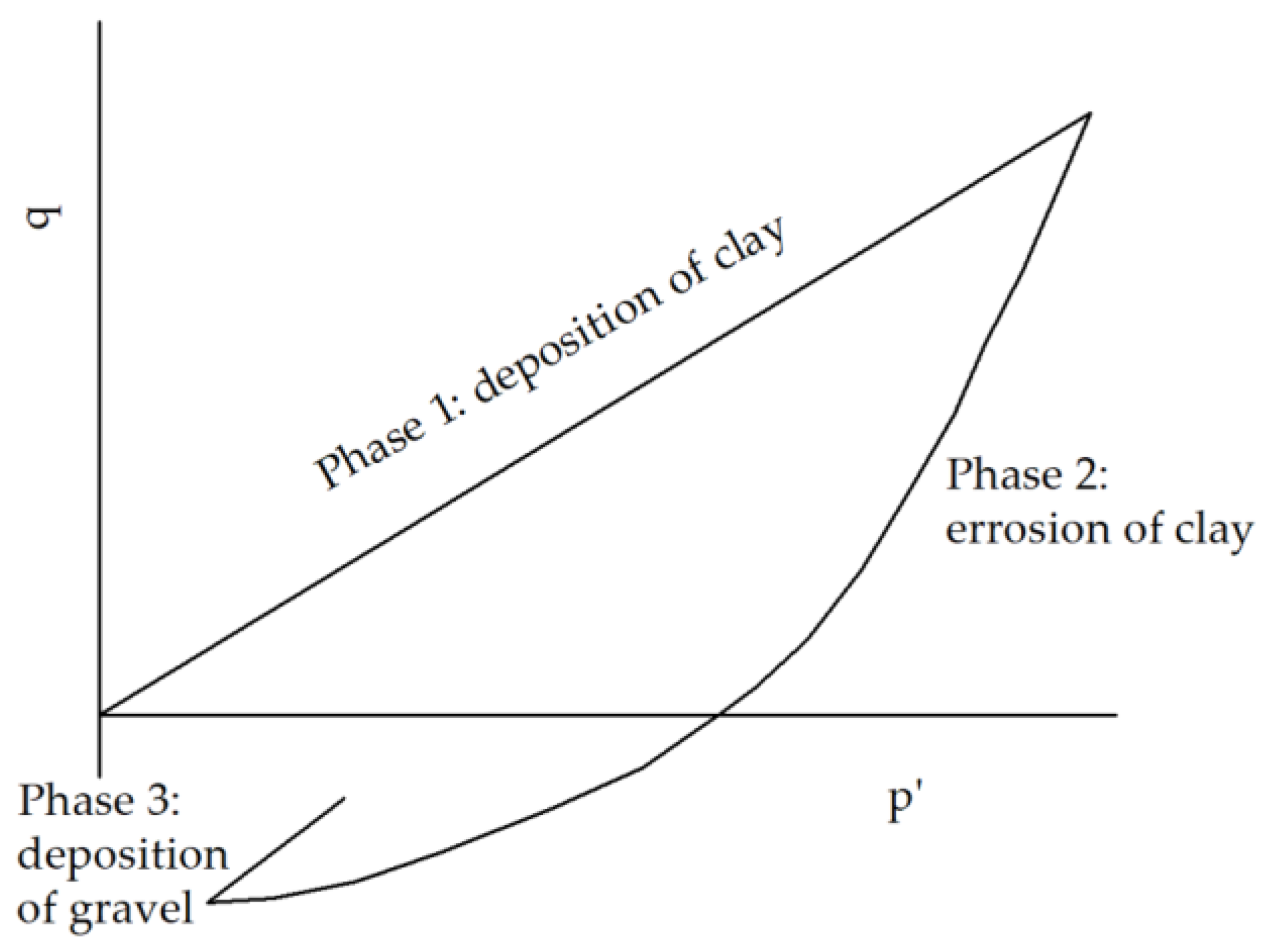
Geological history was evaluated for the given site of Heathrow Airport Terminal 5 [26,47], from where the samples were taken. Generally, the modelling of geological history included the deposition of clay (sedimentation) and the erosion of 175 m of London clay, which was followed by the subsequent deposition of 6 m of gravel (Figure 8). Both structure and anisotropy were modelled after the end of sedimentation and before erosion, which was then followed by the deposition of gravel. Modelling of geological history was followed by the unloading caused by sampling, and after the establishment of the initial stress state through isotropic compression, the exact stress path (e.g., shearing in compression or extension) was modelled as in the triaxial test as used by Gasparre [47].
In this research, the samples from lithological unit B2a were chosen for the analyses. The intention was to be compatible with the depth of excavation of the twin tunnels under St. James’s Park, the modelling of which will be explained in the next section (the tunnel tubes are located at a depth of between 20 and 30 m).
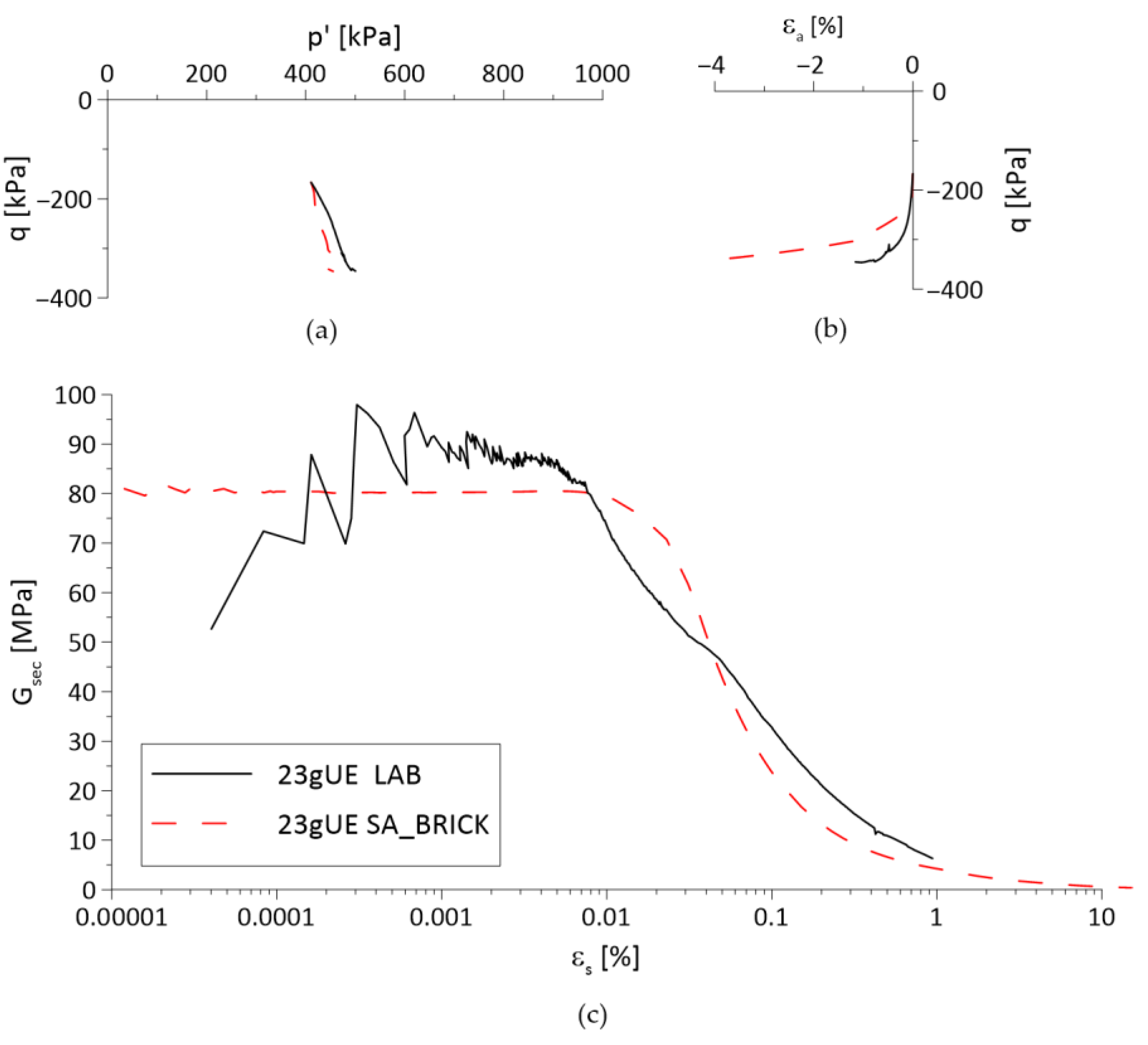
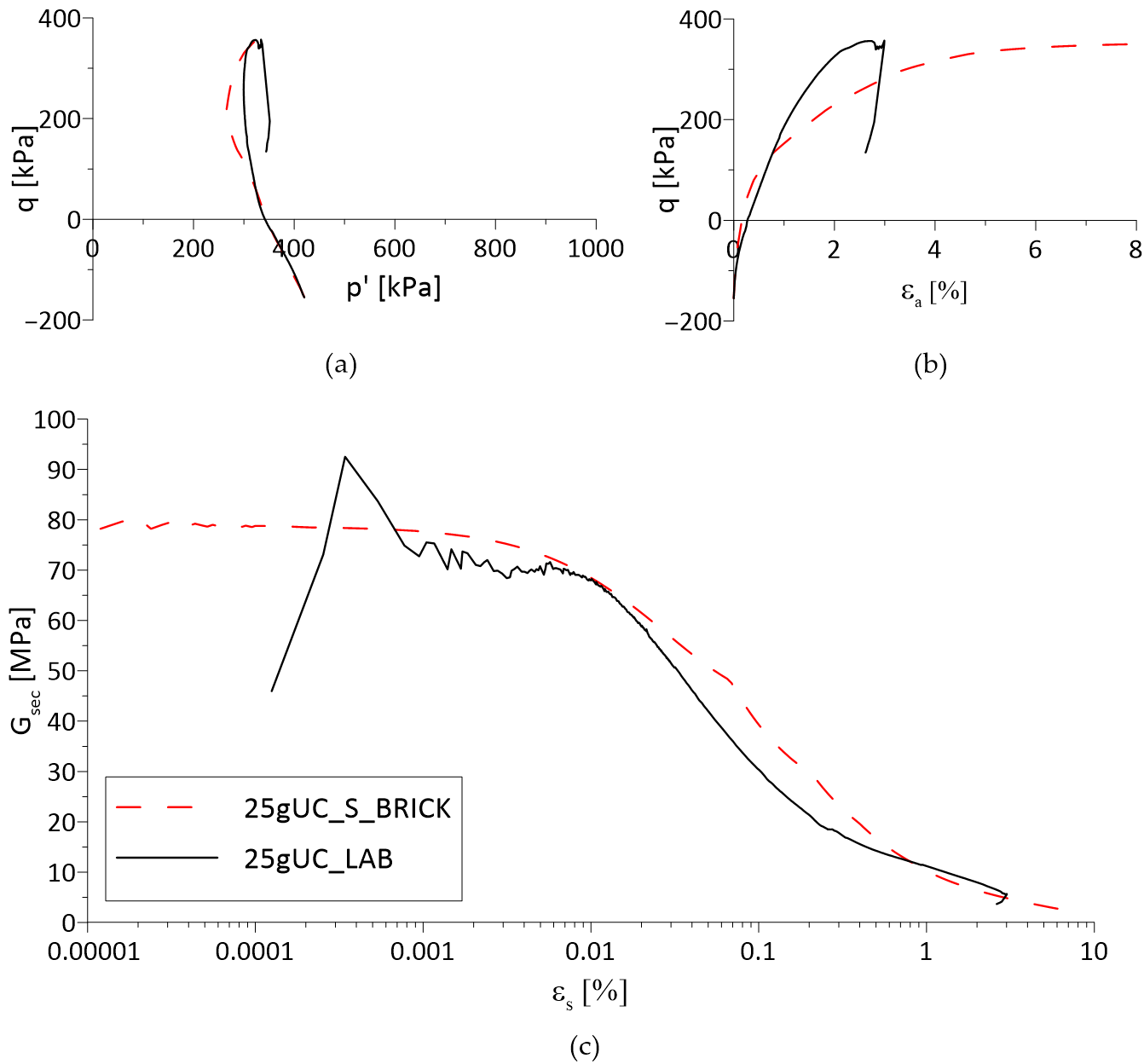
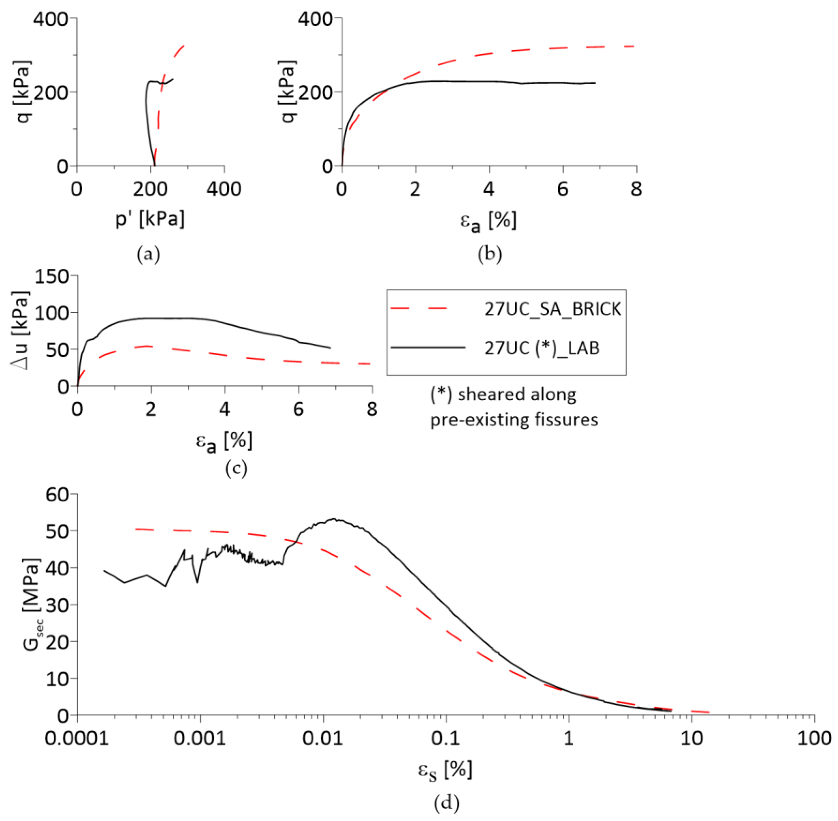
The validation results on samples from unit B2a are shown in Figure 9 and Figure 10. Each figure contains three diagrams: q–p′ diagram, q–εa diagram and Gsec–εs diagram so that important aspects of mechanical behaviour can be evaluated. Figure 11 additionally contains a Δu–εa diagram, since the measurements of pore pressure were available for this test. Figure 9 shows the validation results of the SA_BRICK model on samples 23gUE (undrained extension), while Figure 10 shows the validation results of sample 25gUC (undrained compression), and Figure 11 validation on sample 27UC (undrained compression).
A good agreement can be observed between the modelled and measured data in all diagrams. All aspects of the mechanical behaviour of the tested samples are within reasonable limits, covering both compression and extension shearing. Generally, in undrained tests, effective stress paths in the laboratory were driven by the changes in pore pressures. This change was underestimated by the SA_BRICK model so there was no possibility to model the stress path exactly (e.g., Figure 9a and Figure 10a), which was reflected at large strains so that the absolute value of the maximum deviator stress qmax was almost exactly matched but twice as large as the axial strain εa (e.g., Figure 9b and Figure 10b). The sample 27UC (Figure 11) was sheared along pre-existing fissures which was reflected again at large strains so that the prediction of qmax was about 50% larger that the measured value.
In particular, a good agreement was observed in the area of small strain behaviour, that is, for the shear strains within the region 0.0001% to 0.1%, in which elastic plateau was modelled within the 10% margin. These results enabled a next stage in this research, which was the modelling of the tunnel excavations in London clay, which will be explained in continuation.
5. Analyses of the Settlement Trough
5.1. Modelling of the Excavation of the Jubilee Line Tunnels at St. James’s Park
The tunnels under St. James’s Park (London, UK) were built in 1996 as part of the Jubilee line metro extension project. This boundary value problem in London clay was chosen with an aim of using high-quality observation data which were unaffected by urban development. South of the lake in St. James’s Park, an instrumented greenfield monitoring section had been set up, based on which the analyses of the monitoring data were carried out by Nyren et al. [20]. The monitoring system and the precise measurements of the settlement trough caused by the excavation of the Jubilee Line tunnels were comprehensively presented by Standing and Burland [27].
Finite element programs ICFEP [50] and PLAXIS [19] were both used to carry out a series of numerical analyses with an aim of comparing predictions of displacements around the mentioned tunnels. In the program ICFEP, the models M2-SKH and M3-SKH were used, while in PLAXIS, the BRICK and SA_BRICK models were used. The purpose of the use of more kinematic hardening models was to make a comparative analysis of the accuracy of the model predictions.
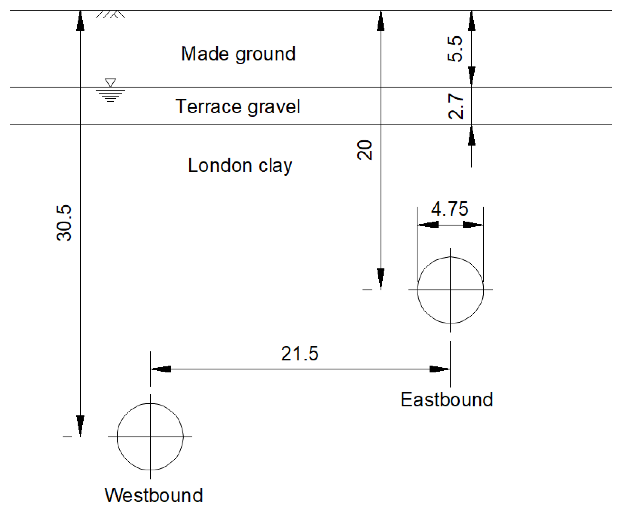
The geological profile with the geometry of the tunnels is shown in Figure 12. The profile consists of a 5.5 m thick made ground and alluvium, under which there is 2.7 m of Terrace gravel underlaid by some 35 m thick layer of London clay, below which is a base of hard Lambeth Group Beds. The groundwater was immediately above the gravel layer. The diameter of the tunnels excavated at 20.0 m (east tube) and 30.5 m (west tube) depths was 4.75 m. The west tube was built first, followed by the east tube some eight months later. The tunnels were excavated using a TBM of open-faced type with a 4.2 m long shield, while face excavation was carried out by a back-hoe machine. The precast concrete linings were installed behind the shield after thrusting ahead off the previously constructed ring.
Excavation of the two tunnel tubes under St. James’s Park took place in undrained conditions and was modelled accordingly using the “volume loss” method. It should be noted that the term “volume loss” is not strictly technically correct as there is no change in volume in undrained conditions. It is used to indicate a part of the volume change caused by the convergence movement of tunnel excavation, which is compensated for by the subsidence of the terrain on the surface. Thus, the volume of material converging to the tunnel cavity (Vl) is equal to the volume of deformation that appears as settlement on the terrain surface (Vs). The excavation of the tunnel is modelled in small excavation increments, while the installation of the tunnel lining is simulated at the point in which the prescribed value of the volume loss is achieved. The use of the “volume loss” method in finite element analyses is detailly described in [50].
The presence of groundwater was also considered at a depth of 5.5 m, as indicated in Figure 12. The hydraulic boundary conditions were determined as drained conditions for two upper layers (made ground and gravel), while the pore pressures were assumed to be constantly increasing along the boundaries of London clay. In the ICFEP program, the initial stresses, the pore pressures, and the coefficient of horizontal pressure at rest K0 values were defined at the beginning of the analyses, as a separate input file. Models with kinematic hardening M2-SKH and M3-SKH enable the modelling of geological history, but geological history was not included in the analyses. Instead, the focus was on the adequate K0 profile, which means that there were kinematic surfaces centred prior to the modelling of the excavation of the tunnel.
The input data for the M2-SKH model and the M3-SKH model were determined based on simulated undrained triaxial laboratory tests. The aim was to determine the parameters that most adequately describe the stiffness degradation obtained in the laboratory. It should be noted here that the existing experimental data did not include stress paths that would allow the calculation of the parameter T (ratio of the size of the history surface relative to the size of the bounding surface), so it was determined based on values given by Grammatikopoulou [51]. Due to this uncertainty, two sets of input data were used to encompass a range of reliable input data. These were named “previous soft” and “new data” to retain the same notation as in [52]. It should be noted that “previously soft” data refer to a softer response of laboratory samples and that exclusively “new data” were used for validation of the SA_BRICK model. For comparison purposes, we provide the full set of input parameters for M2-SKH and M3-SKH models that were used in ICFEP analyses in Table 4 [52].
The programs PLAXIS and ICFEP differ in the form of the elements that can be generated in the finite element mesh. To achieve comparability of the number of Gaussian points in both programs, the triangular finite elements with 15 Gaussian points were used for calculation in the PLAXIS program. The input parameters for the BRICK and SA_BRICK models are given in Table 1 and Table 3, respectively.
To initiate the models, it was necessary to determine initial stresses and states by calculating the positions of strings and tension states of bricks prior to the excavation of the tunnel. These were determined using the single-element NAPgeo program by simulating the geological history up to the point of sedimentation for the same input parameters. State values, string position and the stress states were further copied to a separate file which was used as an input to start the PLAXIS analysis. The geologic history was further modelled assuming an additional thickness of 175 m of London clay above the existing profile, which was removed gradually, so that up to 20 m of clay was removed in each step to mode erosion. Apart from the mesh generation, the PLAXIS and ICFEP programs also differ in the method of modelling the excavation tunnel and lining placement. However, the program PLAXIS enables automatic modelling of the installation of the lining after a previously determined percentage of volume reduction, which is an equivalent procedure the “volume loss” method.
In both PLAXIS and ICFEP analyses, made ground and gravel deposits (terrace gravel) were modelled using the Mohr–Coulomb model and the input parameters given in Table 5.
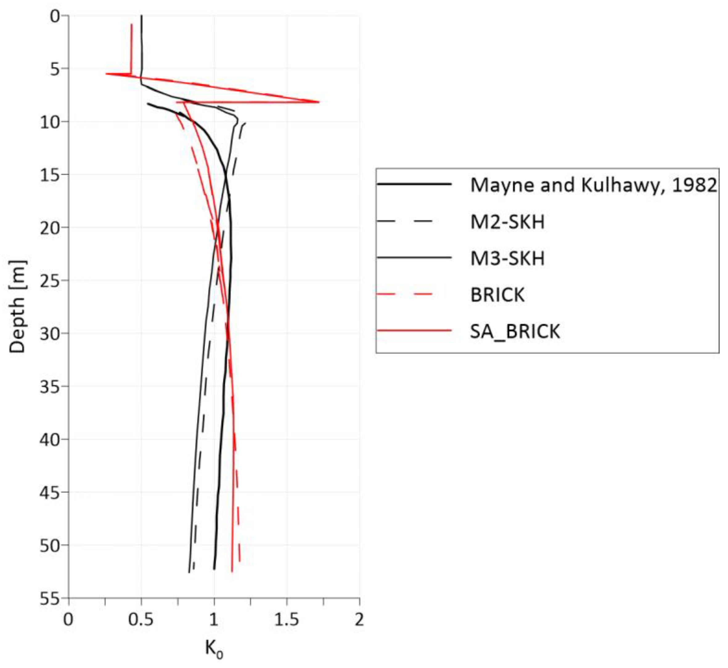
Apart from the effect of anisotropy [42,53,54], the prediction of deformations in overconsolidated soils, such as London clay, is highly dependent on the initial horizontal pressure at rest K0, as highlighted in previous numerical studies (e.g., [55,56]). It was, therefore, necessary to check the predictions of the K0 profile for all the models used prior to the modelling of tunnel excavation. The predicted K0 profiles for the models BRICK and SA_BRICK are shown in Figure 13 along the prediction curves of M2-SKH and M3- SKH obtained for the same profile [51]. As a reference, the prediction based on empirical correlation of Mayne and Kulhawy [57] for overconsolidated clays is also presented in the same figure.
It can be seen in Figure 13 that despite different approaches, the K0 profiles are in good agreement for all four models used. It should be observed that at the depths of tunnel excavations (e.g., between 20 m and 30 m), the values for K0 are close to 1.0 for all model predictions, including the empirical approach.
5.2. Results and Interpretation of the Analyses
5.2.1. Modelling of the Excavation of the West Tube
A particular feature of the analyses is the modelling of the high percentage of volume loss recorded during the excavation of the tunnel, which was 3.3% for the west tube and 2.9% for the east tube. This was a much higher volume loss than expected, which on average for London clay is between 1.0 and 2.0% [58], where a 2% is regarded a conservative estimate.
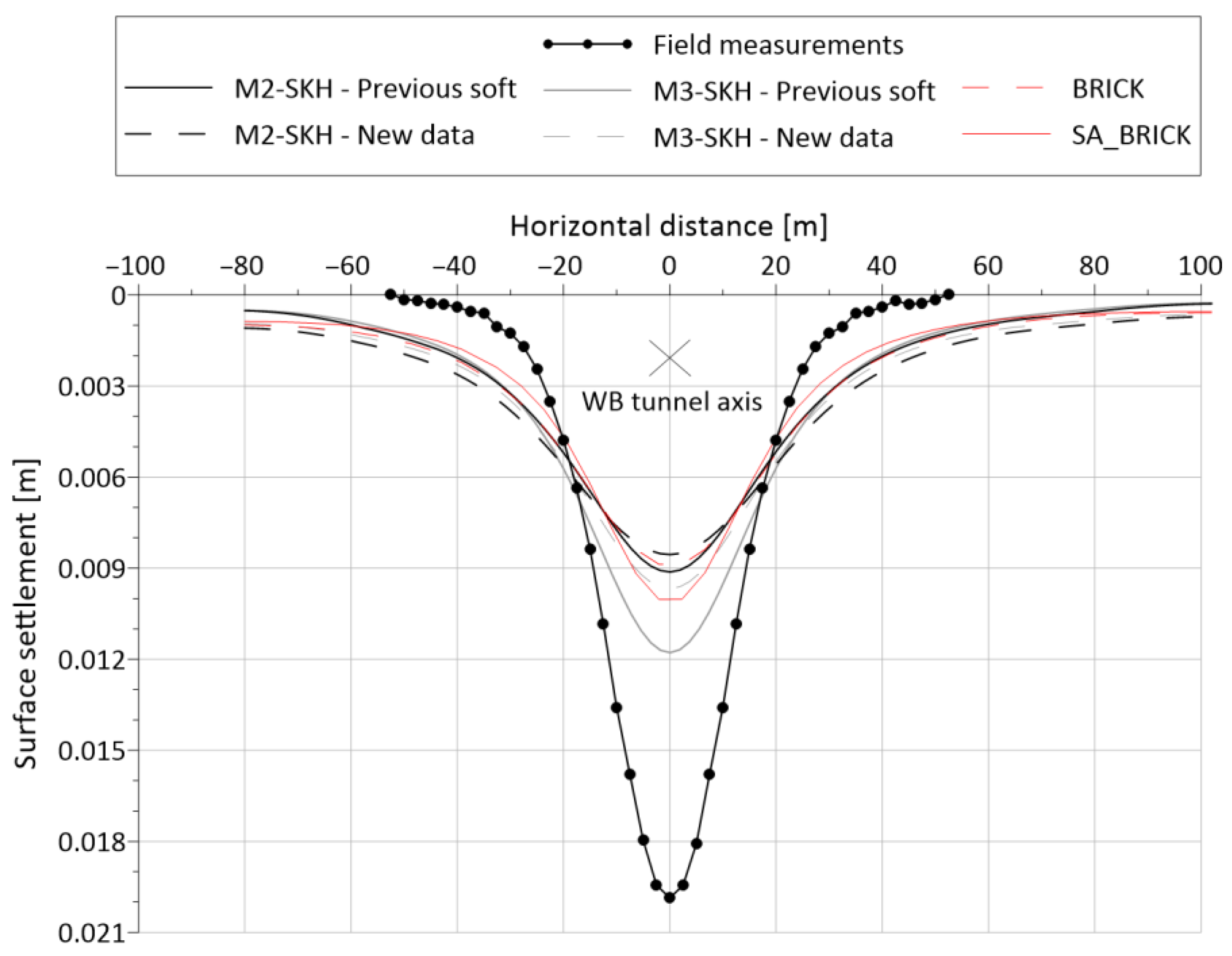
The results of modelling of the excavation of the west tube using all four kinematic hardening models are shown in Figure 14 and the annotated field data was taken from [27]. All the graphs are shown relative to the axis of the west tube, which was excavated first. It can be seen in the figure that the largest settlements of 11.2 mm are predicted by the M3-SKH “previous soft” model. The SA_BRICK model predicts settlements of 10 mm while the BRICK model predicts those of 8.9 mm. However, the maximum measured settlement [20], labelled as field data, was for the west tube in excess of 20 mm, which was much higher than expected. Standing and Burland [27] attributed the causes of excessive volume loss to the fact that up to 1.9 m of unsupported tunnel heading was often advanced ahead of the shield, and as a result, about 50% of the measured volume loss occurred in front of the shield. They also commented that this division of the London clay contained sand and silt partings, giving potential for loosening and softening above the tunnel and well ahead of the shield. As indicated by Dai at al. [59], instabilities in the shield excavation can be also significantly affected by the anisotropy of soil strength on ultimate supporting force, which can be also a cause of increased volume loss.
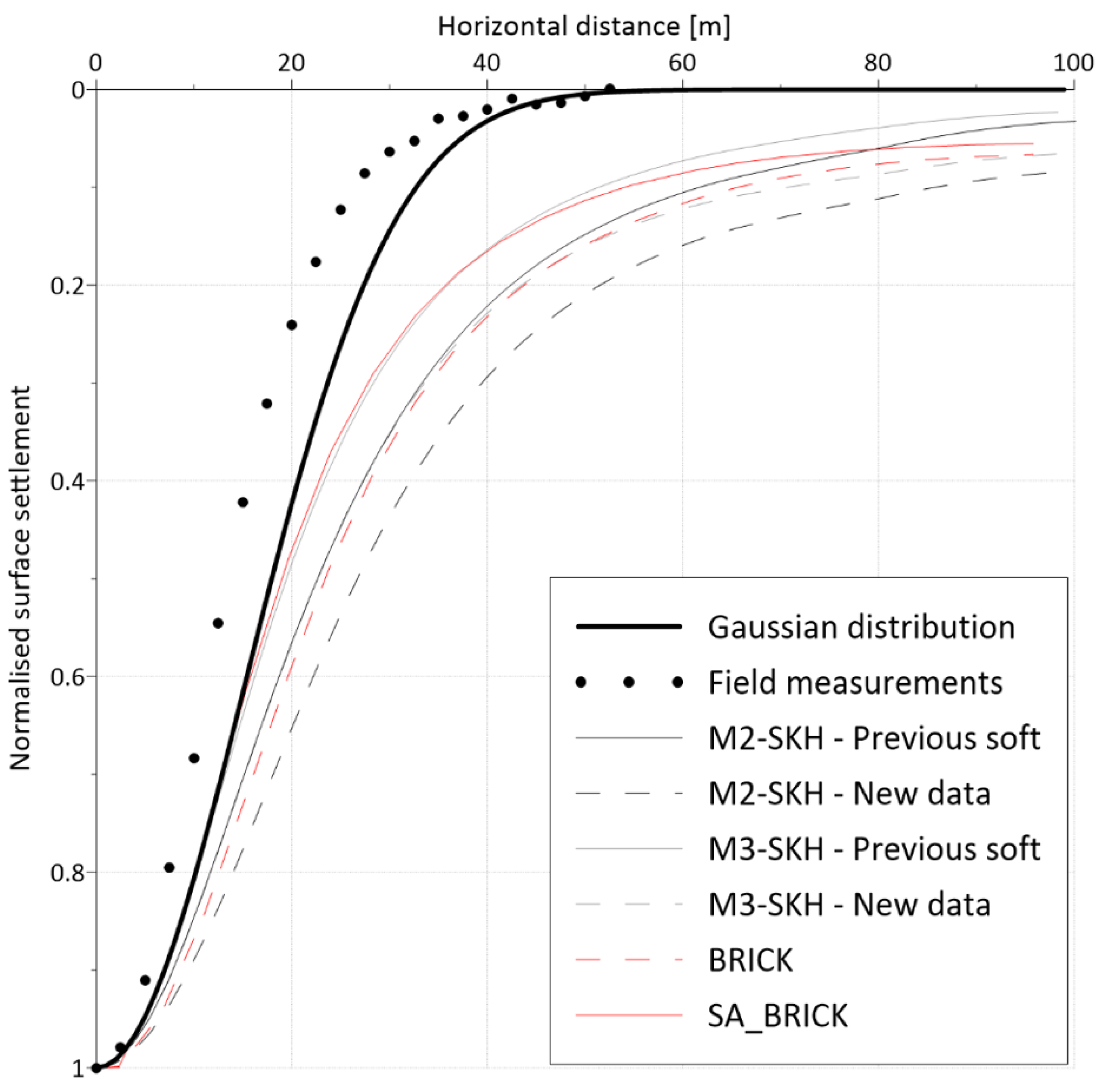
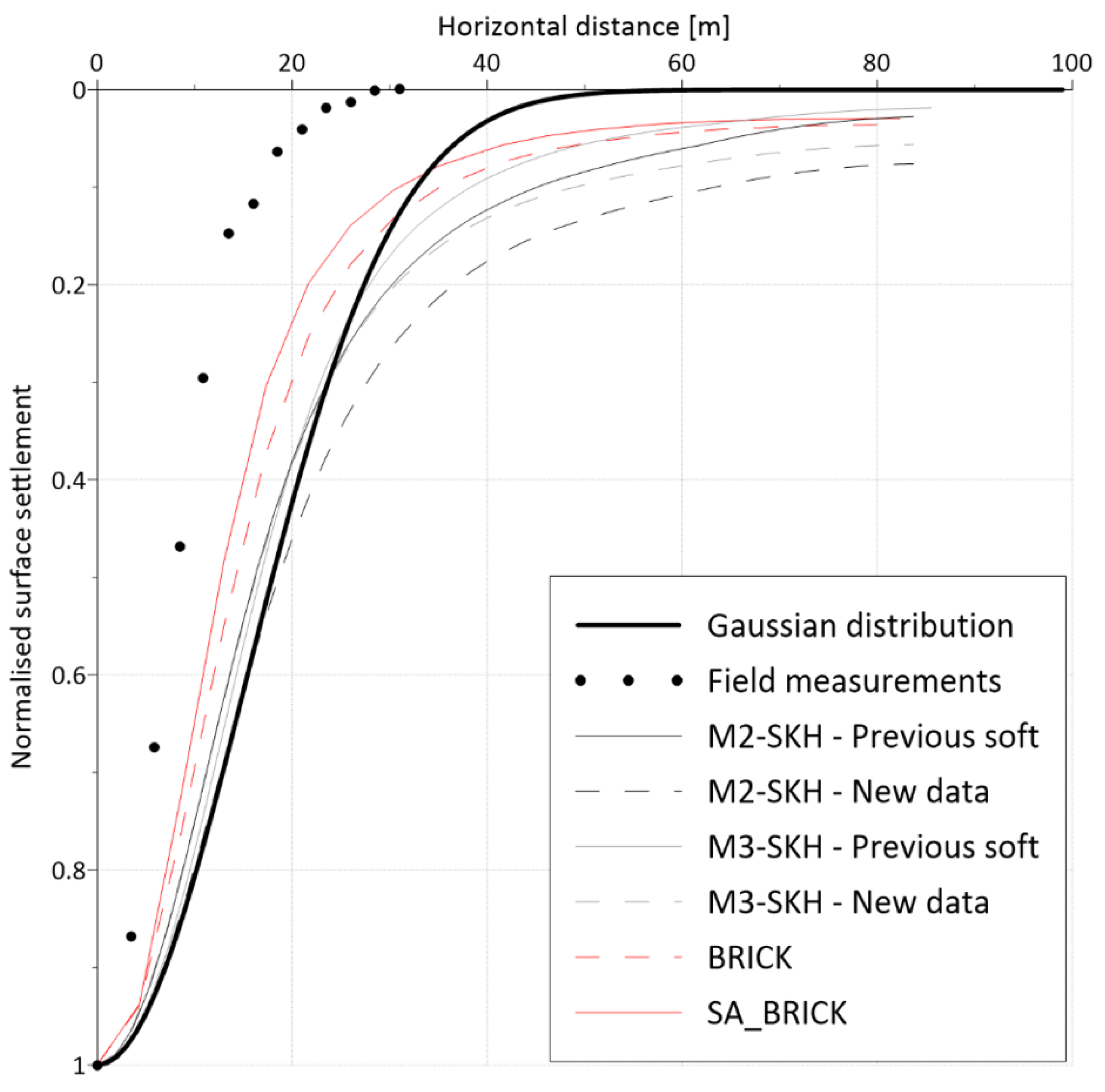
In terms of the accuracy of the prediction, the normalized graphs give a better representation of the narrowness of the settlement trough, which is the critical parameter for the possible impact of the tunnel excavation on the structures on the surface [60]. The normalized curves are, in practice, compared with the Gaussian distribution, which is widely accepted as a reference empirical curve [61], giving a fairly accurate general representation of the magnitude and lateral extent for the settlement trough.
The vertical movements, normalized by the maximum settlement of the individual analysis are shown in Figure 15 together with the Gaussian distribution and the normalised settlement measured on the site. It can be seen in the figure that the Gaussian curve is the most approximate, with the prediction of SA_BRICK and M3-SKH as “previous soft”, but both still deviate from the field models measurement. It should be noted that the SA_BRICK model was calibrated against “new data” which illustrate a much stiffer behaviour and not “previous soft” as M3-SKH in this case.
There is also a distinctive difference between the prediction of the BRICK and SA_BRICK models, in which the SA_BRICK model gives a much narrower settlement trough. This result substantiates the appropriate choice of parameters and adequate implementation of both structure and anisotropy in the SA_BRICK model. Apart from that, it can be observed that the field data give a much narrower settlement trough than the Gaussian distribution curve. As already discussed, this fact is attributed by Standing and Burland [27] to an unexpectedly high volume loss at this section of the tunnel.
5.2.2. Modelling of the Excavation of the East Tube
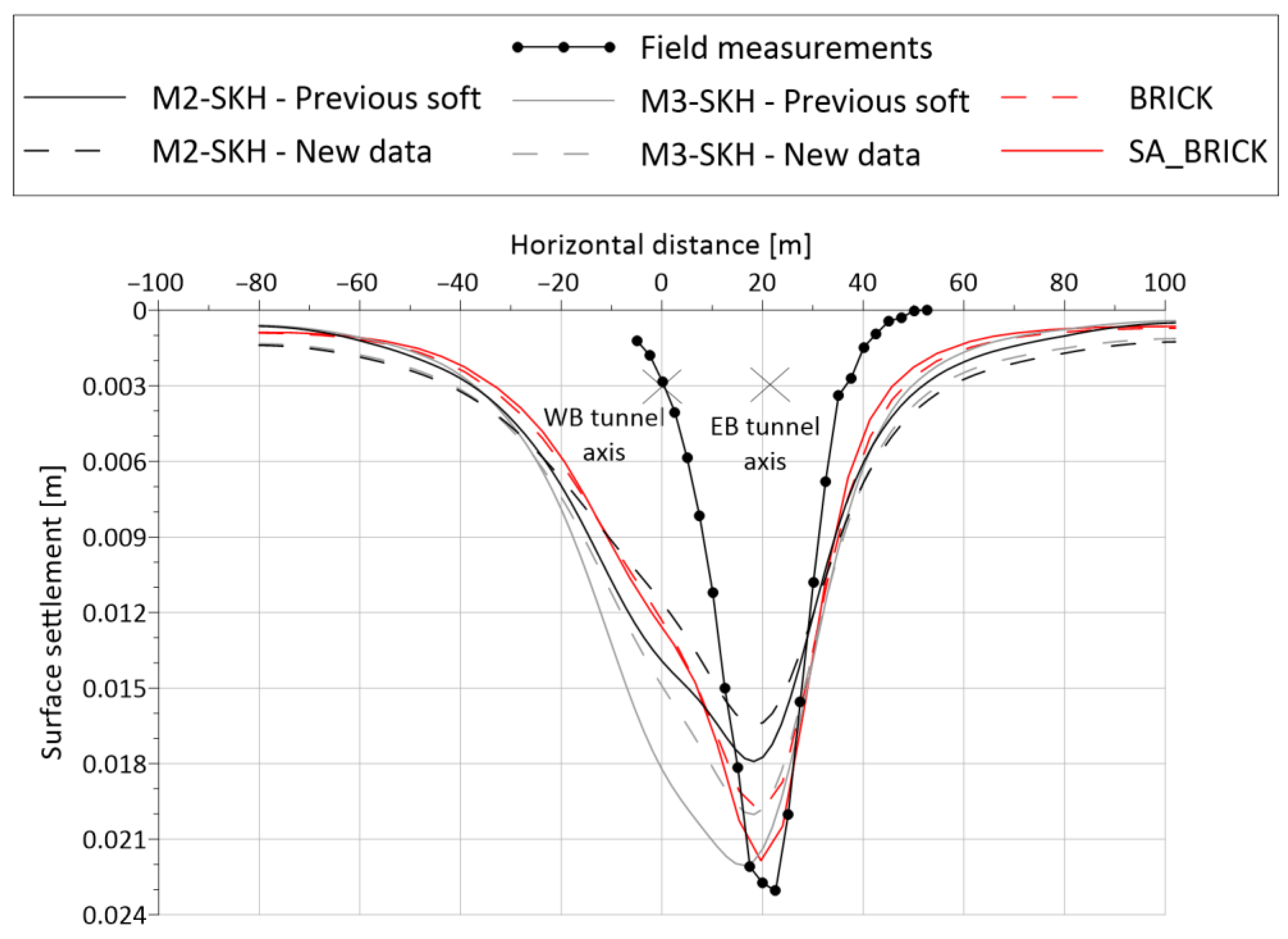
The settlement trough formed during the construction of the east tube (total settlements since the construction of both tunnel tubes including an 8-month delay period between the construction of the west and east tube) is shown in Figure 16. It can be observed that the settlement trough moves to the right so that is above east tube axis and that the measured settlements are in good agreement with the calculated settlements on the side of the east tube. As expected, the discrepancies between measured and calculated movements above the west tube also persisted in this analysis. Among the predictions of the other kinematic hardening models, the results of the SA_BRICK model are in the best agreement with the measured data on the east side of the settlement trough. Additionally, the SA_BRICK model gives a more accurate prediction of the maximum settlement compared to the BRICK model.
In comparison to the west tube analyses, a better accuracy of prediction could be attributed to the fact that volume loss for the excavation of the east tube was lower so that the total magnitude of displacement of 24 mm is in very good agreement. The analyses also predicted the impact of the ground disturbance initiated by the excavation of the west tube well, which is seen in the asymmetry of the trough. As observed by Standing and Burland [27], a volume loss of 2.4% might be taken as a plausible estimate for the initially undisturbed ground for the construction of the east tube. This is much closer to the expected quantities of volume loss in London clay [58], so the numerical analyses were within the range of expected ground behaviour and gave better predictions.
Finally, the vertical movements, normalized by the maximum settlement of the individual analysis for the east tube are shown in Figure 17 together with the Gaussian distribution and the normalised settlement measured on the site. In this case, all the predictions give narrower settlement troughs than the Gaussian distribution as they include the superposition of the excavation of both tubes, while the Gaussian curve can account for one tube only. Again, it can be observed that the SA_BRICK model best predicts the narrowest settlement trough in this case, followed by the BRICK model.
6. Discussion
An overview of the development and validation of a constitutive model SA_BRICK is presented in the paper. The SA_BRICK model is a continuation of the development of the BRICK model which was initially developed by Simpson [8] for overconsolidated clays. The SA_BRICK model was created on the basis of the extended S_BRICK model [16] by including a variation in the modelling of soil structure. It was further improved by adding the ability to model anisotropy, as developed by Ellison et al. [44] for the basic BRICK model.
All the above-mentioned features of the mechanical behaviour of natural soils are found in London clay, which was used as a prototype material in this research to the check applicability of the SA_BRICK model to simulate tunnel excavation in London clay. By using high-quality laboratory data [47,48], the model was calibrated to define the unique selection of input parameters. The calibration considered the geological history of the location from which the samples were taken, and the full modelled stress path in the laboratory to include unloading caused by sampling, and shearing in compression or extension, as appropriate. The validation of the model was carried out for samples originating from three different London clay units and a good agreement was achieved. Generally, the data on small strains were in better agreement with the laboratory results in comparison to the behaviour at large strains. This was attributed to the fact that several samples failed in the laboratory on pre-existing fissures, the modelling of which was beyond the scope of the research. This feature does not affect the overall conclusions of the numerical analyses as the field measurements of the displacements of the tunnel excavation were in the small-strain region.
Calibration of the SA_BRICK model was carried out by using a purpose-developed single finite element program NapGeo. Once the model was checked and calibrated in NapGeo, it was automatically set to be used for numerical analyses of tunnel excavation which were carried out in finite element program PLAXIS. This approach enables the development and calibration of numerical models in single-element form and easy transition to the validation procedure on real size boundary value problems using already developed finite element software.
By applying the above-described methodology, the SA_BRICK model was used to carry out “Class C1” [62] analyses to predict ground behaviour caused by the excavation of the Jubilee Line tunnels at St. James’s Park in London. The prediction of the model was checked against the predictions of other kinematic hardening models, denoted M2-SKH [7] and M3-SKH [13,51], and the basic BRICK model [8]. The analyses using M2-SKH and M3-SKH models were carried out using the finite element program ICFEP [50], while the analyses using the BRICK and SA_BRICK models were carried out using PLAXIS [19]. Particular care was taken to apply equivalent numerical procedures for modelling in ICFEP and PLAXIS to achieve comparable results. In particular, the initial stress state and the modelling of geological history of the site were carefully adjusted so that the numerical analyses of the tunnel excavation could be carried out using matching boundary conditions, including the K0 distribution. The thorough approach was used to compare two different calculation engines (i.e., ICFEP and PLAXIS) in analysing the same boundary value problem. Sound agreement between the two sets of results confirmed the suitability of the used methodology and the high reliability of both software packages. This confirms that kinematic hardening models can provide comparable and compatible results based on the same sound theoretical background, regardless of the mathematical formulation (e.g., BRICK versus 3-SKH model) and numerical tools used, if they are founded on correct formulation of the parameters derived from the high-quality laboratory testing. In that sense, the improvement made by SA_BRICK by accounting for the anisotropy and structure versus the 3M-SKH model is notable.
7. Conclusions
With the further development of the built environment, the accurate numerical prediction of the deformation field around a tunnel excavation becomes increasingly important as more traffic routes require the use of underground space. Predictions of ground deformations caused by tunnel excavations with increased accuracy are important to assess, prevent, and mitigate possible damage of existing structures caused by tunnelling. It was demonstrated in the paper that the SA_BRICK model can be used to advance numerical modelling of such boundary value problems with increased accuracy.
Based on the good agreement between laboratory results and numerical predictions, it can be concluded that the SA_BRICK model presents a complete kinematic hardening model by exhibiting the ability to model the main manifestations of the mechanical behaviour of natural clays, including the non-linear stress–strain response of soil, the recent stress history effect, the effect of structure, and the effect of anisotropy. In addition to London clay, the model SA_BRICK was successfully validated against the behaviour of other natural soil, i.e., Pappadai clay, as demonstrated by Jurečič [63] and Jurečič et al. [64].
Numerical analyses of the excavation of the Jubilee Line tunnels at St. James’s Park comprised modelling of the west and east tube. For the modelling of the west tube, all kinematic hardening models predicted a maximum settlement of some 10 mm, which was twice less than that observed. This discrepancy was attributed [27] to excess unsupported tunnel heading and to local geological conditions affected by sand and silt partings giving potential for loosening and softening above and in front of the tunnel heading. However, when comparing the normalized data of the predicted settlement trough with the Gaussian distribution, the prediction of the SA_BRICK and M3-SKH models were the most accurate. In particular, a distinctive difference of the SA_BRICK model giving a much narrower settlement trough than BRICK was observed. It should be noted that the SA_BRICK model was calibrated against “new data”, which, in comparison to the M3-SKH model, illustrated a much stiffer behaviour of soil.
In the modelling of the east tube, the SA_BRICK model gives the most accurate prediction of the settlement trough in comparison with other models and is in fair agreement with the observed data. This is attributed to the fact the east tube was excavated in initially undisturbed ground, so that the numerical analyses were within the range of expected ground behaviour and gave better predictions overall.
Finally, it can be concluded that the results presented in this research demonstrate that the main features of the behaviour of natural overconsolidated clays can be captured reasonably well to include the effects of structure and anisotropy by following a thorough and comprehensive process of the development of the kinematic hardening model and the appropriate calibration of input parameters. When compared to other kinematic hardening models, the improvements in SA_BRICK predictions presented in this paper confirm the adequate implementation of structure and anisotropy in the BRICK model, which resulted in more accurate and realistic simulations of the mechanical behaviour of a natural overconsolidated clay. The obvious advantage of the SA_BRICK model is completeness of the phenomena that can be accounted for to model the behaviour of natural clays using a single formulation. As a superposition of BRICK, A_BRICK and S_BRICK, the SA_BRICK model contains all the previous phases of the BRICK development and can be used for modelling a wide area of soils. As for the other kinematic hardening models, the preconditions for the appropriate use of the SA_BRICK model are high quality laboratory data needed for the selection of input parameters. This can be regarded as a disadvantage for a routine use of numerical analyses, but it also highlights a necessity for the further improvement in the laboratory and in situ testing to advance the characterization of natural clays.
Author Contributions
Conceptualization, N.J. and V.J.; methodology, V.J. and N.J.; software, G.V.; validation, N.J. and V.J.; formal analysis, N.J.; investigation, G.V. and N.J.; resources, V.J.; data curation, N.J., G.V. and V.J.; writing—original draft preparation, V.J.; writing—review and editing, V.J.; visualization, N.J. and G.V.; supervision, V.J. All authors have read and agreed to the published version of the manuscript.
Funding
This research received funding from the Public Agency for Research Activity of the Republic of Slovenia (ARRS) under the program “Young researcher”, Grant No. 1000-07-310074.
Institutional Review Board Statement
Not applicable.
Informed Consent Statement
Not applicable.
Data Availability Statement
Not applicable.
Acknowledgments
The authors express their gratitude to the Public Agency for Research Activity of the Republic of Slovenia (ARRS) for supporting scientific research, which is essential for the advancement of a knowledge-based society. The authors are thankful to Lidija Zdravković from Imperial College, London, UK for unreserved help and advice in running numerical analyses in the ICFEP finite element program. The authors would like to thank IRGO—Institute for Mining, Geotechnology and Environment, Ljubljana, Slovenia for material support to carry out this research.
Conflicts of Interest
The authors declare no conflict of interest. The funders had no role in the design of the study; in the collection, analyses, or interpretation of data; in the writing of the manuscript; or in the decision to publish the results.
References
- Simpson, B.; O’Riordan, N.; Croft, D.D. A computer model for the analysis of ground movements in London Clay. Géotechnique 1979, 29, 149–175. [Google Scholar] [CrossRef]
- Jardine, R.J.; Potts, D.; Fourie, A.; Burland, J.B. Studies of the influence of non-linear stress–strain characteristics in soil–structure interaction. Géotechnique 1986, 36, 377–396. [Google Scholar] [CrossRef]
- Mroz, Z.; Norris, V.; Zienkiewicz, O.C. An anisotropic hardening model for soils and its application to cyclic loading. Int. J. Numer. Anal. Methods Geomech. 1978, 2, 203–221. [Google Scholar] [CrossRef]
- Dafalias, Y.F. A bounding surface soil plasticity model. In Proceedings of the International Symposium on Soils under Cyclic and Transient Loading, Swansee, Wales, 7–11 January 1980; Volume 1, pp. 335–345. [Google Scholar]
- Al-Tabbaa, D.; Muir Wood, A. An experimental based ‘bubble’ model for clay. In Numerical Models in Geomechanics, Proceedings of the 3rd International Symposium, Niagra Falls, ONT, Canada, 8–11 May 1989; Pietruskzczak, A., Pande, G.N., Eds.; Elsevier: Amsterdam, The Netherlands, 1989; pp. 91–99. [Google Scholar]
- Atkinson, J.H.; Richardson, D.; Stallebrass, S.E. Effect of recent stress history on the stiffness of overconsolidated soil. Géotechnique 1990, 40, 531–540. [Google Scholar] [CrossRef]
- Stallebrass, S.E.; Taylor, R.N. The development and evaluation of a constitutive model for the prediction of ground movements in overconsolidated clay. Géotechnique 1997, 47, 235–253. [Google Scholar] [CrossRef]
- Simpson, B. Retaining structures: Displacement and design. Géotechnique 1992, 42, 541–576. [Google Scholar] [CrossRef] [Green Version]
- Cotecchia, F.; Chandler, R.J. A general framework for the mechanical behaviour of clays. Géotechnique 2000, 50, 431–447. [Google Scholar] [CrossRef]
- Leroueil, S.; Vaughan, P.R. The general and congruent effects of structure in natural soils and weak rocks. Géotechnique 1990, 40, 467–488. [Google Scholar] [CrossRef]
- Kavvadas, A.G.; Anagnostopoulos, M. A framework for the mechanical behaviour of structured soils. In Proceedings of the 2nd International Symposium on the Geotechnics of Hard Soils—Soft Rocks, Naples, Italy, 12–14 October 1998; pp. 603–614. [Google Scholar]
- Kavvadas, M.; Amorosi, A. A constitutive model for structured soils. Géotechnique 2000, 50, 263–273. [Google Scholar] [CrossRef]
- Baudet, B.; Stallebrass, S. A constitutive model for structured clays. Géotechnique 2004, 54, 269–278. [Google Scholar] [CrossRef]
- Gajo, A.; Muir Wood, D. A new approach to anisotropic, bounding surface plasticity: General formulation and simulations of natural and reconstituted clay behaviour. Int. J. Numer. Anal. methods Geomech. 2001, 25, 207–241. [Google Scholar] [CrossRef]
- Vukadin, V. Development of a Constitutive Material Model for Soft Rocks and Hard Soils. Ph.D. Thesis, University of Ljubljana, Ljubljana, Slovenia, 2004. [Google Scholar]
- Vukadin, V.; Jovičić, V. S_BRICK: A constitutive model for soils and soft rocks. Acta Geotech. Slov. 2018, 15, 16–37. [Google Scholar] [CrossRef]
- Ellison, K.C.; Soga, K.; Simpson, B. An examination of strain space versus stress space for the formulation of elastoplastic constitutive models. In Proceedings of the 7th European Conference on Numerical Methods in Geotechnical Engineering, Trondheim, Norway, 6 September 2010; pp. 33–38. [Google Scholar]
- Gasparre, A.; Nishimura, S.; Coop, M.; Jardine, R.J. The influence of structure on the behaviour of London Clay. Géotechnique 2007, 57, 19–31. [Google Scholar] [CrossRef]
- Brinkgreve, R.; Kumarswamy, S.; Swolfs, W.; Zampich, L.; Manoj, N.R. Plaxis Finite Element Code for Soil and Rock Analyses; Plaxis BV, Bentley Systems, Inc.: Philadelphia, PA, USA, 2019. [Google Scholar]
- Nyren, R.J.; Standing, J.; Burland, J.B. 25 Surface displacements at St James’s Park greenfield reference site above twin tunnels through the London Clay. In Building Response to Tunnelling; Thomas Telford Publishing: London, UK, 2001; pp. 387–400. [Google Scholar]
- Jardine, R.; Brosse, A.; Coop, M.; Kamal, R.H. Shear strength and stiffness anisotropy of geologically aged stiff clays. Adv. Soil Mech. Geotech. Eng. 2015, 6, 156–191. [Google Scholar]
- Fonseca, A.; Ferreira, C.; Soares, M.; Klar, A. Improved laboratory techniques for advanced geotechnical characterization towards matching in situ properties. Adv. Soil Mech. Geotech. Eng. 2015, 6, 231–263. [Google Scholar]
- Hasan, M.F.; Abuel-Naga, H.; Leong, E.-C. A modified series-parallel electrical resistivity model of saturated sand/clay mixture. Eng. Geol. 2021, 290, 106193. [Google Scholar] [CrossRef]
- Lu, L.; Li, S.; Gao, Y.; Ge, Y.; Zhang, Y. Analysis of the Characteristics and Cause Analysis of Soil Salt Space Based on the Basin Scale. Appl. Sci. 2022, 12, 9022. [Google Scholar] [CrossRef]
- Zhang, J.; Ji, M.; Jia, Y.; Miao, C.; Wang, C.; Zhao, Z.; Zheng, Y. Anisotropic Shear Strength Behavior of Soil–Geogrid Interfaces. Appl. Sci. 2021, 11, 11387. [Google Scholar] [CrossRef]
- Hight, D.W.; McMillan, F.; Powell, J.; Jardine, R.; Allenou, C.P. Some characteristics of London Clay. In Characterisation and Engineering Properties of Natural Soils; Tan, T.S., Phoon, K.K., Hight, D.W., Leroueil, S., Eds.; CRC Press: Boca Raton, FL, USA, 2003; pp. 851–907. [Google Scholar]
- Standing, J.R.; Burland, J.B. Unexpected tunnelling volume losses in the Westminster area, London. Géotechnique 2006, 56, 11–26. [Google Scholar] [CrossRef]
- Gasparre, A.; Nishimura, S.; Minh, N.; Coop, M.; Jardine, R.J. The stiffness of natural London Clay. Géotechnique 2007, 57, 33–47. [Google Scholar] [CrossRef]
- Atkinson, J.H. Anisotropic elastic deformations in laboratory tests on undisturbed London Clay. Géotechnique 1975, 25, 357–374. [Google Scholar] [CrossRef]
- Nishimura, S.; Jardine, R.; Minh, N.A. Shear strength anisotropy of natural London Clay. In Stiff Sedimentary Clays; Thomas Telford Ltd.: London, UK, 2011; pp. 97–110. [Google Scholar]
- Sorensen, K.K.; Baudet, B.; Simpson, B. Influence of strain rate and acceleration on the behaviour of reconstituted clays at small strains. Géotechnique 2010, 60, 751–763. [Google Scholar] [CrossRef]
- Yeow, H.-C.; Coop, M.R. The constitutive modelling of London Clay. Proc. Inst. Civ. Eng. Geotech. Eng. 2017, 170, 3–15. [Google Scholar] [CrossRef] [Green Version]
- Simpson, B.; Atkinson, J.; Jovičić, V. The influence of anisotropy on calculations of ground settlements above tunnels. In Geotechnical Aspects of Undrground Construction in Soft Ground; Mair, R., Taylor, J., Eds.; CRC Press: Boca Raton, FL, USA, 1996; pp. 591–594. [Google Scholar]
- Jovičić, V.; Coop, M.R. The Measurement of Stiffness Anisotropy in Clays with Bender Element Tests in the Triaxial Apparatus. Geotech. Test. J. 1998, 21, 3–10. [Google Scholar]
- Grammatikopoulou, A.; Zdravkovic, L.; Potts, D.M. The effect of the yield and plastic potential deviatoric surfaces on the failure height of an embankment. Géotechnique 2007, 57, 795–806. [Google Scholar] [CrossRef]
- Jovičić, V.; Coop, M.; Simpson, B. Interpretation and modelling of deformation characteristics of a stiff North Sea clay. Can. Geotech. J. 2006, 43, 341–354. [Google Scholar] [CrossRef]
- Lehane, M.; Simpson, B. Modelling glacial till under triaxial conditions using a BRICK soil model. Can. Geotech. J. 2000, 37, 1078–1088. [Google Scholar] [CrossRef]
- Clarke, S.; Hird, C. Modelling of viscous effects in natural clays. Can. Geotech. J. 2012, 49, 129–140. [Google Scholar] [CrossRef] [Green Version]
- Tuxworth, A. Recent Stress History Effects in Clays and Associated Improvements to the BRICK Model. Ph.D. Thesis, The University of Sheffield, Sheffield, UK, 2014. [Google Scholar]
- Cudny, M.; Partyka, E. Influence of anisotropic stiffness in numerical analyses of tunneling and excavation problems in stiff soils. In Proceedings of the 19th International Conference on Soil Mechanics and Geotechnical Engineering, Seoul, Korea, 17–22 September 2017; Lee, W., Lee, J.-S., Kim, H.-K., Kim, D.-S., Eds.; pp. 719–722. [Google Scholar]
- Cudny, M.; Truty, A. Refinement of the Hardening Soil model within the small strain range. Acta Geotech. 2020, 15, 2031–2051. [Google Scholar] [CrossRef] [Green Version]
- Wongsaroj, J.; Soga, K.; Yimsiri, S.; Mair, R.J. Stiffness anisotropy of London Clay and its modelling: Laboratory and Field. In Advances in Geotechnical Engineering: The Skempton Conference; ICE Library: London, UK, 2004; pp. 1205–1216. [Google Scholar]
- Love, A.E.H. A Treatise on the Mathematical Theory of Elasticity; Cambridge University Press: Cambridge, UK, 1927. [Google Scholar]
- Ellison, K.C.; Soga, K.; Simpson, B. A strain space soil model with evolving stiffness anisotropy. Géotechnique 2012, 62, 627–641. [Google Scholar] [CrossRef]
- Ellison, K.C. Constitutive Modelling of a Heavily Overconsolidated Clay. Ph.D. Thesis, University of Cambridge, Cambridge, UK, 2012. [Google Scholar]
- Vilhar, G.; Jurečič, N.; Jovičić, V. NAPgeo—Programsko orodje za implementacijo in uporabo novih konstitutivnih modelov za numerične analize z metodo končnih elementov. In Zbornik Radova 6. Posvetovanje Slovenskih Geotehnikov; Slovensko geotehniško društvo: Lipica, Slovenia, 2012; pp. 241–248. (In Slovenian) [Google Scholar]
- Gasparre, A. Advanced Laboratory Characterisation of London Clay. Ph.D. Thesis, Imperial College, London, UK, 2005. [Google Scholar]
- Nishimura, S. Laboratory Study on Anisotropy of Natural London Clay. Ph.D. Thesis, Imperial College London, London, UK, 2006. [Google Scholar]
- Burland, J.; Kalra, J. Queen Elizabeth II Conference Centre: Goetechnical Aspects. Proc. Inst. Civ. Eng. 1986, 80, 1479–1503. [Google Scholar] [CrossRef]
- Potts, D.M.; Zdravković, L. Finite Element Analysis in Geotechnical Engineering: Volume Two—Application; Thomas Telford Publishing: London, UK, 2001. [Google Scholar]
- Grammatikopoulou, A. Development, Implementation and Application of Kinematic Hardening Models for Overconsolidated Clays. Ph.D. Thesis, Imperial College London, London, UK, 2004. [Google Scholar]
- Jurečič, N.; Zdravković, L.; Jovičić, V. Predicting ground movements in London Clay. Proc. Inst. Civ. Eng. Geotech. Eng. 2013, 166, 466–482. [Google Scholar] [CrossRef]
- Fang, Y.; Cui, J.; Wanatowski, D.; Nikitas, N.; Yuan, R.; He, Y. Subsurface settlements of shield tunneling predicted by 2D and 3D constitutive models considering non-coaxiality and soil anisotropy: A case study. Can. Geotech. J. 2022, 59, 424–440. [Google Scholar] [CrossRef]
- Li, Y.; Zhang, W.; Zhang, R. Numerical investigation on performance of braced excavation considering soil stress-induced anisotropy. Acta Geotech. 2022, 17, 563–575. [Google Scholar] [CrossRef]
- Potts, D.M.; Addenbrooke, T. A structure’s influence on tunelling induced ground movements. Proc. Inst. Civ. Eng. Geotech. Eng. 1997, 125, 109–125. [Google Scholar] [CrossRef]
- Franzius, J.N.; Potts, D.; Burland, J.B. The influence of soil anisotropy and K 0 on ground surface movements resulting from tunnel excavation. Géotechnique 2005, 55, 189–199. [Google Scholar] [CrossRef]
- Mayne, P.W.; Kulhawy, F.H. K0–OCR relationships in soil. J. Geotech. Eng. Div. 1982, 108, 851–872. [Google Scholar] [CrossRef]
- Barratt, D.A.; Tyler, R.G. Measurements of Ground Movements and Lining Behaviour on the London Underground at Regent’s Park; TRRL Report 684; Transport and Road Research Laboratory: Crowthorne, UK, 1975. [Google Scholar]
- Dai, C.; Sui, H.; Ma, C. Study on the Ultimate Supporting Force of Shield Excavation Face Based on Anisotropic Strength Theory. Appl. Sci. 2020, 10, 5222. [Google Scholar] [CrossRef]
- Burland, J.B. Assesment of risk of damage to buildings due to tunneling and excavations. In Proceedings of the 1st International Conference on Earthquake Geotechnical Engineering, Tokyo, Japan, 14–16 November 1995; pp. 1189–1201. [Google Scholar]
- Peck, B.R. Deep Excavations and Tunneling in Soft Ground. In Proceedings of the 7th International Conference on Soil Mechanics and Foundation Engineering, Mexico City, Mexico, 29 August 1969; pp. 225–290. [Google Scholar]
- Lambe, T.W. Predictions in soil engineering. Géotechnique 1973, 23, 151–202. [Google Scholar] [CrossRef]
- Jurečič, N. Modeliranje Obnašanja Prekonsolidiranih in Strukturiranih Zemljin z Modeli s Kinematičnim Utrjevanjem. Ph.D. Thesis, University of Ljubljana, Ljubljana, Slovenia, 2013. (In Slovenian). [Google Scholar]
- Jurečič, N.; Vilhar, G.J.V. Comparative analysis of settlements of an embankment on Pappadai clay. In Proceedings of the 15th Danube—European Conference on Geotechnical Engineering, Vienna, Austria, 9–11 September 2014; pp. 711–717. [Google Scholar]

Figure 2.
Analogy of the BRICK model: (a) bricks in line behind the man when he continues in the same direction—fully plastic behaviour; (b) bricks initially do not move when the man turns back—fully elastic behaviour; (c) bricks with shorter strings start to move, followed by those with longer strings; (d) bricks initially move in the same direction when the man turns 90° (adapted from Simpson [8] by [32]).

Figure 3.
Influence of the parameter on the S-shaped stiffness–strain curve inside the applicable range for normally consolidated states [16].
Figure 3.
Influence of the parameter on the S-shaped stiffness–strain curve inside the applicable range for normally consolidated states [16].

Figure 4.
Concept of the additional structure parameter in the S_BRICK model [16].
Figure 4.
Concept of the additional structure parameter in the S_BRICK model [16].

Figure 5.
value cases for different brick locations (red squares marked with the letters (a) to (e)) according to the strain increment direction. The strain point is marked with the blue dot (after [44]).
Figure 5.
value cases for different brick locations (red squares marked with the letters (a) to (e)) according to the strain increment direction. The strain point is marked with the blue dot (after [44]).

Figure 6.
Scheme of the SA_BRICK stress integration procedure in the form of the PLAXIS user-defined soil model.
Figure 6.
Scheme of the SA_BRICK stress integration procedure in the form of the PLAXIS user-defined soil model.

Figure 7.
Validation of the SA_BRICK model against the A_BRICK model [44] on laboratory samples 10.1UC and 10.2DE: (a) q–p′ diagram; (b) q–εy diagram; (c) u–εy diagram; (d) εy–εvol diagram (only for sample 10.2DE).
Figure 7.
Validation of the SA_BRICK model against the A_BRICK model [44] on laboratory samples 10.1UC and 10.2DE: (a) q–p′ diagram; (b) q–εy diagram; (c) u–εy diagram; (d) εy–εvol diagram (only for sample 10.2DE).

Figure 8.
Schematic of the geological stress history of London clay (after [47]).
Figure 8.
Schematic of the geological stress history of London clay (after [47]).

Figure 9.
Validation of the SA_BRICK model against laboratory sample 23gUE [47]: (a) q–p′ diagram; (b) q–εa diagram; (c) Gsec–εs diagram.
Figure 9.
Validation of the SA_BRICK model against laboratory sample 23gUE [47]: (a) q–p′ diagram; (b) q–εa diagram; (c) Gsec–εs diagram.

Figure 10.
Validation of the SA_BRICK model against laboratory sample 25gUC [47]: (a) q–p′ diagram; (b) q–εa diagram; (c) Gsec–εs diagram.
Figure 10.
Validation of the SA_BRICK model against laboratory sample 25gUC [47]: (a) q–p′ diagram; (b) q–εa diagram; (c) Gsec–εs diagram.

Figure 11.
Validation of the SA_BRICK model against laboratory sample 27UC [47]: (a) q–p′ diagram; (b) q–εa diagram; (c) Δu–εa diagram; (d) Gsec–εs diagram.
Figure 11.
Validation of the SA_BRICK model against laboratory sample 27UC [47]: (a) q–p′ diagram; (b) q–εa diagram; (c) Δu–εa diagram; (d) Gsec–εs diagram.

Figure 12.
Geological profile and layout of twin tunnels beneath St. James Park (adapted after [27]).
Figure 12.
Geological profile and layout of twin tunnels beneath St. James Park (adapted after [27]).

Figure 13.
Initial K0 profiles for different constitutive models used in the analyses with empirical correlation of Mayne and Kulhawy [57] as a reference.
Figure 13.
Initial K0 profiles for different constitutive models used in the analyses with empirical correlation of Mayne and Kulhawy [57] as a reference.

Figure 14.
Results of modelling of the excavation of the west tube using different kinematic hardening models.
Figure 14.
Results of modelling of the excavation of the west tube using different kinematic hardening models.

Figure 15.
Normalized diagrams of the results of modelling of the excavation of the west tube compared with the Gaussian distribution and field data.
Figure 15.
Normalized diagrams of the results of modelling of the excavation of the west tube compared with the Gaussian distribution and field data.

Figure 16.
Results of modelling of the excavation of the east tube using different kinematic hardening models.
Figure 16.
Results of modelling of the excavation of the east tube using different kinematic hardening models.

Figure 17.
Normalized diagrams of the results of modelling of the excavation of the east tube compared with the Gaussian distribution and field data.
Figure 17.
Normalized diagrams of the results of modelling of the excavation of the east tube compared with the Gaussian distribution and field data.


Table 1.
BRICK soil model input parameters for the modelling of London clay (after Simpson, [8]).
Table 1.
BRICK soil model input parameters for the modelling of London clay (after Simpson, [8]).
| String Length | G/Gmax |
|---|---|
| 8.3 × 10⁻⁵ | 0.92 |
| 2.1 × 10⁻⁴ | 0.75 |
| 4.1 × 10⁻⁴ | 0.53 |
| 8.3 × 10⁻⁴ | 0.29 |
| 2.2 × 10⁻⁴ | 0.13 |
| 4.1 × 10⁻⁴ | 0.075 |
| 8.2 × 10⁻³ | 0.044 |
| 2.1 × 10⁻² | 0.017 |
| 4.1 × 10⁻² | 0.0035 |
| 8.0 × 10⁻² | 0 |
| λ* = 0.1, κ* = 0.02, ι = 0.0041, υ = 0.2, βG = 4.0, βϕ = 4.0, n = 1 | |
Table 2.
Summary of the formulations of structure effects in the BRICK models in the form of modification of string lengths, state and stiffness parameters.
Table 2.
Summary of the formulations of structure effects in the BRICK models in the form of modification of string lengths, state and stiffness parameters.
| BRICK [8] | S_BRICK [15] | SA_BRICK This Study | |
|---|---|---|---|
| String lengths | |||
| State parameter | |||
| Stiffness parameter |
Table 3.
Input parameters for SA_BRICK.
| Basic BRICK Parameters | ||||||||
|---|---|---|---|---|---|---|---|---|
| fSL | φ | ι | λ | κ | βG | βϕ | υ | μ |
| 0.8 | 20.5° | 0.0036 | 0.08 | 0.035 | 4 | 3 | 0.2 | 1.3 |
| Anisotropy Parameters (after [45]) | ||||||||
| Eh/Ev | Ghh/Gvh | υhh | ζ | |||||
| 3 | 2 | 0 | 0.04 | |||||
| Structure Parameters | ||||||||
| α | ω | |||||||
| 1.2 | 0.85 | |||||||
Table 4.
Input parameters for M2-SKH and M3-SKH models that were used in ICFEP analyses.
| Model | N | λ* | κ* | A | n | m | φ′ | Yp | Zp | R | α | ||
|---|---|---|---|---|---|---|---|---|---|---|---|---|---|
| M2-SKH Previous soft | 3.43 | 0.097 | 0.003 | 595 | 0.87 | 0.28 | 22.5° | 0.0 | 1 | 0.035 | 1 | ||
| M2-SKH New data | 3.43 | 0.097 | 0.003 | 240 | 0.87 | 0.28 | 22.5° | 0.0 | 1 | 0.015 | 3 | ||
| N | λ* | κ* | A | n | m | φ′ | Yp | Zp | T | S | α1 | α2 | |
| M3-SKH Previous soft | 3.43 | 0.097 | 0.003 | 595 | 0.87 | 0.28 | 22.5° | 0.0 | 1 | 0.2 | 0.0175 | 1 | 1 |
| M3-SKH New data | 3.43 | 0.097 | 0.003 | 240 | 0.87 | 0.28 | 22.5° | 0.0 | 1 | 0.2 | 0.075 | 0.8 | 3 |
Table 5.
Input parameters for Mohr–Coulomb model for made ground and terrace gravel.
| φ′ [°] | c′ [kPa] | E [kPa] | μ [−] | |
|---|---|---|---|---|
| Made Ground | 30 | 0.0 | 5000 | 0.3 |
| Terrace gravel | 35 | 0.0 | 40,000 | 0.2 |
Disclaimer/Publisher’s Note: The statements, opinions and data contained in all publications are solely those of the individual author(s) and contributor(s) and not of MDPI and/or the editor(s). MDPI and/or the editor(s) disclaim responsibility for any injury to people or property resulting from any ideas, methods, instructions or products referred to in the content. |
© 2023 by the authors. Licensee MDPI, Basel, Switzerland. This article is an open access article distributed under the terms and conditions of the Creative Commons Attribution (CC BY) license (https://creativecommons.org/licenses/by/4.0/).
Share and Cite
MDPI and ACS Style
Jovičić, V.; Jurečič, N.; Vilhar, G. Modelling the Structure and Anisotropy of London Clay Using the SA_BRICK Model. Appl. Sci. 2023, 13, 880. https://0-doi-org.brum.beds.ac.uk/10.3390/app13020880
AMA Style
Jovičić V, Jurečič N, Vilhar G. Modelling the Structure and Anisotropy of London Clay Using the SA_BRICK Model. Applied Sciences. 2023; 13(2):880. https://0-doi-org.brum.beds.ac.uk/10.3390/app13020880
Chicago/Turabian StyleJovičić, Vojkan, Nina Jurečič, and Gregor Vilhar. 2023. "Modelling the Structure and Anisotropy of London Clay Using the SA_BRICK Model" Applied Sciences 13, no. 2: 880. https://0-doi-org.brum.beds.ac.uk/10.3390/app13020880
Note that from the first issue of 2016, this journal uses article numbers instead of page numbers. See further details here.