
Nonlinear Aeroelastic Characteristics of a Supersonic All-Movable Fin with Single or Multiple Freeplay Nonlinearities


School of Aeronautic Science and Engineering, Beihang University, Beijing 100191, China
*
Author to whom correspondence should be addressed.
Appl. Sci. 2023, 13(3), 1262; https://0-doi-org.brum.beds.ac.uk/10.3390/app13031262
Submission received: 20 December 2022
/
Revised: 9 January 2023
/
Accepted: 10 January 2023
/
Published: 17 January 2023
(This article belongs to the Special Issue Application of Non-linear Dynamics Ⅱ)
Abstract
:Establishing the aeroelastic characteristic of all-movable fins with freeplay nonlinearities is one of the most common problems in the design of supersonic flight vehicles. In this context, this study provided novel points of view on the nonlinear aeroelastic characteristics of an all-movable fin with freeplay nonlinearities in its root. The unsteady aerodynamic model that was employed uses the second-order piston theory considering thickness effects. For a system with multiple freeplay nonlinearities, a discrete scanning method based on the describing function method was established to solve the limit-cycle oscillations (LCOs) and avoid the loss of solutions. Combining this with the time-domain integration method, the influences of the support stiffness at the root of the fin and the freeplay size ratio of the bending and torsional degrees of freedom on the dynamical response of the system were analyzed. The results demonstrate that systems with a single freeplay nonlinearity exhibit two completely different types of LCO, while systems with multiple freeplay nonlinearities exhibit complex dynamical behaviors such as LCO and quasi-periodic and chaotic motions. The path of a quasi-periodic torus breaking into chaos was observed. Furthermore, a harmonic initial condition for the time-domain integration is proposed; this can be used for a quick check of the frequency-domain calculation results.
1. Introduction
Control surfaces play a critical role in the flight of aircraft. With an all-movable fin, due to the looseness and excess tolerances in bolts, bearings, hinges, and actuators, freeplay is unavoidable. This will result in various nonlinear aeroelastic responses, such as limit-cycle oscillations (LCOs), a phenomenon involving structure-sustained limited-amplitude vibrations [1]. LCOs can occur below the flutter boundary, and these are referred to as “detrimental” LCOs; conversely, “benign” LCOs occur only above the flutter boundary [2]. Fatigue problems may occur in aircraft structures if the amplitude of LCOs is relatively small, while large amplitudes can directly lead to instantaneous structural failure [3]. Furthermore, there is a need for more frequent lubrication and maintenance checks, especially for aging aircraft, to ensure the freeplay magnitudes comply with relevant requirements, and this may be a notable financial burden [1]. Therefore, exploring the effect of control surface freeplay on aeroelastic characteristics has become an important subject.
The earliest work performed to understand the effects of concentrated structural nonlinearities on aeroelastic stability was initiated in the 1950s. Through analog computer and wind-tunnel tests, Woolston et al. [4] studied the effects of freeplay, hysteresis, and cubic spring stiffness on the flutter of a two-degree-of-freedom system; they noted that the flutter boundary may decrease due to the existence of structural nonlinearities. Later, Shen [5] applied the first-order harmonic balance method, also known as the describing function (DF) method, to nonlinear aeroelasticity problems, and the results using Woolston’s model were found to be consistent with the computer simulation results. In 1988, Yang and Zhao [6] carried out a wind tunnel test for a typical free-play airfoil section. The related results showed that the DF method can explain and predict most LCO behaviors with sufficient accuracy. With further research, a more comprehensive understanding of nonlinear aeroelasticity problems caused by structural nonlinearities has been gleaned. The jump and hysteresis phenomena [7], bifurcation, and chaotic behaviors [8] have been observed in the research. Tang and Dowell [9] considered a three-degree-of-freedom aeroelastic model with freeplay. They discussed the LCO behaviors and the sensitivity of nonlinear systems to initial conditions. In addition, the influence of the modal frequency ratio on LCO was studied. It was found that when the flap and pitch modal frequency ratio is lower than a certain value, the stable LCO branch will disappear, and only an unstable LCO branch will remain.
In recent years, some studies have been carried out from a more practical perspective. Padmanabhan and Dowell [10] considered the influence of gust load on LCO characteristics. Wayhs-Lopes et al. [11] discussed the influence of asymmetric freeplay and friction on the LCO characteristics of a typical airfoil section with a control surface. Iannelli et al. [12] considered the influence of model uncertainty on the Hopf bifurcation. Moreover, due to the sensitivity of nonlinear systems to the initial conditions, it is often necessary to explore a large number of initial conditions when performing time-domain simulations so as to completely analyze the nonlinear characteristics of the system. Wang et al. [13] proposed a state-space iterating scheme that can consider large numbers of combinations of initial conditions and effectively analyze the LCO stability with respect to initial conditions. Most of these studies took a typical airfoil section as the research object, and they established some classic analysis approaches for nonlinear aeroelastic problems: the frequency-domain approaches represented by the DF method [5] and the time-domain integration approaches represented by a combined scheme of the Hénon method and the fourth–fifth-order Runge–Kutta method (Hénon–RK45) [11,13,14,15,16]. The DF method has the common advantage of frequency-domain approaches, that is, high efficiency, while numerical integration methods have high accuracy but low efficiency. In 1999, Lee et al. [17] comprehensively summarized the previous research results on the nonlinear aeroelastic system of a typical airfoil section. In recent decades, Panchal et al. [1] and Bueno et al. [18] have also reviewed the research status of nonlinear problems of control surface structures.
For research using three-dimensional (3D) models, there are two main kinds of objects: wings with stores [19,20,21,22,23] and all-movable control surfaces [24,25,26,27]. A primary problem in such research is to find ways to establish reduced-order models of these systems. The Lagrange equation can be directly used for simple objects. For complex objects such as folding fins or folding wings, there are two main modeling methods: the modal synthesis method [26,27] and the fictitious mass method [23,28]. The main analysis approaches are also the DF method and the Hénon–RK45 numerical integration method. In addition to considering improvements and innovations in modeling and analysis methods, it is necessary to consider how research results can be applied to aircraft design. Padmanabhan et al. [20,21] found that friction nonlinearity will benefit a system in which there is no LCO occurrence below the linear flutter boundary; this may provide a solution for the suppression of LCOs. For an all-movable fin with freeplay nonlinearities, finding ways in which to delay or suppress LCOs through the reasonable design of structural parameters is a problem worth examining. So far, however, there has been little discussion of this problem.
Regarding multiple nonlinearities, Firouz-Abadi et al. [29] considered the flutter of a 3D rigid fin with freeplay in the flapping, plunging, and pitching degrees of freedom (DOFs). The results of the time-domain analysis showed that the freeplay nonlinearities lead to lower flutter-speed predictions compared to the linear system results. In addition to the time-domain integration approach, a frequency-domain iterative procedure based on the DF method has also been established and developed for systems with multiple structural nonlinearities. Laurenson and Trn [30] considered a missile control surface with roll and pitch freeplay nonlinearities with the DF method. However, in this study, the coupled responses between nonlinearities were not deeply considered; rather, the amplitude of one nonlinear element was fixed while the other was changed. In 1980, Breitbach [31] proposed an iterative procedure to achieve alignment of the oscillatory amplitude of each nonlinear element. Later, Lee [32] proposed a comprehensive frequency-domain iteration procedure for flutter analysis of large dynamical systems with multiple structural nonlinearities; the results of this frequency-domain approach were found to be consistent with those of the time-domain approach. Seo et al. [33] simplified the above solution process and emphasized the importance of the frequency ratio when dealing with a two-dimensional control-fin model. For all-movable fins, the current iterative procedure may lead to the loss of solutions. Furthermore, the iterative procedure may not converge when the selected iteration parameters are not appropriate.
In this study, we provided novel points of view on the nonlinear aeroelastic characteristics of a small aspect ratio all-movable fin with freeplay nonlinearities in its root. In the remainder of the paper, the basic modeling and analysis methods are introduced. Then, for a single freeplay nonlinearity, two different LCO characteristics are introduced, and a harmonic initial condition is proposed for time-domain integration to verify the frequency-domain LCO results. For multiple freeplay nonlinearities, a discrete scanning method based on the DF method is established to avoid the loss of solutions. Finally, the frequency- and time-domain approaches are respectively used to analyze the effects of the support stiffness and freeplay size ratio on the LCO characteristics.
2. Aeroelastic Model and Analysis Method
2.1. Structural Model
Figure 1 shows a diagram of the typical all-movable fin in a supersonic flow that is analyzed in this paper. A right-handed reference coordinate system is coincident with the fin root. The x-axis is along the free-stream direction, and the y-axis is along the fin span. The flexibility of the fin root support is modeled by two springs that constrain its bending (B) and torsional (T) motions, and and denote their linear spring stiffnesses.
Using the Branch Mode method [34], the linear fin can be divided into the following two branches: (1) a rigid fin with elastic supports at the root; (2) an elastic fin with rigid supports at the root. The bending and torsional modes of branch 1 and some elastic modes of branch 2 are retained for analysis. The displacement response in the z direction of the fin at position can be written as follows:
where and represent the mode shape functions of the bending and torsional modes, represents the jth elastic mode shape function, , and are the corresponding generalized coordinates, n is the number of modes retained in branch 2. By means of the Lagrange equations, the motion equations of the linear fin can be derived as
where , , and denote the mass moments of inertia about the corresponding axes in the reference coordinates, is the coupling mass term of branches 1 and 2, and are the generalized mass and stiffness matrix of branch 2, is the corresponding generalized modal coordinate vector, and are the generalized aerodynamic forces, is the generalized aerodynamic force vector.
Generally, for a small aspect ratio supersonic fin, the structure of the fin is more rigid than the attachment part [35], which means the modal frequency of branch 2 is much higher than that of branch 1. So the consideration of branch 2 has little influence on the aeroelastic characteristics of the fin [36], and it can be approximated as a rigid body. Equation (2) can be reduced to the following form:
For an all-movable fin with symmetric freeplay in the bending and torsional directions, the nonlinear elastic restoring moments and can be described by
where and represent the unilateral sizes of the freeplay in the bending and torsional directions, respectively. Thus, the motion equations of the nonlinear fin can be written in the following form.
2.2. Aerodynamic Model
Hayes’ [37] and Lighthill’s [38] piston theory, a simple and practical method, has been applied to many supersonic aeroelastic problems [39]. In this study, Van Dyke’s second-order piston theory [40] considering thickness effects was selected as the aerodynamic model. The pressure coefficients can be expressed as
where
M is the Mach number, a is the local speed of sound, w represents the piston upwash, and is the ratio of specific heat. The total pressure differential can be expressed as
where is the jth modal shape, is the jth generalized modal coordinate, n is the number of modes, is the thickness function measured form the middle profile of the fin, is the air density, and V is the velocity of the free stream. The ith generalized aerodynamic forces can be expressed as
Equation (9) can be written in matrix form:
Thus, the generalized aerodynamic forces in the time domain can be expressed as:
where
2.3. Analysis Methods for Aeroelastic Model with Freeplay
2.3.1. Describing Function Method
Common linear flutter solution methods, such as the V-g method, p-k method, and root-locus method, have high computational efficiency. However, when freeplay nonlinearity is involved, these methods are no longer applicable. In this instance, an equivalent linearization method, the DF method, has solved this problem. Taking into account only the first-order harmonic component of the output of the nonlinear element under the harmonic input, the relationship between the equivalent stiffness and the LCO amplitude is established as follows [5]:
where , in which is the unilateral freeplay size and A is the LCO amplitude in the nonlinear element. indicates that the system has been vibrating inside the freeplay in the nonlinear element, that is, the elastic restoring moment and the equivalent stiffness are 0. When , the equivalent stiffness increases from 0 to 1 with increasing oscillatory amplitude. Here, we define the amplitude ratio as the nondimensional LCO amplitude.
According to Equations (3) and (11), the state-space equations of the linear system can be written in the following form:
where
Here, we define the matrix as follows:
For systems with a single freeplay nonlinearity, when the nondimensional LCO amplitude in the nonlinear element is given, an equivalent stiffness can be obtained from Equation (12). By replacing or in Equation (13), a linear flutter velocity can be calculated through the root-locus method. The specific process is as follows:
- (1)
- Assume a nondimensional LCO amplitude A in the nonlinear element and obtain the equivalent stiffness ;
- (2)
- Replace or with in Equation (13) and obtain a new matrix ;
- (3)
- Calculate the eigenvalues of with the variation of the free-stream velocity V;
- (4)
- As V increases, find the eigenvalue first crossing the imaginary axis from negative to positive, and record the free-stream velocity V, the crossing eigenvalue and corresponding eigenvector at this time;
- (5)
- Change the assumed nondimensional LCO amplitude and repeat steps (1) to (5) until the end.
Finally, we can obtain the relationship between the free-stream velocity and the nondimensional LCO amplitude; this reflects the nonlinear aeroelastic characteristics of the system. The frequency and phase information of the LCO will be described in more detail in Section 2.3.3. For systems with multiple freeplay nonlinearities, a discrete scanning method will be introduced in Section 3.
2.3.2. Numerical Integration Approach
According to Equations (5) and (11), the state-space equations of the nonlinear system can be written in the following form:
where
In this study, the Hénon–RK45 method [13,14] is used to integrate Equation (14). For simplicity, Equations (14) can be expressed as . The fourth–fifth-order Runge–Kutta scheme (RK45) is used for numerical integration until the monitored variable passes through the upper or lower boundary of freeplay. Assume that the value of the monitored variable is at the crossing point ( is or ), the last time instance before crossing is , and the corresponding states are . Then, the Hénon method is used to make the monitored variable reach the discontinuity point precisely via the following steps:
- (1)
- change the integral variable from time t to the monitored variable , and assume a new vector of the states ; that is,
- (2)
- integrate the above equation using the RK45 method from to the crossing point as the integral variable is moved from to ;
- (3)
- restore the integral variable to the time t, and integrate Equation (14) from using the RK45 method until the next crossing point. Then repeat steps (1) to (3) until the end.
For systems with a single freeplay nonlinearity, the Hénon–RK45 method can effectively identify the discontinuities and achieve the purpose of reducing the error. For systems with multiple freeplay nonlinearities, there may be two or more integral variables that simultaneously cross the upper or lower boundary of the freeplay in the same time step. In this case, it is necessary to determine the order in which the relevant integral variables arrive at the boundary, and then the integral variable and time step can be controlled so that the state of the system can reach these boundaries successively.
Regarding the integration time step, it is recommended to set it around , where is the maximum modal frequency of the model modes considered.
2.3.3. Harmonic Initial Conditions Derived from Frequency-Domain LCO Solutions
The relationship between the free-stream velocity and the nondimensional LCO amplitude can be finally obtained by using the DF method. However, in this process, most studies ignore the information of the corresponding flutter eigenvector, which contains the amplitude and phase information of LCOs.
According to Equation (13), here, we consider an n-dimensional linear system . The system response can be expressed as follows [41]:
where: is the diagonal matrix of eigenvalues, the jth element of which is the jth eigenvalue of ; and is the matrix of the eigenvectors, and its jth column is the jth eigenvector , which satisfies . The response of the kth state variable can be written as a superposition of all eigenvalue exponential responses:
where: the weight ; represents the kth element of the column vector ; represents the jth element of , which can be obtained by inverting the matrix , i.e., ; and is the ith element of .
For a real matrix , its eigenvalues are real or complex. If is complex, its complex conjugate is also an eigenvalue of , and their eigenvectors are conjugate. Here, we denote the real and imaginary parts of as and , respectively. If , the superimposed exponential response of and can be written as follows:
where is the magnitude of , and is the phase of . Equation (17) represents an oscillatory response with angular frequency . If , the oscillatory amplitude decreases; if , it will increase. If , the exponential response of is , which diverges or decays exponentially over time.
For a linear aeroelastic system, when the free-stream velocity does not reach the flutter boundary, the real parts of the eigenvalues of the system matrix are all negative, and the system response decays. When the flutter boundary is reached, the real parts of one or two eigenvalues will change from negative to zero, and the exponential responses of the other eigenvalues with negative real parts will decay over time, eventually leaving only the response of the eigenvalues with zero real parts. If the imaginary parts of the remaining eigenvalues are zero, this indicates a static divergence; otherwise, it is a typical dynamic aeroelastic flutter. Here, we are mainly concerned with the latter.
Linear aeroelastic systems tend to be in two states: convergence or divergence, and there is almost no case of a critical constant-amplitude vibration; there is only an approximate constant-amplitude vibration that can be maintained for a longer time near the flutter boundary. However, for nonlinear systems, amplitude-stabilized LCO is relatively common. This can be approximated as the critical flutter state of the equivalent linear system from the point of view of the DF method. It should be noted that the state-space equation Equation (13) is only applicable to the stage of amplitude-stabilized LCO, and it cannot be applied to the previous transition stage. Here, we assume that the nonlinear system already has amplitude-stabilized LCO at time , and we refer to as a harmonic initial condition. Therefore, the response of the kth state variable can be written as:
where: ; ; and are the eigenvalues with zero real part in the equivalent linear system; is the angular frequency of the LCO; i is the imaginary unit.
Equation (18) indicates that the output response does not contain the exponential responses of the eigenvalue whose real part is not zero. Referring to Equation (16), should satisfy the following conditions:
- (1)
- when and ;
- (2)
- .
A general solution of the harmonic initial condition is as follows:
where and . The calculation of a is determined by the given LCO amplitude. For example, the given LCO amplitude in the bending DOF is , which means that , and we can calculate . Here we call the phase parameter of the harmonic initial condition. Its value is optional and different values correspond to different phases of the system at time . In this paper, the value of is set to 0 or .
Therefore, for the all-movable fin in this paper, , and the LCO amplitude ratio R in the bending and torsional DOFs can be written as:
which also represents the modal amplitude ratio of the equivalent linear system in the flutter state. The LCO phase difference between the bending and torsional DOFs is as follows.
The above analysis is based on the harmonic oscillation assumption of the DF method. The essence of the harmonic initial condition is to select a state point on the LCO trajectory as the initial condition of time-domain integration according to the amplitude and phase information of the generalized coordinates of the system under the assumed harmonic oscillation. However, this harmonic oscillation assumption is approximate for actual nonlinear systems. Therefore, the harmonic initial condition places the state of the system in a small neighborhood near the theoretical LCO trajectory; thus, the system response can be quickly attracted to the theoretical LCO trajectory if the LCO is stable. If the LCO is unstable, the system trajectory may gradually move away from the LCO trajectory [42], but there may be a short period of approximately constant-amplitude oscillation response before that. The introduction of the harmonic initial condition is convenient for quickly verifying the existence and stability of the frequency-domain LCO solutions, especially for LCO with a small attraction domain.
3. Results and Discussion
A typical small aspect ratio all-movable fin is studied in this paper; a diagram of this is shown in Figure 2, and the relevant parameters are shown in Table 1. Unless otherwise specified, , , the integration time step is s, and the initial conditions of the time-domain integration are set to . The air density and Mach are and , respectively. The mode shapes are shown in Figure 3, and the linear flutter results obtained using the root-locus method are shown in Table 2.
3.1. Single Freeplay Nonlinearity
According to the DF method, different LCO amplitudes correspond to different spring stiffnesses. Therefore, the effect of different torsional or bending stiffness on the linear flutter dynamic pressure was investigated first, as shown in Figure 4a and Figure 4b, respectively.
According to Figure 4 and Equation (12), the nonlinear aeroelastic characteristics of an all-movable fin with a single freeplay can be quickly and qualitatively judged [21]. The stiffness values given in Table 1 above correspond to state (i) in Figure 4. From Figure 4a we can see that when there is a freeplay nonlinearity in the torsional DOF, as the given nondimensional LCO amplitude increases, the bending stiffness does not change, the equivalent torsional stiffness increases continuously and tends to the torsional stiffness of state (i), and the corresponding flutter dynamic pressure first decreases and then increases to the linear flutter dynamic pressure. Similarly, from Figure 4b, we can see that when there is a freeplay nonlinearity in the bending DOF, the flutter dynamic pressure decreases continuously to the linear flutter dynamic pressure with an increase in the given nondimensional LCO amplitude .
Figure 5 shows the variation of nondimensional LCO amplitudes and with dynamic pressure in state (i); this is consistent with the above qualitative analysis results. In terms of the morphological characteristics of the LCO, for state (i), there are two different types of LCO when the freeplay nonlinearity exists in the torsional or bending DOF, and these are recorded as LCO-i and LCO-ii. It can be seen from Figure 5a that LCO-i contains both stable and unstable LCOs. The system response decays below , which is here referred to as the LCO occurrence boundary. When the dynamic pressure Q reaches , stable and unstable LCOs exist at the same time, and the system exhibits stable LCO motions in most initial conditions, while in some small initial conditions the system response decays. Then, the amplitude of the stable LCO motions in the nonlinear DOF will increase with increasing dynamic pressure, and this tends to infinity when the dynamic pressure Q tends to the linear-flutter dynamic pressure . When , the system response will diverge in most initial conditions, while in some small initial conditions the system response decays. The discussion of initial conditions and the unstable LCOs will be expanded later. In summary, for a system with LCO-i characteristics, LCO may appear below the linear flutter boundary, bringing detrimental effects.
Unlike LCO-i, as shown in Figure 5b, LCO-ii only contains unstable LCO. The system response decays when . After Q reaches , the response of the system decays or diverges depending on the magnitude of the initial disturbance. The minimum initial condition required for divergence is also shown in Figure 5b with all other initial states at zero, and its value decreases as the dynamic pressure increases. In summary, the divergence boundary of a nonlinear system with LCO-ii characteristics is not lower than the flutter boundary of the linear system, indicating that the freeplay nonlinearity will instead bring favorable effects.
In fact, the minimum point of the dynamic pressure in Figure 4 divides the entire calculation region into two parts, that is, I and II. The position of the support stiffness in the nonlinear DOF determines the LCO characteristics of the fin. In region I, the system exhibits LCO-i characteristics, while in region II, the system exhibits LCO-ii characteristics.
In addition, we can calculate the variation of the linear flutter dynamic pressure with different bending and torsional stiffnesses, as shown in Figure 6. In Figure 6, along the horizontal direction, the bending stiffness of the fin changes, while along the vertical direction, the torsional stiffness changes. The blue arrow indicates that the linear flutter dynamic pressure decreases with increasing stiffness, while the magenta arrow indicates that it increases. The results shown in Figure 4a,b finally map to the vertical and horizontal lines through point (i) in Figure 6, respectively. For example, the vertical line through point (i) (marked as (i)-V) reflects that the fin with single torsion freeplay nonlinearity (marked as Ndof = T) exhibits LCO-i characteristics, corresponding to the results of Figure 4a and Figure 5a. Moreover, the horizontal line through the point (i) (marked as (i)-H) reflects that the fin with single bending freeplay nonlinearity (marked as Ndof = B) exhibits LCO-ii characteristics, corresponding to the results of Figure 4b and Figure 5b. Similarly, it can be found that the LCO characteristics of the fin in state (ii) are completely opposite to those of state (i).
Furthermore, the tangent points of the pressure contour lines and the vertical or horizontal lines can be connected into two orange straight lines; the slopes of these lines are recorded here as and , where represents the ratio of torsional and bending stiffness. Another understanding of and is that if the bending stiffness is constant, when satisfies , the flutter dynamic pressure will achieve its minimum value; similarly, if the torsional stiffness is constant, achieves the minimum value when satisfies . When there is a torsion freeplay nonlinearity, divides the entire computational domain into two parts, where corresponds to LCO-ii, and corresponds to LCO-i. When there is a bending freeplay nonlinearity, divides the entire computational domain into two parts, where corresponds to LCO-i, and corresponds to LCO-ii. Therefore, if the bending and torsional stiffnesses of the system are located between the lines and , that is, , the system exhibits LCO-i characteristics no matter whether there is a bending or torsion freeplay nonlinearity. Furthermore, from the results of the calculation, it can be seen that changing the bending and torsional stiffness does not change the values of and ; therefore, the LCO characteristics of the system can be changed by changing the ratio of bending and torsional stiffnesses.
Figure 5 also shows the results of stable and unstable LCOs obtained from time-domain simulations. The verification and calculation of unstable LCO in the time domain mainly use harmonic initial conditions to find the process of an approximately constant-amplitude vibration response. Figure 7a shows the time-domain response of the nondimensional LCO amplitude with only input. The results show that when changes from to , the system response changes from convergence to LCO. This transition occurs around , which is exactly the same as the nondimensional amplitude of the unstable LCO calculated by the DF method (Figure 5a, ). When only the input is non-zero, the system response first transitions to an intermediate state. If the amplitude of this intermediate state is greater than the amplitude of the unstable LCO, the system response decays, otherwise, it increases to the stable LCO. Figure 7b shows the time-domain response with a harmonic initial condition corresponding to the unstable LCO at 48 kPa. The phase parameter of the harmonic initial condition is set to 0. Since the harmonic initial condition causes the system state to fall within a small neighborhood near the theoretical LCO trajectory, it is necessary to slightly adjust the harmonic initial condition (the whole is multiplied by a number around 1.0) to observe the unstable LCO for a long enough time. Unlike Figure 7a, the system response initially enters an approximately constant-amplitude vibration process, which corresponds to the unstable LCO. Then as time goes on, the system response will decay or enter the stable LCO. The LCO amplitude is consistent with the result in Figure 5a.
In general, for both LCO-i and LCO-ii, the initial conditions have a certain impact on the response of the system. With the introduction of harmonic initial conditions, the effects of initial conditions and unstable LCOs on the system response can be studied more clearly. Furthermore, we find that the unstable LCO is more like an obstacle. When the initial conditions are so small that the system cannot cross this obstacle, a system that is expected to enter the LCO or diverge would decay.
So far, we have provided a comprehensive understanding of the LCO characteristics of an all-movable fin with a single freeplay nonlinearity and different bending and torsional stiffnesses. Two different types of LCO are proposed, and the influence of parameter variation on the LCO characteristics is investigated. From this perspective, one possible LCO suppression approach is to change the LCO characteristics from LCO-i to LCO-ii so that no LCO occurs below the linear flutter boundary. On the contrary, the appearance of freeplay nonlinearity will bring favorable influence. The specific implementation method may be to adjust the supported stiffness radio or add counterweights.
3.2. Multiple Freeplay Nonlinearities
For a system with both bending and torsion freeplay nonlinearities, when continuing to use the DF method, it is necessary to assume two LCO amplitudes and to obtain the equivalent stiffnesses and . Using the root-locus method, the corresponding flutter dynamic pressure, frequency, and eigenvector of the equivalent linear system can be obtained. The LCO amplitude ratio R in the bending and torsional DOFs can be calculated using Equation (21). Then, it is necessary to solve the problem that R is inconsistent with the assumed amplitude. In this section, a discrete scanning method is first introduced, and then the influence of the freeplay size ratio on the LCO characteristics in two different stiffness cases is analyzed.
3.2.1. Discrete Scanning Method
For the convenience of the expression, the function is used here to represent the relationship between the equivalent stiffness and the nondimensional LCO amplitude, and the function is used to represent the relationship between the flutter modal amplitude ratio R and the stiffnesses and in a linear system. The relevant expressions are as follows:
The LCO solutions should satisfy the following equation to achieve alignment of the amplitude of each nonlinear element.
The left side of Equation (24) represents the assumed LCO amplitude ratio, which is a monotonically decreasing function of ; the right side is the flutter modal amplitude ratio R of the equivalent linear system, which is a composite function composed of and . Solving the LCO characteristics of all-movable fins with both bending and torsion freeplay nonlinearities can be transformed into the following two equivalent problems:
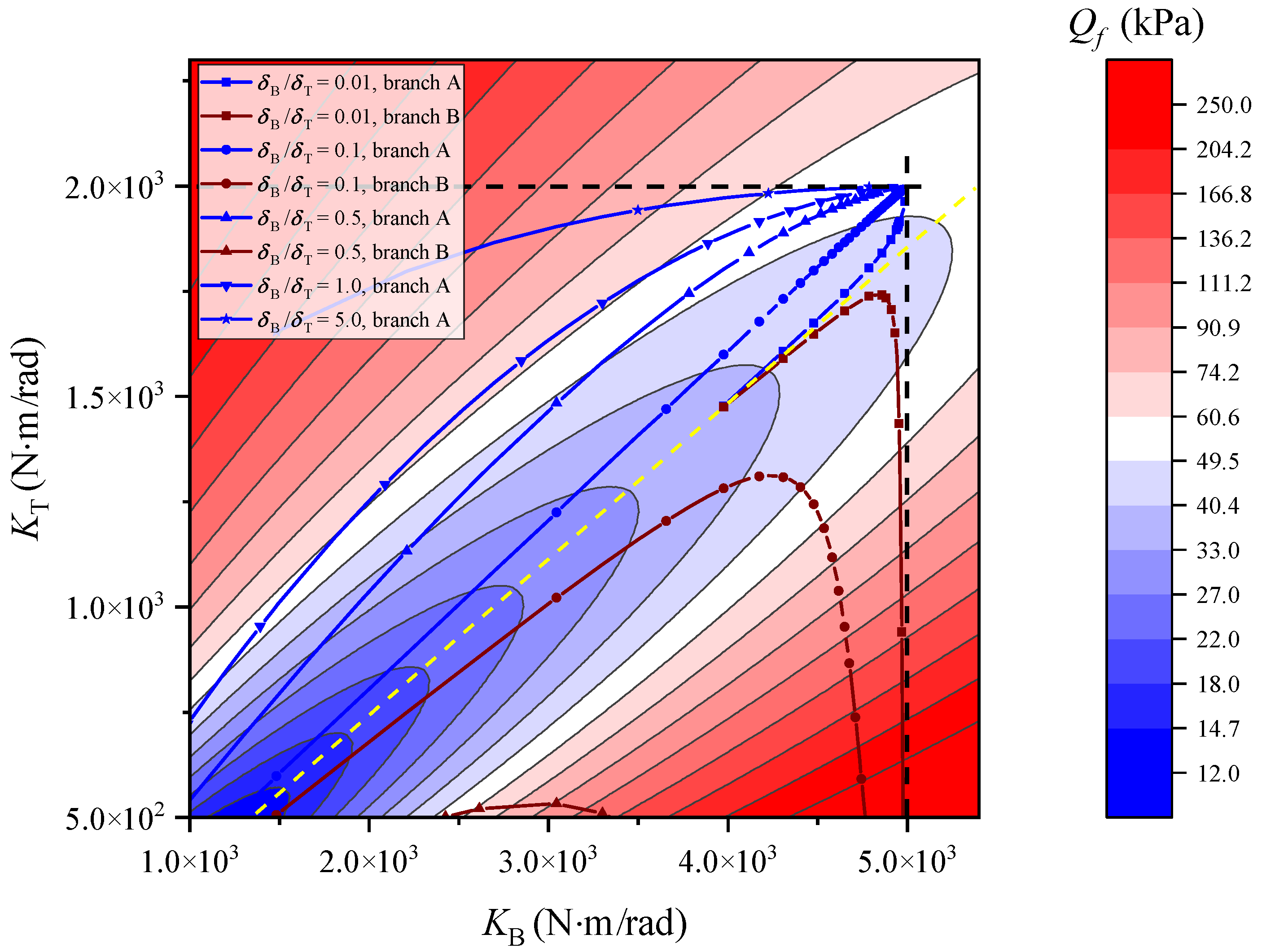
Here, we choose the former. According to Equation (14), is a monotonically increasing function of . For the subject of this study, is shown in Figure 8. Given different values that correspond to different values, the minimum point of R is roughly on the yellow dotted line. When is fixed, if is smaller than the value on the yellow dotted line, the right side of Equation (24) is a monotonically decreasing function of ; otherwise, the right side of Equation (24) first decreases and then increases with increasing . For the latter case, the LCO amplitude corresponding to the minimum R is recorded as here.
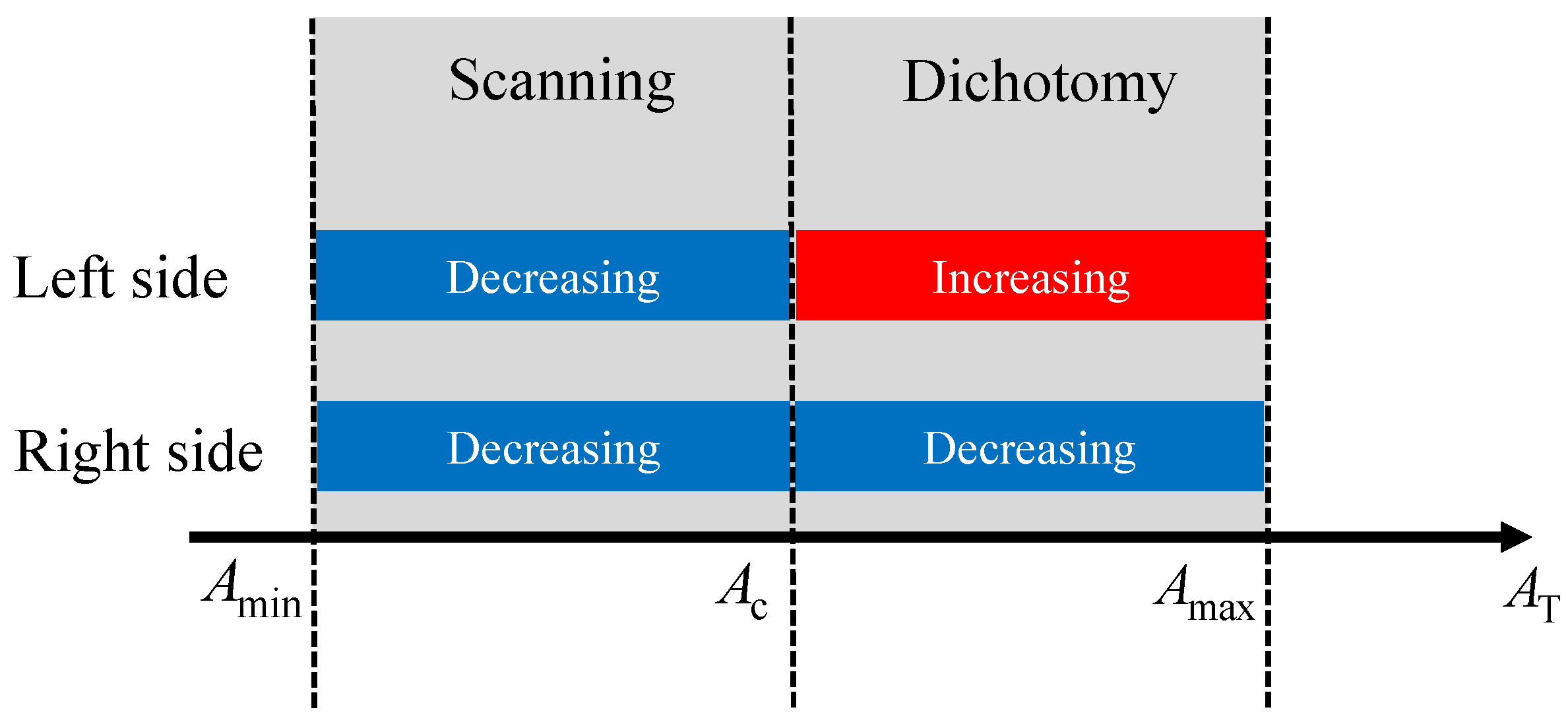
In contrast to previous studies, the ranges of the bending and torsional stiffnesses of the all-movable fin considered in this paper are very large so that its nonlinear aeroelastic characteristics can be comprehensively studied. The torsional stiffness may be relatively low, but no static divergence occurs. In this case, because the function on the right side of Equation (24) may not be monotonous, the previous iterative methods may cause a loss of solutions, and the iteration may not even converge. A more general method is to scan the entire solution interval to find the solutions of Equation (24). However, in the discrete scanning method proposed in this paper, a critical point is used to divide the solution interval into two parts: , where and are the specified minimum and maximum LCO amplitudes in the torsional DOF, respectively. As shown in Figure 9, when , the dichotomy method can be directly used because the left and right sides of the equation have different monotonicity. When , the scanning method is used. Compared with scanning the whole solution interval, this discrete scanning method improves the calculation efficiency while avoiding the loss of solutions.
Equation (24) can be expressed as:
where the nondimensional LCO amplitudes and can be considered as two variables, and the freeplay size ratio is a parameter. Therefore, in this paper is set to , and the freeplay size ratio is changed by using different values. The variation of the nondimensional LCO amplitudes with the dynamic pressure is obtained with different freeplay size ratios. It should be noted that although here is a definite value, no matter how it changes, as long as remains unchanged, the solution of the nondimensional LCO amplitudes and corresponding to the equation will not change; the only thing that changes is the corresponding LCO amplitudes and . Therefore, the nonlinear flutter characteristics of the system under different freeplay sizes and can be obtained by establishing the variation of the nondimensional LCO amplitudes of the system under different freeplay size ratios .
Here, is set to to avoid static aeroelastic divergence, and is set to 1000. The calculation error of in the dichotomy method is required to be less than . The scanning interval of is . When the scanning method is used, the computational domain is divided into n intervals: (). Then, we successively calculate the values . If , then we use the dichotomy method to find the solution of while .
3.2.2. Case 1: ,
In Case 1, a system with only a bending freeplay nonlinearity will exhibit LCO-ii characteristics; with only a torsion freeplay nonlinearity, it will exhibit LCO-i characteristics. Figure 10 shows the LCO solutions obtained by the discrete scanning method at different freeplay size ratios and the corresponding time-domain bifurcation diagrams. The dynamic pressure range for the time-domain analysis was from 15 kPa to the divergence dynamic pressure. Here, different LCO branches are defined according to the solving interval and the continuity of the LCO solutions with the parameters.
From the frequency-domain calculation results, we can find that there are two main LCO branches for each . Combined with the time-domain results, it can be found that when the freeplay size ratio is small, stable LCO motions appear below the linear flutter dynamic pressure. In addition, irregular motions with limited amplitude are observed in a certain region of dynamic pressure. With the increase of the freeplay size ratio, the dynamic pressure region of the LCO motions decreases, and the region of the irregular motions increases, but the amplitude tends to decrease. When the freeplay size ratio increases to , the nondimensional amplitude of the vibration is very small and almost entirely located near the freeplay boundary.
After the LCO solutions are obtained, the equivalent stiffness corresponding to the nondimensional LCO amplitude in the bending and torsional DOFs can be calculated. Therefore, each set of LCO nondimensional amplitudes will correspond to a point in Figure 6. Finally, complete LCO solutions at different can be drawn in the form of Figure 11. The yellow dotted line in Figure 11 is the same as in Figure 8. For each given , it divides the solution domain into upper and lower parts, which correspond to the solution intervals and . Finally, the results of branches A and B located on either side of the yellow line are obtained. The LCO solutions of a system with a single torsion or bending freeplay nonlinearity can be seen in the Figure 5 map to the right and the upper dotted lines in Figure 11, respectively.
When decreases, branch A gradually approaches the upper dotted line, and the LCO characteristics of a system with multiple freeplay nonlinearities are more similar to a system with only a torsion freeplay nonlinearity, that is, LCO-i. Similarly, when increases, the LCO characteristics tend to LCO-ii. Comparing the frequency-domain results at in Figure 5a and Figure 10, it can be inferred that when decreases to 0, the LCO of branch A finally will become the stable LCO branch in Figure 5a, while branch B becomes the unstable LCO branch. As increases to infinity, the LCO solutions in the bending DOF of branch A will finally become the unstable LCO branch in Figure 5b, while the LCO amplitude of branch B will be reduced to become negligible.
In summary, when the difference between the two freeplay sizes is large, the nonlinear aeroelastic characteristics of the system are mainly determined by the freeplay with the larger value. In addition, expressing the LCO solutions in the form of Figure 11 allows more concise and clear observation of the variation rule of the LCO characteristics of the system with the freeplay size ratio. This also contains the variation of the nondimensional LCO amplitude with dynamic pressure.
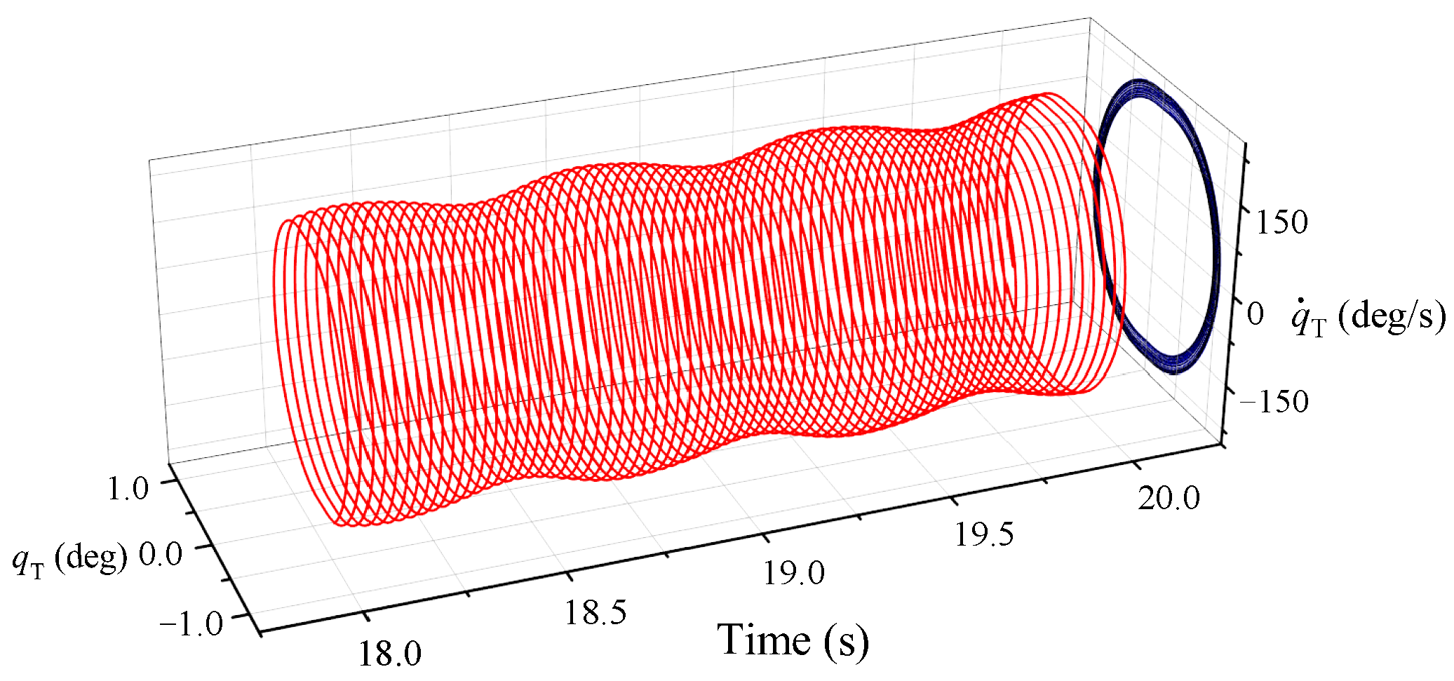
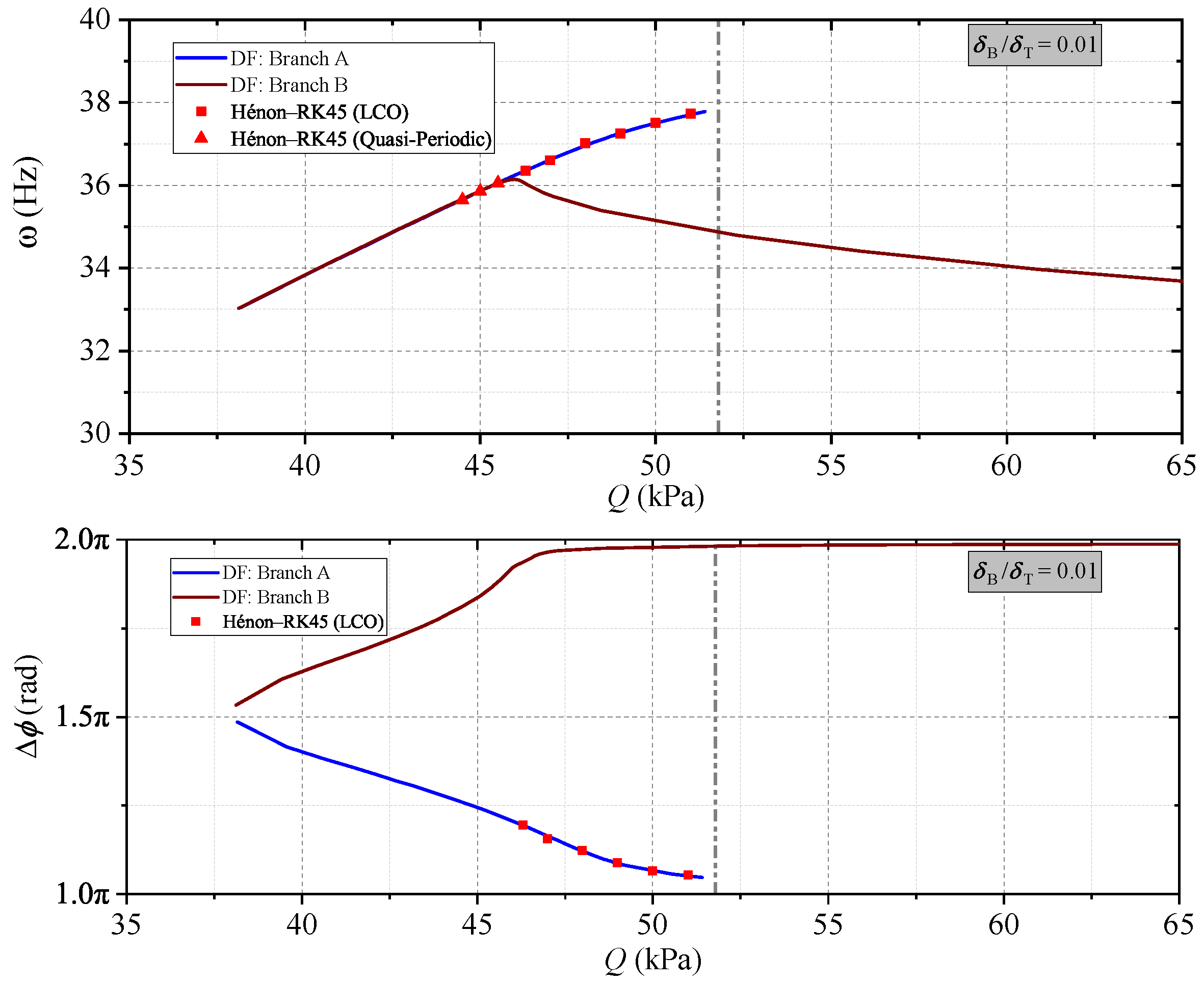
Further, we construct the Poincaré section by plotting against at time instances when and . For the Poincaré sections to be meaningful, the total simulation time was set to 200 s at each dynamic pressure state, and the last 100 s of data was selected for analysis. In Figure 12, dynamic pressures between kPa and kPa were chosen for the analysis at . Because the system response decays, the response trajectories do not intersect with the Poincaré section when the dynamic pressure is less than kPa. A closed curve appears suddenly at kPa, and at about kPa, this becomes a single point. Figure 13 shows a plot of the response trajectory of the system in the – phase plane at kPa. The response trajectory of the system is always within a torus. It can be clearly seen that a Hopf bifurcation occurs before kPa. The system response changes from decaying motions to quasi-periodic motions somewhere between and kPa, and it transforms into LCO motions at about kPa. From the frequency-domain LCO solutions in Figure 10, we can find two LCO branches that grow from a point around 38 kPa, which have a similar amplitude. Until approximately 46 kPa, the difference in the torsional LCO amplitude increases sharply due to the turning point of branch B. It can also be seen in Figure 11 that the two LCO branches start from one point and then gradually move away from each other when . Therefore, the appearances of such quasi-periodic motions are probably caused by the interaction between the two LCO branches, which should have similar amplitudes and irrational frequency ratios [42]. Once the two LCO branches move far away from each other, these quasi-periodic motions will be destroyed, and the response trajectories will be attracted by one of the LCO branches.
Figure 14 shows plots of the variations of the LCO frequency and the phase difference with dynamic pressure. The frequency of the quasi-periodic motion refers to the frequency of the component with the highest proportion. The frequency-domain calculation results show that the frequencies of the two LCO branches are relatively close until the turning point of the torsional LCO frequency at about kPa; however, the phase differences between the responses in the bending and torsional DOFs of the two branches have completely opposing trends. After the system enters the LCO at kPa, the frequency and phase of the time-domain LCO response are consistent with the LCO solutions of branch A. Figure 15 shows the spectral-analysis results of the time-domain response in the yellow area. Not surprisingly, we find that the LCO response at 47 kPa mainly contains the components of one frequency and its multiples, while the quasi-periodic motion at 45 kPa contains some irreducible frequencies. The frequency of the component with the highest proportion is consistent with the frequencies of the two LCO branches (Figure 14). However, some other frequency components cannot be obtained by the method in this paper; these may be generated by the coupling effects of LCO branches with similar amplitudes and frequencies but different phase differences. Another interesting phenomenon is that when the two LCO branches are very close, this quasi-periodic motion disappears, such as when the dynamic pressure is less than 44 kPa at or less than 28 kPa at .
To further study the transformation process of this quasi-periodic motion to the LCO, the time-domain response of systems with different dynamic pressures and initial conditions at was calculated, and the results are shown in Figure 16. When the default initial conditions are given, a quasi-periodic motion occurs at and kPa. If a harmonic initial condition corresponding to branch A is given, the response trajectory is immediately attracted to the LCO at kPa. However, at kPa, even given similar harmonic initial conditions, the amplitude of the system fluctuates increasingly as time goes on, and it eventually enters quasi-periodic motion. This phenomenon shows that with increasing dynamic pressure, the torsional LCO amplitude difference between the two branches expands, and this leads to the weakening of the coupling effect between the LCO branches. At kPa, when a harmonic initial condition corresponding to branch B is given, the system response decays. However, if the amplitude of the initial condition becomes times its original value, the system will eventually enter a stable LCO. This comparison indicates that the LCO of branch B is unstable at this dynamic pressure, and with sufficient initial amplitude, the system will be attracted to the stable LCO of branch A. In addition, we can find that the system at kPa with larger initial conditions has strong amplitude fluctuations at the beginning, but as time goes on, the fluctuations become progressively smaller, which is the complete opposite of the phenomenon at kPa. The above interesting phenomena reflect the weakening of the coupling effect of the two LCO branches and the expansion of the attraction domain of the stable LCO during the transformation process of the system from quasi-periodic motion to the LCO.
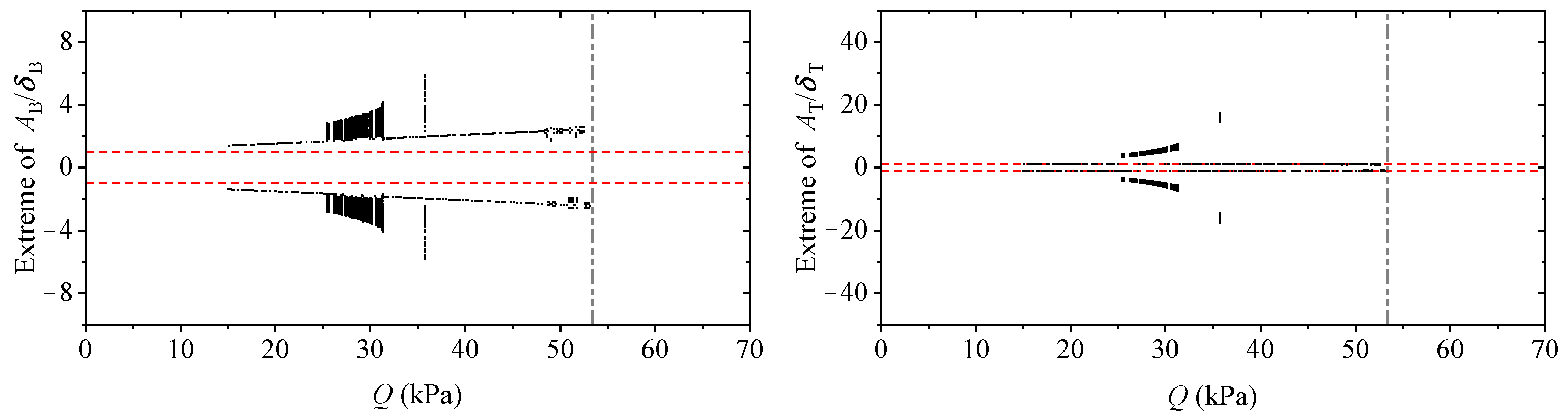
Figure 17 shows variations of the Poincaré section with dynamic pressure at and . Figure 18 shows the variation of the largest Lyapunov exponent with time [43,44], and it finally converges to a positive value with increasing time step N, indicating that the response of the system is a chaotic motion. Combined with Figure 12, it can be clearly seen that with increasing , the torus is gradually broken, and the system response gradually transitions from LCO and quasi-periodic motion to chaotic motion.
3.2.3. Case 2: ,
For the LCO characteristics of a system with a single freeplay nonlinearity, cases 2 and 1 are completely opposite. A system with only a bending freeplay nonlinearity will exhibit LCO-i characteristics, while one with only a torsion freeplay nonlinearity will exhibit LCO-ii characteristics. Figure 19 plots the LCO solutions obtained by the discrete scanning method and the corresponding time-domain bifurcation diagrams at different freeplay size ratios . Figure 20 plots the distribution of LCO solutions.
According to the solving interval and the continuity of the LCO solutions with the parameters, three LCO branches are defined here. In Figure 20, when , LCO branches A and B are located on either side of the yellow dotted line (two solution intervals) and converge at the top right. In contrast, branch C is relatively independent. With the decrease of , Branch C moves toward the right dotted line, and branches A and B move toward the yellow dotted line. The intersection point of branches A and B moves down and left, which means the right boundary of the dynamic pressure region of LCO branches A and B in Figure 19 is shifted to the left. If decreases to 0, LCO branches A and B would disappear and the system would exhibit LCO-ii characteristics similar to Figure 5b, as determined by the torsion freeplay. From the frequency-domain LCO solutions in Figure 19, there is no matching LCO solution in a certain dynamic pressure region when . The corresponding time-marching results show that the system response decays in this dynamic pressure region. Branch C is in the right of the region. This dynamic pressure region keeps shrinking with increasing , and it disappears completely at . Through further computational analysis, it was found that branches B and C meet and undergo recombination when is approximately . The relevant results are presented in Figure 20.
Later, with the increase of , branch B moves downward and eventually disappears in Figure 20, while branches A and C move toward the upper dotted line. The system exhibits LCO-i characteristics similar to Figure 5a, determined by the bending freeplay. Comparing the trend of at in Figure 20 with the trend of LCO-i in Figure 5a, it can be seen that branch A corresponds to the unstable LCO, and branch C corresponds to the stable LCO. The corresponding time-domain bifurcation diagram in Figure 20 also agrees well with the calculation results of branch C.
Next, we specifically look at the time-domain bifurcations of the system under different freeplay size ratios in Figure 19. At , the system response decays and eventually reaches a static equilibrium position when the dynamic pressure is lower than the linear flutter boundary. Due to the existence of the unstable LCO branch C, when the dynamic pressure is slightly higher than the linear flutter dynamic pressure, the system response does not diverge. This is because the initial conditions at this time are not of great enough amplitude to excite the system into a divergent state. The time-response results given in Figure 21 further verify the calculation results of the LCO branch C. However, the other two LCO branches A and B in the frequency-domain calculation results are not reflected in the corresponding time-domain bifurcation diagrams.
Considering that the current initial conditions might not excite the system to enter the LCO, we increased the amplitude of the initial conditions. The corresponding time-domain bifurcation diagrams are shown in Figure 22. When the initial conditions increase from 10 times the freeplay size to 100 times, quasi-periodic or chaotic motions appear between dynamic pressures of and kPa. However, the existence of such vibrations with a non-zero amplitude is uncertain because the system enters a decaying motion under some dynamic pressures between and kPa. In addition, a quasi-periodic motion occurs alone at kPa. In general, the existence of LCO branches A and B theoretically causes the system to exhibit more quasi-periodic or chaotic motions, but such vibrations are uncertain and have great dependencies on the initial conditions.
For the case of , the system mainly exhibits quasi-periodic or chaotic motions when the dynamic pressure is less than about 38 kPa. The nondimensional vibration amplitude also becomes larger as the dynamic pressure increases. As increases, the nondimensional vibration amplitude becomes smaller, but it changes more dramatically at around 38 kPa. Finally, the jumping phenomenon of the LCO appears at . When the dynamic pressure is higher than about 38 kPa but below the linear flutter boundary, the system exhibits LCO motions except for within the dynamic pressure region in which the response decays at .
Considering that , the nondimensional LCO amplitude increases with increasing dynamic pressure in the bending DOF, but it first decreases and then increases in the torsional DOF. There is a maximum value of the nondimensional LCO amplitude in the torsional DOF at around kPa; this should be carefully considered because structural damage can occur here.
4. Conclusions
This paper focused on the nonlinear aeroelastic characteristics of a small aspect ratio supersonic all-movable fin with single or multiple freeplay nonlinearities. The conclusions that can be drawn from the numerical results can be summarized as follows.
- (1)
- The DF method has shown good applicability to the analysis and solution of the LCO characteristics of the system with single or multiple freeplay nonlinearities. In this paper, a discrete scanning method based on the DF method was established to solve the problem of amplitude alignment, and this can avoid missing solutions and give consideration to efficiency.
- (2)
- Systems with a single freeplay nonlinearity exhibit two different types of LCO. A system with LCO-i characteristics has stable LCO motions below the linear flutter boundary, while a system with LCO-ii characteristics only has unstable LCO motions above the linear flutter boundary, and the divergence boundary is not lower than the linear flutter boundary. From a flutter suppression perspective, LCO-ii is more beneficial.
- (3)
- Systems with bending and torsion freeplay nonlinearities exhibit complex dynamical behaviors, such as LCO and quasi-periodic and chaotic motions. The initial conditions have a great influence on the system response. The introduction of harmonic initial conditions will effectively improve the efficiency of using time-domain integration to verify frequency-domain LCO solutions, especially for those with a small attraction domain.
- (4)
- The support stiffness at the root of the fin and freeplay size ratio have impressive effects on the LCO characteristics. The ratio of bending stiffness to torsional stiffness determines the LCO characteristics of a fin with a single freeplay nonlinearity. For a fin with multiple freeplay nonlinearities, when the difference between the two freeplay sizes is large, its nonlinear aeroelastic characteristics are mainly determined by the freeplay with the larger value.
The small aspect ratio fin in this paper is treated as a rigid fin because its elastic modes have higher frequencies and have little influence on the flutter characteristics of the fin. However, for the flexible fin with a high aspect ratio, the elastic modes cannot be ignored. Further research is needed to investigate the influence of the elastic modes. In addition, damping is not involved in this paper, and the suppression effect of damping on the vibrations of the fin with multiple freeplay nonlinearities needs further study.
Author Contributions
Conceptualization, Z.W. and L.B.; methodology, Z.W. and L.B.; software, L.B.; validation, Z.W. and L.B.; formal analysis, L.B.; writing—original draft preparation, L.B.; writing—review and editing, Z.W.; supervision, C.Y.; project administration, C.Y. All authors have read and agreed to the published version of the manuscript.
Funding
This research received no external funding.
Institutional Review Board Statement
Not applicable.
Informed Consent Statement
Not applicable.
Data Availability Statement
Not applicable.
Conflicts of Interest
The authors declare no conflict of interest.
Abbreviations
| LCO | limit-cycle oscillation |
| DOF | degree-of-freedom |
| DF | describing function |
| RK45 | fourth–-fifth-order Runge–-Kutta |
| 3D | three-dimensional |
References
- Panchal, J.; Benaroya, H. Review of control surface freeplay. Prog. Aeronaut. Sci. 2021, 127, 100729. [Google Scholar] [CrossRef]
- Dowell, E.H.; Edwards, J.; Strganac, T. Nonlinear aeroelasticity. J. Aircr. 2003, 40, 857–874. [Google Scholar] [CrossRef]
- Danowsky, B.; Thompson, P.M.; Kukreja, S. Nonlinear analysis of aeroservoelastic models with free play using describing functions. J. Aircr. 2013, 50, 329–336. [Google Scholar] [CrossRef]
- Woolston, D.S.; Runyan, H.L.; Andrews, R.E. An Investigation of Effects of Certain Types of Structural NonHnearities on Wing and Control Surface Flutter. J. Aeronaut. Sci. 1957, 24, 57–63. [Google Scholar] [CrossRef]
- Shen, S.F. An Approximate Analysis of Nonlinear Flutter Problems. J. Aerosp. Sci. 1959, 26, 25–32. [Google Scholar] [CrossRef]
- Yang, Z.; Zhao, L. Analysis of limit cycle flutter of an airfoil in incompressible flow. J. Sound Vibr. 1988, 123, 1–13. [Google Scholar] [CrossRef]
- Lee, B.H.K.; Tron, A. Effects of structural nonlinearities on flutter characteristics of the CF-18 aircraft. J. Aircr. 1989, 26, 781–786. [Google Scholar] [CrossRef]
- Lee, I.; Kim, S.H. Aeroelastic analysis of a flexible control surface with structural nonlinearity. J. Aircr. 1995, 32, 868–874. [Google Scholar] [CrossRef]
- Tang, D.; Dowell, E.H.; Virgin, L. Limit cycle behavior of an airfoil with a control surface. J. Fluids Struct. 1998, 12, 839–858. [Google Scholar] [CrossRef]
- Padmanabhan, M.A.; Dowell, E.H. Gust Response Computations with Control Surface Freeplay Using Random Input Describing Functions. AIAA J. 2020, 58, 2899–2908. [Google Scholar] [CrossRef]
- Wayhs-Lopes, L.D.; Dowell, E.H.; Bueno, D.D. Influence of friction and asymmetric freeplay on the limit cycle oscillation in aeroelastic system: An extended Hénon’s technique to temporal integration. J. Fluids Struct. 2020, 96, 103054. [Google Scholar] [CrossRef]
- Iannelli, A.; Lowenberg, M.; Marcos, A. On the effect of model uncertainty on the Hopf bifurcation of aeroelastic systems. Nonlinear Dyn. 2021, 103, 1453–1473. [Google Scholar] [CrossRef]
- Wang, X.; Wu, Z.; Yang, C. Integration of Freeplay-Induced Limit Cycles Based On a State Space Iterating Scheme. Appl. Sci. 2021, 11, 741. [Google Scholar] [CrossRef]
- Hénon, M. On the numerical computation of Poincaré maps. Physica D 1982, 5, 412–414. [Google Scholar] [CrossRef]
- Conner, M.D.; Virgin, L.N.; Dowell, E.H. Accurate numerical integration of state-space models for aeroelastic systems with free play. AIAA J. 1996, 34, 2202–2205. [Google Scholar] [CrossRef]
- Dai, H.; Yue, X.; Yuan, J.; Xie, D.; Atluri, S. A comparison of classical Runge-Kutta and Henon’s methods for capturing chaos and chaotic transients in an aeroelastic system with freeplay nonlinearity. Nonlinear Dyn. 2015, 81, 169–188. [Google Scholar] [CrossRef]
- Lee, B.; Price, S.; Wong, Y. Nonlinear aeroelastic analysis of airfoils: Bifurcation and chaos. Prog. Aeronaut. Sci. 1999, 35, 205–334. [Google Scholar] [CrossRef]
- Bueno, D.D.; Wayhs-Lopes, L.D.; Dowell, E.H. Control-Surface Structural Nonlinearities in Aeroelasticity: A State of the Art Review. AIAA J. 2022, 60, 3364–3376. [Google Scholar] [CrossRef]
- Padmanabhan, M.A.; Pasiliao, C.L.; Dowell, E.H. Simulation of Aeroelastic Limit-Cycle Oscillations of Aircraft Wings with Stores. AIAA J. 2014, 52, 2291–2299. [Google Scholar] [CrossRef]
- Padmanabhan, M.A.; Dowell, E.H. Calculation of Aeroelastic Limit Cycles due to Localized Nonlinearity and Static Preload. AIAA J. 2017, 55, 2762–2772. [Google Scholar] [CrossRef]
- Padmanabhan, M.A.; Dowell, E.H.; Pasiliao, C.L. Computational Study of Aeroelastic Limit Cycles due to Localized Structural Nonlinearities. J. Aircr. 2018, 55, 1531–1541. [Google Scholar] [CrossRef]
- Huang, R.; Hu, H.; Zhao, Y. Nonlinear aeroservoelastic analysis of a controlled multiple-actuated-wing model with free-play. J. Fluids Struct. 2013, 42, 245–269. [Google Scholar] [CrossRef]
- Huang, R.; Zhou, X. Parameterized Fictitious Mode of Morphing Wing with Bilinear Hinge Stiffness. AIAA J. 2021, 59, 2641–2656. [Google Scholar] [CrossRef]
- Tang, D.; Dowell, E.H. Aeroelastic Response Induced by Free Play, Part 1: Theory. AIAA J. 2011, 49, 2532–2542. [Google Scholar] [CrossRef]
- Tang, D.; Dowell, E.H. Aeroelastic Response Induced by Free Play, Part 2: Theoretical/Experimental Correlation Analysis. AIAA J. 2011, 49, 2543–2554. [Google Scholar] [CrossRef]
- Yang, N.; Wang, N.; Zhang, X.; Liu, W. Nonlinear flutter wind tunnel test and numerical analysis of folding fins with freeplay nonlinearities. Chin. J. Aeronaut. 2016, 29, 144–159. [Google Scholar] [CrossRef] [Green Version]
- He, H.; Tang, H.; Yu, K.; Li, J.; Yang, N.; Zhang, X. Nonlinear aeroelastic analysis of the folding fin with freeplay under thermal environment. Chin. J. Aeronaut. 2020, 33, 2357–2371. [Google Scholar] [CrossRef]
- Karpel, M.; Raveh, D. Fictitious mass element in structural dynamics. AIAA J. 1996, 34, 607–613. [Google Scholar] [CrossRef]
- Firouz-Abadi, R.; Alavi, S.; Salarieh, H. Analysis of non-linear aeroelastic response of a supersonic thick fin with plunging, pinching and flapping free-plays. J. Fluids Struct. 2013, 40, 163–184. [Google Scholar] [CrossRef]
- Laurenson, R.M.; Trn, R.M. Flutter Analysis of Missile Control Surfaces Containing Structural Nonlinearities. AIAA J. 1980, 18, 1245–1251. [Google Scholar] [CrossRef]
- Breitbach, E.J. Flutter Analysis of an Airplane with Multiple Structural Nonlinearities in the Control System; Technical Report; NASA: Washington, DC, USA, 1980. [Google Scholar]
- Lee, C.L. An iterative procedure for nonlinear flutter analysis. AIAA J. 1986, 24, 833–840. [Google Scholar] [CrossRef]
- Seo, Y.J.; Lee, S.J.; Bae, J.S.; Lee, I. Effects of multiple structural nonlinearities on limit cycle oscillation of missile control fin. J. Fluids Struct. 2011, 27, 623–635. [Google Scholar] [CrossRef]
- Gladwell, G.M.L. Branch mode analysis of vibrating systems. J. Sound Vib. 1964, 1, 41–59. [Google Scholar] [CrossRef]
- Tian, W.; Yang, Z.; Zhao, T. Nonlinear aeroelastic characteristics of an all-movable fin with freeplay and aerodynamic nonlinearities in hypersonic flow. Int. J. Non-Linear Mech. 2019, 116, 123–139. [Google Scholar] [CrossRef]
- Bai, L.; Wu, Z.; Yang, C. Nonlinear flutter modes and flutter suppression of an all-movable fin with freeplay. J. Beijing Univ. Aeronaut. Astronaut. 2022. (In Chinese) [Google Scholar] [CrossRef]
- Hayes, W.D. On hypersonic similitude. Q. Appl. Math. 1947, 5, 105–106. [Google Scholar] [CrossRef] [Green Version]
- Lighthill, M.J. Oscillating Airfoils at High Mach Number. J. Aeronaut. Sci. 1953, 20, 402–406. [Google Scholar] [CrossRef]
- Liu, D.D.; Yao, Z.X.; Sarhaddi, D.; Chavez, F. From Piston Theory to a Unified Hypersonic-Supersonic Lifting Surface Method. J. Aircr. 1997, 34, 304–312. [Google Scholar] [CrossRef]
- Van Dyke, M.D. A Study of Second-Order Supersonic Flow Theory; Technical Report; NASA: Washington, DC, USA, 1952. [Google Scholar]
- Strang, G. Linear Algebra and Its Applications; Thomson, Brooks/Cole: Belmont, CA, USA, 2006. [Google Scholar]
- Dimitriadis, G. Introduction to Nonlinear Aeroelasticity; John Wiley & Sons: Hoboken, NJ, USA, 2017. [Google Scholar]
- Wolf, A.; Swift, J.B.; Swinney, H.L.; Vastano, J.A. Determining Lyapunov exponents from a time series. Phys. D 1985, 16, 285–317. [Google Scholar] [CrossRef]
- Sprott, J.C. Chaos and Time-Series Analysis; Oxford University Press: Oxford, UK, 2003. [Google Scholar]
Figure 1.
Simplified model of the all-movable fin examined in this paper.

Figure 2.
Geometrical schematic of the all-movable fin. All dimensions are in millimeters.

Figure 3.
Mode shapes of the all-movable fin.

Figure 4.
Linear flutter dynamic pressure with the variation of torsional or bending stiffness. (I: monotonically increasing; II: monotonically decreasing).
Figure 4.
Linear flutter dynamic pressure with the variation of torsional or bending stiffness. (I: monotonically increasing; II: monotonically decreasing).

Figure 5.
Nonlinear aeroelastic characteristics of an all-movable fin with torsion or bending freeplay (, ).
Figure 5.
Nonlinear aeroelastic characteristics of an all-movable fin with torsion or bending freeplay (, ).

Figure 6.
Linear flutter dynamic pressure with the variation of bending and torsional stiffnesses. The LCO characteristics of the all-movable fin with bending or torsion freeplay nonlinearity in linear states (i) and (ii) are shown, respectively.
Figure 6.
Linear flutter dynamic pressure with the variation of bending and torsional stiffnesses. The LCO characteristics of the all-movable fin with bending or torsion freeplay nonlinearity in linear states (i) and (ii) are shown, respectively.

Figure 7.
Observation of the unstable LCO and the application of the harmonic initial condition in time-domain integration (, , ).
Figure 7.
Observation of the unstable LCO and the application of the harmonic initial condition in time-domain integration (, , ).

Figure 8.
Changes in flutter modal amplitude ratio R with and .

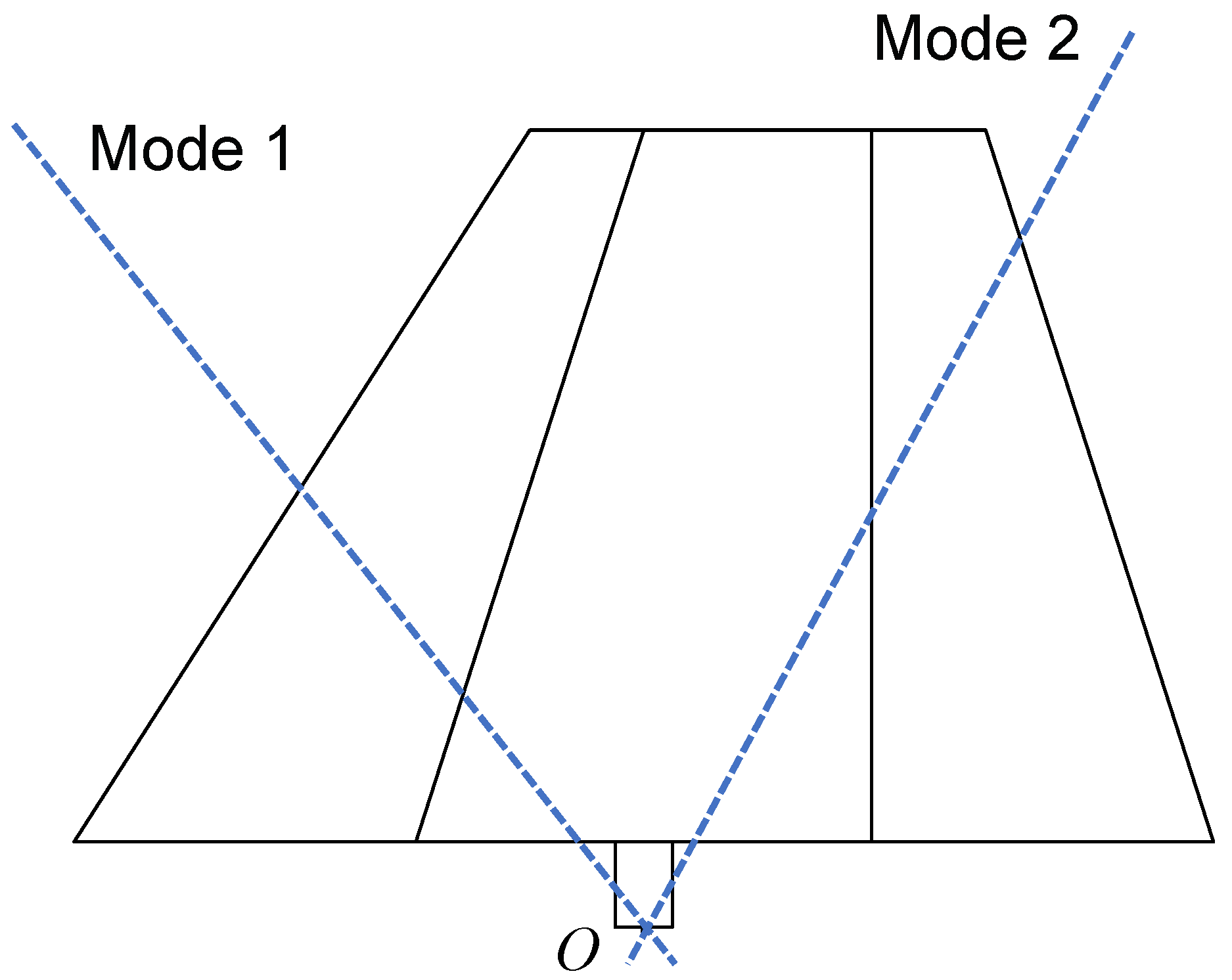
Figure 9.
The process of solving Equation (24) by discrete scanning method.
Figure 9.
The process of solving Equation (24) by discrete scanning method.

Figure 10.
Frequency-domain LCO solutions and corresponding time-domain bifurcation diagrams in bending and torsional DOFs ( is , , , , and from top to bottom).
Figure 10.
Frequency-domain LCO solutions and corresponding time-domain bifurcation diagrams in bending and torsional DOFs ( is , , , , and from top to bottom).

Figure 11.
LCO solutions on linear flutter dynamic pressure nephogram (, ).

Figure 12.
Poincaré section variation with dynamic pressure at . The sampling interval is kPa.

Figure 13.
Response trajectory of the system in the – phase plane at kPa and .

Figure 14.
LCO frequency and phase-difference variations with dynamic pressure at .

Figure 15.
Time responses and spectra for 45 and 47 kPa and .

Figure 16.
Time responses of systems at different dynamic pressures and initial conditions. ( kPa: harmonic initial conditions of branch A (right); kPa: harmonic initial conditions of branch A (right); kPa: harmonic initial conditions of branch B (left), times the left initial conditions (right). . The phase parameter of the harmonic initial condition is set to .)

Figure 17.
Variation of Poincaré sections with dynamic pressure at different values. The sampling interval is kPa.
Figure 17.
Variation of Poincaré sections with dynamic pressure at different values. The sampling interval is kPa.

Figure 18.
Variation of the largest Lyapunov exponent with time at 45 kPa and .

Figure 19.
Frequency-domain LCO solutions and corresponding time-domain bifurcation diagrams in bending and torsional DOFs (, , and is , , , , and from top to bottom).
Figure 19.
Frequency-domain LCO solutions and corresponding time-domain bifurcation diagrams in bending and torsional DOFs (, , and is , , , , and from top to bottom).

Figure 20.
LCO solutions on linear flutter dynamic pressure nephogram (, ).

Figure 21.
Time-domain responses of the system with different initial conditions at . The phase parameter of the harmonic initial condition is set to ).
Figure 21.
Time-domain responses of the system with different initial conditions at . The phase parameter of the harmonic initial condition is set to ).

Figure 22.
Time-domain bifurcation diagrams of LCO responses when [, ] at .


Table 1.
Structure parameters of the all-movable fin.
| Parameter | Description | Value |
|---|---|---|
| m | Mass | |
| Mass moment of inertia | ||
| Mass moment of inertia | ||
| Mass moment of inertia | ||
| Bending spring stiffness | ||
| Torsional spring stiffness | ||
| Center-of-gravity position |
Table 2.
Linear flutter results of the all-movable fin.
| Parameter | Description | Value |
|---|---|---|
| Modal frequency of mode 1 | ||
| Modal frequency of mode 2 | ||
| Flutter velocity | ||
| Flutter dynamic pressure | ||
| Flutter frequency |
Disclaimer/Publisher’s Note: The statements, opinions and data contained in all publications are solely those of the individual author(s) and contributor(s) and not of MDPI and/or the editor(s). MDPI and/or the editor(s) disclaim responsibility for any injury to people or property resulting from any ideas, methods, instructions or products referred to in the content. |
© 2023 by the authors. Licensee MDPI, Basel, Switzerland. This article is an open access article distributed under the terms and conditions of the Creative Commons Attribution (CC BY) license (https://creativecommons.org/licenses/by/4.0/).
Share and Cite
MDPI and ACS Style
Bai, L.; Wu, Z.; Yang, C. Nonlinear Aeroelastic Characteristics of a Supersonic All-Movable Fin with Single or Multiple Freeplay Nonlinearities. Appl. Sci. 2023, 13, 1262. https://0-doi-org.brum.beds.ac.uk/10.3390/app13031262
AMA Style
Bai L, Wu Z, Yang C. Nonlinear Aeroelastic Characteristics of a Supersonic All-Movable Fin with Single or Multiple Freeplay Nonlinearities. Applied Sciences. 2023; 13(3):1262. https://0-doi-org.brum.beds.ac.uk/10.3390/app13031262
Chicago/Turabian StyleBai, Liuyue, Zhigang Wu, and Chao Yang. 2023. "Nonlinear Aeroelastic Characteristics of a Supersonic All-Movable Fin with Single or Multiple Freeplay Nonlinearities" Applied Sciences 13, no. 3: 1262. https://0-doi-org.brum.beds.ac.uk/10.3390/app13031262
Note that from the first issue of 2016, this journal uses article numbers instead of page numbers. See further details here.