Article

Cone Beam Computed Tomography Radiomics for Prostate Cancer: Favourable vs. Unfavourable Prognosis Prediction

1
Centro de Investigação do Instituto Português de Oncologia do Porto (CI-IPOP), Grupo de Física Médica, Radiobiologia e Protecção Radiológica, 4200-072 Porto, Portugal
2
Faculdade de Engenharia da Universidade do Porto (FEUP), 4200-465 Porto, Portugal
3
Instituto Superior de Engenharia de Coimbra (ISEC), 3030-199 Coimbra, Portugal
4
Instituto de Ciências Biomédicas Abel Salazar (ICBAS), 4050-313 Porto, Portugal
*
Author to whom correspondence should be addressed.
Submission received: 30 November 2022 / Revised: 13 January 2023 / Accepted: 17 January 2023 / Published: 20 January 2023
(This article belongs to the Special Issue Cutting Edge Advances in Image Information Processing)

Abstract

:
Silently asymptomatic at an early stage and often painless, requiring only active surveillance, Prostate Cancer (PCa) is traditionally diagnosed by a Digital Rectal Examination (DRE) and a Prostate Specific Antigen (PSA) blood test. A histological examination, searching for pattern irregularities on the prostate glandular tissue, is performed to quantify the aggressiveness of PCa. The assigned Gleason Score (GS), usually combined with Transrectal Ultrasound Guided Biopsy (TRUS), allows the stratification of patients according to their risk group. Intermediate-risk patients may have a favourable (GS = 3 + 4) or unfavourable (GS = 4 + 3) prognosis. This borderline is critical for defining treatments and possible outcomes, while External Beam Radiotherapy (EBRT) is a curative option for localised and locally advanced disease and as a palliative option for metastatic low-volume disease; active surveillance or watchful waiting can also be an option for patients with a favourable prognosis. With radiomics, quantifying phenotypic characteristics in medical imaging is now possible. In the EBRT workflow, there are several imaging modalities, such as Magnetic Ressonance Imaging (MRI), Computed Tomography (CT), Positron Emission Tomography (PET), Ultrasound and Cone Beam Computed Tomography (CBCT). Most radiomic PCa studies focused on MRI and addressed tumour staging, GS, PSA or Biochemical Recurrence (BCR). This study intends to use CBCT radiomics to distinguish between favourable and unfavourable cases, with the potential of evaluating an ongoing treatment. Seven of the most used feature selection methods, combined with 14 different classifiers, were evaluated in a total of 98 pipelines. From those, six stood out with Area Under the Receiver Operating Characteristic (AUROC) values ≥ 0.79. To the best of our knowledge, this is the first work to evaluate a PCa favourable vs. unfavourable prognosis model based on CBCT radiomics.

1. Introduction

In 1853, John Adams, a surgeon at the London Hospital, diagnosed a cirrhosis of the prostate gland as an orphan disease, the first described case of Prostate Cancer (PCa). In 2020, the disease was responsible for 7.3% of all cancer deaths in men and was the second most frequent malignancy [
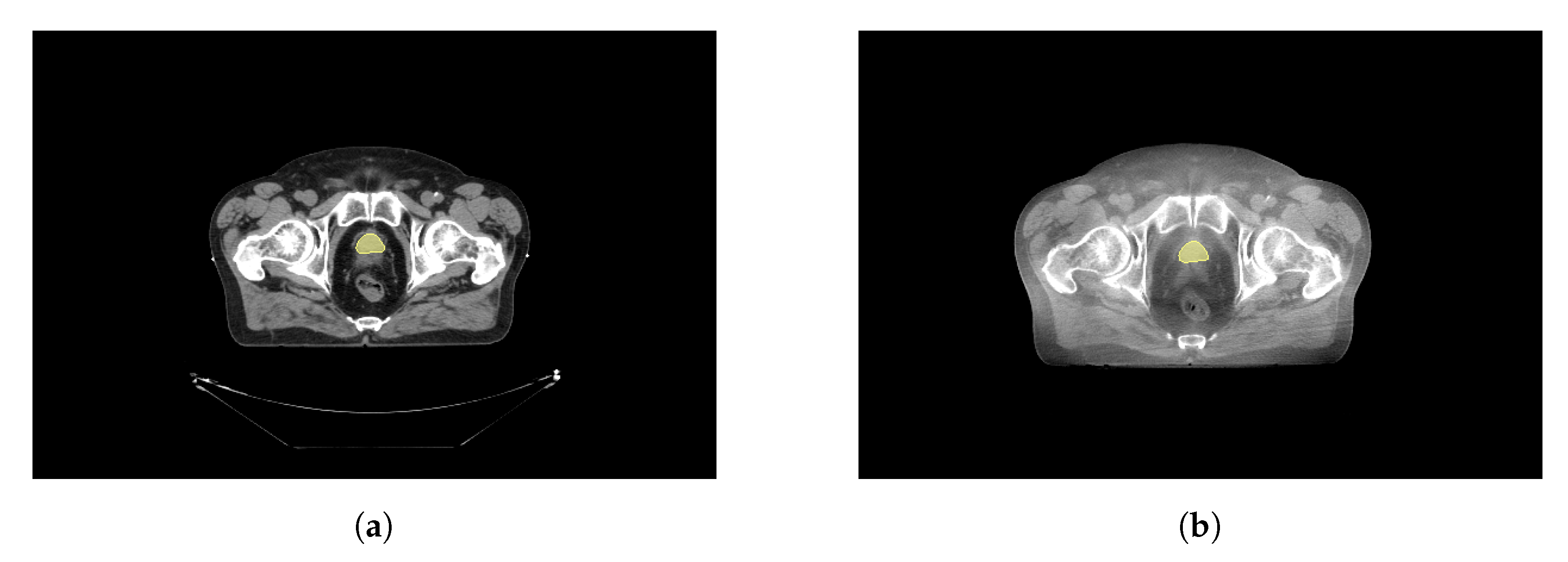
1]. The prostate gland is about the size of a walnut and located in the pelvis surrounding the prostatic urethra and below the bladder. Usually, PCa originates from the peripheral zone of the prostate, adjacent to the rectum [2]. Silently asymptomatic in an early stage, PCa is usually diagnosed by a Digital Rectal Examination (DRE) and a Prostate Specific Antigen (PSA) blood test.
The aggressiveness of PCa is quantified by the Gleason Grading System [3]. Based on the glandular architecture of cells, the pathologist assigns a grade of 1 if prostate cells are uniformly packed, up to a grade of 5 depending on pattern irregularity. The most predominant pattern and the second most prevalent are identified and graded accordingly, and finally summed to obtain the Gleason Score (GS), proportional to PCa aggressiveness [4]. In 2014, Epstein et al. [5] proposed a new Gleason grading system when several studies showed that a GS 7 = 4 + 3 had a worst prognosis than GS 7 = 3 + 4. A deeper stratification by Grade Group (GG) was then possible, including the most likely prognosis. The low/very low Risk Group (RG) is assigned to patients with a GS 6 . The intermediate RG includes patients classified with a GS of 7, with both favourable (3+4) and unfavourable (4+3) prognosis. Finally, the high/very high RG includes patients with a GS > 7 .
GS plays an important role in the determination of the type of treatment to follow. A low-grade cancer with a GS 6, together with a low PSA level and a small tumor may be an indication for active surveillance only. PCa evaluation takes into account the PSA levels, GS, TNM, patient history and physical examinations in order to provide a decision baseline for proper treatment and success prediction. Current guidelines suggest External Beam Radiotherapy (EBRT) as a curative option for localised and locally advanced disease and as a palliative option for metastatic low-volume disease [6]. The effectiveness of the treatment usually relies on the monitoring of PSA blood levels, the current reference biological test. Although a high value is associated with an increased risk of PCa, it is not PCa specific. High values of PSA are also associated with Benign Prostatic Hyperplasia (BPH), an enlarged prostate gland [7]. With the wide availability of PSA tests and the known long-term effects of definitive therapy, overdiagnosis and overtreatment have become a major issue. PCa treatments may cause sexual dysfunction, infertility, bowel and urinary problems [6], and so more conservative approaches such as active surveillance or watchful waiting have been adopted [8]. These are valid options, even for intermediate risk patients with a favourable prognosis (GS = 3 + 4).
During the EBRT workflow, many imaging modalities are available. The Computed Tomography (CT) provides the Hounsfield Unit (HU) values critical for dose estimations. For PCa, Magnetic Ressonance Imaging (MRI), providing superior soft-tissue resolution, is used for volume delineation. Positron Emission Tomography (PET) provides tumour cells’ metabolic insights and finally, the Cone Beam Computed Tomography (CBCT), acquired during EBRT sessions, is used for patient positioning and setup verifications. Quantitative analysis of medical images may have a similar prognosis power to phenotypes and gene protein signatures [9]. This is the hypothesis behind radiomics (the extraction of features from radiographic images using data-characterization algorithms). As an emerging field in medicine, radiomics provides the quantification of phenotypic characteristics in medical imaging [10]. Traditionally, image analysis and characterization of shape, texture or patterns is performed by highly trained human observers, but radiomics can provide quantitative image analysis without inter/intra observer variability.
Radiomic studies have recently triggered the interest of the research community, and for PCa are mainly focused on several predictive outcomes such as staging, grading, detection, Biochemical Recurrence (BCR) or aggressiveness. Furthermore, the most used imaging modality is MRI, which is usually performed in the initial stages and is critical for volume delineation. With the predictive and phenotypic power of radiomics, other imaging modalities besides MRI may provide valuable insights. Mendes et al. [11] evaluated CT based radiomics to predict PCa aggressiveness with promising results. In a novel attempt, Bosetti et al. [12] evaluated the use of CBCT radiomics to address tumour staging, GS, PSA, RG and BCR. Monitoring and classifying the outcome prognosis during treatment may help to avoid extra-invasive procedures or another MRI. This work intends to evaluate a model in borderline favourable vs. unfavourable (3+4 vs. 4+3) PCa cases, providing a tool that may trigger a more conservative approach, avoiding over-treatment and reducing the side effects of radiation exposure.
Following this introductory section is a summary of some of the work done in PCa radiomics using multiple imaging modalities. The idea is to gather information on the most-used feature selection and classification techniques. Section 3 describes the dataset and the methods used to build the evaluated pipelines. Section 4 presents the obtained results, highlighting the six best pipelines (from 98 evaluated). Finally, Section 5 presents the main conclusions drawn.

2. Related Work

Radiomics, the extraction of quantitative features from medical images using data characterization algorithms, has the potential to provide more relevant information, improve decision outcomes and avoid overdiagnosis and overtreatment. A full radiomic study follows a pipeline initially proposed by Lambin et al. [13] involving several steps, as exemplified in Figure 1.
Many imaging modalities are of great value in screening PCa and improving diagnosis and prognosis outcomes [14]. MRI provides superior soft-tissue contrast resolution when compared to other imaging modalities. It is the selected imaging modality by Prostate Imaging Reporting and Data System (PIRADS). Most radiomic studies are focused on MRI with the PCa clinical significance as a model endpoint [15,16,17,18,19,20,21]. The combination of T1 and T2 weighted sequences (multi-parametric Magnetic Ressonance Imaging (mpMRI)) allows us to overcome the poor correlation between MRI signal intensities and tissue properties. With this in mind, several authors evaluated the use of MRI for PCa patient stratification with promising results [16,17,18,19], although the introduction of clinical outcomes such as PSA or GS introduced some issues [20]. Abraham and Nair [22] topped the PROSTATEx-2 2017 challenge with a quadratic-weighted kappa score of 0.2772, developing a new feature selection method for PCa aggressiveness assessment. Algohary et al. [23] sought a model to evaluate Intensity Modulated Radiation Therapy (IMRT) PCa treatment responses using T2w and Apparent Diffusion Coefficient (ADC) maps in an attempt to personalize the PCa treatment evaluation framework.
PET provides insights into the pathological responses to some types of cancers with the addition of a radio-tracer and a viable tool for diagnosing, staging and grading. For radiomic PCa studies, researchers focused on evaluating lymph node involvement, metastasis, GS and extra-capsular extension [24]. Alongi et al. [25] evaluated tumour heterogeneity with 18F-Cho-PET/CT radiomics and introduced a novel feature selection method (a mixed descriptive-inferential sequential approach).
CT seems to be a poor candidate for radiomic studies since it lacks metabolic manifestation and soft-tissue contrast. However, the spatial distribution provided by the CT could be used as a virtual biopsy for patient risk stratification [26]. In a recent work, Mendes et al. [11] evaluated the use of CT based radiomics for PCa aggressiveness assessment. With a dataset of 44 PCa patients, Mendes et al. [11] extracted features using pyradiomics [10] and Local Image Features Extraction (LIFEx) [27]. Unable to find a radiomic signature for RG stratification, they used Principal Component Analysis (PCA) and evaluated several kernels to build a model with a Support Vector Machine (SVM). The best results were obtained with pyradiomics with a maximum Area Under the Receiver Operating Characteristic (AUROC) value of 0.88 for both low/very low and high/very high RG.
CBCT is used for patient positioning verification procedures before EBRT treatment and therefore is freely available. Bosetti et al. [12] were the first to study the use of CBCT radiomics to build models predicting tumour staging, GS, PSA levels, risk category and biochemical recurrence with promising results. In this work, we intend to evaluate the use of CBCT radiomics to distinguish between favourable and unfavourable PCa cases. An unevaluated scenario that may provide an EBRT treatment effectiveness monitoring tool is used.

3. Materials and Methods

This work is a retrospective piece of research that uses treatment plans available at Instituto Português de Oncologia do Porto Francisco Gentil (IPO-PORTO). All patients had an initial CT scan, required for dose estimation and volume delineations, and CBCT of the first EBRT treatment session, used for patient positioning setup verification. The full analysis was performed on an Intel(R) Core(TM) i7-6500U [email protected] 2.60 GHzz, with 16 Gb of RAM and an Nvidia GeForce 930M (2Gb DDR3).

3.1. Study Population

This study includes a subset of patients from a dataset containing CT and CBCT images from 70 patients. All studies ranged from 2019 to 2021 with curative intent, and patients were between 51 and 89 years old. CT images were acquired in a 16 slice CT scanner from General Electric, GE Optima 580 available at the IPO-PORTO for EBRT, acquired at 120 kVp, with 2.500 mm of slice thickness, automatic tube current modulation, a pixel spacing of 0.976 × 0.976 and 16 bits of pixel depth. For the same patients CBCT images were acquired from the on-board imaging devices installed in NOVALIS, TRUEBEAM and TRILOGY Medical Linear Accelerators (LINACs) from Varian. Acquisition settings depend on the LINAC and are shown on Table 1.
Clinical information such as the GS, PSA levels, TNM and also staging, when available, was collected. The dataset was grouped following a 3-fold GS risk group stratification as proposed by Epstein et al. [5]. The selected subset included only patients classified as intermediate risk. The idea was to develop a tool capable of distinguishing favourable and unfavourable clinical outcomes and also a baseline for a EBRT effectiveness assessment. Following these criteria, this study included 22 patients with a favourable outcome (GS = 3 + 4 and GG = 2) and 24 patients with an unfavourable outcome (GS = 4 + 3 and GG = 3), as shown in Table 2 (in bold font).

3.2. Image Registration

In EBRT, in the treatment planning stage, tumor and tissue related volumes are defined by the International Commission on Radiation Units and Measurements (ICRU). The Gross Tumor Volume (GTV) is the gross demonstrable extent and location of the tumor which may also include metastatic regional nodes and distant metastasis if they are indistinguishable from the primary tumor. The Clinical Target Volume (CTV) is a volume that contains a GTV and a margin that reflects the probability of subclinical disease occurrence. The prescribed dose must be delivered to the CTV, plus a clinically acceptable margin that may include organ motion and setup variations [28].
The initial CT scan is essential for the EBRT planning systems to provide a baseline for volume delineation and the HU values needed for dose estimations. For PCa, an MRI or PET can also be considered in this task. All the volumes were drawn manually, or using semi-automatic tools from the available EBRT planning system at the institution, by medical experts. During the treatment, a CBCT is usually acquired for patient positioning verification. In other words, to verify that the prostate is within the CTV. This visual inspection is validated by a medical doctor. In this work, the included CBCT was the one from the first treatment session.
To transpose the structures defined in the CT to the CBCT, an elastic registration was performed using the Elastix toolbox [29,30] available as an extension from 3DSlicer [31]. The fixed volume was the CT, while the moving volume was the CBCT. The extension computed the displacement field which is then applied to the CBCT to transform the volume. Figure 2a shows an example CT image, and Figure 2b the registered CBCT and the manually defined CTV structure on both.

3.3. Feature Extraction

The extraction of radiomic features from the CTV was performed using the python library pyradiomics [10], a highly tested and maintained open-source platform and also available as an extension from 3DSlicer. Most PyRadiomics features are in compliance with the Image Biomarker Standardisation Initiative (IBSI), an independent international collaboration that aims at standardizing the extraction of image biomarkers for high-throughput quantitative image analysis (radiomics) [32]. A total of 107 features were extracted volume-wise with the default settings: only the original images (no filter applied), minimum Region Of Interest (ROI) dimensions of 2, a pad distance of 5, a bin width of 25 and a cubic voxel size of 1 mm, since the voxel size will vary as it depends on the acquisition settings of each LINAC, as shown in Table 1. Table 3 shows the radiomic feature classes extracted from the dataset.
The extracted features were then saved to a tab-separated values file for later processing in a python environment.

3.4. Feature Selection

For high-dimensional datasets, feature selection plays a crucial role, improving performance and estimators accuracy scores [33]. Current radiomic studies use several feature selection methods for model building. In this study, seven of the most used methods found in the literature were selected to build a classification pipeline for radiomics in CBCT.
The variance threshold provides a baseline approach by removing all zero-variance features. Univariate methods were also used by several authors such as Bernatz et al. [18], Li et al. [19], Bleker et al. [21], Bourbonne et al. [34]. Cysouw et al. [24], Chen et al. [35], who also used Analysis Of Variance (ANOVA) method with good results. Another one is the Recursive Feature Elimination (RFE) with an SVM estimator [16,36]. The goal of RFE is to select features by recursively considering smaller and smaller sets [33]. An approach also evaluated is the introduction of cross-validation in the RFE. A different approach is to select the features that maximize an estimator’s metric (selected from the model). Wildeboer et al. [37] considered an SVM and Abdollahi et al. [38] a Linear Regression (LR) model. The selected feature selection methods and used parameters during training are shown in Table 4.
To implement these methods, scikit-learn library was used [33] and the chosen parameters are the default ones. Each of the feature selection methods was evaluated with different classifiers (see Section 3.5) in multiple pipelines. The idea is not to evaluate the best feature selection method or classifier but the pipeline or pipelines that best suit this particular dataset and the task of distinguishing favourable/unfavourable prognoses for EBRT PCa patients from CBCT images. Furthermore, no parameter optimization was performed but that will be considered for future work.

3.5. Model Building

The number of extracted features can increase dramatically in radiomics and can even surpass the number of samples, thereby reducing effectiveness and increasing the probability of an overfitting scenario. Thus, feature selection is critical, but once features are chosen or recombined, the classifier or prediction model is ready to be developed.
The most used methods are SVM [16,17,18,20,37,39,40,41,42,43] and LR [12,15,17,19,35,36,41,42,44,45], followed by Random Forest (RF) [17,18,21,35,38,40,41,43]. Castillo T et al. [41], Stanzione et al. [43] also included Bayesian Network (BN) estimators while Woźnicki et al. [17], Bleker et al. [21] used Extreme Gradient Boosting (XGB). Finally, Abdollahi et al. [38], Stanzione et al. [43] used Tree Based (TB) and K-nearest Neighbors (KNN) classifiers, and the only approach using a Neural Network (NN) was from Bernatz et al. [18]. In order to add more diversity, a bagging strategy was applied with a Support Vector Classifier (SVC) and a TB estimator (bagging fits the base classifier on random subsets and aggregates predictions [33]). Table 5 shows the evaluated 14 estimators considered.
The chosen parameters are the default ones provided by the scikit-learn library. To build the pipelines, features were first standardized (removing the mean and scaling to unit variance calculated on the training dataset). Each of the seven feature selection methods was combined with each of the 14 classifiers for a total of 98 classification pipelines. For comparison, the AUROC, accuracy scores and corresponding standard deviations were computed following a stratified (in order to preserve class distribution) 5-fold cross validation scheme and a training/validation split of 0.75/0.25. Figure 3 summarizes the followed methodology.

4. Results and Discussion

The evaluation of the 98 pipelines was performed in a python environment, computing the AUROC and accuracy scores. 
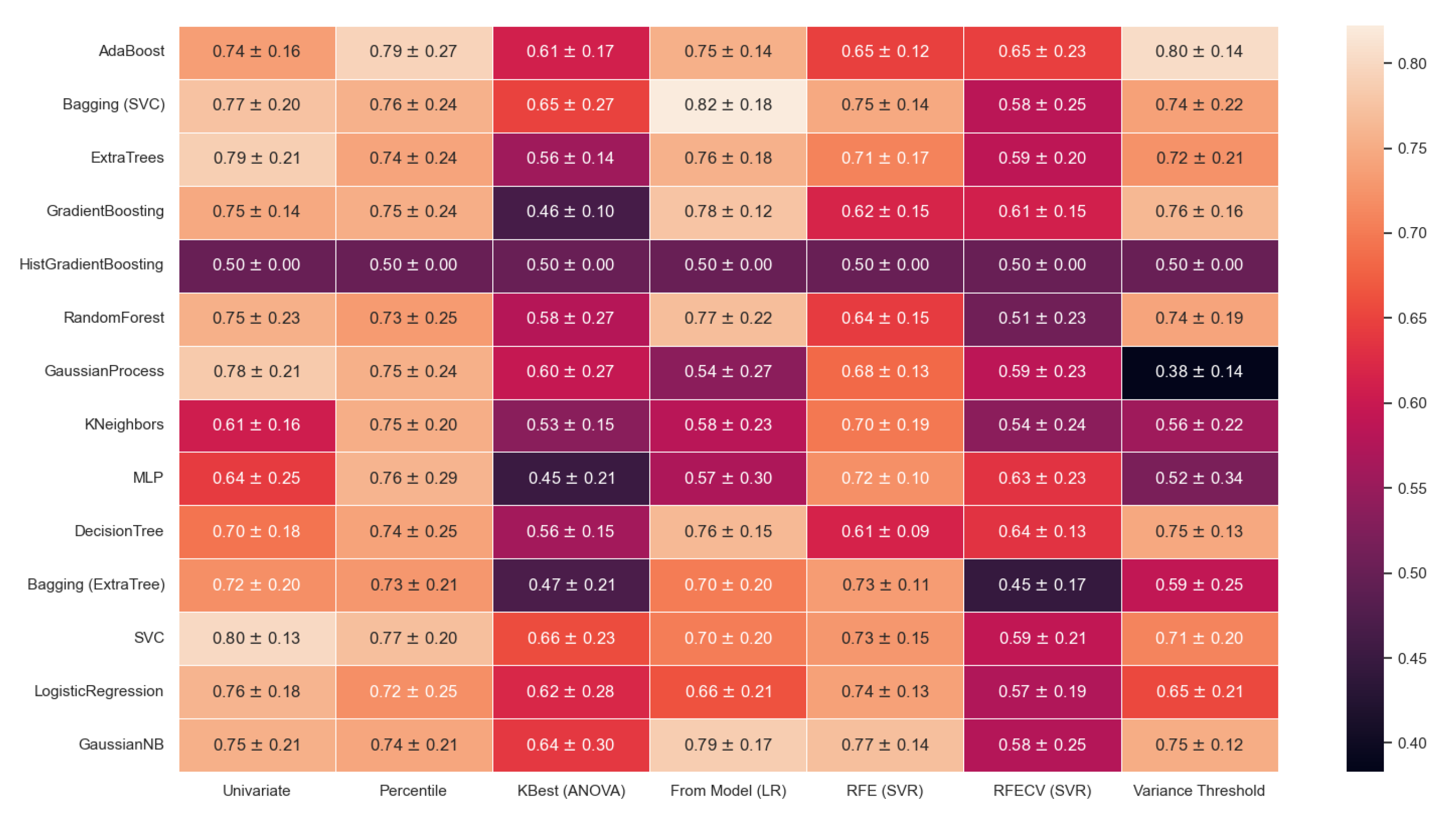
Figure 4 shows the obtained AUROC. 
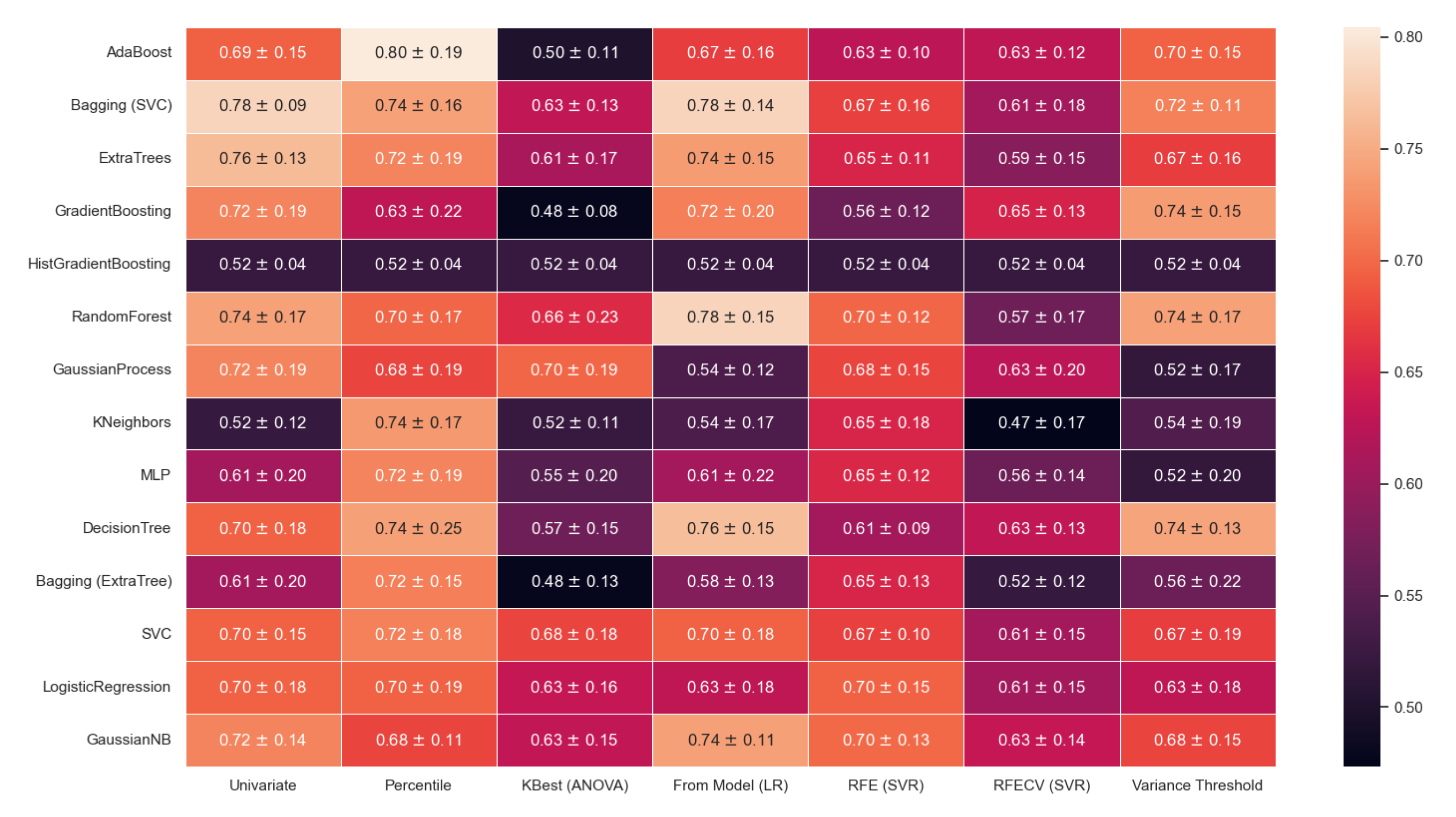
Figure 5 shows the obtained accuracy scores, and both present the corresponding mean standard deviations for the five fold cross-validation scheme (lighter colors mean a higher AUROC value as indicated in the color bar scale).
The pipelines were built with a very specific subset and goal - to distinguish favourable and unfavourable cases from PCa patients classified as intermediate risk. The specificity of this approach may provide EBRT with a tool capable of monitoring the true effectiveness of the treatment. An initial unfavourable outcome may become, during treatment, a favourable case, possibly leading to adjustments in the treatment workflow.
From the obtained results, a few pipelines do present good performance. In radiomic studies, there is always an issue with the reproducibility of the features. In the future, other CBCTs of each patient will be included in order to overcome this issue, as already performed by Bosetti et al. [12].
Still, results seem to suggest that some classifiers are not suited to this particular task. The HistGradientBoosting obtained an AUROC of 0.50 for every feature selection method. From the evaluated feature selection methods, the KBest (ANOVA) and RFECV (SVR) provided poor performances. On the other hand, the percentile feature selection method seems to have an overall decent performance, obtaining its best results when combined with an AdaBoost classifier with an AUROC of 0.79 ± 0.27 and its worst when combined with an LR classifier with an AUROC of 0.72 ± 0.25 .
Considering a threshold value of AUROC of 0.79, six pipelines were capable of obtaining good performance. Selecting features from an LR model and combining it with a Bagging (SVC) classifier or GaussianNB provided a pipeline with an AUROC value of 0.82 ± 0.18 and 0.79 ± 0.17 , respectively. Furthermore, the univariate selection method combined with an SVC obtained an AUROC of 0.80 ± 0.13 and, with an ExtraTrees, of 0.79 ± 0.21 . The Adaboost classifier combined with the baseline feature selection method, the variance threshold, provided an AUROC of 0.80 ± 0.14 , and when combined with the percentile feature selection method, an AUROC of 0.79 ± 0.27 . Table 6 highlights the selected pipelines obtained results.
The presented values are the mean values obtained for the five folds in the cross-validation. For these six pipelines, a deeper analysis was performed in order to evaluate the performance of each. Figure 6 presents the AUROC curves and corresponding values for each fold as well as the mean value. Furthermore, in grey, are the ± 1 standard deviation curves and, in dashed red, the 0.5 AUROC line.
In binary classification models, other metrics may provide valuable information on the performance of a classifier. The precision is defined as a ratio of the number of true positives divided by the sum of true positives and false positives. It is also referred to as the positive predictive power, this is, the ability of the model to predict true positives, which in this work, are the unfavourable cases (GG = 3). The recall (sensitivity) is calculated as the ratio of the number of true positives divided by the sum of true positives and false negatives. The f1-score is the harmonic mean of the precision and recall, while the support is the number of occurrences of each class in the ground truth labels [33]. Table 7 presents these parameters for the selected pipelines and the mean number of features selected in each fold in the cross-validation.
The threshold = 0, in the variance threshold method, is not enough to perform any feature selection because the preprocessing standardization removes the mean and scales features to unit variance. The AdaBoost classifier fits additional copies on the same dataset and re-adjusts the weights accordingly. This behaviour may overcome the lack of feature selection when both are combined. Besides the percentile–Adaboost combination, most pipelines present a low recall value for Class 2 (favourable), returning very few results. Themodel (LR)-bagging (SVC) pipeline has a high precision for Class 3 (unfavourable), suggesting those few results are well classified. This combination, however, has the opposite behaviour for Class 3. A high recall returns many results, but a low precision means those results are poorly classified.
The bagging (SVC) classifier aggregates the predictions of several SVCs, reducing the variance of the final output and improving accuracy. When using an SVC classifier, we obtained an accuracy of 0.0 ± 0.15 , but with a bagging strategy of 0.78 ± 0.14 . The GaussianNB classifier assumes a Gaussian likelihood with a naive assumption of pair-wise features’ conditional independence. By reducing the number of features to 43, we are also eliminating highly correlated features, a factor that degrades the classifier performance. The decision tree creates a piecewise constant approximation to the decision curve, but when using the entire feature set, the set is known to provide some overfitting. The ExtraTrees introduces randomized decision trees on several subsets allowing control of the overfitting and increasing accuracy [33].
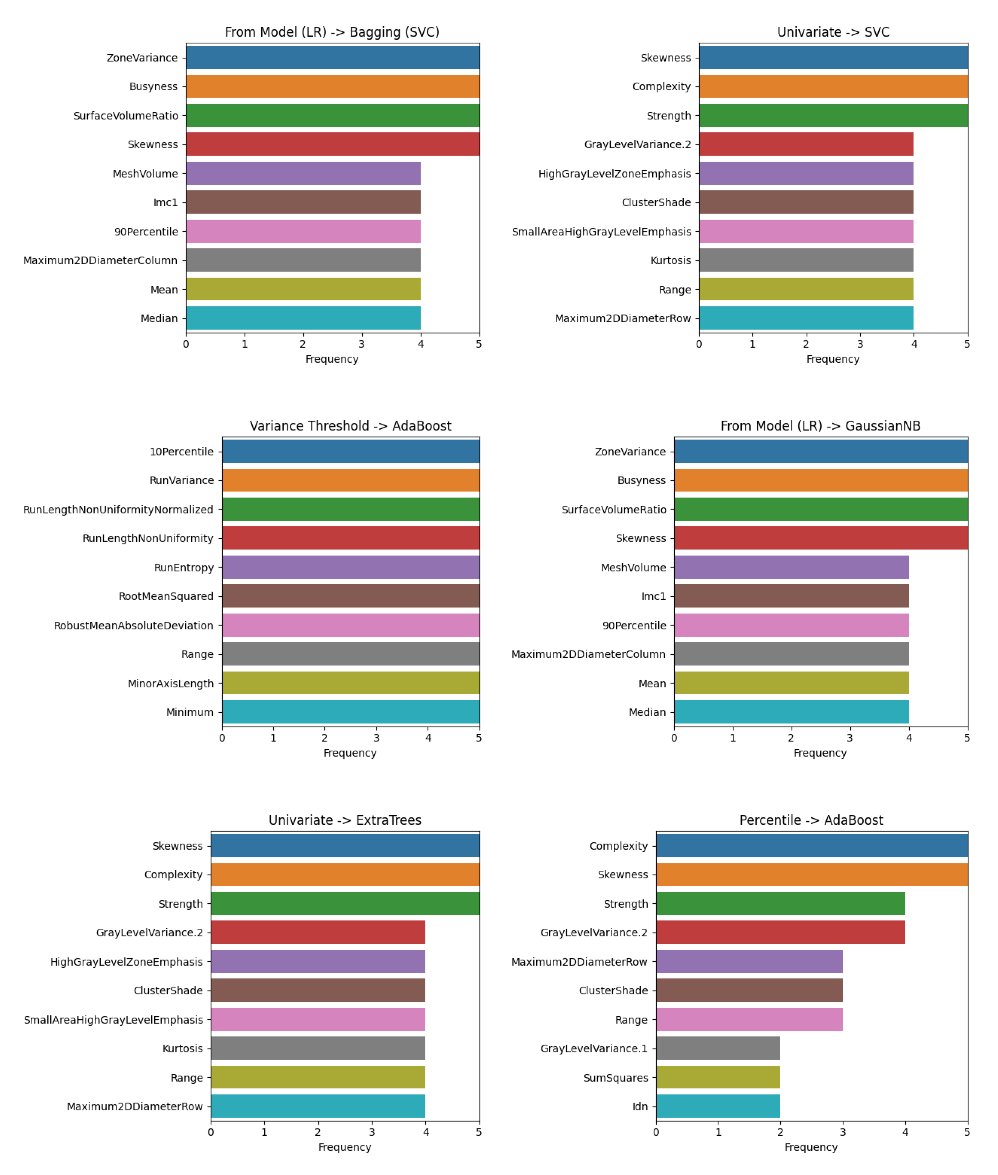
Percentile feature selection method with an AdaBoost classifier, the obtained results seem to be satisfactory, with relatively high values of precision and recall for both classes. The main advantage of this model is that the number of features used for classification is reduced to 11. This may be a step further in providing explainability and interpretability. In fact, the selected features in each fold of the cross-validation varies, although some are frequently selected. Figure 7 shows the features that were more frequently selected.
All evaluated feature selection methods select the skewness. Complexity features are selected using a univariate or percentile approach, while the zone variance, business and surface to volume ratio are selected when learning from an LR model. The percentile-AdaBoost pipeline is used the complexity and skewness features in the cross-validation. Increasing the number of folds in the cross-validation scheme may provide more valuable insights.

5. Conclusions

For PCa, EBRT is a curative option for localized and locally advanced disease and a palliative option for metastatic low-volume disease [6]. Currently, the only triggers for recurrence or treatment effectiveness monitoring are the PSA blood test or redoing a Transrectal Ultrasound Guided Biopsy (TRUS). With radiomics, a quantitative analysis of medical images may have similar prognostic power to phenotypes and gene protein signatures [9]. Interest in radiomics has been increasing and for PCa, it has been mainly focused on MRI in the initial staging and grading. However, during the EBRT, CBCTs are freely available, as they are used for patient positioning and setup verifications.
The value of CBCT-based radiomics was evaluated to distinguish between favourable and unfavourable prognosis for patients initially classified as intermediate risk. Such a tool may provide added value to monitor and trigger possible changes in EBRT outcomes. Following the current methods of feature selection and classification for PCa radiomics, 98 pipelines were evaluated. The results seem to suggest that selecting features from an LR model, combined with a bagging (SVC) classifier, provided good performance. Although using 43 features, it lacks the potential to offer explainability. In this sense, a better approach seems to be using a percentile feature selection method and an AdaBoost classifier. This pipeline presents an AUROC of 0.79 ± 0.27 and an accuracy of 0.80 ± 0.19 and high values of precision and recall, being the most balanced of the evaluated pipelines.
The skewness seems to be the most frequently selected feature, considering each fold in the cross-validation scheme. Although its true importance is yet to be evaluated, the fact it was selected in every fold of every feature selection method suggests it may provide some insights. Furthermore, the fact that only one CBCT was considered for each patient did not allow the evaluation of features reproducibility.
Although the obtained results are promising, some improvements need to be made for a deeper evaluation. A grid-search cross-validation may provide fine-tuning of parameters and improved results. Furthermore, the used subset is quite small, and may benefit in the future from the inclusion of high-risk patients and the assessment of other models.
CBCT-based radiomics may provide a baseline for an EBRT effectiveness assessment framework on ongoing treatment, improving outcomes and lowering recurrence rates regardless of the several limitations.

Author Contributions

Conceptualization, B.M.; methodology, B.M. and I.D.; software, B.M.; validation, B.M., I.D. and J.S.; formal analysis, B.M.; investigation, B.M.; resources, B.M., I.D., F.D. and J.S.; data curation, B.M. and F.D.; writing—original draft preparation, B.M.; writing—review and editing, B.M., I.D., F.D. and J.S.; supervision, I.D. and J.S. All authors have read and agreed to the published version of the manuscript.

Funding

This research received no external funding.

Institutional Review Board Statement

The study was conducted according to the guidelines of the Declaration of Helsinki. The study was approved by IPO Porto Healthcare Ethics Committee (protocol code CES.274/020 and date of approval 1 October 2020.

Informed Consent Statement

Informed consent was obtained from all subjects involved in the study.

Data Availability Statement

No new data were created or analyzed in this study. Data sharing is not applicable to this article.

Conflicts of Interest

The authors declare no conflict of interest.

Abbreviations

The following abbreviations are used in this manuscript:
ADCApparent Diffusion Coefficient
ANOVAAnalysis Of Variance
AUROC       Area Under the Receiver Operating Characteristic
BCRBiochemical Recurrence
BNBayesian Network
BPHBenign Prostatic Hyperplasia
CBCTCone Beam Computed Tomography
CTComputed Tomography
CTVClinical Target Volume
DREDigital Rectal Examination
EBRTExternal Beam Radiotherapy
GGGrade Group
GLCMGray Level Co-occurrence Matrix
GLDMGray Level Dependence Matrix
GLRLMGray Level Run Length Matrix
GLSZMGray Level Size Zone Matrix
GSGleason Score
GTVGross Tumor Volume
HUHounsfield Unit
IBSIImage Biomarker Standardisation Initiative
ICRUInternational Commission on Radiation Units and Measurements
IMRTIntensity Modulated Radiation Therapy
IPO-PORTOInstituto Português de Oncologia do Porto Francisco Gentil
KNNK-nearest Neighbors
LIFExLocal Image Features Extraction
LINACMedical Linear Accelerator
LRLinear Regression
mpMRImulti-parametric Magnetic Ressonance Imaging
MRIMagnetic Ressonance Imaging
NGTDMNeighbouring Gray Tone Difference Matrix
NNNeural Network
PCAPrincipal Component Analysis
PCaProstate Cancer
PETPositron Emission Tomography
PIRADSProstate Imaging Reporting and Data System
PSAProstate Specific Antigen
RFRandom Forest
RFERecursive Feature Elimination
RGRisk Group
ROIRegion Of Interest
SVCSupport Vector Classifier
SVMSupport Vector Machine
TBTree Based
TRUSTransrectal Ultrasound Guided Biopsy
XGBExtreme Gradient Boosting

References

  1. Sung, H.; Ferlay, J.; Siegel, R.L.; Laversanne, M.; Soerjomataram, I.; Jemal, A.; Bray, F. Global Cancer Statistics 2020: GLOBOCAN Estimates of Incidence and Mortality Worldwide for 36 Cancers in 185 Countries. CA A Cancer J. Clin. 2021, 71, 209–249. [Google Scholar] [CrossRef] [PubMed]
  2. Singh, V. Textbook of Anatomy: Abdomen and Lower Limb; 3rd Updated Edition-EBook; Elsevier: New Delhi, India, 2020; Volume 2. [Google Scholar]
  3. Humphrey, P.A. Histopathology of prostate cancer. Cold Spring Harb. Perspect. Med. 2017, 7, a030411. [Google Scholar] [CrossRef] [PubMed] [Green Version]
  4. DeMarzo, A.M.; Nelson, W.G.; Isaacs, W.B.; Epstein, J.I. Pathological and molecular aspects of prostate cancer. Lancet 2003, 361, 955–964. [Google Scholar] [CrossRef] [PubMed]
  5. Epstein, J.I.; Egevad, L.; Amin, M.B.; Delahunt, B.; Srigley, J.R.; Humphrey, P.A. The 2014 International Society of Urological Pathology (ISUP) consensus conference on Gleason grading of prostatic carcinoma. Am. J. Surg. Pathol. 2016, 40, 244–252. [Google Scholar] [CrossRef]
  6. Parker, C.; Castro, E.; Fizazi, K.; Heidenreich, A.; Ost, P.; Procopio, G.; Tombal, B.; Gillessen, S. Prostate cancer: ESMO Clinical Practice Guidelines for diagnosis, treatment and follow-up. Ann. Oncol. 2020, 31, 1119–1134. [Google Scholar] [CrossRef]
  7. Schröder, F.H.; Kruger, A.B.; Rietbergen, J.; Kranse, R.; Maas, P.v.d.; Beemsterboer, P.; Hoedemaeker, R. Evaluation of the digital rectal examination as a screening test for prostate cancer. J. Natl. Cancer Inst. 1998, 90, 1817–1823. [Google Scholar] [CrossRef] [Green Version]
  8. Klotz, L. Active surveillance for prostate cancer: For whom? J. Clin. Oncol. 2005, 23, 8165–8169. [Google Scholar] [CrossRef]
  9. Gillies, R.J.; Kinahan, P.E.; Hricak, H. Radiomics: Images are more than pictures, they are data. Radiology 2016, 278, 563–577. [Google Scholar] [CrossRef] [Green Version]
  10. Van Griethuysen, J.J.; Fedorov, A.; Parmar, C.; Hosny, A.; Aucoin, N.; Narayan, V.; Beets-Tan, R.G.; Fillion-Robin, J.C.; Pieper, S.; Aerts, H.J. Computational radiomics system to decode the radiographic phenotype. Cancer Res. 2017, 77, e104–e107. [Google Scholar] [CrossRef] [Green Version]
  11. Mendes, B.; Domingues, I.; Silva, A.; Santos, J. Prostate Cancer Aggressiveness Prediction Using CT Images. Life 2021, 11, 1164. [Google Scholar] [CrossRef]
  12. Bosetti, D.G.; Ruinelli, L.; Piliero, M.A.; van der Gaag, L.C.; Pesce, G.A.; Valli, M.; Bosetti, M.; Presilla, S.; Richetti, A.; Deantonio, L. Cone-beam computed tomography-based radiomics in prostate cancer: A mono-institutional study. Strahlenther. Und Onkol. 2020, 196, 943–951. [Google Scholar] [CrossRef]
  13. Lambin, P.; Rios-Velazquez, E.; Leijenaar, R.; Carvalho, S.; Van Stiphout, R.G.; Granton, P.; Zegers, C.M.; Gillies, R.; Boellard, R.; Dekker, A.; et al. Radiomics: Extracting more information from medical images using advanced feature analysis. Eur. J. Cancer 2012, 48, 441–446. [Google Scholar] [CrossRef] [Green Version]
  14. Yao, S.; Jiang, H.; Song, B. Radiomics in prostate cancer: Basic concepts and current state-of-the-art. Chin. J. Acad. Radiol. 2020, 2, 47–55. [Google Scholar] [CrossRef] [Green Version]
  15. Min, X.; Li, M.; Dong, D.; Feng, Z.; Zhang, P.; Ke, Z.; You, H.; Han, F.; Ma, H.; Tian, J.; et al. Multi-parametric MRI-based radiomics signature for discriminating between clinically significant and insignificant prostate cancer: Cross-validation of a machine learning method. Eur. J. Radiol. 2019, 115, 16–21. [Google Scholar] [CrossRef] [Green Version]
  16. Hou, Y.; Bao, M.L.; Wu, C.J.; Zhang, J.; Zhang, Y.D.; Shi, H.B. A radiomics machine learning-based redefining score robustly identifies clinically significant prostate cancer in equivocal PI-RADS score 3 lesions. Abdom. Radiol. 2020, 45, 4223–4234. [Google Scholar] [CrossRef]
  17. Woźnicki, P.; Westhoff, N.; Huber, T.; Riffel, P.; Froelich, M.F.; Gresser, E.; von Hardenberg, J.; Mühlberg, A.; Michel, M.S.; Schoenberg, S.O.; et al. Multiparametric MRI for prostate cancer characterization: Combined use of radiomics model with PI-RADS and clinical parameters. Cancers 2020, 12, 1767. [Google Scholar] [CrossRef]
  18. Bernatz, S.; Ackermann, J.; Mandel, P.; Kaltenbach, B.; Zhdanovich, Y.; Harter, P.N.; Döring, C.; Hammerstingl, R.; Bodelle, B.; Smith, K.; et al. Comparison of machine learning algorithms to predict clinically significant prostate cancer of the peripheral zone with multiparametric MRI using clinical assessment categories and radiomic features. Eur. Radiol. 2020, 30, 6757–6769. [Google Scholar] [CrossRef]
  19. Li, M.; Chen, T.; Zhao, W.; Wei, C.; Li, X.; Duan, S.; Ji, L.; Lu, Z.; Shen, J. Radiomics prediction model for the improved diagnosis of clinically significant prostate cancer on biparametric MRI. Quant. Imaging Med. Surg. 2020, 10, 368. [Google Scholar] [CrossRef]
  20. Bevilacqua, A.; Mottola, M.; Ferroni, F.; Rossi, A.; Gavelli, G.; Barone, D. The Primacy of High B-Value 3T-DWI Radiomics in the Prediction of Clinically Significant Prostate Cancer. Diagnostics 2021, 11, 739. [Google Scholar] [CrossRef]
  21. Bleker, J.; Kwee, T.C.; Dierckx, R.A.; de Jong, I.J.; Huisman, H.; Yakar, D. Multiparametric MRI and auto-fixed volume of interest-based radiomics signature for clinically significant peripheral zone prostate cancer. Eur. Radiol. 2020, 30, 1313–1324. [Google Scholar] [CrossRef]
  22. Abraham, B.; Nair, M.S. Computer-aided classification of prostate cancer grade groups from MRI images using texture features and stacked sparse autoencoder. Comput. Med. Imaging Graph. 2018, 69, 60–68. [Google Scholar] [CrossRef] [PubMed]
  23. Algohary, A.; Shiradkar, R.; Pahwa, S.; Purysko, A.; Verma, S.; Moses, D.; Shnier, R.; Haynes, A.M.; Delprado, W.; Thompson, J.; et al. Combination of peri-tumoral and intra-tumoral radiomic features on bi-parametric MRI accurately stratifies prostate cancer risk: A multi-site study. Cancers 2020, 12, 2200. [Google Scholar] [CrossRef] [PubMed]
  24. Cysouw, M.C.; Jansen, B.H.; van de Brug, T.; Oprea-Lager, D.E.; Pfaehler, E.; de Vries, B.M.; van Moorselaar, R.J.; Hoekstra, O.S.; Vis, A.N.; Boellaard, R. Machine learning-based analysis of [18 F] DCFPyL PET radiomics for risk stratification in primary prostate cancer. Eur. J. Nucl. Med. Mol. Imaging 2021, 48, 340–349. [Google Scholar] [CrossRef] [PubMed]
  25. Alongi, P.; Stefano, A.; Comelli, A.; Laudicella, R.; Scalisi, S.; Arnone, G.; Barone, S.; Spada, M.; Purpura, P.; Bartolotta, T.V.; et al. Radiomics analysis of 18F-Choline PET/CT in the prediction of disease outcome in high-risk prostate cancer: An explorative study on machine learning feature classification in 94 patients. Eur. Radiol. 2021, 31, 4595–4605. [Google Scholar] [CrossRef] [PubMed]
  26. Osman, S.O.; Leijenaar, R.T.; Cole, A.J.; Lyons, C.A.; Hounsell, A.R.; Prise, K.M.; O’Sullivan, J.M.; Lambin, P.; McGarry, C.K.; Jain, S. Computed tomography-based radiomics for risk stratification in prostate cancer. Int. J. Radiat. Oncol. Biol. Phys. 2019, 105, 448–456. [Google Scholar] [CrossRef]
  27. Nioche, C.; Orlhac, F.; Boughdad, S.; Reuzé, S.; Goya-Outi, J.; Robert, C.; Pellot-Barakat, C.; Soussan, M.; Frouin, F.; Buvat, I. LIFEx: A freeware for radiomic feature calculation in multimodality imaging to accelerate advances in the characterization of tumor heterogeneity. Cancer Res. 2018, 78, 4786–4789. [Google Scholar] [CrossRef] [Green Version]
  28. ICRU. Prescribing, recording, and reporting photon-beam intensity-modulated radiation therapy (IMRT). J. Int. Comm. Radiat. Units Meas. (JICRU) 2010, 10, 41–53. [Google Scholar]
  29. Klein, S.; Staring, M.; Murphy, K.; Viergever, M.A.; Pluim, J.P. Elastix: A toolbox for intensity-based medical image registration. IEEE Trans. Med. Imaging 2009, 29, 196–205. [Google Scholar] [CrossRef]
  30. Shamonin, D.P.; Bron, E.E.; Lelieveldt, B.P.; Smits, M.; Klein, S.; Staring, M.; Initiative, A.D.N. Fast parallel image registration on CPU and GPU for diagnostic classification of Alzheimer’s disease. Front. Neuroinform. 2014, 7, 50. [Google Scholar] [CrossRef] [Green Version]
  31. Fedorov, A.; Beichel, R.; Kalpathy-Cramer, J.; Finet, J.; Fillion-Robin, J.C.; Pujol, S.; Bauer, C.; Jennings, D.; Fennessy, F.; Sonka, M.; et al. 3D Slicer as an image computing platform for the Quantitative Imaging Network. Magn. Reson. Imaging 2012, 30, 1323–1341. [Google Scholar] [CrossRef] [Green Version]
  32. Zwanenburg, A.; Vallières, M.; Abdalah, M.A.; Aerts, H.J.; Andrearczyk, V.; Apte, A.; Ashrafinia, S.; Bakas, S.; Beukinga, R.J.; Boellaard, R.; et al. The image biomarker standardization initiative: Standardized quantitative radiomics for high-throughput image-based phenotyping. Radiology 2020, 295, 328. [Google Scholar] [CrossRef]
  33. Pedregosa, F.; Varoquaux, G.; Gramfort, A.; Michel, V.; Thirion, B.; Grisel, O.; Blondel, M.; Prettenhofer, P.; Weiss, R.; Dubourg, V.; et al. Scikit-learn: Machine Learning in Python. J. Mach. Learn. Res. 2011, 12, 2825–2830. [Google Scholar] [CrossRef]
  34. Bourbonne, V.; Fournier, G.; Vallières, M.; Lucia, F.; Doucet, L.; Tissot, V.; Cuvelier, G.; Hue, S.; Le Penn Du, H.; Perdriel, L.; et al. External validation of an MRI-derived radiomics model to predict biochemical recurrence after surgery for high-risk prostate cancer. Cancers 2020, 12, 814. [Google Scholar] [CrossRef] [Green Version]
  35. Chen, A.; Zhu, L.; Zang, H.; Ding, Z.; Zhan, S. Computer-aided diagnosis and decision-making system for medical data analysis: A case study on prostate MR images. J. Manag. Sci. Eng. 2019, 4, 266–278. [Google Scholar] [CrossRef]
  36. Toivonen, J.; Montoya Perez, I.; Movahedi, P.; Merisaari, H.; Pesola, M.; Taimen, P.; Boström, P.J.; Pohjankukka, J.; Kiviniemi, A.; Pahikkala, T.; et al. Radiomics and machine learning of multisequence multiparametric prostate MRI: Towards improved non-invasive prostate cancer characterization. PLoS ONE 2019, 14, e0217702. [Google Scholar] [CrossRef] [Green Version]
  37. Wildeboer, R.R.; van Sloun, R.J.; Huang, P.; Wijkstra, H.; Mischi, M. 3-D multi-parametric contrast-enhanced ultrasound for the prediction of prostate cancer. Ultrasound Med. Biol. 2019, 45, 2713–2724. [Google Scholar] [CrossRef]
  38. Abdollahi, H.; Mofid, B.; Shiri, I.; Razzaghdoust, A.; Saadipoor, A.; Mahdavi, A.; Galandooz, H.M.; Mahdavi, S.R. Machine learning-based radiomic models to predict intensity-modulated radiation therapy response, Gleason score and stage in prostate cancer. La Radiol. Medica 2019, 124, 555–567. [Google Scholar] [CrossRef]
  39. Cuocolo, R.; Stanzione, A.; Faletti, R.; Gatti, M.; Calleris, G.; Fornari, A.; Gentile, F.; Motta, A.; Dell’Aversana, S.; Creta, M.; et al. MRI index lesion radiomics and machine learning for detection of extraprostatic extension of disease: A multicenter study. Eur. Radiol. 2021, 31, 7575–7583. [Google Scholar] [CrossRef]
  40. Shiradkar, R.; Ghose, S.; Jambor, I.; Taimen, P.; Ettala, O.; Purysko, A.S.; Madabhushi, A. Radiomic features from pretreatment biparametric MRI predict prostate cancer biochemical recurrence: Preliminary findings. J. Magn. Reson. Imaging 2018, 48, 1626–1636. [Google Scholar] [CrossRef]
  41. Castillo T, J.M.; Starmans, M.P.; Arif, M.; Niessen, W.J.; Klein, S.; Bangma, C.H.; Schoots, I.G.; Veenland, J.F. A multi-center, multi-vendor study to evaluate the generalizability of a radiomics model for classifying prostate cancer: High grade vs. low grade. Diagnostics 2021, 11, 369. [Google Scholar] [CrossRef]
  42. Murakami, Y.; Magome, T.; Mizutani, T.; Sato, T.; Yoshioka, Y.; Oguchi, M. Potential of Radiomic Feature Related to Prostatic Calcifications for the Machine Learning-Based Prediction of Biochemical Recurrence in Prostate Cancer Patient. Int. J. Radiat. Oncol. Biol. Phys. 2019, 105, E137. [Google Scholar] [CrossRef]
  43. Stanzione, A.; Cuocolo, R.; Cocozza, S.; Romeo, V.; Persico, F.; Fusco, F.; Longo, N.; Brunetti, A.; Imbriaco, M. Detection of extraprostatic extension of cancer on biparametric MRI combining texture analysis and machine learning: Preliminary results. Acad. Radiol. 2019, 26, 1338–1344. [Google Scholar] [CrossRef] [PubMed]
  44. Xu, M.; Fang, M.; Zou, J.; Yang, S.; Yu, D.; Zhong, L.; Hu, C.; Zang, Y.; Dong, D.; Tian, J.; et al. Using biparametric MRI radiomics signature to differentiate between benign and malignant prostate lesions. Eur. J. Radiol. 2019, 114, 38–44. [Google Scholar] [CrossRef] [PubMed]
  45. Liang, L.; Zhi, X.; Sun, Y.; Li, H.; Wang, J.; Xu, J.; Guo, J. A Nomogram Based on a Multiparametric Ultrasound Radiomics Model for Discrimination between Malignant and Benign Prostate Lesions. Front. Oncol. 2021, 11, 290. [Google Scholar] [CrossRef]
Figure 1. Radiomic studies pipeline.
Applsci 13 01378 g001
Figure 2. Initial CT scan with manually drawn prostate (yellow) and registered CBCT. (a) Initial CT scan. (b) First EBRT session CBCT.
Applsci 13 01378 g002
Figure 3. Pipeline evaluation flowchart.
Applsci 13 01378 g003
Figure 4. ROC values with a five fold-CV.
Applsci 13 01378 g004
Figure 5. Accuracy values with a 5-fold CV.
Applsci 13 01378 g005
Figure 6. ROC curves obtained for the selected pipelines.
Applsci 13 01378 g006
Figure 7. Selected features frequency.
Applsci 13 01378 g007
Table 1. Acquisition settings for CBCT.
LINACkVp (kV)Pixel Spacing (mm × mm)Slice Thickness (mm)
NOVALIS125 0.879 × 0.879 / 1.172 × 1.172 2.500/2.000
TRUEBEAM140/125 0.908 × 0.908 1.988
TRILOGY125 0.879 × 0.879 2.500
Table 2. Patients Stratification.
GSRGGG# of Cases
3+3Low/very low12
3+4Intermediate (favourable)222
4+3Intermediate (unfavourable)324
4+4High414
4+5/5+4Very high58
Table 3. Extracted radiomics feature classes.
Feature Class# Features
Shape-based14
First order18
GLCM24
GLDM14
GLRLM16
GLSZM16
NGTDM5
Total107
Table 4. Evaluated feature selection methods.
GroupNameParameters
StatisticsUnivariateK-best → k = 20
PercentilePercentile = 10
KBest (ANOVA)K-best → k = 5
From estimatorFrom model (LR)Penalty = “l2”; C = 1
RFE (SVR)SVR (kernel = “linear”); n_features = 3
RFECV (SVR)SVR (kernel = “linear”); cv = 5
BaselineVariance thresholdThreshold = 0
Table 5. Evaluated Classifiers.
NameParameters
AdaBoostn_estimators = 100
Bagging (SVC)base_estimator = SVC(), n_estimators = 10
ExtraTreesn_estimators = 100
GradientBoostingn_estimators = 100; learning_rate = 1.0; max_depth = 1
HistGradientBoostingloss = “log_loss”
RandomForestmax_depth = 2
GaussianProcesskernel = 1.0 * Radial-basis function(1.0)
KNeighborsn_neighbors = 3
MLPhidden_layer_sizes = (100, ); activation = “relu”; solver = “adam”
DecisionTreecriterion = “gini”; splitter = “best”
Bagging (ExtraTree)base_estimator = ExtraTreeClassifier()
SVCkernel = “linear”
LogisticRegressionpenalty = “l2”; C = 1
GaussianNBvar_smoothing = 1 × 10 9
Table 6. Selected pipelines results ordered by AUROC.
Feature SelectionClassifierAUROCAccuracy Score
From model (LR)Bagging (SVC) 0.82 ± 0.18 0.78 ± 0.14
UnivariateSVC 0.80 ± 0.13 0.70 ± 0.15
Variance thresholdAdaboost 0.80 ± 0.14 0.70 ± 0.15
From model (LR)GaussianNB 0.79 ± 0.17 0.74 ± 0.11
UnivariateExtraTrees 0.79 ± 0.21 0.76 ± 0.13
PercentileAdaBoost 0.79 ± 0.27 0.80 ± 0.19
Table 7. Best pipelines’ performance parameters.
SelectorClassifierClassPrecisionRecallf1-ScoreSupportFeatures
Model (LR)Bagging (SVC)2 0.90 ± 0.20 0.64 ± 0.16 0.73 ± 0.16 4.40 ± 0.49 43
3 0.74 ± 0.10 0.92 ± 0.16 0.82 ± 0.12 4.80 ± 0.40
UnivariateSVC2 0.68 ± 0.17 0.64 ± 0.24 0.65 ± 0.20 4.40 ± 0.49 20
3 0.71 ± 0.17 0.75 ± 0.08 0.73 ± 0.12 4.80 ± 0.40
Variance thresholdAdaBoost2 0.70 ± 0.22 0.64 ± 0.24 0.65 ± 0.20 4.40 ± 0.49 107
3 0.72 ± 0.16 0.76 ± 0.15 0.73 ± 0.12 4.80 ± 0.40
Model (LR)Gaussian NB2 0.81 ± 0.19 0.64 ± 0.16 0.70 ± 0.14 4.40 ± 0.49 43
3 0.72 ± 0.09 0.83 ± 0.15 0.77 ± 0.10 4.80 ± 0.40
UnivariateExtraTrees2 0.85 ± 0.20 0.64 ± 0.16 0.71 ± 0.15 4.40 ± 0.49 20
3 0.73 ± 0.10 0.88 ± 0.16 0.79 ± 0.11 4.80 ± 0.40
PercentileAdaBoost2 0.80 ± 0.22 0.82 ± 0.22 0.79 ± 0.19 4.40 ± 0.49 11
3 0.84 ± 0.20 0.80 ± 0.22 0.81 ± 0.19 4.80 ± 0.40
Disclaimer/Publisher’s Note: The statements, opinions and data contained in all publications are solely those of the individual author(s) and contributor(s) and not of MDPI and/or the editor(s). MDPI and/or the editor(s) disclaim responsibility for any injury to people or property resulting from any ideas, methods, instructions or products referred to in the content.

