Toward the Design of a Representative Heater for Boiling Flow Characterization under PWR’s Prototypical Thermalhydraulic Conditions

Featured Application

This work is related to boiling studies in PWR conditions, it will lead to the design of an experimental setup to characterise boiling flow and develop safety models over boiling crisis.

Abstract

In order to improve the understanding of the phenomena underlying the boiling occurrence, CEA Cadarache (France) is designing a new experimental setup, intended to operate for pressures ranging from atmospheric to PWR conditions. This will allow optical access to the convective boiling flow as well as thermal imaging (infrared thermography) of the heated surface. A two-step methodology for designing the heater (particularly its thickness since it directly influences the boiling mechanisms) was developed. This approach is based on solving the heat conduction problem within the heater, considering realistic time-dependent boundary conditions representative of the boiling process. Since those boundary conditions are measured on the external face of the heater, this heat transfer problem is known as an inverse problem that is difficult to solve because of its ill-posedness and high sensitivity to boundary condition uncertainties. In the first stage, we considered one-dimensional modeling to determine the order of magnitude of the heater’s thickness that guaranteed a correct reconstruction of the wet temperature from the measured dry temperature in terms of uncertainties. This value was confirmed in the second stage using a two-dimensional model that accounted for the presence of multiple bubbles on the wet side.

1. Introduction

In nuclear power plants, boiling occurrence on the fuel assembly can lead to a boiling crisis and damage some fuel elements within the core assembly. It is then an important matter to be able to determine the conditions leading to DNB (departure from nucleate boiling) as accurately as possible. It is believed that such a goal will require a better understanding of the physical mechanisms driving the nucleate boiling phenomena. The purpose of this work is to study and characterize nucleate boiling from the onset of nucleate boiling (ONB) up to the boiling crisis triggering, under working conditions that are prototypical of PWR (pressurized water reactor) thermal-hydraulic operating conditions. PWR’s primary circuit is characterized by a pressure of 155 bar, a temperature close to 300 ${}^{\circ }$C, and a flow rate of 68,350 m${}^3$/h.

In terms of modeling, nucleate boiling is often described in CFD tools (NEPTUNE CFD, Fluent) using the heat flux wall partitioning approach as first introduced by Kurul and Podowski [1]. This model assumes that the wall heat flux $q_w^{"}$ can be divided in three components—the evaporation heat flux $q_e^{"}$, the quenching heat flux $q_q^{"}$, and the single-phase convective heat flux $q_c^{"}$, respectively (see Figure 1).

The evaporation heat flux depends on three parameters—the nucleation site density $N^{″}$, the bubble departure frequency f, and the lift-off bubble diameter $D_b$. These parameters are often provided by different correlations [2,3]. Unfortunately, there are two main drawbacks.

First, most of those correlations are based on experimental measurements performed at low pressure and low-temperature conditions or for different working fluids (refrigerant, e.g., R12, R134a, R113). For instance, the bubble diameter $D_b$ is often determined using the well-known correlation by Unal [3]. Despite this correlation often being used for high-pressure and high-temperature steam/water flows [4], one should notice that the high-pressure database for this correlation is based on the De Munk experiments, which were performed with sodium [5]. Considering this correlation is dimensional, it is legitimate to wonder about the applicability of this sub-model to PWR thermal-hydraulic conditions.

Secondly, those parameters were not simultaneously measured during the experiments. This means that from a practical point of view, two parameters were measured (for example the bubble diameter $D_b$ and the bubble detachment frequency f) and the remaining parameter (in this example, the nucleation site density $N^{″}$) was fitted by comparing the model prediction to some secondary experimental measurements, such as the wall temperature or the void fraction. This approach may be risky because even if the final calculations seem to be consistent, they may result from error compensations within the model.

To ensure the validity of the partitioning model, it seems necessary to perform direct and complete measurements of all the sub-model parameters in the operating conditions as close as possible to the targeted ones (PWR).

To achieve this goal, it is worth mentioning the work of Richenderfer et al. [6], who designed an experimental setup that allows measurements of each parameter mentioned above (bubble diameter $D_b$, bubble detachment frequency f, and nucleation site density $N^{″}$). This setup is made of a test section (square cross-sectional) equipped with quartz windows to obtain optical access to the flow. The heater (where nucleate boiling occurs, see Figure 2) is made of a sapphire plate (substrate) coated with a thin layer of indium-tin oxide (ITO). The thickness of this ITO coating is 0.7 µm and is heated by the direct Joule effect.

They managed to visualize the bubbles through the sapphire beneath the heater and collect the data related to the heated plate temperature and heat flux. An infra-red high-speed camera measures the temperature of the heated plate on its external face and the temperature of the wet side of the plate is obtained by solving an inverse conduction–radiation problem–solution.

Despite the obvious interest in such an experiment, the representativeness of the heated surface is questionable, in particular, due to its thickness. One should notice that for classical industrial plates (e.g., metallic plates), the characteristic size of an active nucleation site is of the same order of magnitude, not to say larger, than the thickness of the ITO layer used by Richenderfer et al. [6]. This may influence the correct development of a bubble.

To illustrate this influence, let us consider the work of March [4]. He designed an experimental setup to study the two-phase flow characteristics for PWR thermal-hydraulic conditions. The test section was composed of a rod bundle with nine rods heated by the direct Joule effect. Those rods were placed inside a vessel that could support the pressure. The vessel was equipped with two sapphire windows that allowed direct visualization of the two-phase flow along the heated rods, particularly the bubbles that were created at the surface of the rods. Pictures of the flow were obtained using shadowgraphy. Experiments were performed within the following thermal-hydraulic parameter range (i) pressure from 26 bars up to 155 bars, (ii) mass velocity ranging from 1000 to 3500 kg·m${}^{-2}$·s${}^{-1}$, and (iii) equilibrium exit quality $x_{eq}$ corresponding to sub-cooled conditions (from ONB up to $x_{eq}\approx 0$, where $x_{eq}$ is defined by $x_{eq}=\frac{h_m-h_{l,sat}}{h_{lv}}$, where $h_{lv}$ is the latent heat and $h_{l,sat}$ is the saturated liquid enthalpy).

During the tests, March [4] focused on the impact of the roughness of the heated surface on nucleate boiling (especially the sizes of the bubbles). He observed strong changes in the flow structure, especially in the bubble size as a function of the roughness. For a smooth surface, which can be characterized by a roughness close to 0.2 µm, and for the same set of thermal-hydraulic conditions, the bubbles are quite larger than the bubbles created at the surface of the rough rod (characterized by a higher roughness close to 3.9 µm). It appears that the roughness largely influences the nature of the boiling flow, particularly in terms of bubble size [7]. This result confirms that it is necessary to consider a realistically heated plate in order to ensure good representativeness.

If March’s work [4] clearly demonstrates the technical feasibility of such measurements, some limitations should be pointed out. The influence of optical distortion due to the thermal gradient (refractive index) in the vicinity of the heated wall was not studied and very little data were collected. The resulting database needs to be completed. One can also notice that there were no thermal measurements concerning the heater. Finally, to the best of our knowledge, data collected by March [4] were unique but have not been challenged by anyone else; moreover, reproducibility still needs to be demonstrated.

The main objective of the present work was to design a setup to measure the previously mentioned parameters for operating conditions that are representative of a pressurized water reactor and, therefore, extend the initial work performed by March [4]. A realistic heater needs to be designed, taking into account the previous work described ahead. To achieve this goal, a specific study of the thermal behavior of the heater is presented. This study will lead to the determination of the heater thickness, which is believed to be the most influential parameter in our problem.

This paper is organized as follows:

• The experimental setup and associated measurement techniques are introduced in the Section 2.
• The thermal behavior of the heater is then studied through a 1D approach considering realistic time-dependent boundary conditions that properly simulate nucleate boiling in Section 3.
• In the Section 4, a 2D extension analysis of the thermal behavior of the heater is introduced; some discussions concerning space meshing of the method and enhancement will be presented.
• Finally, the Section 5 concludes this study by highlighting the main findings and suggestions for further research.

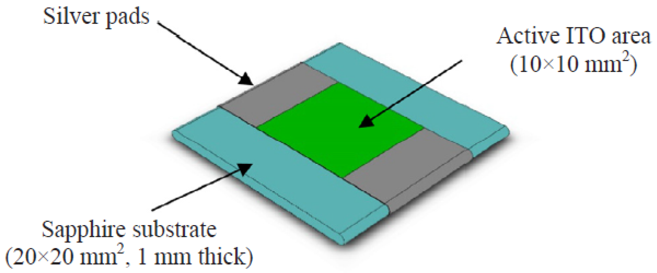
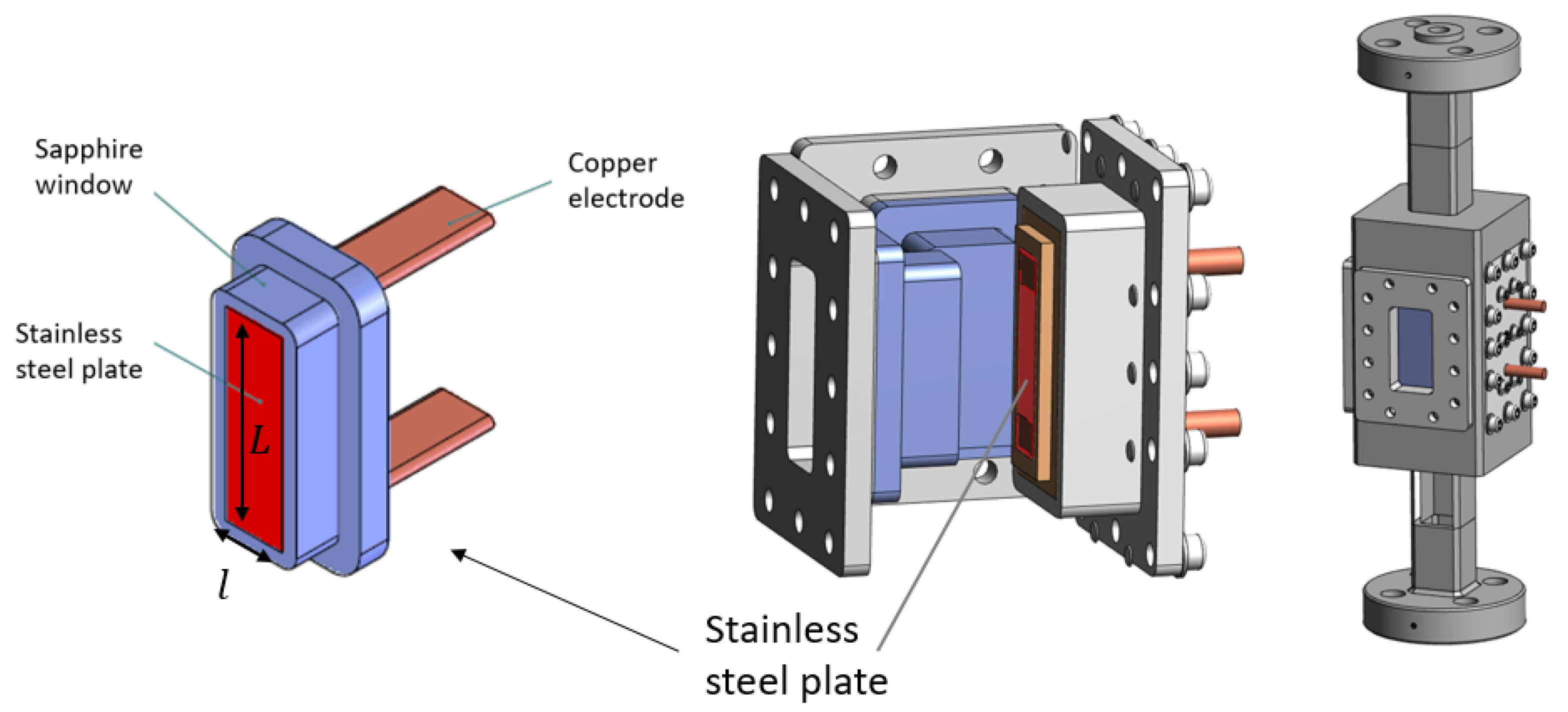
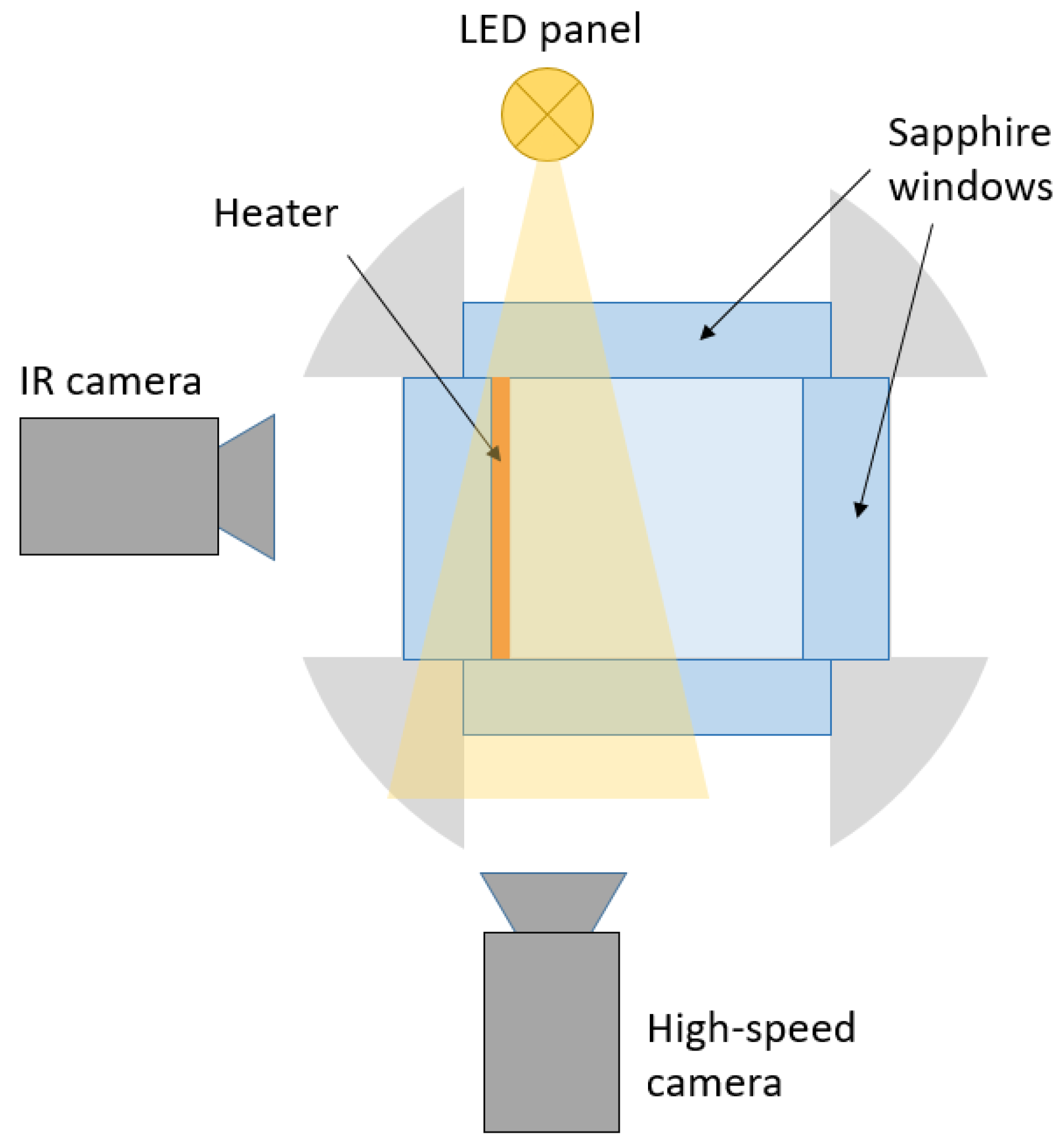
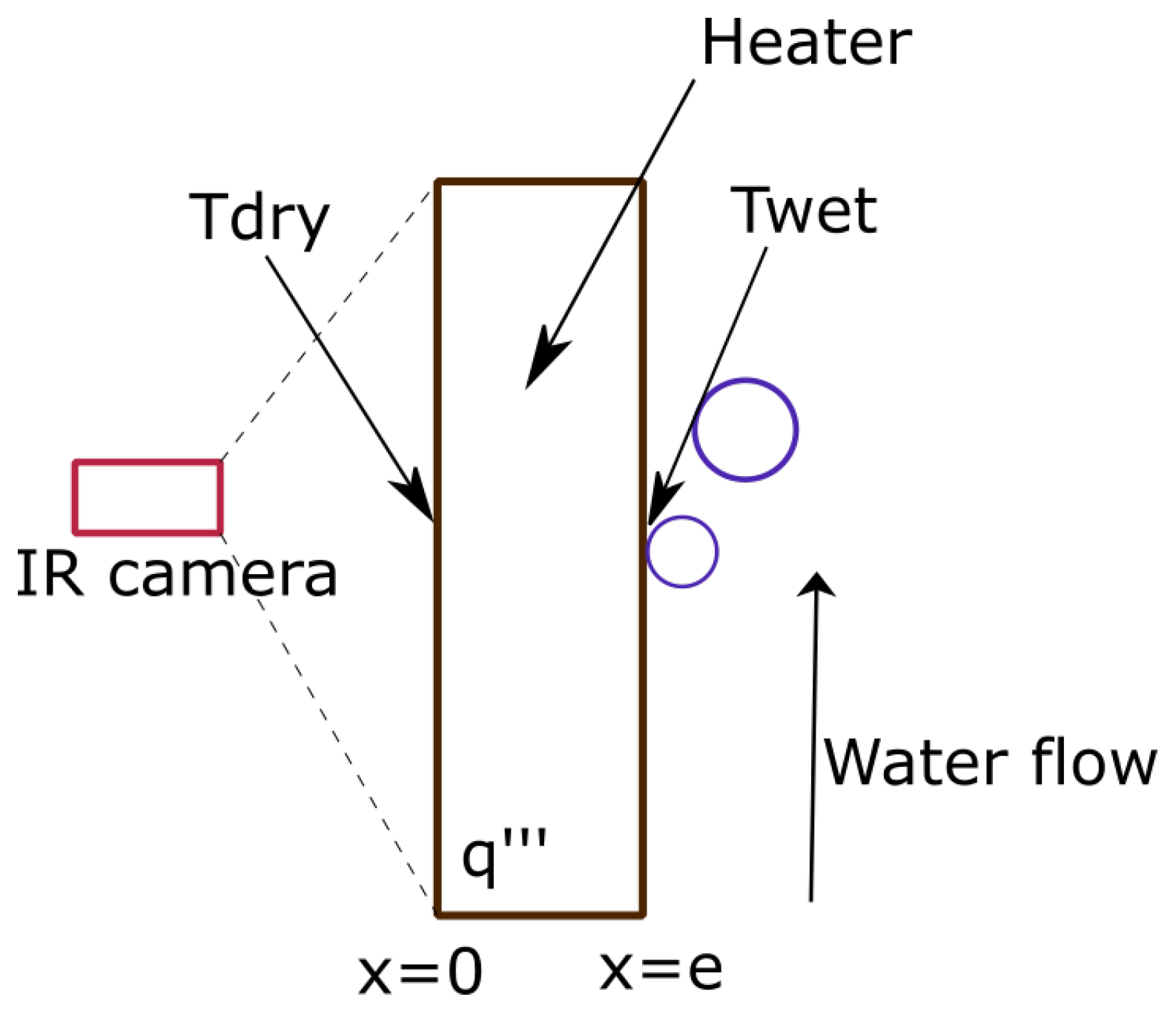
2. Experimental Setup

An experimental setup is currently being designed at CEA Cadarache. This setup involves a specific test section that will allow (i) a direct visualization of the boiling flow using the same technique as the one used by March [4] (shadowgraphy), but also (ii) a characterization of the temperature field from the wet side of the heated plate, similar to Richenderfer’s work [6].

Nevertheless, in order to account for the representativeness of the heating surface, we considered a metallic plate (stainless steel) instead of metallic coating as Richenderfer proposed [6], i.e., a plate whose thickness needs to be determined.

Figure 3 and Figure 4 depict a schematic of the future test section and its measurement systems.

Three sapphire windows will allow direct visualization of the bubbles created along the heated plate, which will be soldered on a fourth sapphire window to retain the fluid pressure. The metallic plate will be heated by the direct Joule effect.

The temperature of the heated plate will be measured on its external face (dry side $T_{dry}$) using an infra-red camera and the temperature of the wet side of the plate $T_{wet}$ will be deduced from the dry temperature by solving the heat diffusion equation within the plate (see Figure 5). The wet temperature may be useful to analyze the data collected by shadowgraphy through the sapphire windows. Indeed, as mentioned before, due to the thermal gradients in the vicinity of the heated wall ([4,8]), pictures obtained by shadowgraphy can be distorted, making the identification of the bubble detachment time, as a consequence the bubble lift-off diameter, difficult. It is believed that thermal imaging will be helpful as the bubble detachment should correspond to a local variation of the temperature field on the wet side of the heated plate. As an illustration, one can cite the recent work of Wang and Podowski [9], who calculated the temperature profile as a function of time under a nucleation site. Figure 6 describes the prototypical behavior of the wall temperature beneath a nucleation site as a function of time.

One can observe two distinct stages. First, while the bubble is still attached to its nucleation site and is growing, the temperature decreases because of the vaporization. Then, the bubble detaches from the heated wall at $t_g$ (called the growing time), and the temperature increases until a new bubble begins to grow on the nucleation site. $t_w$ is called the waiting time. Thermal imaging may help us to identify the time when the bubble effectively detaches from the wall ($t_g$).

Determining the plate thickness should then result in a compromise. On the one hand, the thickness should be large enough to ensure good representativeness of the heating surface and boiling; on the other hand, the thickness should be thin enough to allow for accurate determining of the temperature on the wet side of the heating plate. Figure 5 depicts the problem to be solved.

As a preliminary step, assuming that the plate thickness will be much lower than the other characteristic dimensions of the heater, a one-dimensional approach will be considered.

By solving the diffusion equation within the plate for a given set of boundary conditions, it is possible to determine the wet temperature $T_{wet}$. In the experimental configuration, all of the measurements will be performed on the external side. So the boundary conditions will be expressed on the same face (dry side of the plate). The associated heat conduction problem is then an inverse problem where the major characteristic is an ill-posed problem (from a mathematical point of view). As a consequence, the wet temperature, which is calculated by solving the diffusion equation, will be very sensitive to the boundary condition uncertainties (dry temperature and heat flux on this face).

3. Thermal Study of the Heater

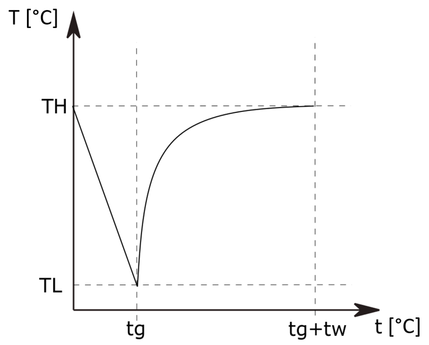
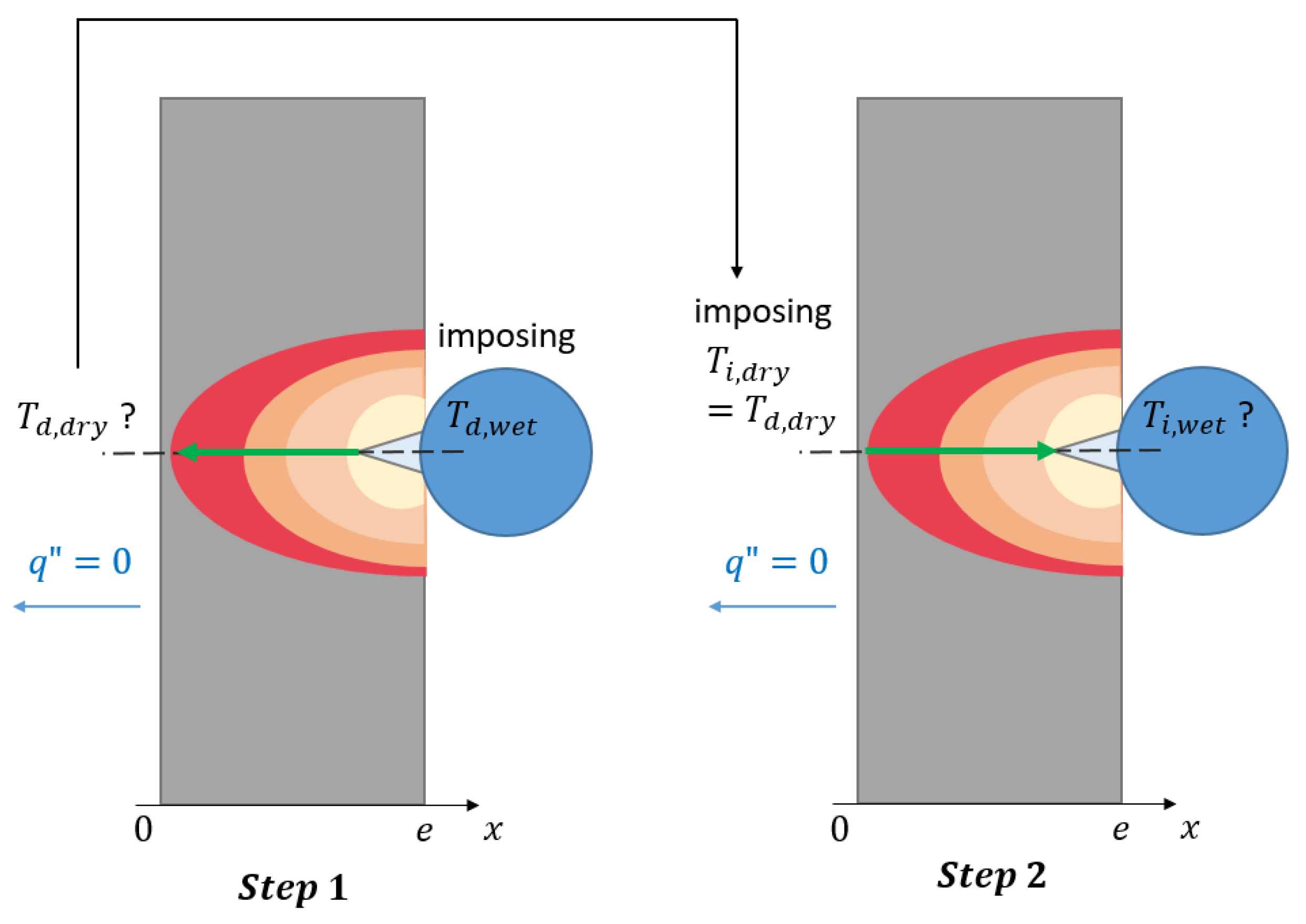
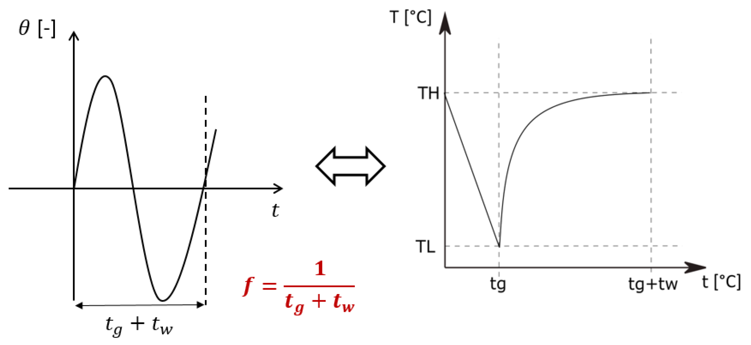
3.1. Methodology

To determine the thickness of the plate, a three-step methodology was implemented (see Figure 7).

(1)

In the first step, the direct heat conduction problem is solved within the plate for a given couple of boundary conditions expressed on both sides of the calculation domain:

(a)

On the dry side: $x=0$, $q^{″}=0$.

(b)

On the wet side: $x=e$, $T_{d,wet}=f\left(t\right)$.

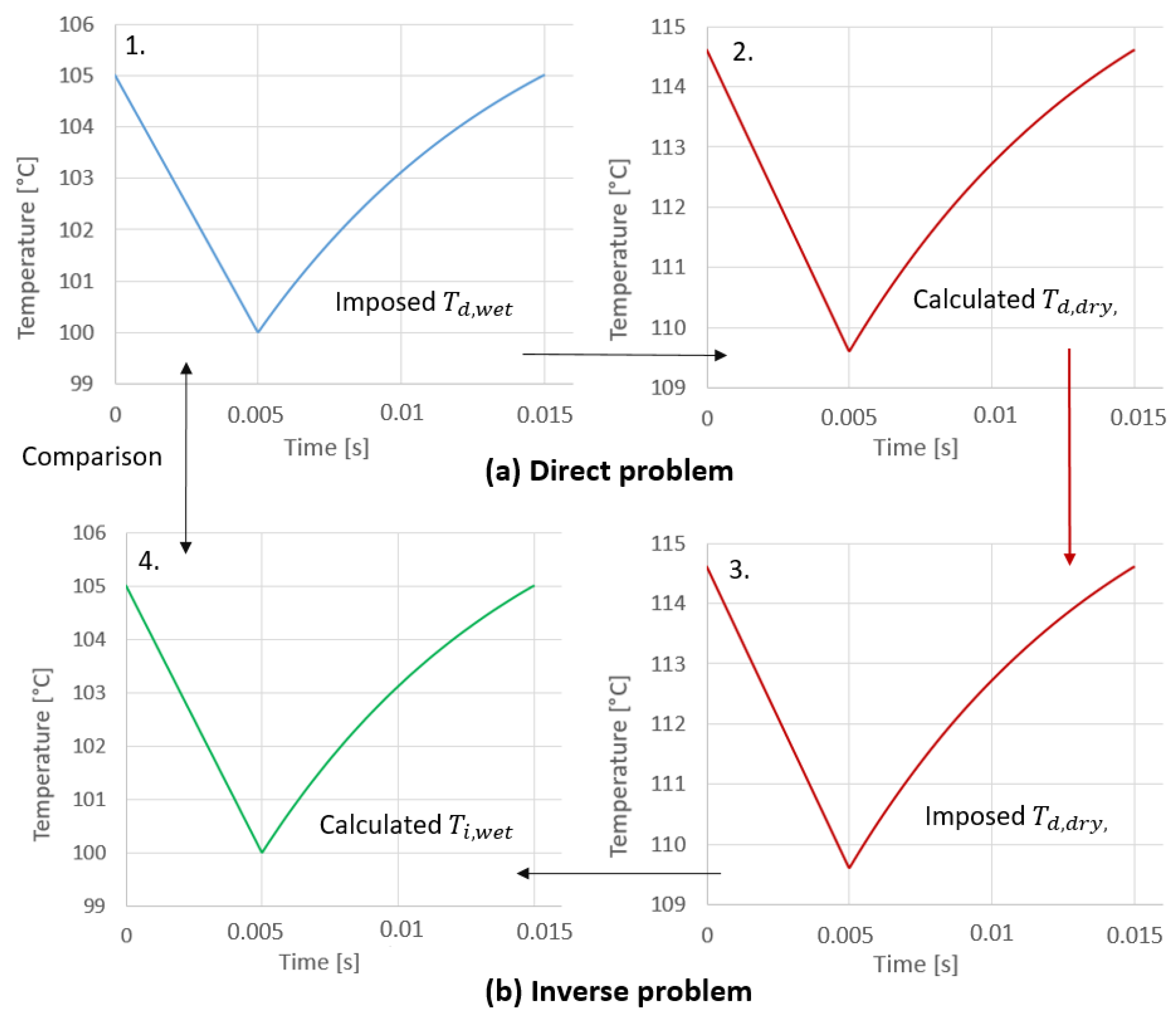
The objective is to calculate $T_{d,dry}=T(x=0,t)$ The subscript d indicates that the direct problem is being solved.

(2)

In the second step, the associated inverse heat conduction problem is studied by solving the diffusion equation for a given couple of boundary conditions expressed on the dry side of the plate:

(a)

On the dry side: $x=0$, $q^{″}=0$.

(b)

On the dry side: $x=0$, $T_{i,dry}(0,t)=T_{d,dry}(0,t)$.

The objective is to calculate the wet temperature $T_{i,wet}$ and to check whether $T_{i,wet}=T_{d,wet}$. The subscript i means that the inverse problem is being solved. One should notice that this configuration is very close to the one that will be encountered during the tests since $T_{d,dry}$ will effectively be measured by IR thermography.

(3)

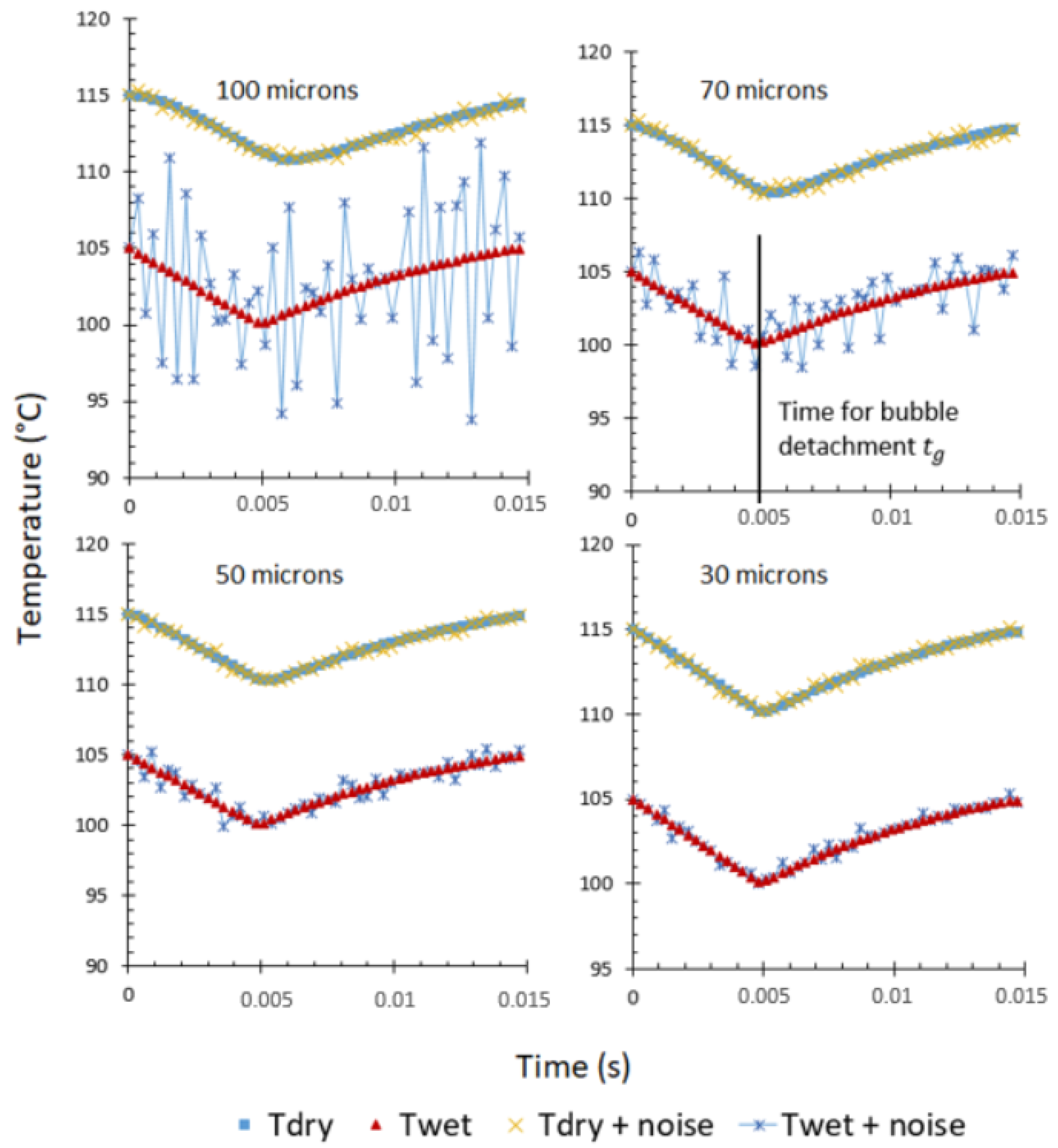
In the third step, a sensitivity analysis to the uncertainties of $T_{d,dry}$ will be performed.

3.2. Direct Problem

3.2.1. Modeling

The diffusion equation can be written as:

$$\begin{array}{|c|}\hline \rho C_P\frac{\partial T}{\partial t}=\lambda {\nabla }^{2}T+q^{‴}\\ \hline\end{array}$$

(1)

where $\rho$ is the density of the heater material, $C_P$ is the thermal capacity of the heater material, T is the temperature, t is time, $\lambda$ is the thermal conductivity of the heater material that is supposed to be constant, and $q^{‴}$ is the volumetric heat source due to the direct Joule effect. The power input is calculated as the product of the electrical resistance of the plate $R_{elec}$ and the squared intensity I. The intensity is imposed by an electrical power source in order to heat the plate through the direct Joule effect. For the rest of the study, the typical value for the current is $I=400$A. The volumetric heat source is then calculated using Equation (2).

$$q^{‴}=\frac{R_{elec}\ast I^2}{l\ast H\ast e}=\frac{{\rho }_{elec}\ast I^2}{l^2\ast e^2}$$

(2)

The time-dependent temperature profile on the wet side of the plate $T_{wet}$, described in Figure 6, is given by:

$$\begin{array}{|c|}\hline \begin{array}{cc}t<t_g& {\displaystyle T_{d,wet}(x=e)=\frac{T_L-T_H}{t_g}t+T_H}\\ t_g<t<t_g+t_w& {\displaystyle T_{d,wet}(x=e)=T_L+\frac{T_L-T_H}{1-e^{-1}}(1-e^{{\displaystyle \frac{t-t_g}{t_w}}})}\end{array}\\ \hline\end{array}$$

(3)

The initial condition is expressed as the solution to the steady problem:

$$\begin{array}{|c|}\hline \lambda {\nabla }^{2}T+q^{‴}=0\\ \hline\end{array}$$

(4)

$$\begin{array}{|c|}\hline \begin{array}{cc}\mathrm{Boundary} \mathrm{conditions}:\hfill & {\displaystyle \frac{\partial T}{\partial x}\left(x=0\right)=0}\\ \hfill & T\left(x=e\right)=T_H\end{array}\\ \hline\end{array}$$

(5)

3.2.2. Preliminary Magnitude through Analytical Analysis

To determine the first order of magnitude of the thickness, a simple analytical analysis was carried out. The attenuation and phase shift properties of a metal plate subjected to a variable temperature field as a boundary condition were to be estimated in a simple configuration. By considering a harmonic variation, one can analytically determine this behavior and identify the skin thickness at which the thermal information can no longer be identified.

As the first approach, a harmonic time-dependent temperature was applied on the boundary of a semi-infinite wall (see Figure 8) with the following thermal Equations (6)–(9).

$$\begin{array}{|c|}\hline \rho C_P\frac{\partial \theta }{\partial t}=\lambda \frac{{\partial }^2\theta }{\partial x^2}\\ \hline\end{array}$$

(6)

with $\theta =T-T_0$, T the temperature, $T_0$ the initial temperature.

The boundary condition at $x=0$, ${\theta }_{wall}$, is defined as:

$$\begin{array}{|c|}\hline {\theta }_{wall}(x=0,t)={\theta }_{0}cos\left(\omega t\right)\\ \hline\end{array}$$

(7)

where $\omega =2\pi f$ and f the frequency.

The boundary condition for an infinite wall is defined as:

$${\theta }_{\infty }(x=\infty ,t)=0$$

(8)

The initial condition ${\theta }_{initial}$ is:

$${\theta }_{initial}(x,t=0)=0$$

(9)

The solution of Equations (6)–(9) can be written as:

$$\theta (x,t)=e^{i\omega t}f\left(x\right)$$

(10)

Using the boundary and initial conditions, the solution $\theta$ can be expressed as:

$$\begin{array}{|c|}\hline \theta (x,t)={\theta }_0{e}^{\sqrt{\frac{\omega }{2\alpha }}x}cos\left(\omega t-\sqrt{\frac{\omega }{2\alpha }}x\right)\\ \hline\end{array}$$

(11)

where $\alpha$ is the thermal diffusivity.

With this simple expression, the temperature attenuation within the plate can be calculated. The signal frequency is deduced from time $t_g$ and $t_w$, characterizing the temperature variation under a nucleation site (see Figure 9).

The plate will be made of INOX 316L, whose thermal diffusivity is $\alpha$ = 3.75 × 10${}^{-6}$ m${}^2$·s${}^{-1}$ (assumed to be constant). According to Unal [3], the following orders of magnitude for $t_g$ and $t_w$ can be considered:

$$t_g\approx 5\times {10}^{-3}\mathrm{s}\mathrm{and}{t}_w\approx 1\times {10}^{-2}\mathrm{s}$$

(12)

Calculation details are presented in Appendix A. The frequency of the temperature variation is then equal to 60 Hz.

Figure 10 shows the evolution of the bandwidth (blue curve) and time delay (red curve) within the plate as a function of the thickness. It indicates that after 100 µm (green vertical limit) the information is not correctly detectable according to the blue curve: an attenuation by a factor of 2 is noted. This is the first limit that can be fixed for the thickness of the plate. Moreover, the time delay is almost 0.75 s for a 100 µm thickness.

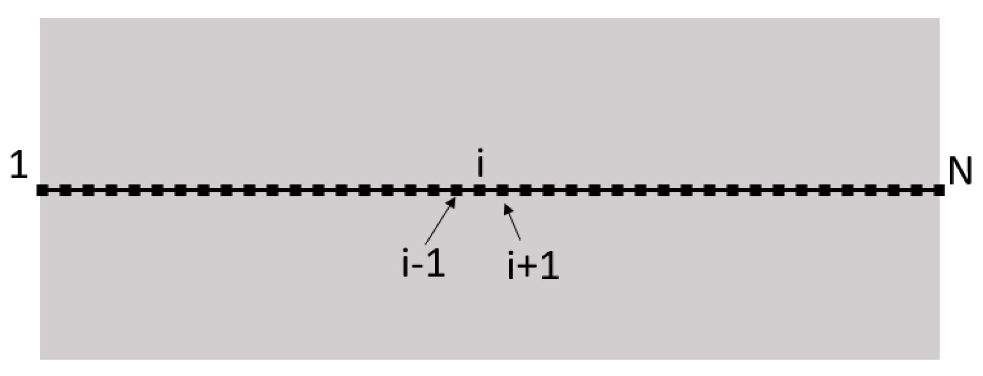
3.2.3. 1D Solving

The diffusion Equation (1) can be written in 1D as:

$$\begin{array}{|c|}\hline \rho C_P\frac{\partial T}{\partial t}=\lambda \frac{{\partial }^{2}T}{\partial x^2}+q^{‴}\\ \hline\end{array}$$

(13)

$$\begin{array}{|c|}\hline \begin{array}{cc}\mathrm{Boundary} \mathrm{conditions}:\hfill & {\displaystyle \frac{\partial T}{\partial x}\left(0,t\right)=0}\\ \hfill & T\left(e,t\right)=T_{d,wet}\left(t\right)\end{array}\\ \hline\end{array}$$

(14)

$$\begin{array}{|c|}\hline \begin{array}{cc}\mathrm{Initial} \mathrm{condition}:\hfill & T\left(x,0\right)=T_{d,initial}\left(x\right)\end{array}\\ \hline\end{array}$$

(15)

where $T_{d,initial}\left(x\right)$ is the solution of the steady-state problem defined by Equations (4) and (5) expressed in Equation (16).

$$T_{d,initial}=\frac{q^{‴}}{2\lambda }(x^2-e^2)+T_H$$

(16)

The steady-state problem–solution expressed in Equation (16) is a parabolic profile as shown in Figure 11 as it is a one-dimensional problem.

Equations (13)–(15) are solved by finite differences using a second-order-centered scheme for the Laplacian and an implicit scheme for time dependence. The temperature $T\left(0,t\right)$ is then calculated. This temperature will be noticed $T_{dry}$.

After meshing the plate with a regular mesh size along the axis (see Figure 12), Equations (13)–(15) are solved by finite differences using a second-order centered scheme for the Laplacian (17) and an implicit scheme for time dependence (18).

$$\begin{array}{cc}\mathrm{for}2<i<N-1& \frac{{\partial }^{2}T}{\partial x^2}=\frac{T_{i+1}-2T_i+T_{i-1}}{\mathsf{\Delta }{x}^2}\\ \mathrm{for}i=1& \frac{{\partial }^{2}T}{\partial x^2}=\frac{T_2-T_1}{\mathsf{\Delta }{x}^2}\\ \mathrm{for}i=N& T_N=T_{d,wet}\end{array}$$

(17)

$$\begin{array}{cc}\mathrm{for}1<i<N& {\left(\frac{\partial T}{\partial t}\right)}^{n+1}=\frac{T_i^{n+1}-T_i^n}{\mathsf{\Delta }t}\end{array}$$

(18)

At the preliminary stage, the implemented numerical model was validated. Spatial and temporal mesh sensitivity studies were performed to check convergence. The configurations tested in the following result from these sensitivity studies. These studies show that convergence was reached for $N=50$ and $n=50$.

On the other hand, the computational tool was validated by comparing the results for several configurations (with simple boundary conditions) whose documented analytical solutions are available in the literature [10].

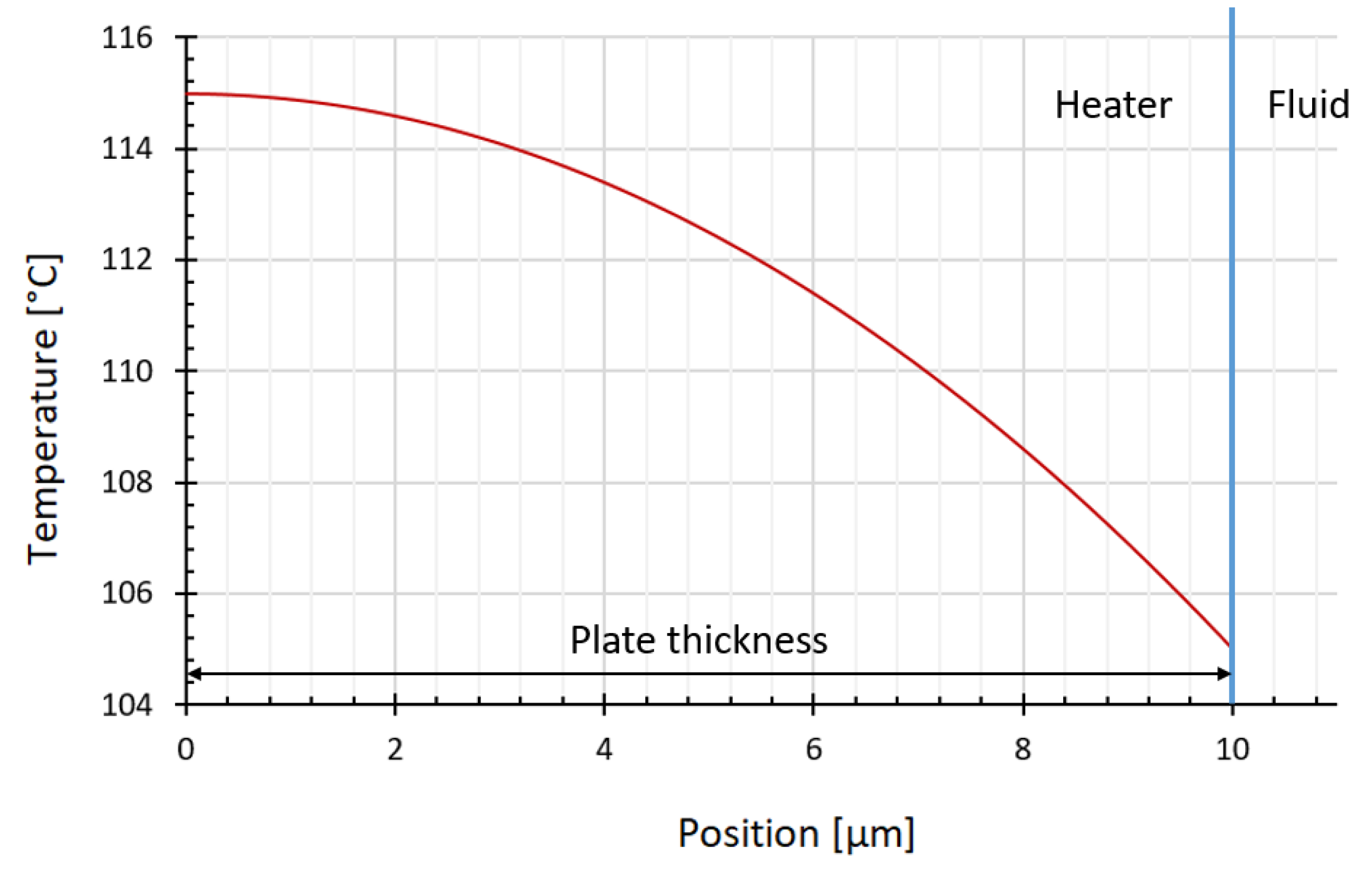
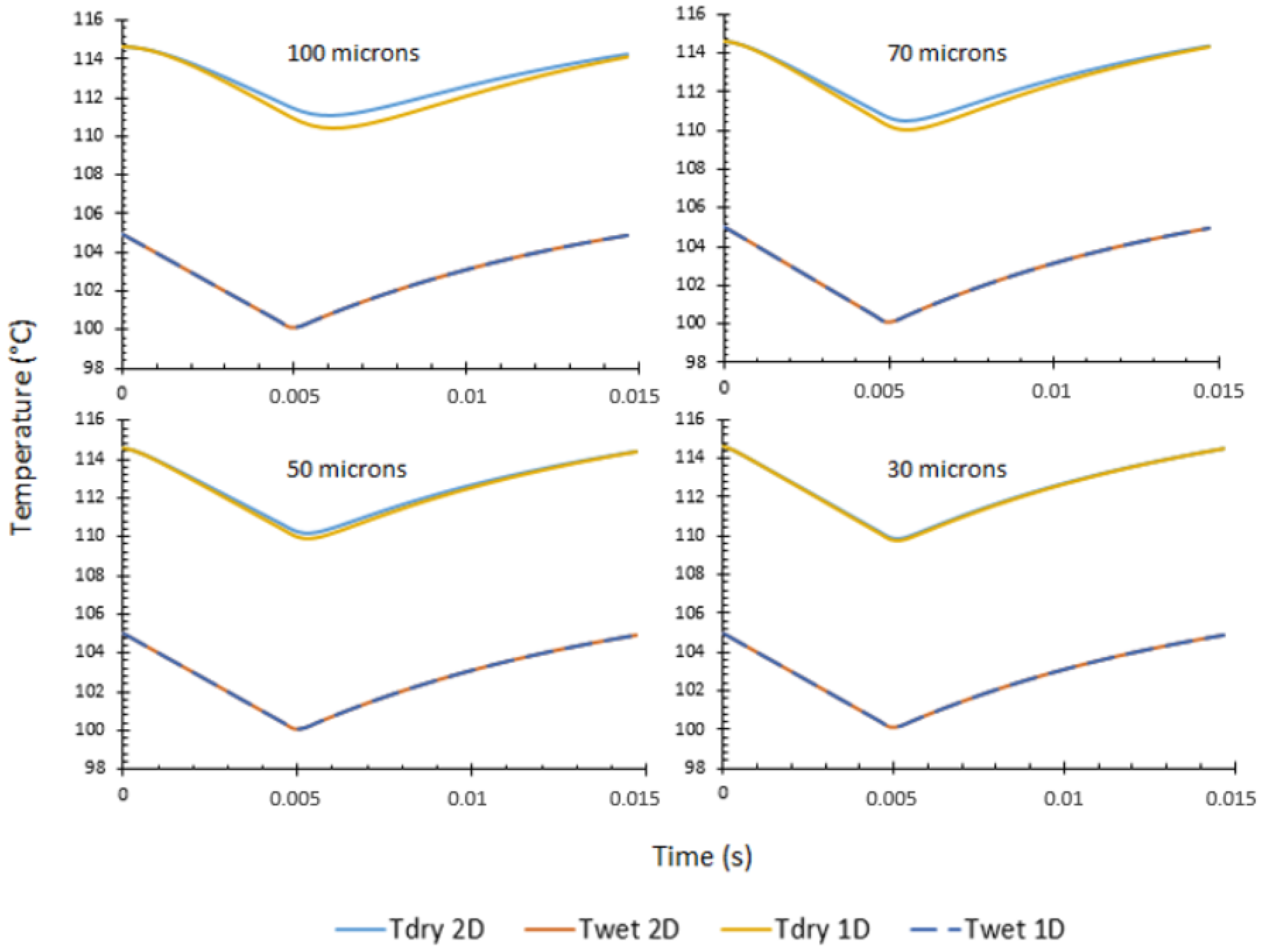
3.2.4. Thickness Calculation

The direct 1D model leads to the first result for the plate thickness.

Figure 13 displays the variation in the temperature on the dry side of the plate for the previous time-depending boundary condition (Section 3.2.3) as a function of the plate thickness (ranging from the 1 µm blue curve to the 500 µm orange curve). It appears that for thicknesses higher than the 100 µm yellow curve, the calculated dry temperature strongly differs from the wet temperature.

The right figure of Figure 13 points out the time phase shift for a thickness ranging from a 10 µm green curve to a 100 µm yellow curve. For a thickness equal to 100 µm, the phase shift represents almost 20% of the time scale that we aim to measure, which implies that this thickness cannot be exceeded. The temperature variation of 5 ${}^{\circ }$C initially imposed on the wet side results in a variation of 4.2 ${}^{\circ }$C on the dry side of the plate of 100 µm thickness.

This result is in accordance with the preliminary study of the order of magnitude in Section 3.2.2, and confirms that the thickness should not exceed 100 µm.

3.3. Inverse Problem

3.3.1. Measurement Techniques

As explained in Section 2, the temperature of the heated plate will be measured on its external face (dry side, $T_{dry}$) using an infra-red camera and the temperature of the wet side of the plate ($T_{wet}$) will be deduced from the dry temperature by solving the heat diffusion equation within the plate.

The purpose here is to determine if the measurement of the dry temperature will make it possible to deduce the wet temperature with an acceptable uncertainty.

Since boundary conditions are imposed on a single face of the plate (dry side), the heat conduction within the plate is called an inverse problem; such problems are ill-posed according to Hadamard [11]. This implies that the solution to this problem is very sensitive to potential uncertainties in the boundary conditions. The following section is then dedicated to the study of this key point.

3.3.2. Methodology

In Section 3.2.3, we imposed the wet temperature variation and determined the corresponding dry temperature from it. The idea here is (i) to check whether, in the context of the inverse problem, it is possible to reconstruct the wet temperature $T_{wet}$ that had been imposed from the dry temperature calculated previously $T_{d,dry}$, and (ii) to check the impact of an uncertainty (or measurement noise) on $T_{dry}$ and the construction of the wet temperature $T_{wet}$. This study will be performed using the 1D approach. The inverse problem is, therefore, characterized by the solution of the following system:

$$\begin{array}{|c|}\hline \rho C_P\frac{\partial T}{\partial t}=\lambda \frac{{\partial }^{2}T}{\partial x^2}+q^{‴}\\ \hline\end{array}$$

(19)

$$\begin{array}{|c|}\hline \begin{array}{cc}\mathrm{Boundary} \mathrm{conditions}:\hfill & {\displaystyle \frac{\partial T_i}{\partial x}\left(0,t\right)=0}\\ \hfill & T_i\left(0,t\right)=T_{d,dry}\left(t\right)\end{array}\\ \hline\end{array}$$

(20)

The dry temperature is taken as the result of the direct 1D problem Section 3.2.3.

The initial condition is given by:

$$T\left(x,0\right)=T_{i,initial}\left(x\right)$$

(21)

where $T_{i,initial}\left(x\right)$ is the solution of the steady-state problem:

$$\begin{array}{|c|}\hline \begin{array}{cc}\mathrm{Problem} \mathrm{equation}:\hfill & {\displaystyle \lambda \frac{{\partial }^2{T}_i}{\partial x^2}=-q^{‴}}\\ \mathrm{Boundary} \mathrm{conditions}:\hfill & {\displaystyle \frac{\partial T_i}{\partial x}\left(0\right)=0}\\ \hfill & T_i\left(0\right)=T_{d,dry}\left(0,0\right)\end{array}\\ \hline\end{array}$$

(22)

The temperature $T\left(e,t\right)$ is then calculated by solving the heat conduction equation with conditions described from Equations (20)–(22). This temperature is noticed $T_{i,wet}$ and will be compared to $T_{d,wet}\left(t\right)$.

3.3.3. Results

The inverse problem was solved with finite differences (similar to the direct problem). Figure 14 shows the steps to solve the inverse problem. The direct problem was solved by imposing a temperature variation over the wet side of the plate (internal face) $T_{d,wet}$. The solution is the temperature variation on the external face of the plate $T_{d,dry}$. The inverse problem is then solved by imposing on the external face the temperature as $T_{d,dry}$, resulting from the direct problem calculation. The solution to the inverse problem is the temperature on the internal face $T_{i,wet}$, which can be compared with the one imposed first $T_{d,wet}$.

Figure 14 shows that the inverse solution for the wet temperature is valid: the exact same wet temperature imposed at the beginning for any parameter is calculated (blue and green curves).

As with all inverse problems, it is sensitive to boundary condition uncertainties. A random uncertainty (white noise) of ±0.5 ${}^{\circ }$C is then applied to the measurement on the outside (dry temperature).

Imposing this uncertainty to the dry-side temperature $T_d(0,t)$, one can observe (as a consequence) amplification of the noise for the wet temperature $T_{i,wet}$.

Figure 15 shows the influence of the plate thickness on the accuracy of the calculated wet temperature. The blue and red triangles are the initial results for the dry and wet temperatures (without any uncertainties). The yellow crosses correspond to the dry temperature taking into account the uncertainty. The blue crosses are the results of the inverse problem with the noisy dry calculated temperature. For a thickness of 100 µm, the amplification leads to the impossibility of finding the time scales that are to be measured, especially the bubble time detachment. Decreasing the thickness leads to decreasing the noise on the reconstructed wet temperature.

A 70 µm thickness enables detecting the change of slope and, therefore, the time of detachment of the bubble, which makes it possible to measure the frequency of bubble detachment from the wall. However, the apparent noise shows an oscillation of 5 ${}^{\circ }$C around the actual temperature value. For the study of boiling that is envisaged on the future device, a more accurate temperature measurement may be of interest. Indeed, the classical wall-superheat models indicate that a few degrees of variation are expected for the given set of conditions, and the noise of the measurements restricted to 1 or 2 ${}^{\circ }$C will make it easier to identify the temperature to be compared with the models.

The 50 µm seems to be a good thickness for the plate. The noise is reduced, the identification of the quantity of interest (in time and temperature) is a more accurate (2 ${}^{\circ }$C) variation around the actual temperature value). As a consequence, 50 µm is then the new upper limit for the plate thickness.

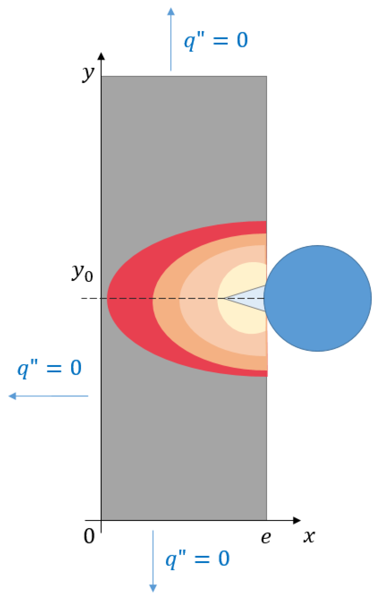
4. Spatial Resolution of the Measurements

In this Section, the aim is to determine the spatial resolution of the measurement by using a 2D model for this problem. This 2D study should confirm the 1D approach developed above. The 1D approach was given for bubble diameters that are an order of magnitude larger than the plate thickness studied: $D\gg e$. It is important to verify the behavior of the plate with a bubble whose diameter is of the order of the thickness of the plate: $D\approx e$. The 2D effects in this problem are inherent to the fact that the plate is powered by the direct Joule effect and, therefore, with an internal heat source. The resistance of the plate drives the flux distribution and any change in temperature impacts this distribution and can create inhomogeneities or oppose a temperature change. First, the 2D model is presented with a comparison between the 2D and 1D results for a large bubble ($D\gg e$). Then a sensitivity study is carried out to establish the thickness at which a bubble of a fixed size (pressure dependent) can be detected by an IR camera on the dry side (in the case of $D\approx e$). Finally, we are interested in the minimum distance between two bubbles for them to be detected independently of each other by an IR camera on the dry side of the plate.

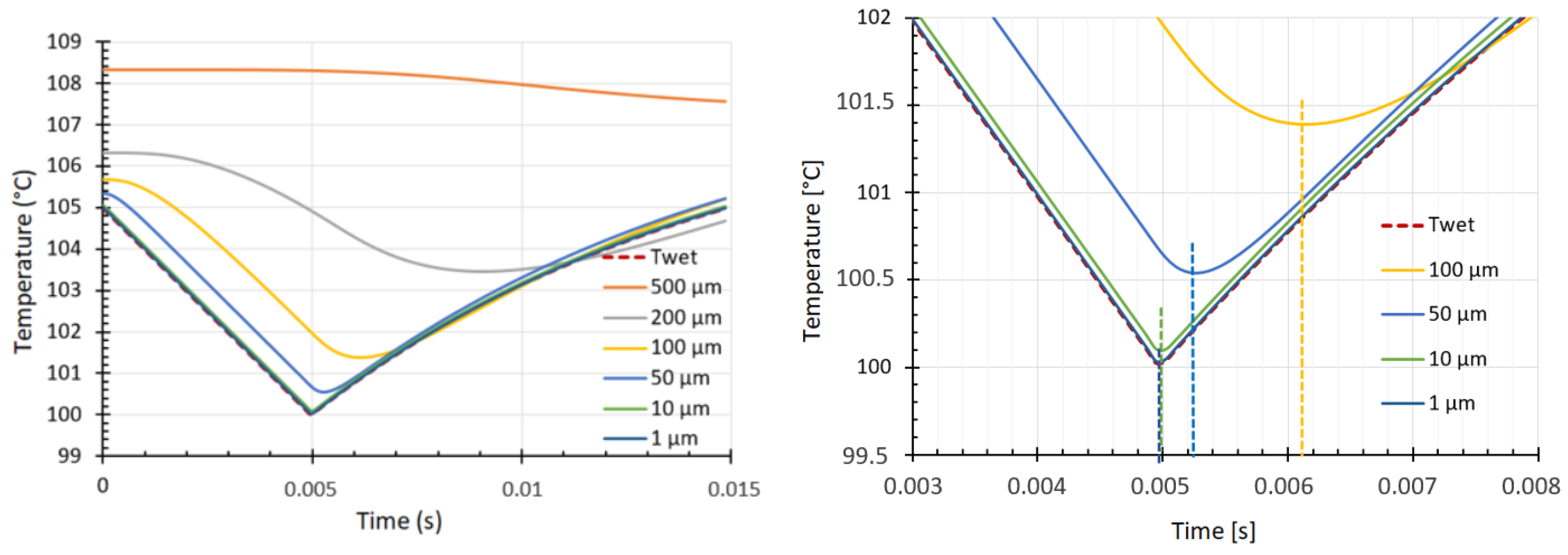
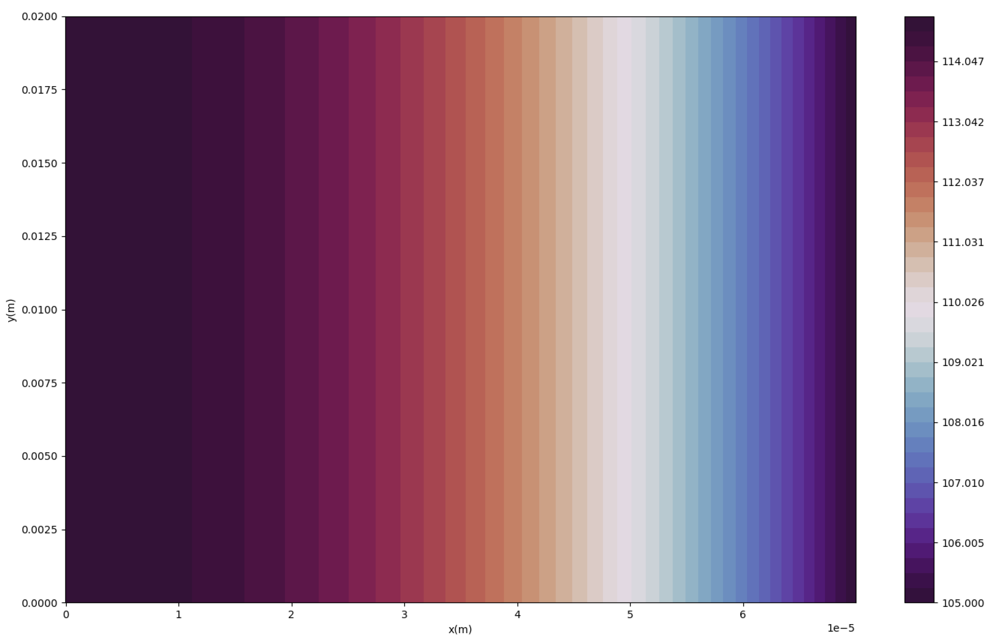
4.1. 2D Diffusion Influence

In order to assess the validity of a 1D approach, some calculations using a 2D description of the heater were performed.

The general diffusion Equation (1) can be written for a 2D approach as:

$$\begin{array}{|c|}\hline \rho C_P\frac{\partial T}{\partial t}=\lambda (\frac{{\partial }^{2}T}{\partial x^2}+\frac{{\partial }^{2}T}{\partial y^2})+q^{‴}\\ \hline\end{array}$$

(23)

where x and y are the space variables.

The boundary conditions are:

$$\begin{array}{|c|}\hline \begin{array}{cc}\mathrm{Boundary} \mathrm{conditions}:\hfill & {\displaystyle \frac{\partial T}{\partial x}\left(0,y,t\right)=0}\\ \hfill & T\left(e,y,t\right)=T_{d,wet}\left(y,t\right)\\ \hfill & {\displaystyle \frac{\partial T}{\partial y}\left(x,0,t\right)=0}\\ \hfill & {\displaystyle \frac{\partial T}{\partial y}\left(x,l,t\right)=0}\end{array}\\ \hline\end{array}$$

(24)

The temperature on the wet side of the plate $T_{wet}$ is given by:

$$\begin{array}{|c|}\hline \begin{array}{cc}\mathrm{for}t<t_g \mathrm{and} y=y_0& {\displaystyle T_{d,wet}(x=e,y=y_0)=\frac{T_L-T_H}{t_g}t+T_H}\\ \mathrm{for}{t}_g<t<t_g+t_w \mathrm{and} y=y_0& {\displaystyle T_{d,wet}(x=e,y=y_0)=T_L+\frac{T_L-T_H}{1-e^{-1}}(1-e^{{\displaystyle \frac{t-t_g}{t_w}}})}\\ \forall t \mathrm{and} y\ne y_0& T_{d,wet}=T_H\end{array}\\ \hline\end{array}$$

(25)

where $y_0$ is the position of a nucleation site on the plate (see Figure 16).

The initial condition is:

$$T\left(x,y,0\right)=T_{d,initial}\left(x,y\right)$$

(26)

where $T_{d,initial}\left(x,y\right)$ is the solution of the steady-state problem where the boundary conditions are ($T_H$ is the same as defined in Figure 6):

$$\begin{array}{|c|}\hline \begin{array}{cc}\mathrm{Problem} \mathrm{equation}:\hfill & {\displaystyle \lambda (\frac{{\partial }^{2}T}{\partial x^2}+\frac{{\partial }^{2}T}{\partial y^2})=-q^{‴}}\\ \mathrm{Boundary} \mathrm{conditions}:\hfill & {\displaystyle \frac{\partial T}{\partial x}\left(0,y\right)=0}\\ \hfill & T\left(e,y\right)=T_H\\ \hfill & {\displaystyle \frac{\partial T}{\partial y}\left(x,0\right)=0}\\ \hfill & {\displaystyle \frac{\partial T}{\partial y}\left(x,l\right)=0}\end{array}\\ \hline\end{array}$$

(27)

The 2D steady-state temperature distribution is presented in Figure 17.

Equations (23)–(27) are solved by finite differences using a second-order central scheme for the Laplacian and an implicit scheme for time dependence. The temperature $T\left(0,t\right)$ is then calculated. This temperature is noticed $T_{dry}$.

Figure 18 displays, for different thicknesses, the influence of the 2D effects on the temperature beneath the nucleation site at $y=y_0$. This figure aims to point out the diffusion effect between 1D and 2D models. The yellow curves are the 1D direct result of the conduction within the plate, whereas the blue curve depicts the 2D direct calculations of this conduction problem. It shows that the gap between 1D and 2D simulations is decreasing with the thickness: from a maximum gap of 0.21 ${}^{\circ }$C at 100 µm to 0.07 ${}^{\circ }$C at 50 µm. This gap will not affect the 1D conclusion over the limit thickness. The 1D modeling is then sufficient to raise a first assessment of the plate geometry, as long as the bubble size is not smaller than the thickness of the plate.

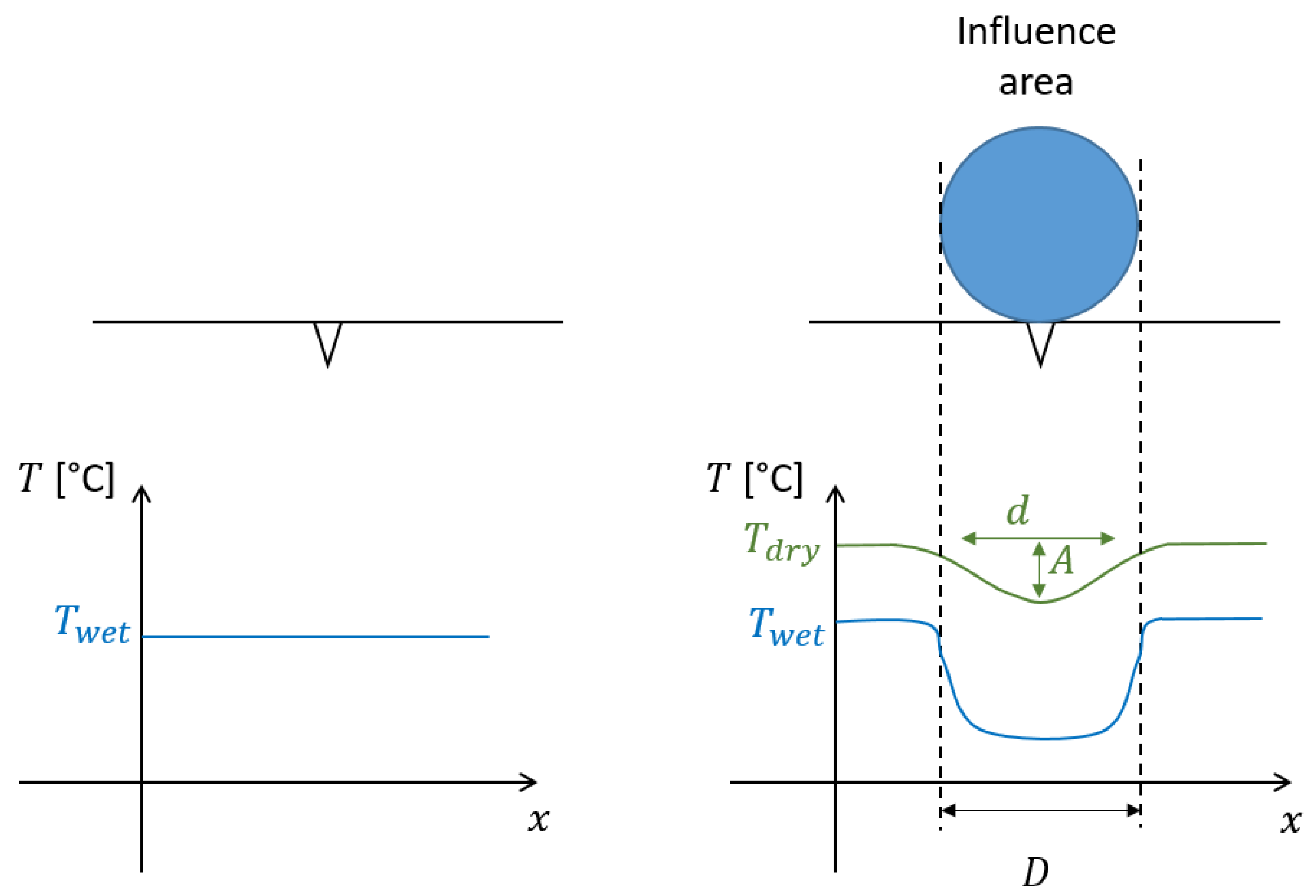
4.2. Thermal Influence Area of a Bubble Growth

When a bubble grows at a nucleation site, a temperature variation results under the bubble. Figure 19 shows the area of influence of a bubble on the wall temperature. When there is no bubble, the temperature is constant (right side), when a bubble grows on the wall (left side), the temperature variation studied in 1D appears on a zone, defined here as being the bubble diameter. The temperature variation on the dry side then appears to be attenuated in amplitude, and the influence area is expanded because of 2D diffusion effects. It is important to check that this temperature variation is measurable in two steps: (i) check that the amplitude A of this variation is measurable and, therefore, larger than the resolution of the camera (its ability to detect a temperature variation), (ii) check that the size of the spot d is larger than a camera pixel, to be able to detect it.

Let us recall that the aim of these measurements is to detect the timescales of the bubble growth on the plate from low to high-pressure conditions. Unal’s correlation [3] gives an order of magnitude of the bubble diameter as a function of the thermal-hydraulic conditions. For our prototypical conditions, the bubble diameter ranges from 40 µm to 800 µm for pressure from 110 to $1$bar, respectively.

For each of these conditions (pressure, bubble size), the maximum thickness over which the bubble cannot be detected by IR measurements has to be determined.

The IR camera generally presents a theoretical temperature resolution of 50 mK (a good calibration must be carried out beforehand). As the first criterion, we will consider that a variation of the wall temperature (dry side) of 1 ${}^{\circ }$C is enough to detect a bubble attached to the wall. In order to consider bubble timescales to be measurable, a second criterion was set. The detachment of the bubble will induce a slightly higher temperature variation so that a second step corresponding to a variation of 2 ${}^{\circ }$C of the wall temperature is considered. Moreover, conventional detectors for high-speed, high-performance cameras have pixel sizes in the range of 10 to 25 µm. The bubble detection criterion for the size of the influence area d is, therefore, set at 2 pixels or 50 µm.

As an example, Figure 20 shows (for a bubble size corresponding to 120 µm for a pressure of $P=50$bar and a temperature variation of 5 ${}^{\circ }$C under the nucleation site) the limit thickness selection, with the red-dashed curve named the 1 ${}^{\circ }$C limit for the detected first criterion and the blue-dashed curve named the 2 ${}^{\circ }$C limit for the measurement of the second criterion.

The determination of the thickness is done in two steps:

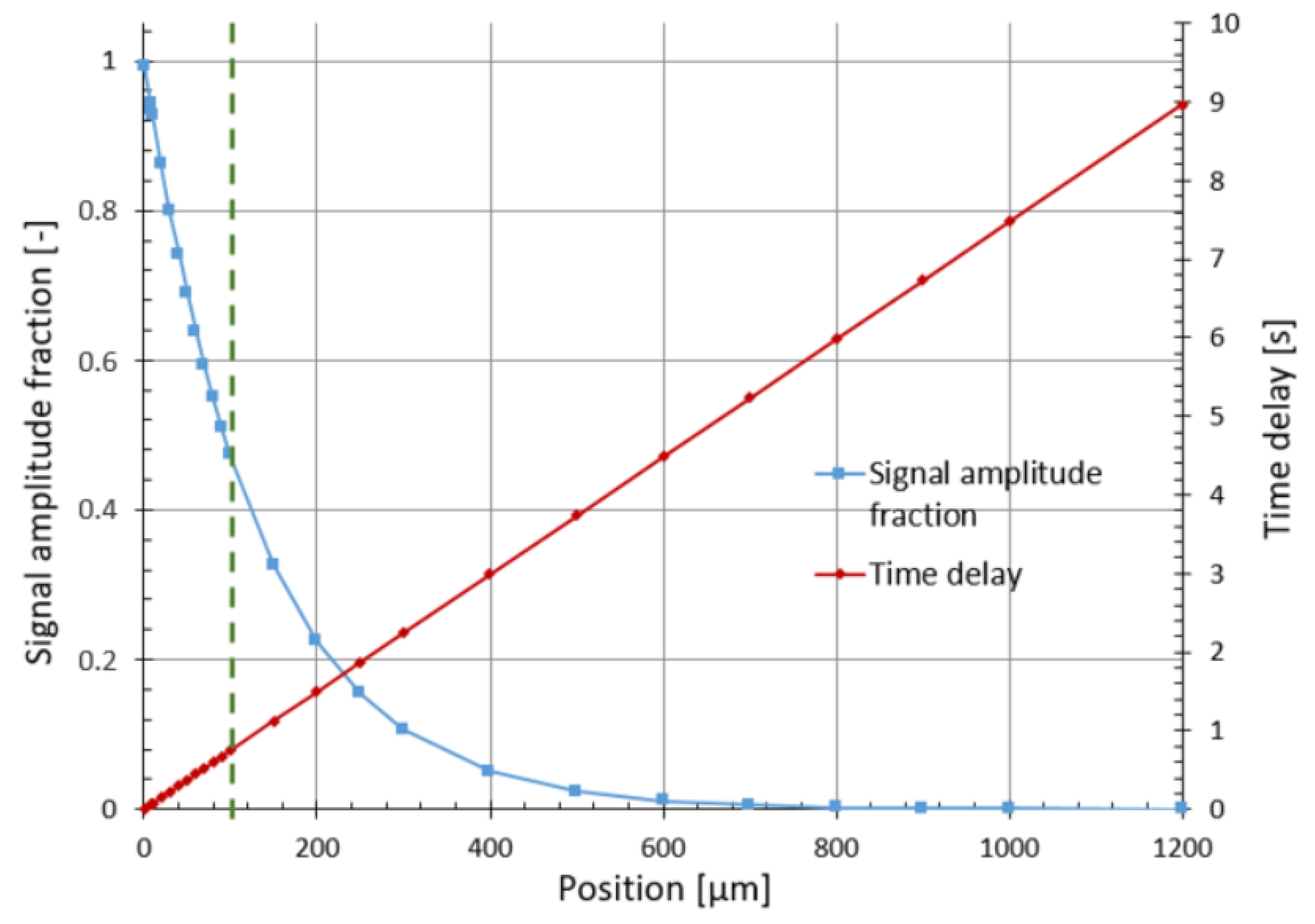
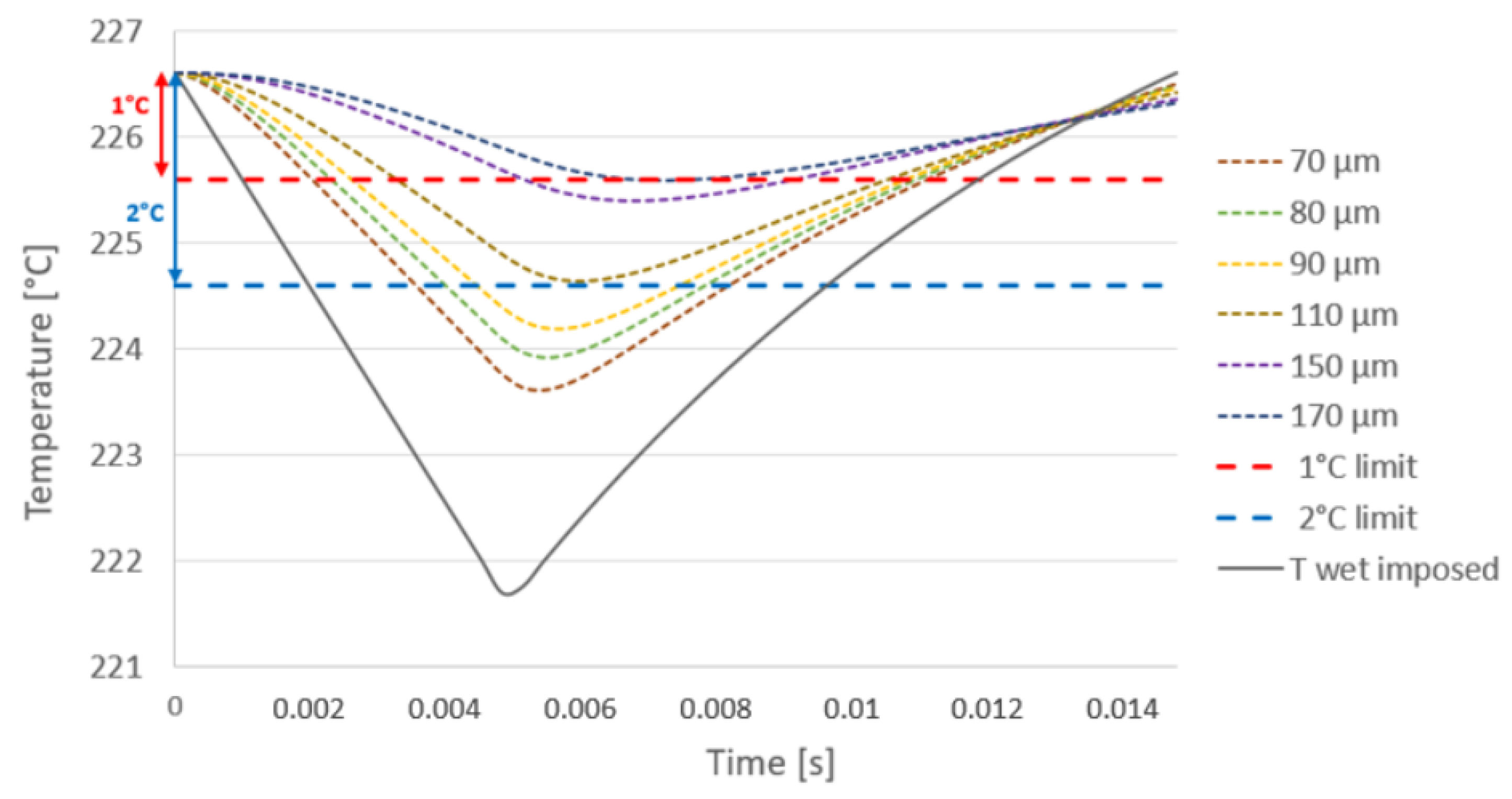
• The first step consists of identifying the thickness corresponding to the camera-readable amplitude of the dry-side temperature variation (example Figure 20; criteria 1 gives a 170 µm of thickness, criteria 2 gives 110 µm of thickness.),
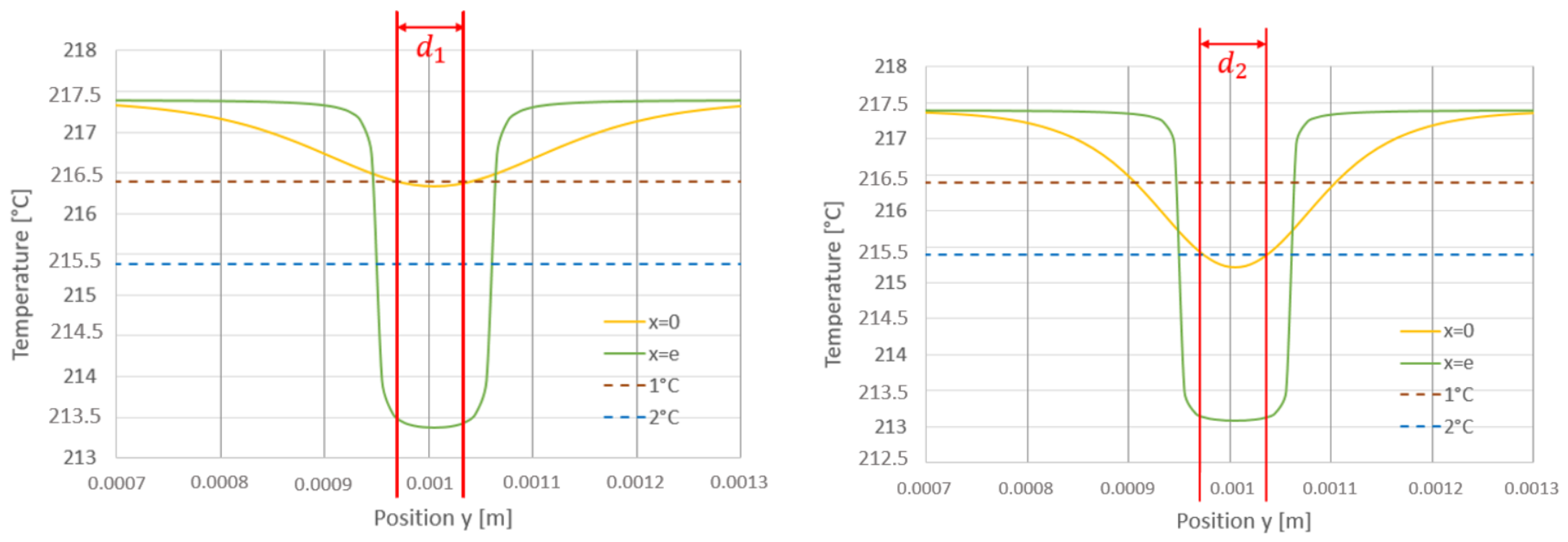
• The second step determines the dry-side influence area considering the two temperature criteria (see Figure 21; criteria 1’s thickness is valid ($d_1$ = 60 µm), but criteria 2 correlates with 100 µm of thickness ($d_2$ = 60 µm)).

Table 1. Spatial resolution: thickness range associated with the bubble size (pressure dependent).

Bubble Size µm	Pressure bar	First Criterion: Detection Thickness µm	Second Criterion: Measurement Thickness µm
800	1	250	200
120	20	170	110
70	50	100	60
50	80	70	40
40	110	65	35

summarizes (for the pressure and bubble size) the thickness corresponding to the first and second sets of criteria defined above. These values were identified after the two steps of checking the amplitude and area of influence explained before.

This result shows that a 50 µm thickness is a good compromise to be able to detect bubbles over the plate, to measure the timescales of the bubble growth and to maintain a sufficient thickness to ensure the representativeness of the surface. For higher pressure values, the bubble size calculated with the Unal correlation [3] decreases, and the temperature variation under this bubble could be more complicated to capture.

4.3. Discretization between Two Bubbles Growing on the Plate

With the same 2D model, the space meshing between two bubbles (depending on the thickness of the plate) is also checked, as shown in Figure 22. For a fixed thickness, the space between two bubbles of the same size increases until they can be detected independently from each other on the dry side of the plate (see Figure 22).

Table 2. Meshing of the method.

Thickness	Bubble Size	Minimum Gap for Detection
µm	µm	µm
70	200	60
70	50	120
50	200	40
50	50	100
30	200	20
30	50	60

summarizes the minimum gap between two bubbles to be detected independently (and not seen as one). The thickness of 50 µm will provide a discretization of 40 µm for bubbles with a diameter of 200 µm and 100 µm for bubbles with a diameter of 50 µm.

5. Conclusions

A setup is currently being designed at CEA Cadarache to provide characteristic measurements of nucleate boiling in forced convection for PWR’s prototypical conditions. This device will involve a heated plate whose internal face will be in contact with the coolant fluid (pressurized water), whereas temperature measurements will be carried out on its external face using IR thermography. The aim of this study was to define the geometry of the heating plate, allowing such measurements. The focus of this work was on the heater thickness, which is believed to be the most influential parameter.

A study of the thermal behavior of the plate was presented. First of all, the study of the conduction in the plate allows fixing a maximum limit for the plate thickness. This first limit was set at 100 microns. As the measurements are made on the external face of the plate, it will be necessary to reconstruct the wet temperature from these measurements by solving the inverse conduction heat transfer problem through the heated plate. in solving the inverse problem, a second limit over the thickness of the plate is fixed. This limit aims to minimize the amplification of uncertainties due to the inverse character of this problem. This second limit is set at 50 microns.

In the third step, a study was presented to determine the spatial resolution of this method. Through a 2D approach, for every range of pressure, the thickness to detect the associated bubble size was selected. In addition, the minimum discernible gap between two bubbles was determined. To enhance this result, more realistic boundary conditions could be imposed and should confirm the choice for the thickness of 50 microns.

The future test section will allow optical access to the flow and infrared measurements. The direct Joule’s heating plate will have a thickness determined by this study at 50 microns.

References

- Kurul, N.; Podowski, M. Multidimensional effects in forced convetion subcooled boiling. In Proceeding of the 9th International heat Transfer Conference, Jerusalem, Israel, 19–24 August 1990. [Google Scholar]
- Cole, R. Bubble frequencies and departure volumes at Subatmospheric Pressures. AIChe J. 1966, 13, 779–783. [Google Scholar] [CrossRef]
- Unal, H. Maximum bubble diameter, maximum bubble-growth time and bubble-growth rate during the subcooled nucleate flow boiling of water up to 17.7 mn/m2. Int. J. Heat Mass Tranfer 1976, 19, 643–649. [Google Scholar] [CrossRef]
- March, P. Caractérisation et Modélisation de L’environnement thermohydraulique et Chimique des Gaines de Combustible des Réacteurs à eau sous Pression en Présence D’ébullition. Ph.D. Thesis, Aix-Marseille University, Marseille, France, 1999. [Google Scholar]
- de Munk, P.J. Two-phase flow experiments in a 10 m long sodium heated steam generator test section. In Proceedings of the International Meeting on Reactor Heat Transfer, Karlsruhe, Germany, 9 October 1973. [Google Scholar]
- Richenderfer, A.; Kossolapov, A.; Seong, J.; Saccone, G.; Demarly, E.; Kommajosyola, R.; Baglietto, E.; Buongiorno, J.; Bucci, M. Investigation of subcooled flow boiling and CHF using high-resolution diagnostics. Exp. Therm. Fluid Sci. 2018, 99, 35–58. [Google Scholar] [CrossRef]
- Bottin, M. Effect of surface state and fluid properties on Critical Heat Flux - Literature review and experiments. In Proceedings of the International Congress on Advances in Nuclear Power Plant, Juan-les-pins, France, 12–15 May 2019. [Google Scholar]
- Estrada-Perez, C.; Yoo, J.; Hassan, A. Feasability investigation of experimental visualization techniques to study subcooled boiling flow. Int. J. Multiph. Flow 2015, 73, 17–33. [Google Scholar] [CrossRef] [Green Version]
- Wang, Z.; Podowski, M. Analytical modeling of the effect of heater geometry on boiling heat transfer. Nucl. Eng. Des. 2019, 344, 122–130. [Google Scholar] [CrossRef]
- Luikov, A.V. Analytical Heat Diffusion Theory; Hartnett Academic Press: New York, NY, USA, 1968. [Google Scholar]
- Lagier, G.L.; Lemonnier, H.; Coutris, N. A numerical solution of the linear multidimensional unsteady inverse heat conduction problem with boundary element method and the singular value decomposition. Int. J. Therm. Sci. 2004, 43, 145–155. [Google Scholar] [CrossRef]