1. Introduction
In an industrial world where competition is increasing, the need to adapt to any change at any time has become a major necessity for every company. The world today is rethinking its factories since the appearance of Industry 4.0. Whether termed factories of the future, cyber factories, connected factories, or Industry 4.0, this mutation of the sector proposes a revolution of the industrial process based on new technologies and innovations and characterized by a fusion between the internet and factories [
1]. In fact, the latter requires companies to be more responsive and involved in a policy of continuous improvement in order to provide customers with quality products while adhering to competitive deadlines, and with total control of their costs. At every link in the production and supply chains, tools and workstations are constantly communicating via the internet and virtual networks. Machines, systems, and products exchange information with each other and with the outside world. By opting for production optimization, manufacturers hope to produce products faster, cheaper, and in more environmentally friendly ways [
2]. However, production stoppages due to equipment failures are more costly today either in terms of time or money [
3]. These stoppages can be caused by bad alerts of the indicators given by the sensors. It is therefore necessary to use a monitoring system that can predict the life of the machines and, consequently, the time remaining for the breakdowns to occur. Since some equipment is at a high level of criticality for certain industries, such as the TA-48 multi-stage compressor plant, which has a moderate frequency of breakdowns and a high impact of equipment downtime on the production line, the downtime of this equipment generates a loss for the industry. Therefore, failure prediction has several advantages for the advanced planning of maintenance teams. Moreover, the classification of the type of failure has advantages in terms of investigating the cause of the failure for the maintenance teams during machine repairs [
4]. According to [
5], this type of intelligent maintenance is expected to become more common worldwide between 2022 and 2030. Modern approaches to maintenance vary according to the learning model used and the problems encountered by the equipment/machinery.
Rather than how maintenance tasks are performed, the three models differ in terms of when they are performed [
6].
- →
Reactive maintenance: Doing nothing until something breaks is the essence of this practice. For obvious reasons, large companies do not typically practice this as a maintenance strategy. Certain parts and components may be excluded from traditional maintenance schedules without intention, however. There is always a need for reactive maintenance after an event has occurred.
- →
Preventive maintenance: Historically, this has been based on the performance of the engineers and operators, along with their knowledge and experience. The term refers to routine maintenance, periodic maintenance, planned maintenance, or maintenance based on time. Nevertheless, it can be inexact and may result in unnecessary or unnoticed maintenance, which can lead to costly maintenance being performed before it is necessary. There are predetermined times for preventive maintenance, often many months in advance.
- →
Predictive maintenance (PdM): All enterprise assets can be integrated into a live ecosystem when Internet of Things (IoT) networks are used. Real-time data transmission and analysis allow maintenance protocols to be based on live asset conditions, rather than calendars. When and where maintenance is needed, predictive maintenance occurs in real time.
- ⇒
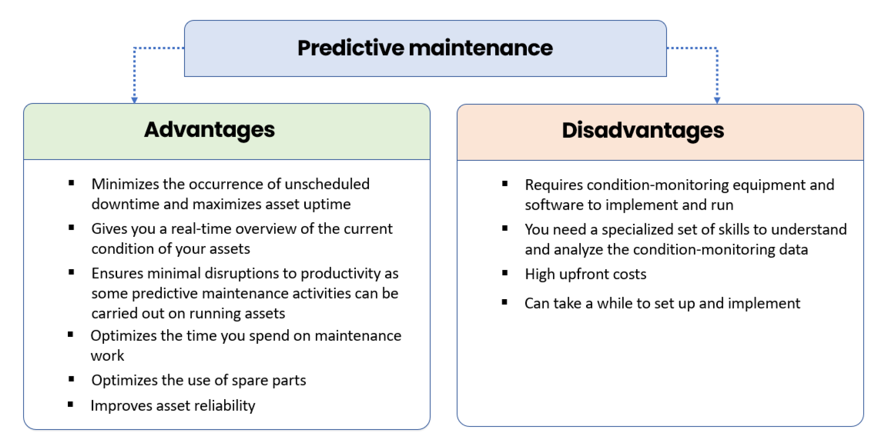
Predictive maintenance benefits and drawbacks:
Predictive maintenance, as with any other maintenance strategy, has advantages and disadvantages (See
Figure 1):
Data analysis is what differentiates preventive maintenance from predictive maintenance. Indeed, three components make up PdM, which allow technicians to monitor the condition of equipment and alert them to upcoming failures [
7]:
Sensors installed in the machine generate real-time data on its health and performance;
The Internet of Things (IoT) connects machines, software, and cloud solutions, enabling the collection and analysis of huge amounts of data;
All the processed data are fed into predictive models, which can predict failures based on that information.
As technology has advanced throughout industrial revolutions, the impact on maintenance strategies and equipment performance has changed, as illustrated in the following table (See
Table 1).
Industry 4.0 is transforming how businesses create, enhance, and distribute their products. By enabling equipment intercommunication through the Internet of Things, big data, computer intelligence, and decision-making systems, it has fundamentally changed the industrial and manufacturing world [
5]. Industry 3.0 has been disrupted by the introduction of computers due to new technologies [
8]. Industry 4.0 enables autonomous decision-making by connecting and communicating with industrial machinery and computers today and in the future.
The Industry 4.0 model suggests the use of multidisciplinary technologies to achieve these advantages and effective factories. Although some of these have been studied for a while, they have not yet reached the point where they can be widely used in industry [
9] (p. 0). In fact, pieces Industry 4.0 equipment are capable of automatic communication with each other, enabling them to coordinate with other remote systems as well as with one another via the internet. As predictive maintenance aims to determine the probability of machine failure occurring, this study attempted to anticipate the failure and determine the type of possible failure by applying machine learning algorithms. This led us to predict the necessary maintenance to be carried out on TA-48 compressors to avoid stoppages and blocking production [
10].
According to the literature [
11], the most important costs come from downtime due to equipment failures, such as compressors. Thus, maintaining production equipment is a key issue for productivity as well as product quality. Equipment maintenance is a combination of technical, administrative, and managerial activities.
To the best of the authors’ knowledge, there is a lack of investigation into automatic solutions through the application of predictive maintenance approaches and Industry 4.0 concepts. The current study provides automatic solutions through the application of predictive maintenance approaches and Industry 4.0 concepts. The originality of this work lies in the construction of a failure prediction model based on machine learning methods. Indeed, the best solution to address this problem is to implement a machine learning model that aims to predict occasional downtime by searching and testing different algorithms through the preparation and processing of data collected by the sensors related to the compressor machine. Aditionally, to help professional users to make decisions, the results were displayed on a Grafana dashboard that allows easily predicting the remaining time until the occurrence of failures on the compressor from the data collected by the sensors.
2. Data and Methods
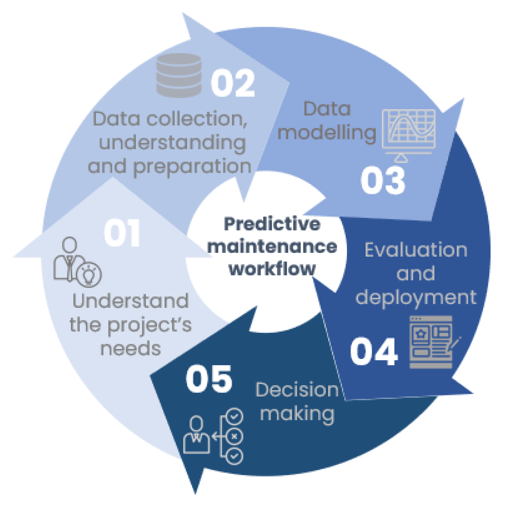
When planning a predictive maintenance project, a life cycle must be followed. Data science and machine learning constitute the process of structuring the solution of a problem using data. An example of predictive maintenance is shown in
Figure 2 [
5]:
Step 1. Analyzing the project’s requirements: To begin, one must understand the business elements, problems, and constraints of a project. This step requires a thorough understanding of both the equipment and systems that are relevant to the project, as well as how they operate. It involves defining the physical quantities to be measured, selecting the sensors, and installing them if necessary. The next step involves defining a list of failure types that may occur.
Step 2. Understanding, collecting, and preparing data:
- →
Data collection: Data can be collected and stored in databases using the sensors in the equipment.
- →
Understanding: During this phase, the data to be analyzed are determined, the quality of the data is identified, and its meaning is related to the data.
- →
Preparation: In this sub-step, related data are selected; data are integrated by merging datasets; missing values are cleaned and managed by deleting them or by calculating them from related datasets; erroneous data are managed by deleting them; outliers are checked and processed; updated data and enhanced features can be obtained by feature engineering, the data can be formatted in the desired structure, and unnecessary columns and features can be removed. Data preparation takes a lot of time and work, typically between 70% and 90% of the project’s total time.
Step 3. Data modeling: In data analysis, data modeling plays a pivotal role. The model receives input data (preparation), and output data are provided. Whether it is a classification problem, a regression problem, or a clustering problem, the first step is to select an algorithm to solve the problem. Different algorithms must be evaluated and parameterized in order to create a model.
Step 4. Evaluation and deployment:
- →
The developed model should not be biased and should be both generalized and have good performance.
- →
During the deployment of the model, each step must be given proper attention, time, and energy.
Step 5. Decision-making: Generally, operators use decision-making processes to decide how to resolve problems. Taking a step-by-step approach to making decisions can assist in making informed, thoughtful decisions that will make a positive difference in the short- and long-term.
In the current study, the steps of the methodology of predictive maintenance workflow were followed, allowing us to explore and process the data intended for the training of the model. Our dataset is a combination of several merged csv files. Indeed, for each variable or attribute recorded by the sensors, we had a csv file with two columns, the first being reserved for the dates and the second for the recorded values of the variable. Thus, a comparative study of the various prediction algorithms was carried out to determine the final choice, which is based on the implementation of the LSTM neural networks. In addition, its performance was improved as the data sets were fed and incremented. Any solution is expected to be improved to maintain its usefulness and performance. Finally, the deployment of the model will allow operators to know the fault times of the compressor and subsequently ensure a minimum downtime rate by making decisions before failures occur.
3. Prediction of Compressor Faults Using Machine Learning Is a Supervised Problem
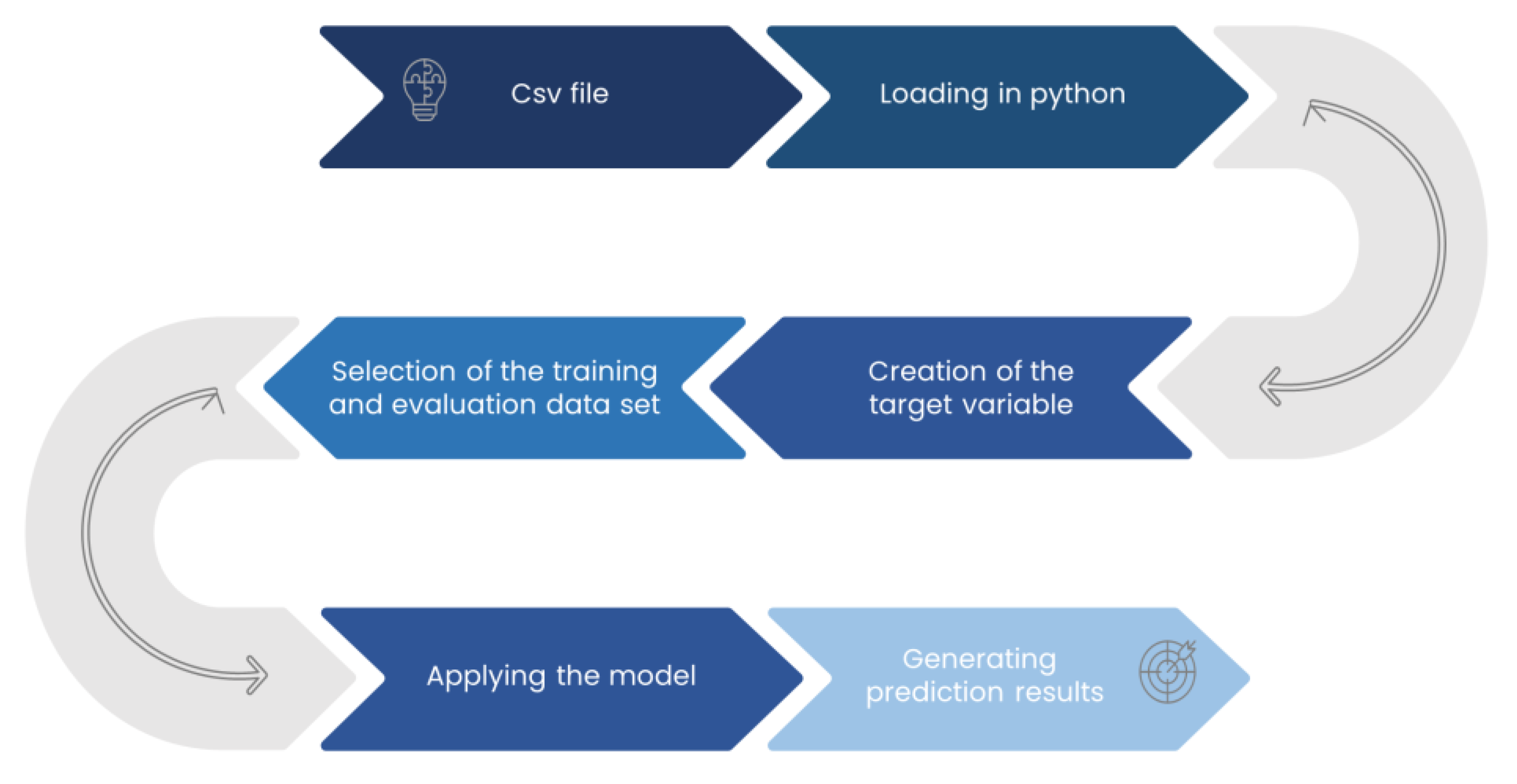
The following procedure for handling the data sets will assist in forecasting future anomalies in the compressor machine and in identifying the target variable and the steps to take to accomplish these aims. The following figure (
Figure 3) provides a general overview of the prediction process.
Regarding the data collection, in this study a set of data collected by sensors linked to the compressor machine recorded hourly voltage, pressure, flow, humidity, temperature, etc. The data understanding phase also includes activities to familiarize oneself with the data, identify data quality issues, gain preliminary insights into the data, or identify interesting subsets to develop hypotheses for hidden information. The data understanding phase starts with initial data collection. The following steps are considered for data processing and understanding [
12].
- →
Data Normalization: Normalization is the process of organizing data in a database. In effect, it is a passive transformation that examines input strings and creates normalized versions of those strings.
- →
Data Cleaning: Data cleaning refers to the process of identifying incorrect, incomplete, inaccurate, irrelevant, or missing portions of data and then modifying, replacing, or deleting them as necessary. Data cleaning is considered a fundamental part of basic data science. In machine learning, if the data are irrelevant or error-prone, it leads to the construction of an incorrect model.
- →
Missing Values: Dealing with missing values is crucial because if they are left unresolved, the analysis and machine learning models will be impacted. Checking to see if the dataset has any missing values is crucial. If so, one of three actions must be taken to solve the issue:
Using Algorithms to Predict the Future
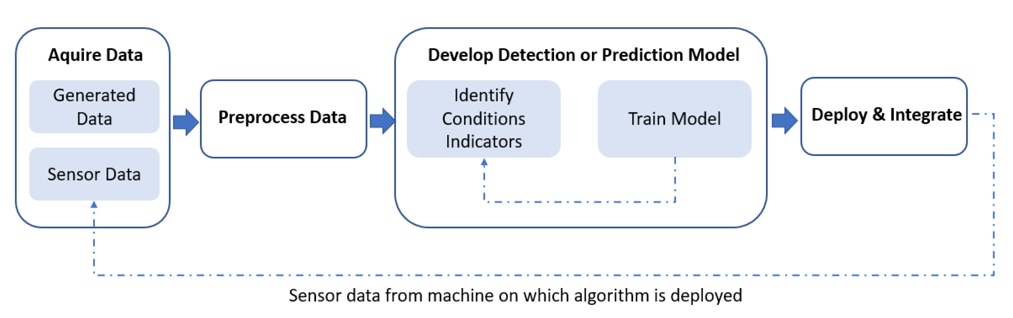
The creation of predictive algorithms, also known as prognostic algorithms, is the most crucial and perhaps most difficult aspect of predictive maintenance. As a result, a model that takes into account a variety of factors and how they interact and affect one another is created in order to predict machine failures. As many variables as possible should be used to increase the precision of the models. Predictive model development is an iterative process as a result. Data from CMMSs, file cabinets, personal observations, FEMA analyses, and internal sensors such as accelerometers and flow meters are gathered for the initial modeling. Condition-monitoring sensors may need to be installed first and operated for a period of time in order to collect baseline data and create the first predictive model (See
Figure 4).
Over time, as more data are generated by the installed sensors, it is possible to improve the initial models and produce near-perfect failure predictions.
Without getting too technical, we here describe how the algorithms work. Based on pre-established rules, their algorithms compare the current behavior of the asset with its expected behavior. A deviation causes a gradual deterioration, which will eventually lead to the failure of the asset. Based on the deviations, current operational circumstances, and historical failure data, the algorithms attempt to predict the points of failure.
Automated systems achieve the following:
- →
Sensors installed in the system monitor operating conditions;
- →
Analyze anomalous data patterns and predicts them;
- →
Detect deviations from thresholds and alerts users.
4. Machine Learning Phase
Machine learning (ML) has emerged as one of the pillars of information technology over the past two decades. There are good reasons to believe that intelligent data analysis will become even more ubiquitous as a necessary ingredient for technological progress, given the ever-increasing amount of data available.
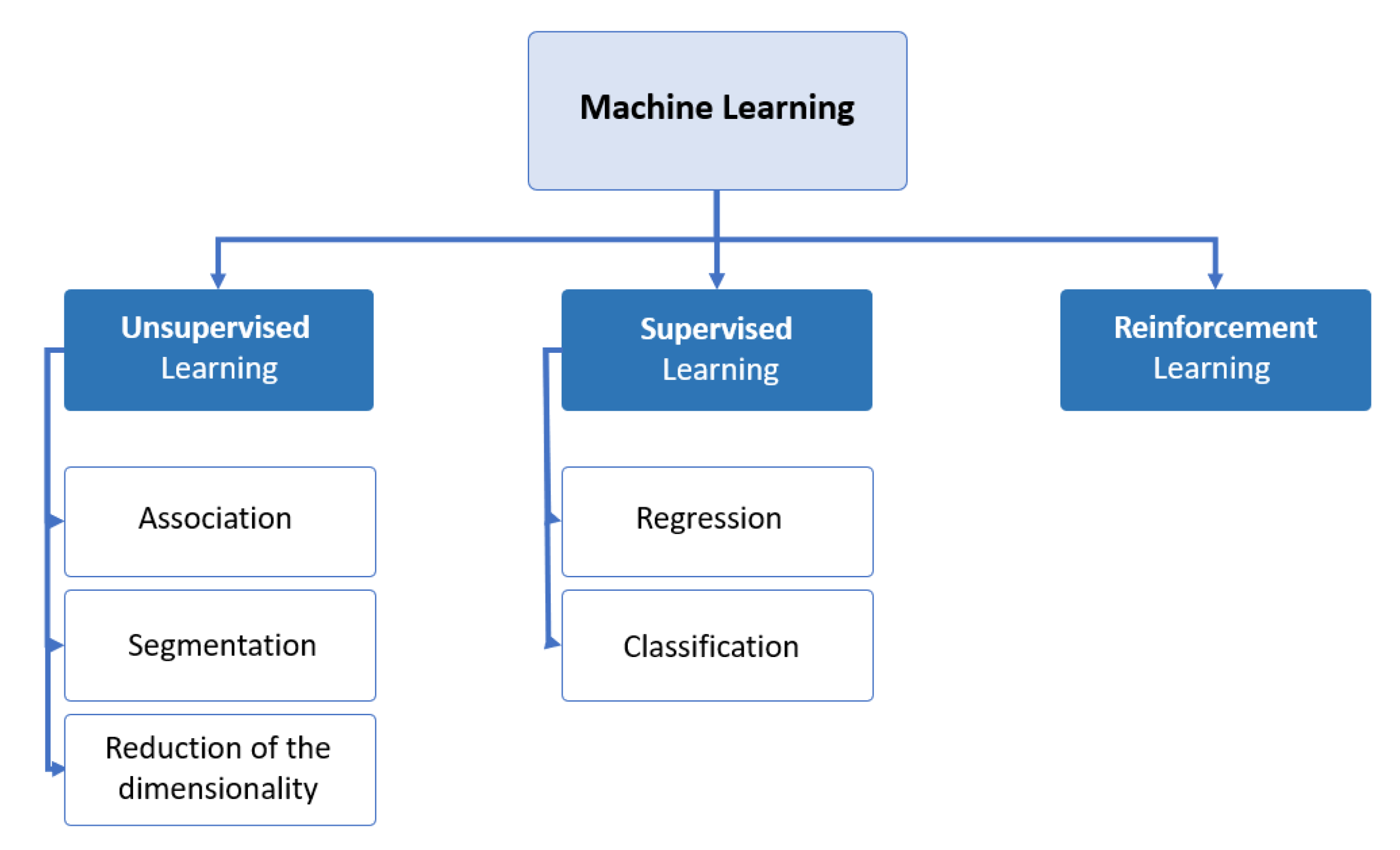
A subset of artificial intelligence (AI) called “machine learning” employs computer algorithms to make independent learning decisions based on data and knowledge. In machine learning, computers do not need to be explicitly programmed, but can modify and improve their algorithms on their own. Today, machine learning algorithms allow computers to communicate with humans, and, for example, to drive cars autonomously. We believe that machine learning will have a huge impact on most industries and the jobs they offer. There are several ways to learn automatically depending on the data, the problem to be solved, and the available data [
13]. The following figure (
Figure 5) summarizes the most popular types of machine learning:
Supervised learning is used in most practical ML applications. An algorithm known as supervised learning begins with a training dataset that contains both the input and output variables [
14]. The matching function between the input and the output is learned using an algorithm. To predict the output variables using new input data, it is necessary to approximate the matching function. Regression and classification problems are two categories of supervised learning issues. Unsupervised learning has no corresponding output variables, only input data. Problems with clustering and feature extraction can be classified as unsupervised learning problems [
15].
The development of algorithms that can create general models and hypotheses using data from external sources to predict the outcome of future instances is known as supervised machine learning [
16].
In most MLSs, trained learning is used. The available data sets are referred to as “true” or “correct” data sets during the learned learning phase. These input data sets, also known as “training data,” are used to “feed” the algorithm [
17].
The algorithm’s tasks during this process are to estimate the experimental input data and then expand or contract the detected estimates using the “ground truth” as a reference. This process is repeated until the algorithm reaches a universally acceptable level of accuracy. The most well-known supervised machine learning algorithms are described in the following paragraphs and are used in the simulation of the results shown below:
- →
Decision Tree: The decision tree creates tree-like models for classification or regression. A decision tree is incrementally developed while a data set is broken down into smaller and smaller subsets. The outcome is a tree with leaf nodes and decision nodes. This technique is used in regression to forecast a quantitative variable’s value based on qualitative and/or quantitative explanatory variables. This method forecasts the class to which the output variable belongs, unlike classification. There are several algorithms that can be used to construct a decision tree: ID3 (Inductive Decision Tree), its successor C4.5, and CART (Classification and Regression Tree) [
18].
- →
Support Vector Machine: Support Vector Machines (SVM) are a group of associated supervised learning techniques used for regression and classification. They are members of the generalized linear classifier family. In other words, they are classification and regression prediction tools that automatically avoid overfitting to the data while maximizing predictive accuracy using machine learning theory. SVMs are systems that employ a linear function’s hypothesis space in a high-dimensional feature space and are trained using algorithms from optimization theory that incorporate learning bias derived from statistical learning theory [
19].
- →
Naive Bayes: Naive Bayes is a straightforward learning algorithm that makes the strong assumption that the attributes are conditionally independent given the class in addition to using Bayes’ rule. Although in practice this independence assumption is frequently broken, Naïve Bayes algorithms still frequently offer competitive classification accuracy. This, along with its computational effectiveness and numerous other appealing characteristics, causes Naïve Bayes to be widely used in practice [
20].
- →
Random Forest: A random forest is an improvement of the bagging algorithm; proposed by Breiman (2001), it is a supervised machine learning algorithm constructed from decision tree algorithms used to address regression and classification problems. An algorithm called a random forest is made up of many decision trees. The random forest algorithm’s “forest” is trained by “bagging” or bootstrap aggregation. An ensemble algorithm called bagging increases the precision of machine learning algorithm [
21].
- →
Logistic Regression: A statistical analysis technique called logistic regression forecasts a data value based on actual observations in a data set. One of the most popular machine learning algorithms is used for binary classification problems, which have two possible values for each class and include predictions such as “yes or no” and “0 or 1”. Estimating event probabilities and establishing a link between individual outcome probabilities and characteristic probabilities are the goals of logistic regression [
22].
Instead of creating physical or statistical models in the industrial domain, AI approaches try to learn the degradation patterns of machines from the data that are currently available. They can handle complex mechanical system prognostic issues whose degradation processes are challenging for physical or statistical models to relate to one another [
23].
- →
Artificial neural network (ANN): An ANN is a type of computer system. It is based on the theories of massive interconnection and parallel processing architecture of biological systems. An ANN is a data-driven mathematical model capable of using machine learning neurons to solve problems. One of the advantages of ANNs is their ability to recognize complex non-linear relationships between inputs and outputs without resorting to physical processes or direct knowledge [
24].
- →
Recurrent Neural Network (RNN): The RNN was initially developed in the 1980s [
25]. An input layer, one or more hidden layers, and an output layer make up its structure. The idea behind RNNs’ chain structures of repeating modules is to use them as memory to store crucial data from earlier processing steps. In fact, RNNs have a feedback loop that enables them to take in a series of inputs. This indicates that the result of step t-1 is fed back into the network to affect the results of steps t and higher [
24].
- →
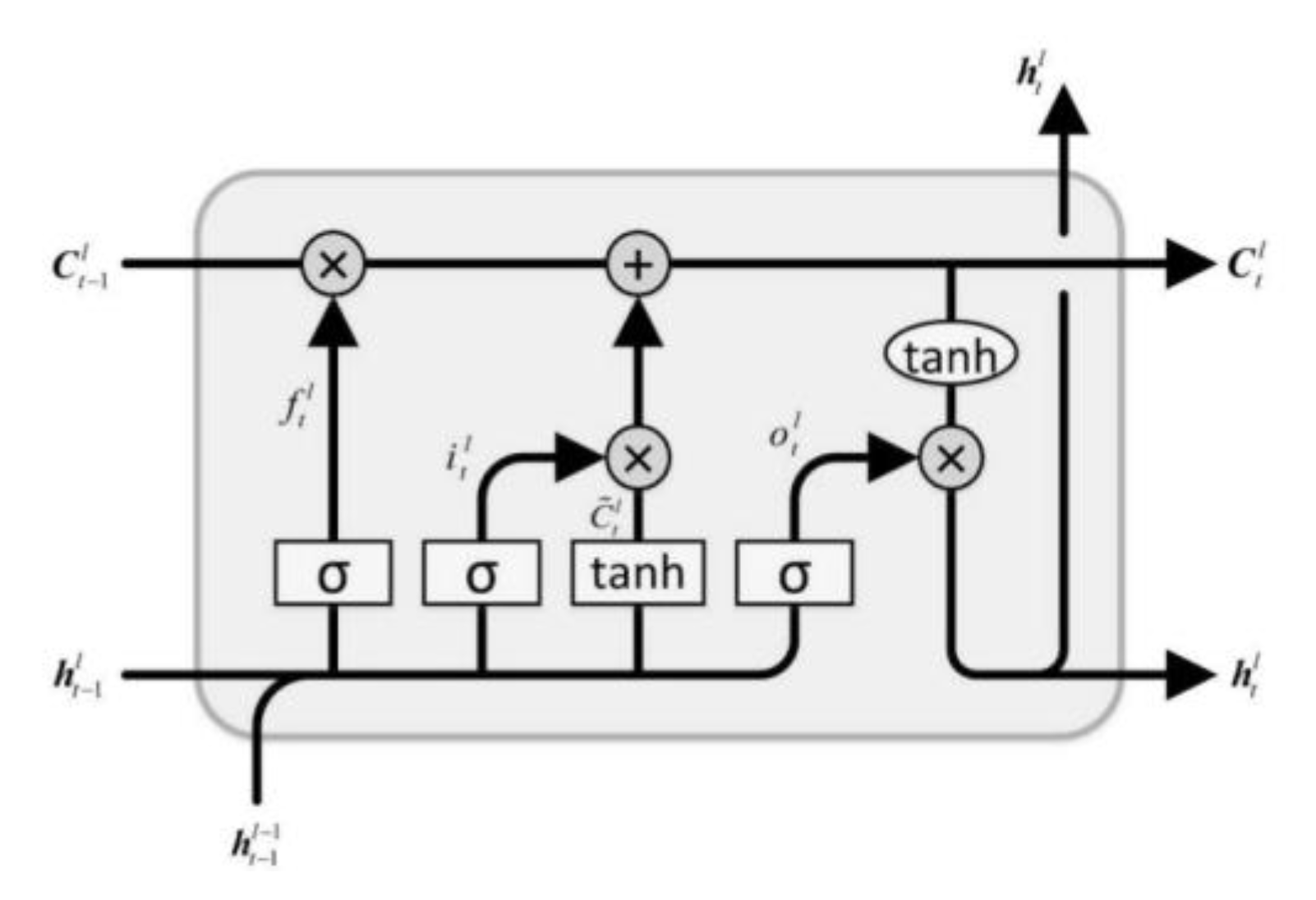
Long Short-Term Memory (LSTM): LSTM is a special RNN has been developed to solve the problem of RNN gradient dispersion. The update and transfer of information between the cells of a LSTM network is described in
Figure 6 below. The state of LSTM cells is different compared with those of RNN networks (See
Figure 5). It consists of a long-term state Ct and a short-term state ht. Three control gates—the forget gate, the input gate, and the output gate—are required for the LSTM cells to change state [
26].
5. Methods Used for Failure Prediction
Based on the literature, there are several methods to follow the failure prediction.
- →
State degradation: This method consists of decomposing the state in the interval between two failures into four states: ‘0’ for the steady state where the compressor works well, ‘1’ for the transient state, ‘2’ means the degradation state, and ‘3’ represents the critical state that leads to the fourth state of the failure.
- →
Setting X hours before the failure occurs: This method involves calculating the probability that the compressor will fail in the next X hours. For this purpose, we take “1” as the state of the failure and for X hours and “0” for the other records.
- →
Remaining life: This method is the most widely used in research [
28]. The remaining useful life is the time the compressor is likely to operate before it requires repair or replacement.
6. Description of the Dataset Used
As previously stated, the study is based on a set of data collected by sensors linked to the compressor machine that records hourly voltage, pressure, flow, etc. These data were gathered in csv files composed of several rows and indexed by the column “Date” which contains dates with consecutive hours.
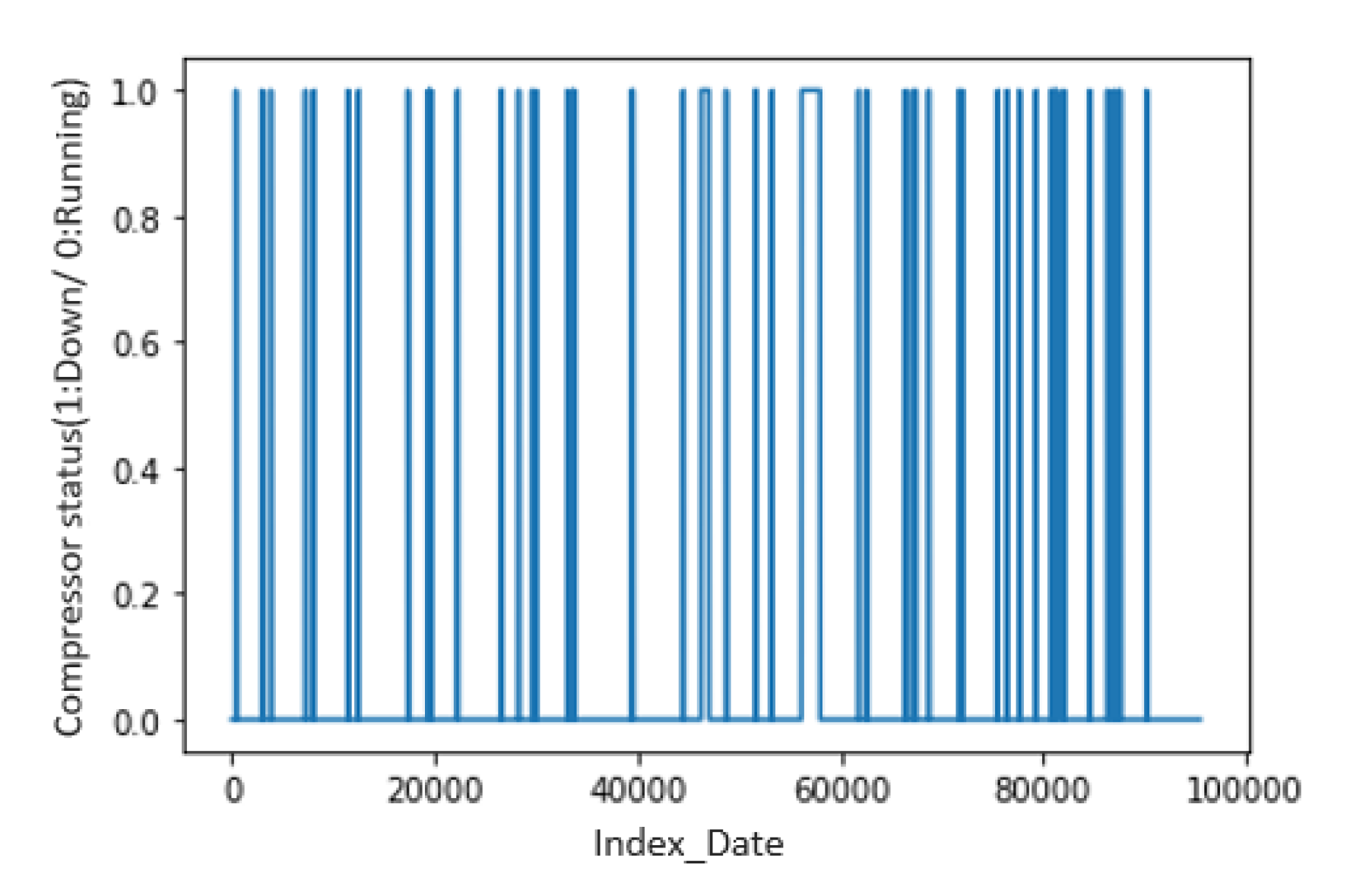
Here, we merged all the variables in a single file which contains, at the beginning, a column reserved for the dates and the rest for our attributes. Then, this file was divided into two sections: one that contained only the variables whose output is a continuous value and the second that contained only the attributes of discrete types. The data were then processed by normalizing and cleaning them as explained above. After merging all the variables and distinguishing the discrete and continuous attributes, we defined the target variable to be predicted later. Indeed, in our dataset we did not find an exact variable that provides the state of operation and which stops the direct compressor. Consequently, we thought of creating this variable, which takes 0 if the compressor is in a working state and 1 in case of stoppage or failure. This variable has the abbreviation CP01. Thus, the target variable was created thanks to two variables: VAR 1, which calculates the flow of the compressor and which must be lower than 2, i.e., so it does not deliver any more air, and VAR 2, which must be on a stop or failure. If both conditions are met, a failure occurs, i.e., CP01 =1, and otherwise CP01 = 0.
The problem of failure prediction is a classification problem since the type of the target variable is a qualitative variable. As a solution, the approach consists of predicting the case where there occur failures at the compressor level. The variable that corresponds to column CP01 is the y of our data set. The following figure (
Figure 7) shows the variable of CP01 indexed by dates. We found 119 failures out of more than 3000 records, the first of which was in 22 August 2010 and lasted almost 8 h.
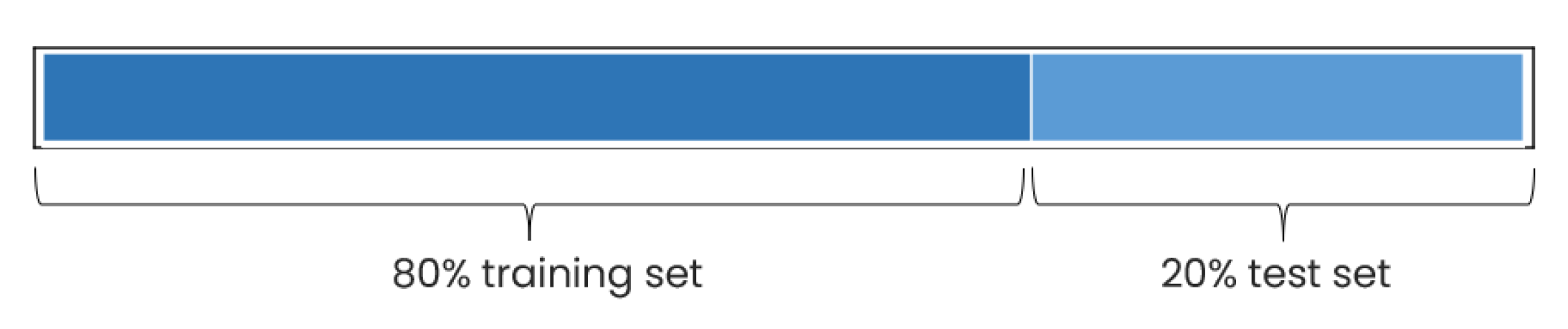
To evaluate the performance of machine learning algorithms when used to make predictions, the dataset was divided into training and test sets. In this way, the results allow for a comparison of the effectiveness of the machine learning algorithms for the given predictive modeling problem. After its designation as a target variable, the two data sets—80% for the training set and 20% for the test set—were constructed. The division of the dataset into training and evaluation is presented in the following figure (
Figure 8).
7. Classification of Failures
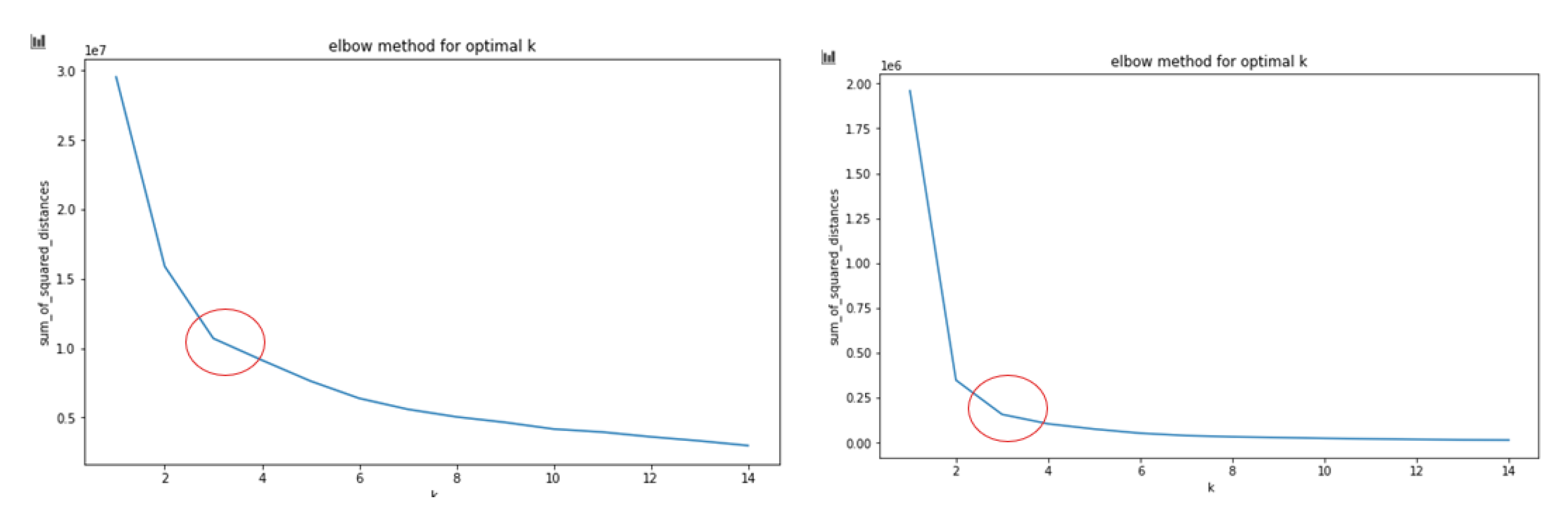
After the preparation of our data, we thought of classifying the data, either continuous or discrete, into clusters that represent the types of failures. Indeed, this step allows maximizing the chances of the machine learning algorithms predicting a failure since it makes the step of learning a type of failure easier than if we opted to predict several different types of failures with different causes. To accomplish this, we used the K-means algorithm, a partition-based cluster analysis technique. It is frequently utilized in cluster analysis because it is more effective, scalable, and quickly converges when working with large data sets [
29]. The elbow method, which involves looking for the point that represents the elbow in a graph that shows the sum of the squared distances between the points and the centers of the clusters to which they belong as a function of the number of clusters chosen, was used to determine the optimal number of clusters K for our dataset [
30]. The results are presented below (
Figure 9).
Therefore, we know that K optimal = 3, and we then applied K-means to have three clusters.
Table 2 shows the percentage of each cluster.
In order to facilitate the resolution of the problem, we followed a precise methodology to achieve our objectives.
After the classification of the failures, we defined three steps for the prediction:
- →
First failure prediction method: prediction of the compressor degradation state (four states: transient to critical);
- →
Second failure prediction method: prediction of the arrival in X hours or method of fixing X (if it is true, there is the arrival of a failure in X hours, and if it is false there occurs no failure in X hours or less);
- →
Third failure prediction method: prediction of the remaining useful life before failure (RUL).
- -
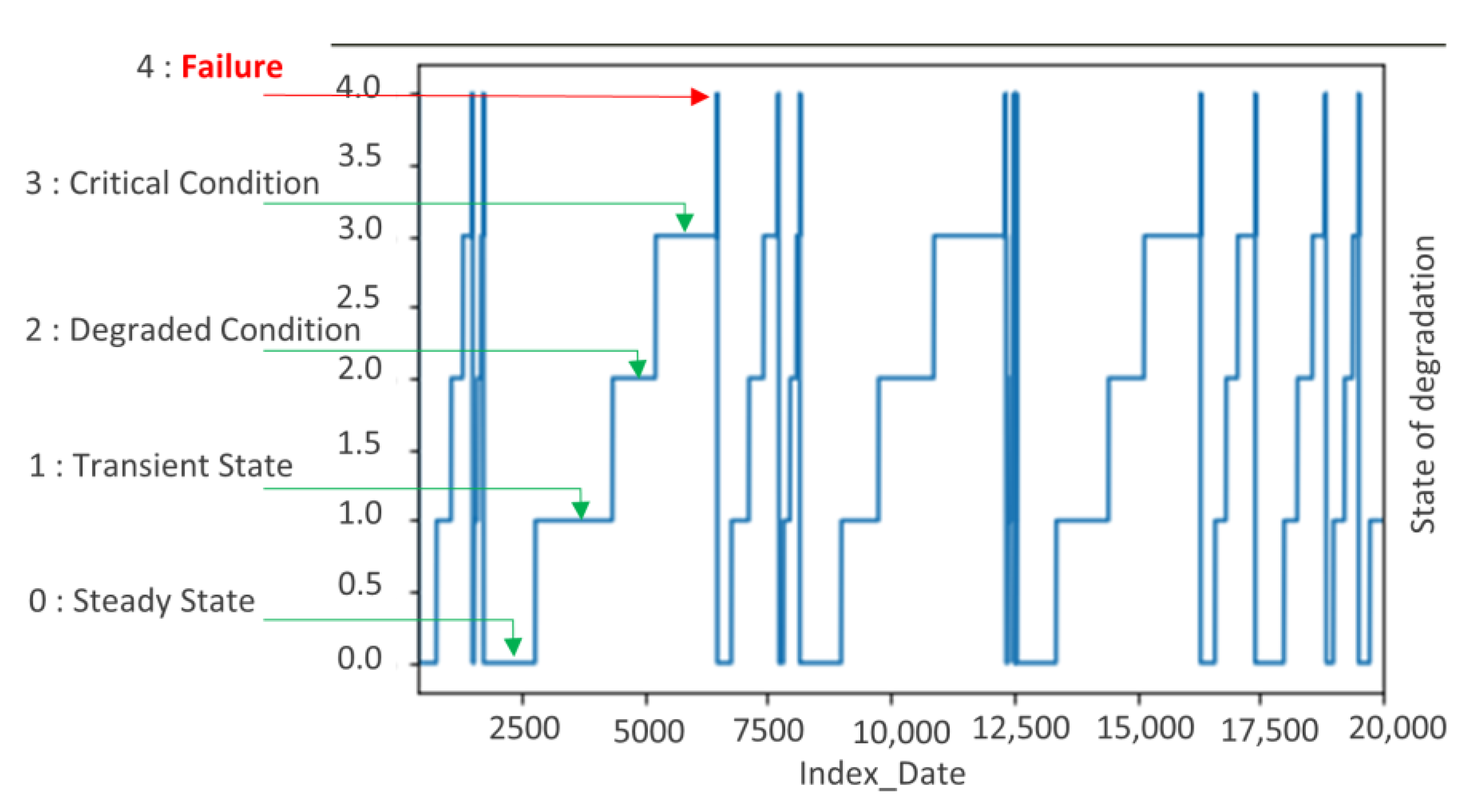
First method of failure prediction: State degradation
This method consists of breaking down the state in the interval between two failures into four states: “0” for the steady state where the compressor is working well, “1” for the transient state, “2” means the degraded state, and “3” represents the critical state that leads to the fourth state of the failure (
Figure 10). To degrade these states, the hierarchical clustering method was used. The latter is a top–down approach where the intervals between failures are treated as a large cluster and the clustering process consists of dividing the large cluster into several smaller clusters. For our case we had five clusters.
- -
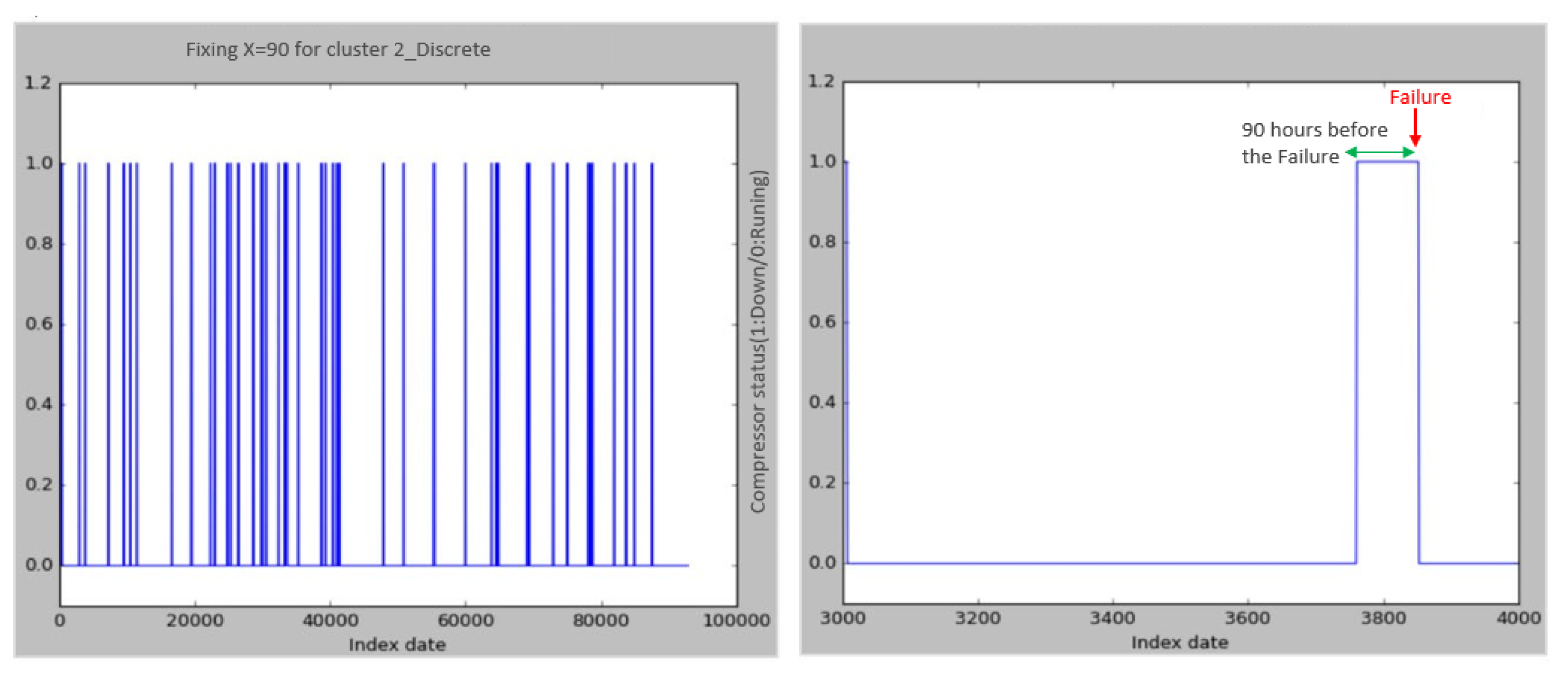
Second method of failure prediction: Fixing X hours before the failure occurs
This method involves the calculation of the probability that the compressor will fail in the next X hours. For this purpose, we set “1” as the state of the failure and for X hours and “0” for the other records. In our case, we tried to predict the X hours that vary between 24 and 500 h in advance. The figure (
Figure 11) below shows an example of cluster 2 of the discrete type for X = 90 h before the arrival of the failure.
- -
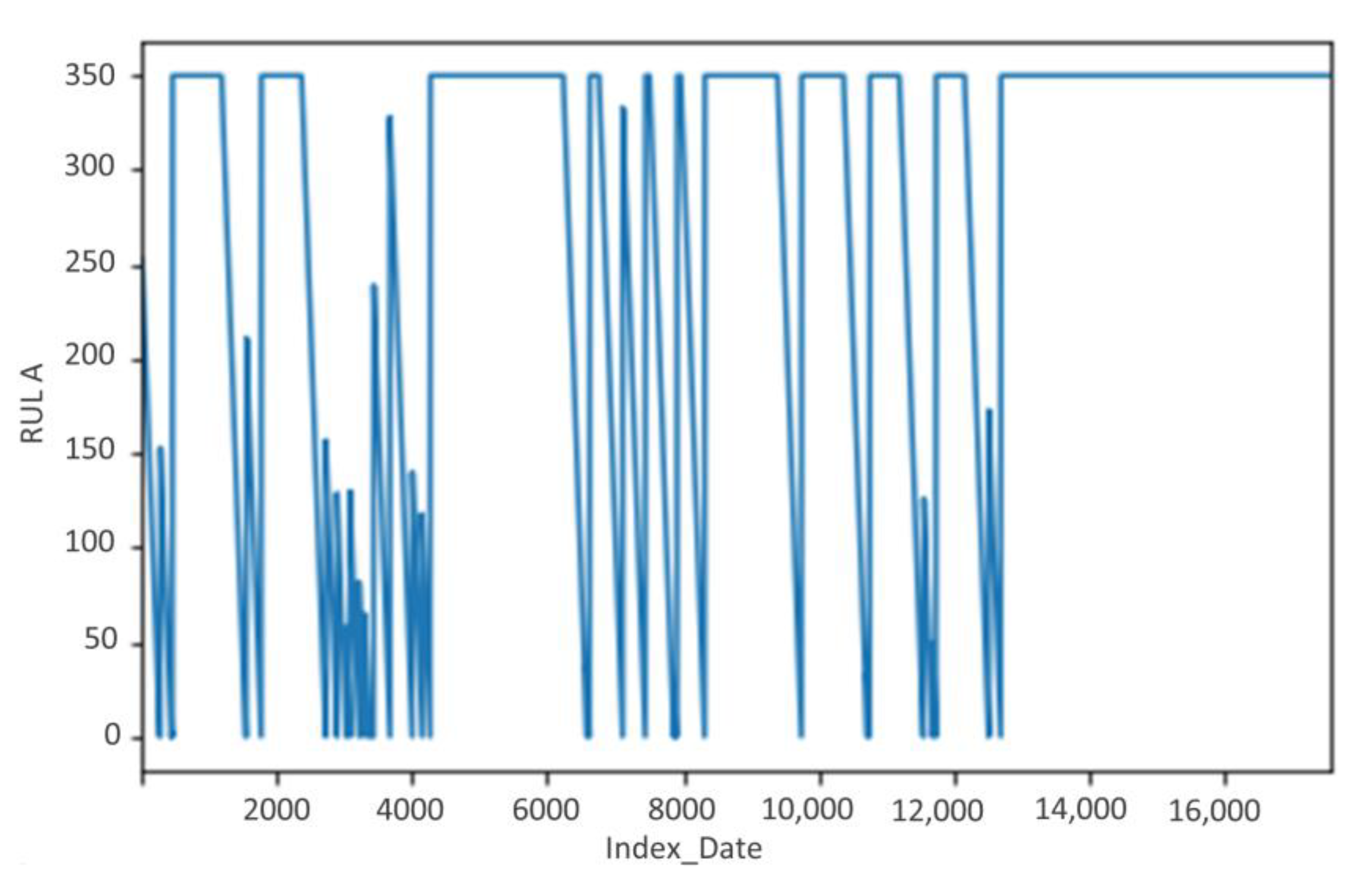
Third method of failure prediction: Remaining life
This method is the most widely used in research [
28]. Indeed, the remaining useful life is the duration during which the compressor is likely to operate before it requires a repair or a replacement. In this sense, we created two other variables: RULA and RULB, which are those we want to predict.
- →
RULA takes the value of “0” for all the records where we have failure, and we dice increment the values from 1 until the value n = 350, which represents 350 h before the arrival of the failure, and we replace the other records that remain with the value 350.
RUL_i_A = 0 to t= failure start date_i
= 1 to t= failure start date_i-1 etc…
Up to n = n to t = failure start date_i-n with n = 350 |
- →
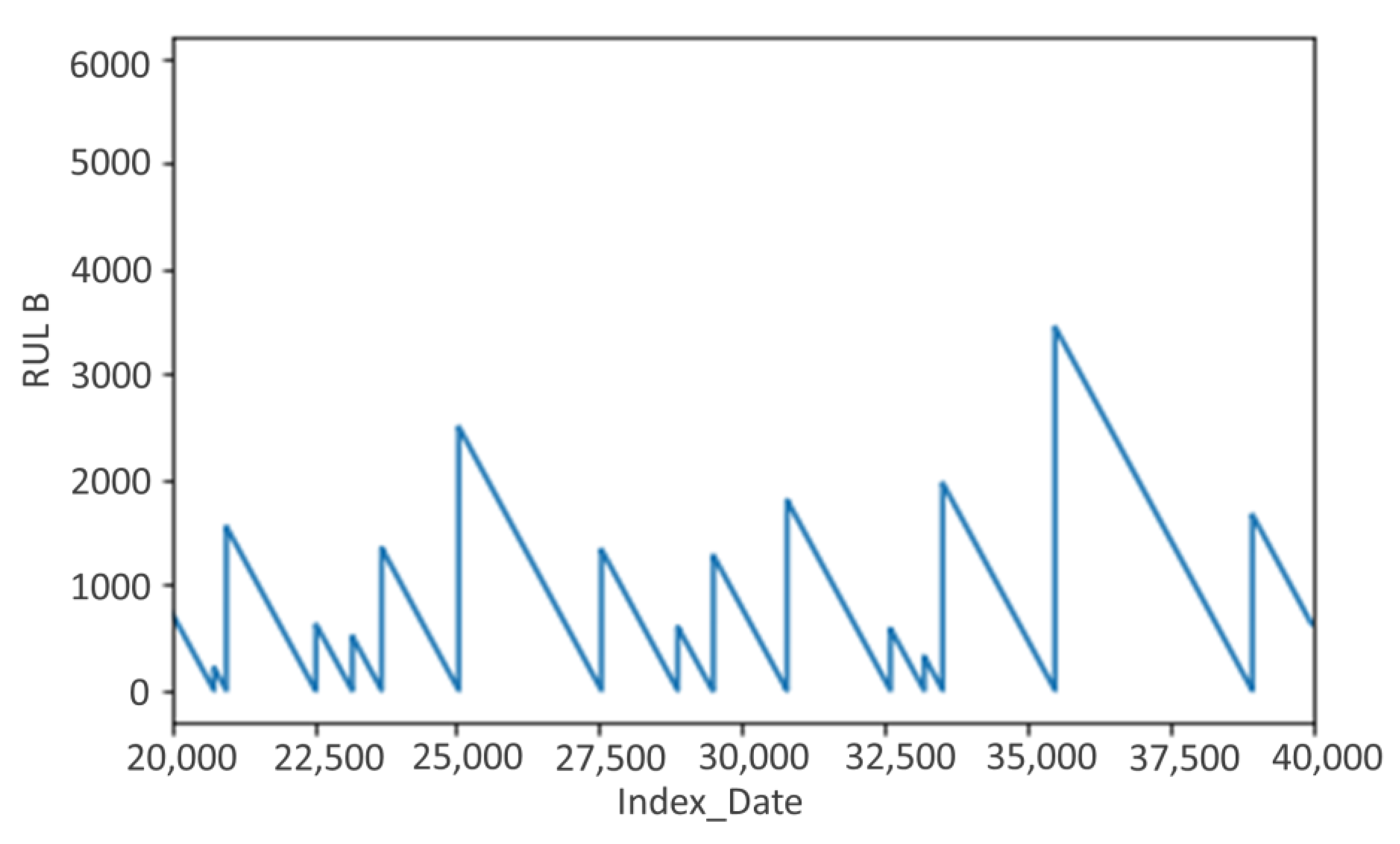
RUL B takes the value “0” for all records where we have failure, and we dice increment the values from 1 to the value n following the record of the failure before.
RUL_i_B = 0 to t= failure start dateI_i
= 1 to t= failure start date_i-1 etc…
Up to n = n to t = failure start date_i-n with n corresponding to the failure end date_(i-1) |
The figure (
Figure 13) below is an overview of RULB.
8. Presentation of Results
8.1. Presentation of Failure Prediction Model Results, Comparisons and Discussions
Two approaches for predicting the target variable CP01 in failure were used: the first was based on machine learning algorithms and the second on time series processes.
8.1.1. Development of the Failure Prediction Model by Using Machine Learning
Method 1: The compressor degradation state prediction method was used for the following algorithms: SVM, logistic regression, and Naïve Bayes.
Table 3 shows an example of discrete cluster 1, which shows the results of the degradation state prediction.
Since the prediction rate obtained was low (did not exceed 30%), the method of fixing X was used.
Method 2: After fixing X hours (with X = 0, 5, 24, 90, 100, and 500), the following learning algorithms were applied to predict the probability that the compressor will fail before these X hours that we fixed.
Table 4 below shows the results found with X= 90, 24, and 0 h before the failure occurred.
Even if we see that the optimal X was 90 h or about 4 days with a success rate for failures, we see that we have only 20% (because 41/(161 + 41) = 0.2). However, this method works very well to detect a failure when it has happened (X = 0 h before the occurrence of a failure).
Method 3: As mentioned before, the objective is to predict the remaining lifetimes for the compressor; to solve this problem, we must first choose suitable estimators, then evaluate these estimators on our dataset, and finally compare the estimators and choose what performs the best. Choosing an estimator to solve a problem is not a simple task. The general objective is to minimize the prediction error; for this, and in order to efficiently predict our variable to be explained, time series and machine learning algorithms were developed, and we present two different types of forecasting techniques. The best-performing technique for the given case study was determined.
Table 5 shows the results found when using the machine learning algorithms. However, these algorithms do not always predict the exact time of the outages, either before or after, and sometimes do not detect that there is a failure for certain types. This led to the use of time series for prediction.
8.1.2. Development of the Failure Prediction Model by Using Time Series
Long Short-Term Memory (LSTM):
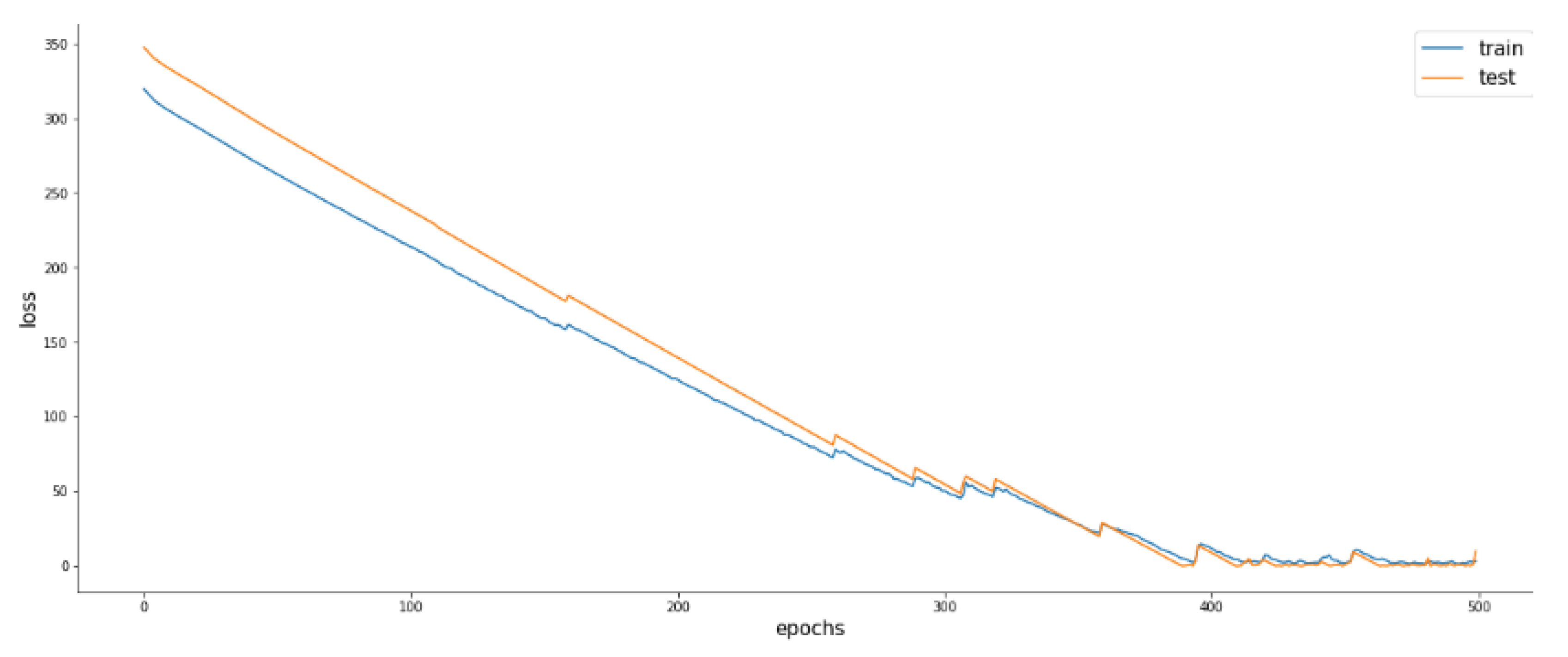
For the purpose of predicting Rul, LSTM was defined with 50 neurons in the first hidden layer and 1 neuron in the output layer. One time step with all features were the input shape. As the loss function, the mean absolute error (MAE) function and the Adam efficient version of stochastic gradient descent were used. The model was fitted to 500 training epochs with a batch size of 4000.
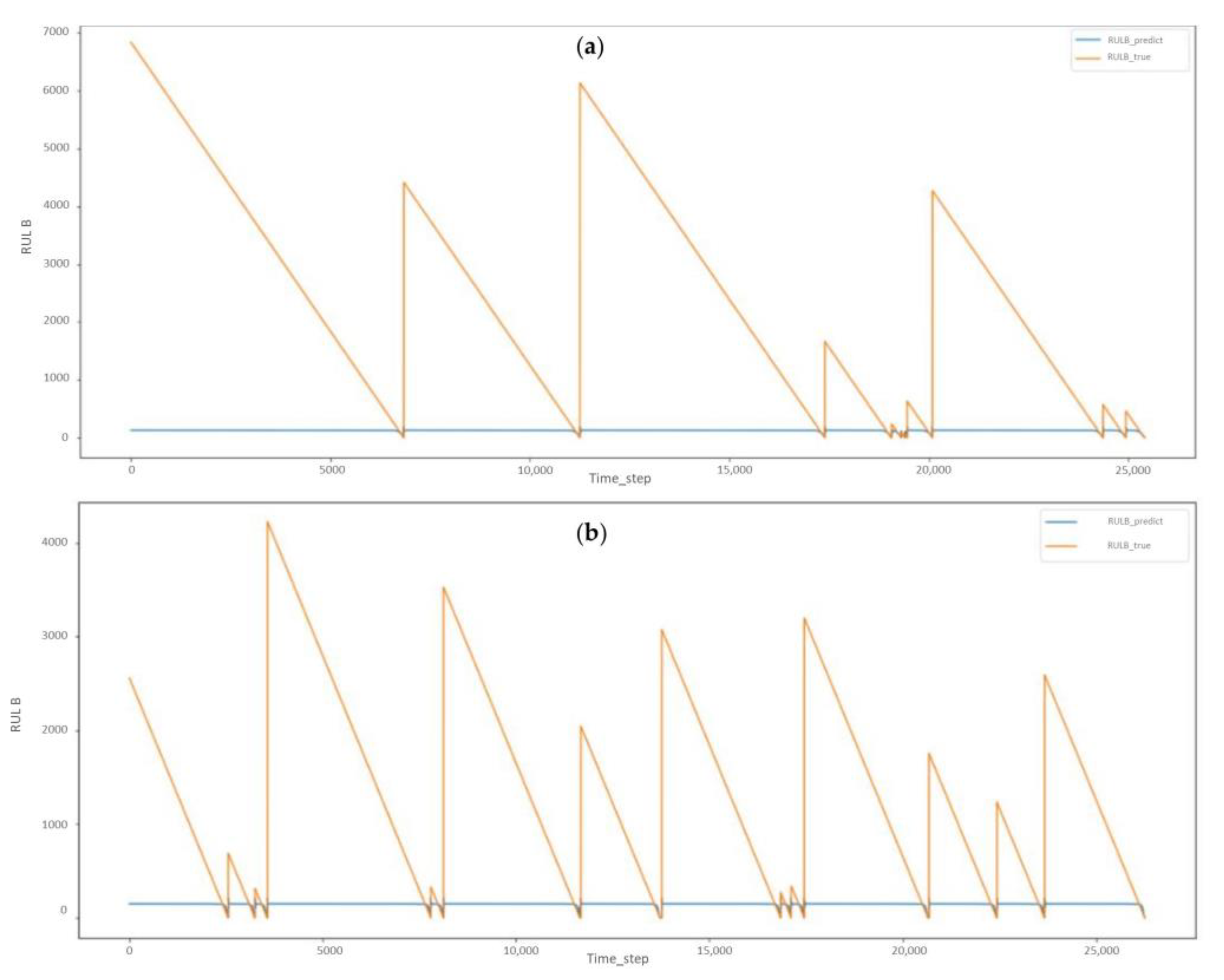
Figure 14 shows the results found by using RUL B for the discrete cluster 1 and 2 failure type.
However, we observed that there was a discrepancy between the predicted value and the actual value in this instance of RULB. This led us to keep the LSTM model only for RULA. The following
Figure 15,
Figure 16 and
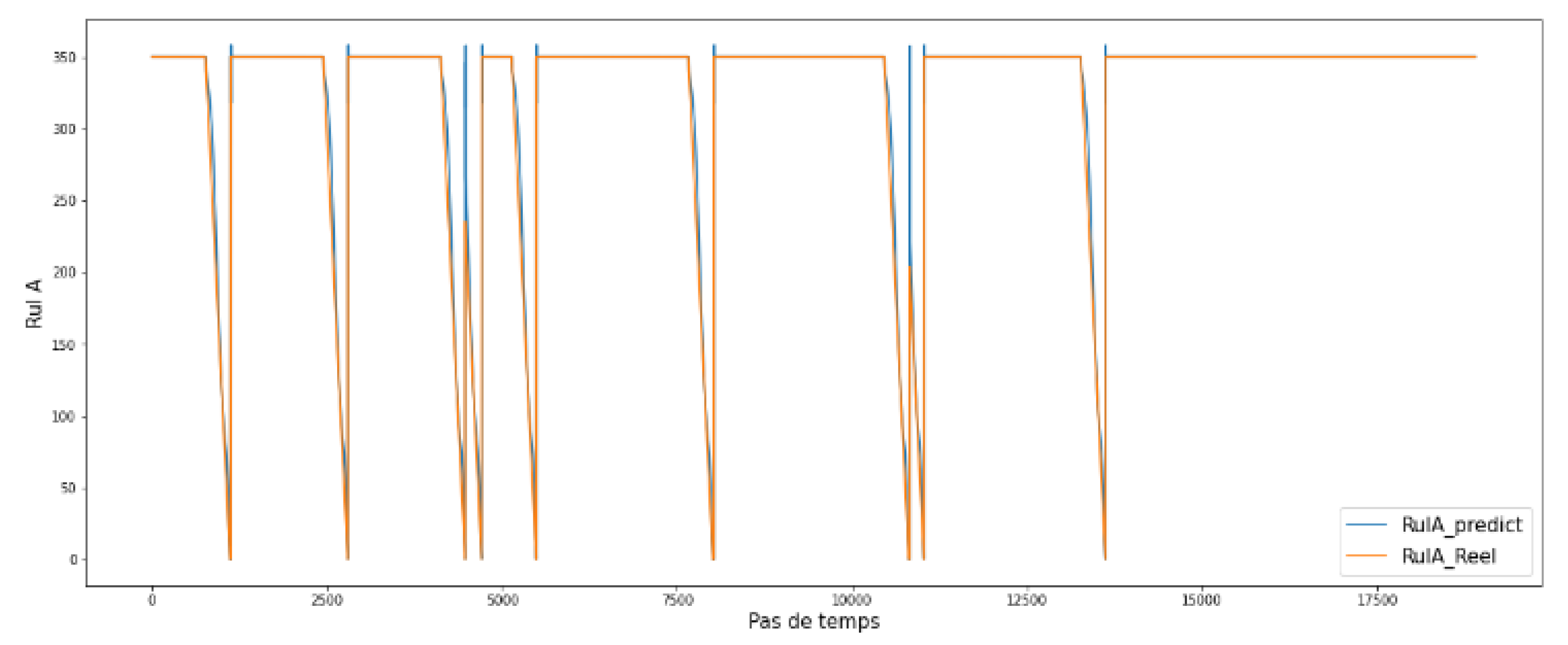
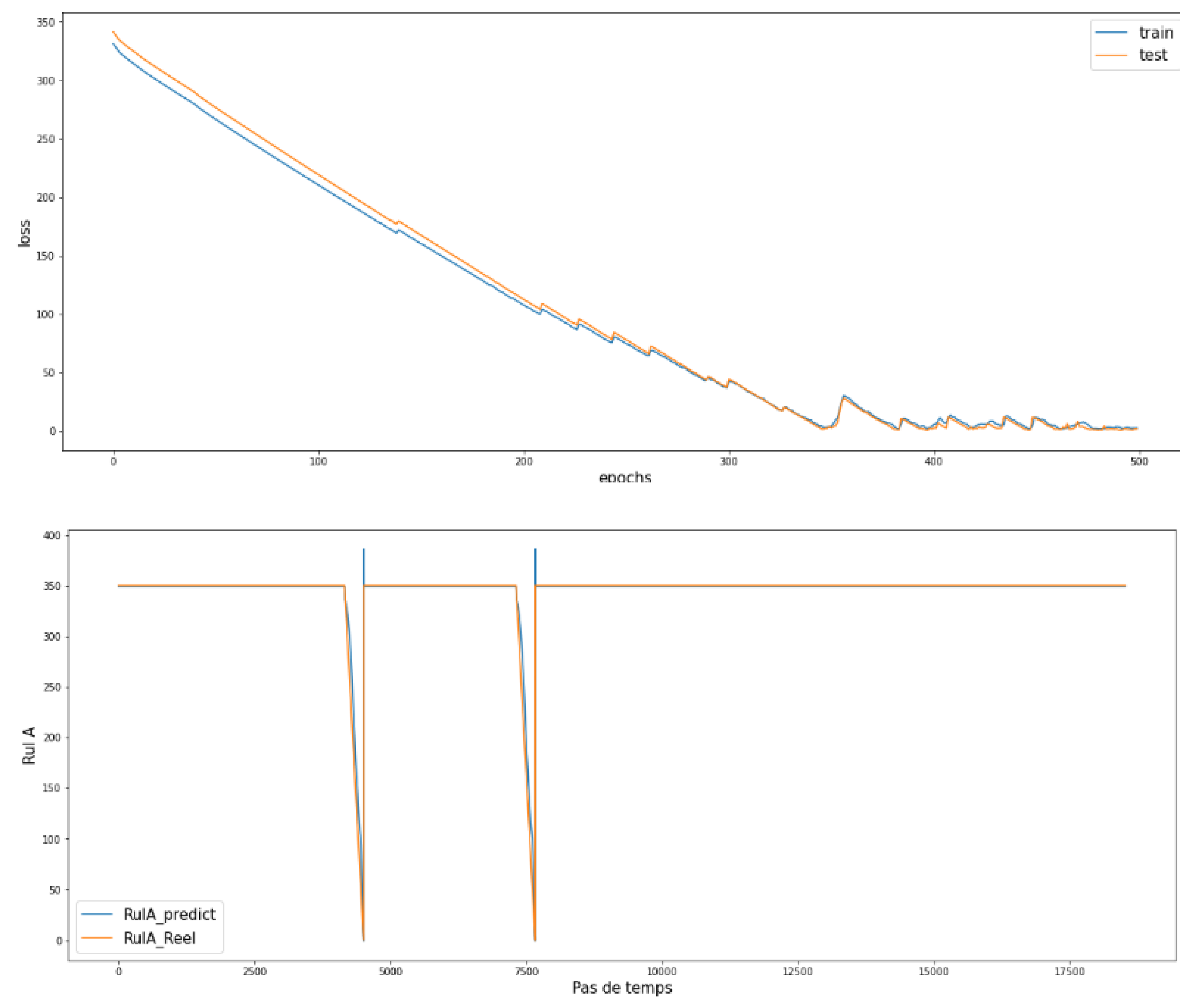
Figure 17 show the results found by using RULA according to the type of continuous failures (1, 2, and 3):
Cluster 1:
Figure 15.
LSTM method for cluster 1 continuous-RULA. Mean squared error = 147.2550818147693.
Figure 15.
LSTM method for cluster 1 continuous-RULA. Mean squared error = 147.2550818147693.
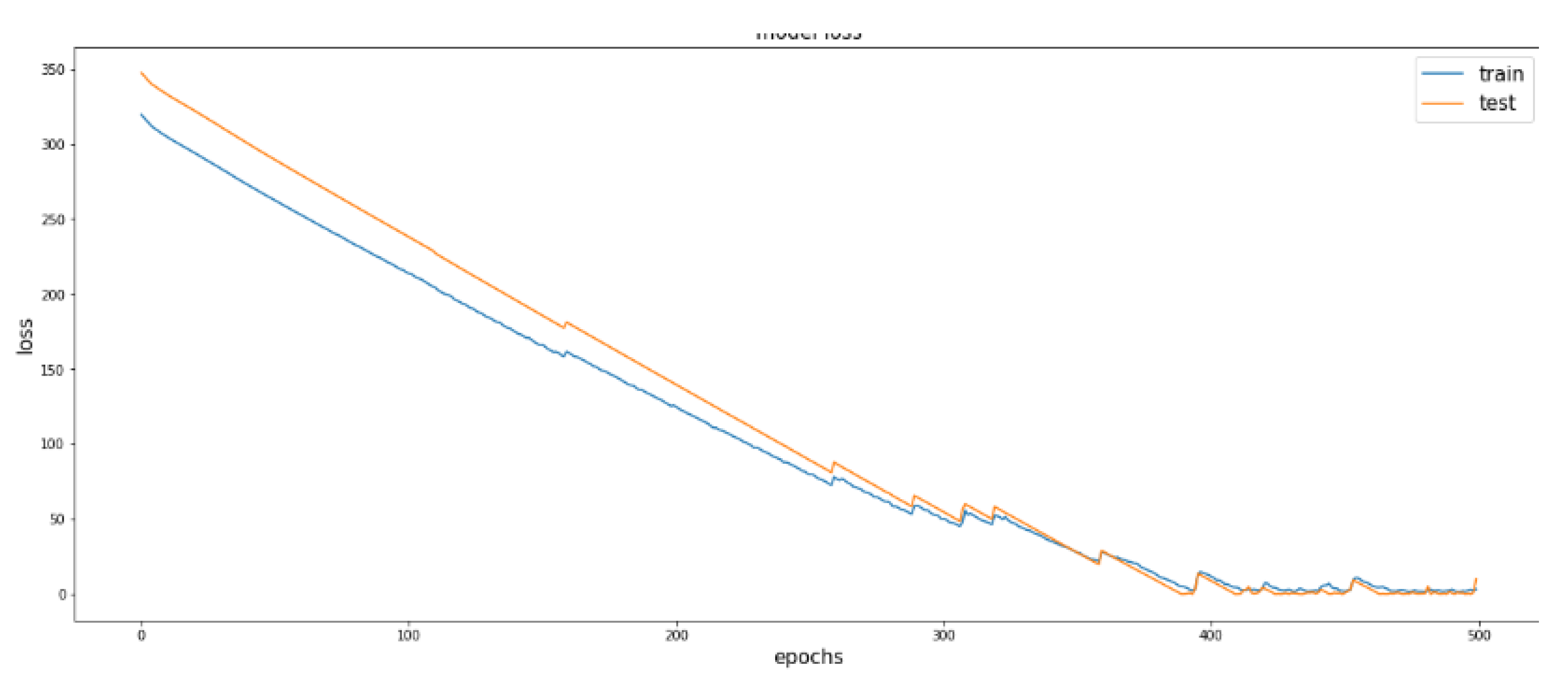
Cluster 2:
Figure 16.
LSTM method for cluster 2 continuous-RULA. Mean squared error = 61.9745811938061.
Figure 16.
LSTM method for cluster 2 continuous-RULA. Mean squared error = 61.9745811938061.
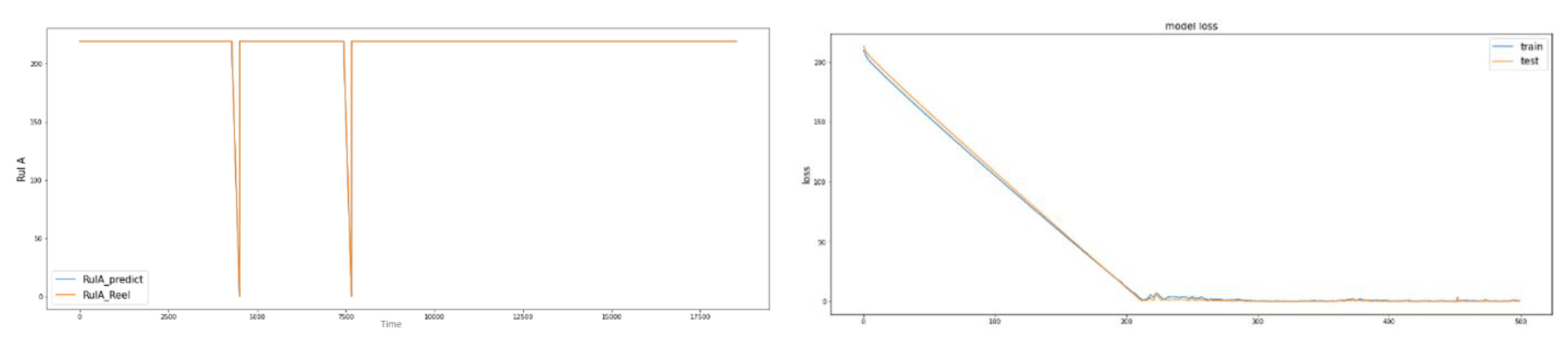
Cluster 3:
Figure 17.
LSTM method for cluster 3 continuous-RULA. Mean squared error = 99.01424394693683.
Figure 17.
LSTM method for cluster 3 continuous-RULA. Mean squared error = 99.01424394693683.
From the figures above, we see that RULA was well predicted compared with RULB. This shows that LSTM is clearly powerful for temporal analysis as well as sequential data. We tried to change the fixed value from RULA= 350 to RULA= 219, and we found a good fit with both continuous and discrete attributes.
Figure 18 shows an example of continuous cluster 2 with RULA= 219.
MSE = 5.354978290025313
Figure 18.
LSTM method for continuous cluster 2 with RULA fixation at 219.
Figure 18.
LSTM method for continuous cluster 2 with RULA fixation at 219.
- ⇒
Final choice for the prediction: The RULA method with LSTM.
A machine learning model can only begin to add value to an organization when the knowledge from that model is regularly made available to the users for whom it was designed. The process involves taking a trained machine learning model and making its predictions available to users or other systems.
8.2. Deployment of the Prediction Algorithm
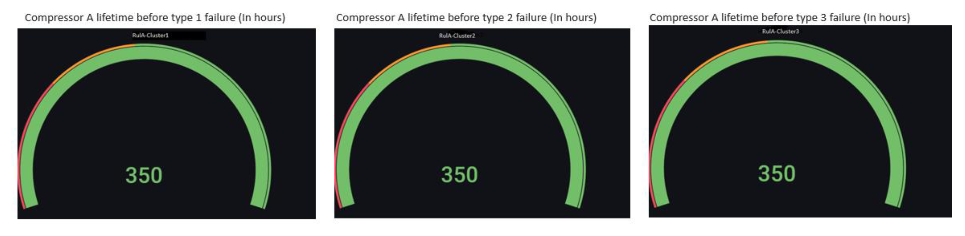
Almost every company has valuable data that internal teams need to access and analyze. Non-technical teams often need the tools to make their jobs easier. Instead of having to query a data scientist for every query, these teams want dynamic dashboards or tools where they can easily run queries and display interactive, custom visualizations. Clean, containerized code is not easy for users to interact with in machine learning models. The easiest way to solve this problem is to place the model behind an API and expose it via interfaces. For the analysis and formatting of the data in the form of counters, graphs, gauges, etc., Grafana is applied. It is a tool for chronological data visualization. It allows creating data representations in a simple interface compatible with Windows, Mac, and Android. Thus, it is arrangeable with several types of databases, including Influx DB. After inserting the dataset containing the RUL, we have access to visualize the gauges of the figure below (
Figure 19), which shows the remaining lifetimes for each cluster we have in the database. The number displayed, “350”, shows that the compressor state is stable and works very well. As time goes by, this number is decremented. Once the value is less than or equal to 210 h, a notification is displayed to warn the operators of the status of the compressor.
9. Conclusions and Perspectives
In this work, we developed a machine learning model for the prediction of the residual life of the compressor machine exploiting machine learning algorithms and time series extracted from the measurements taken online by sensors. Then, to carry out this mission, the workflow methodology was followed with its steps allowing the exploration and processing of the data intended for the training of the model. Thus, a comparative study of the algorithms of prediction of the temporal series was carried out to arrive at the final choice, which is based on the implementation of the LSTM neural networks. This choice will allow the model to be generalized and to adapt to all the machine cases in question. In addition, its performance will be improved over time with the continuous feeding and incrementing of the datasets that are the raw materials of the project. Any solution is expected to be improved in order to maintain its usefulness and performance. Perspectives and improvements to consider are as follows:
- →
Training the model with new observations from the various machine datasets to improve its performance and accuracy (model optimization);
- →
Reducing the dimension of the variables by principal component analysis (PCA);
- →
Deploying the model via a web application to predict the residual life of the compressors after following the same steps for predicting the failure of compressor A.
Author Contributions
Conceptualization, M.A. (Mounia Achouch), H.I., M.A. (Mehdi Adda), M.D. and R.D.; methodology, M.A. (Mounia Achouch), M.D., H.I., S.S.K. and R.D.; validation, H.I., M.D., K.Z., R.D. and S.S.K.; formal analysis, M.A. (Mounia Achouch), H.I., R.D. and M.D.; writing—original draft preparation, M.A. (Mounia Achouch), M.D., A.A. and S.S.K.; writing—review and editing, M.A. (Mounia Achouch), M.D., A.A. and K.Z.; visualization, M.A. (Mounia Achouch), K.Z., R.D. and M.D.; supervision, H.I., M.A. (Mehdi Adda), M.D., R.D. and S.S.K.; project administration, H.I. and M.A. (Mehdi Adda). All authors have read and agreed to the published version of the manuscript.
Funding
This research received no external funding.
Institutional Review Board Statement
Not applicable.
Informed Consent Statement
Not applicable.
Data Availability Statement
The data presented in this study are private.
Conflicts of Interest
The authors declare no conflict of interest.
References
- Benedick, P.-L. Towards a Unified and Robust Data-Driven Approach. A Digital Transformation of Production Plants in the Age of Industry 4.0. Ph.D. Thesis, University of Luxembourg, Esch-sur-Alzette, Luxembourg, 2022. Available online: https://orbilu.uni.lu/handle/10993/50919 (accessed on 14 November 2022).
- Miśkiewicz, R.; Wolniak, R. Practical Application of the Industry 4.0 Concept in a Steel Company. Sustainability 2020, 12, 5776. [Google Scholar] [CrossRef]
- Sajid, S.; Haleem, A.; Bahl, S.; Javaid, M.; Goyal, T.; Mittal, M. Data science applications for predictive maintenance and materials science in context to Industry 4.0. Mater. Today Proc. 2021, 45, 4898–4905. [Google Scholar] [CrossRef]
- Yao, K.; Fan, S.; Wang, Y.; Wan, J.; Yang, D.; Cao, Y. Anomaly detection of steam turbine with hierarchical pre-warning strategy. IET Gener. Transm. Distrib. 2022, 16, 2357–2369. [Google Scholar] [CrossRef]
- Achouch, M.; Dimitrova, M.; Ziane, K.; Sattarpanah Karganroudi, S.; Dhouib, R.; Ibrahim, H.; Adda, M. On Predictive Maintenance in Industry 4.0: Overview, Models, and Challenges. Appl. Sci. 2022, 12, 8081. [Google Scholar] [CrossRef]
- Esteban, A.; Zafra, A.; Ventura, S. Data mining in predictive maintenance systems: A taxonomy and systematic review. WIREs Data Min. Knowl. Discov. 2022, 12, e1471. [Google Scholar] [CrossRef]
- Farahani, S.; Khade, V.; Basu, S.; Pilla, S. A data-driven predictive maintenance framework for injection molding process. J. Manuf. Process. 2022, 80, 887–897. [Google Scholar] [CrossRef]
- Nakayama, R.S.; de Mesquita Spínola, M.; Silva, J.R. Towards I4.0: A comprehensive analysis of evolution from I3.0. Comput. Ind. Eng. 2020, 144, 106453. [Google Scholar] [CrossRef]
- Lasi, H.; Fettke, P.; Kemper, H.-G.; Feld, T.; Hoffmann, M. Industry 4.0. Bus. Inf. Syst. Eng. 2014, 6, 239–242. [Google Scholar] [CrossRef]
- Air Relief. Air Relief Parts List—OEM-Quality Parts Repair Service. Available online: https://www.airrelief.com/general-parts-list/ (accessed on 15 November 2022).
- Bai, C.; Dallasega, P.; Orzes, G.; Sarkis, J. Industry 4.0 technologies assessment: A sustainability perspective. Int. J. Prod. Econ. 2020, 229, 107776. [Google Scholar] [CrossRef]
- Mishra, P.; Biancolillo, A.; Roger, J.M.; Marini, F.; Rutledge, D.N. New data preprocessing trends based on ensemble of multiple preprocessing techniques. TrAC Trends Anal. Chem. 2020, 132, 116045. [Google Scholar] [CrossRef]
- Nacchia, M.; Fruggiero, F.; Lambiase, A.; Bruton, K. A Systematic Mapping of the Advancing Use of Machine Learning Techniques for Predictive Maintenance in the Manufacturing Sector. Appl. Sci. 2021, 11, 2546. [Google Scholar] [CrossRef]
- Abdulqader, D.M.; Abdulazeez, A.M.; Zeebaree, D.Q. Machine Learning Supervised Algorithms of Gene Selection: A Review. Mach. Learn. 2020, 62, 233–244. [Google Scholar]
- Sarker, I.H. Machine Learning: Algorithms, Real-World Applications and Research Directions. SN Comput. Sci. 2021, 2, 160. [Google Scholar] [CrossRef]
- Jiang, T.; Gradus, J.L.; Rosellini, A.J. Supervised Machine Learning: A Brief Primer. Behav. Ther. 2020, 51, 675–687. [Google Scholar] [CrossRef] [PubMed]
- Bzdok, D.; Krzywinski, M.; Altman, N. Machine learning: A primer. Nat. Methods 2017, 14, 1119–1120. [Google Scholar] [CrossRef] [PubMed]
- Ali, J.; Khan, R.; Ahmad, N.; Maqsood, I. Random Forests and Decision Trees. Int. J. Comput. Sci. Issues 2012, 9, 272. [Google Scholar]
- Jakkula, V. Tutorial on Support Vector Machine (SVM). Sch. EECS Wash. State Univ. 2006, 37, 121–167. [Google Scholar]
- Webb, G. Naïve Bayes. In Encyclopedia of Machine Learning and Data Science; Springer: Berlin/Heidelberg, Germany, 2016; pp. 1–2. [Google Scholar] [CrossRef]
- Schonlau, M.; Zou, R.Y. The random forest algorithm for statistical learning. Stata J. 2020, 20, 3–29. [Google Scholar] [CrossRef]
- Kirasich, K.; Smith, T.; Sadler, B. Random Forest vs Logistic Regression: Binary Classification for Heterogeneous Datasets. SMU Data Sci. Rev. 2018, 1, 9. [Google Scholar]
- Lei, Y.; Li, N.; Guo, L.; Li, N.; Yan, T.; Lin, J. Machinery health prognostics: A systematic review from data acquisition to RUL prediction. Mech. Syst. Signal Process. 2018, 104, 799–834. [Google Scholar] [CrossRef]
- Le, X.H.; Ho, H.V.; Lee, G.; Jung, S. Application of Long Short-Term Memory (LSTM) Neural Network for Flood Forecasting. Water 2019, 11, 1387. [Google Scholar] [CrossRef] [Green Version]
- Rumelhart, D.E.; Hinton, G.E.; Williams, R.J. Learning representations by back-propagating errors. Nature 1986, 323, 533–536. [Google Scholar] [CrossRef]
- Li, J.; Li, X.; He, D. A Directed Acyclic Graph Network Combined With CNN and LSTM for Remaining Useful Life Prediction. IEEE Access 2019, 7, 75464–75475. [Google Scholar] [CrossRef]
- Almosova, A.; Andresen, N. Nonlinear inflation forecasting with recurrent neural networks. J. Forecast. 2023, 42, 240–259. [Google Scholar] [CrossRef]
- Si, X.S.; Wang, W.; Hu, C.H.; Zhou, D.H. Remaining useful life estimation—A review on the statistical data driven approaches. Eur. J. Oper. Res. 2011, 213, 1–14. [Google Scholar] [CrossRef]
- Wang, J.; Su, X. An Improved K-Means Clustering Algorithm. In Proceedings of the 2011 IEEE 3rd International Conference on Communication Software and Networks, Xi’an, China, 27–29 May 2011; pp. 44–46. [Google Scholar] [CrossRef]
- Bholowalia, P.; Kumar, A. EBK-Means: A Clustering Technique based on Elbow Method and K-Means in WSN. Int. J. Comput. Appl. 2014, 105, 17–24. [Google Scholar]
Figure 1.
Advantages and disadvantages of predictive maintenance.
Figure 1.
Advantages and disadvantages of predictive maintenance.
Figure 2.
Predictive maintenance workflow.
Figure 2.
Predictive maintenance workflow.
Figure 3.
Description of the existing prediction process.
Figure 3.
Description of the existing prediction process.
Figure 4.
Prediction process.
Figure 4.
Prediction process.
Figure 5.
Machine learning classifications [
13].
Figure 5.
Machine learning classifications [
13].
Figure 6.
Diagram of a LSTM cell [
27].
Figure 6.
Diagram of a LSTM cell [
27].
Figure 7.
Compressor status: running and down.
Figure 7.
Compressor status: running and down.
Figure 8.
The data set for training and testing.
Figure 8.
The data set for training and testing.
Figure 9.
Result of the elbow method for continuous variables (left) and for discrete variables (right).
Figure 9.
Result of the elbow method for continuous variables (left) and for discrete variables (right).
Figure 10.
Degradation of the compressor condition.
Figure 10.
Degradation of the compressor condition.
Figure 11.
Example of the fixing method for X = 90 h for the 2-discrete cluster.
Figure 11.
Example of the fixing method for X = 90 h for the 2-discrete cluster.
Figure 12.
Example of RULA for cluster 1 continuous as a function of the number of hours remaining.
Figure 12.
Example of RULA for cluster 1 continuous as a function of the number of hours remaining.
Figure 13.
Example of RULB for cluster 1 continuous as a function of the number of hours remaining.
Figure 13.
Example of RULB for cluster 1 continuous as a function of the number of hours remaining.
Figure 14.
(a) LSTM method for discrete-RULB cluster 2; (b) LSTM Method for discrete-RULB cluster 1.
Figure 14.
(a) LSTM method for discrete-RULB cluster 2; (b) LSTM Method for discrete-RULB cluster 1.
Figure 19.
Fault-type gauge.
Figure 19.
Fault-type gauge.
Table 1.
The industrial revolution.
Table 1.
The industrial revolution.
| Industrial Revolution | Industry 1.0 | Industry 2.0 | Industry 3.0 | Industry 4.0 |
|---|
| Technological Innovation | Mechanization, steam power | Mass production, electrical energy | Automatization, computer power | Digital solutions, IoT cloud systems |
| Maintenance Policy | Reactive maintenance | Preventive
maintenance | Preventive
maintenance | Predictive
maintenance |
| Technology | Visual Inspection | Instrumental Inspection | Sensor monitoring | Sensing data and predictive maintenance |
| Overall Equipment Effectiveness | <50% | 50–70% | 70–90% | >90% |
Table 2.
K-means results.
Table 2.
K-means results.
| | Cluster 0 | Cluster 1 | Cluster 2 |
|---|
| Continuous Variables | 84.36% | 4.87% | 10.76% |
| Discrete Variables | 10.9% | 82.13% | 6.95% |
Table 3.
The results of the prediction of the degradation state (example of cluster 1) for the three algorithms.
Table 4.
The results of the prediction by fixation of 90 h, 24 h, and 0 h before the failure (example of discrete cluster 1) for the three algorithms.
Table 5.
The results of the prediction by the RUL method.
| Disclaimer/Publisher’s Note: The statements, opinions and data contained in all publications are solely those of the individual author(s) and contributor(s) and not of MDPI and/or the editor(s). MDPI and/or the editor(s) disclaim responsibility for any injury to people or property resulting from any ideas, methods, instructions or products referred to in the content. |
© 2023 by the authors. Licensee MDPI, Basel, Switzerland. This article is an open access article distributed under the terms and conditions of the Creative Commons Attribution (CC BY) license (https://creativecommons.org/licenses/by/4.0/).

 ,
, 


