
Design and Validation of a U-Net-Based Algorithm for Star Sensor Image Segmentation


School of Aerospace Engineering, Sapienza University of Rome, 00138 Roma, Italy
*
Author to whom correspondence should be addressed.
Appl. Sci. 2023, 13(3), 1947; https://0-doi-org.brum.beds.ac.uk/10.3390/app13031947
Submission received: 29 November 2022
/
Revised: 15 January 2023
/
Accepted: 27 January 2023
/
Published: 2 February 2023
(This article belongs to the Special Issue Small Satellites Missions and Applications)
Abstract
:The present work focuses on the investigation of an artificial intelligence (AI) algorithm for brightest objects segmentation in night sky images’ field of view (FOV). This task is mandatory for many applications that want to focus on the brightest objects in an optical sensor image with a particular shape: point-like or streak. The algorithm is developed as a dedicated application for star sensors both for attitude determination (AD) and onboard space surveillance and tracking (SST) tasks. Indeed, in the former, the brightest objects of most concern are stars, while in the latter they are resident space objects (RSOs). Focusing attention on these shapes, an AI-based segmentation approach can be investigated. This will be carried out by designing, developing and testing a convolutional neural network (CNN)-based algorithm. In particular, a U-Net will be used to tackle this problem. A dataset for the design process of the algorithm, network training and tests is created using both real and simulated images. In the end, comparison with traditional segmentation algorithms will be performed, and results will be presented and discussed together with the proposal of an electro-optical payload for a small satellite for an in-orbit validation (IOV) mission.
1. Introduction
In the framework of on-board autonomous star sensors algorithms, star segmentation and accurate centroid estimation are critical problems to face. The number of actual detected stars and the relative centroids’ estimation accuracy have a huge impact on the success of star-identification-based attitude determination routines [1,2]. Taking into account that star sensor images generally contain several noise sources (stray light noise, single point noise, single events upsets (SEUs) and so on), good initial processing of image data is mandatory. In this way, it is possible to improve the percentage of success in the star identification process [3,4] and the possibility of retrieving accurate attitude information from images. A good image segmentation process is also needed for RSO detection, where often the image noise and the weak nature of an RSO streak can lead to an incorrect detection of the object and loss of precious information for the orbit determination (OD) modules.
The process of image segmentation is needed to highlight the useful image information which is geometrically encoded in the image pixels. Often, not all the pixels in an image are needed, and a process of selection and exclusion is mandatory to focus attention on just that image part. Image segmentation faces and solves this problem bringing as a result a binarized image which is often called Mask. Through the convolution of this Mask with the original image, it is possible to extract photometric and geometrical information about the target pixels. In this case, we will not be interested in the photometric information, but this will be discussed in the next sections.
Regarding image segmentation, in the last decades several traditional approaches have been proposed, classified according to the element they take into account to discern foreground and background pixels: image histograms, detection of image gradients, detection of object edges and complexity analysis techniques [1].
Among them, commonly used methods are the following:
- Iterative threshold method [5]: It performs an iterative optimization. An initial threshold is set, and then the algorithm improves the estimation at every step with a suitable improvement strategy. The strategy should be fast enough in convergence and should improve the quality of the segmented image at each step.
- Local threshold methods: They are based on the selection of an initial threshold value plus a margin. For a generic examined pixel, its value is compared with a reference one. This reference value is updated continuously and takes into account the local energy value of the surrounding pixels in such a fashion that characterizes the method. A local threshold method is described in [6], and it is based on a moving streak average, while in [7], the approach uses rectangular areas and the local contrast level.
- Otsu’s algorithm [8]: It performs a more refined approach where the intraclass variance of the foreground and background pixels is considered as a cost index and where the selected threshold comes from its maximization.
- Niblack’s method [9]: It is a localized thresholding algorithm in which the threshold is varied across the image as a function of the local intensity average and standard deviation.
Each reported traditional method presents limitations. Iterative threshold methods rely on all the energy levels in the global image, and these constitute their limit: a simple strong stray-light scenario can badly affect the predictions of these methods. Moreover, when the histogram of a star image is unimodal, the traditional iterative threshold method is time-consuming and cannot reach a suitable segmentation. A local threshold method would fail in the same way if the difference between the star signal and the local noise intensity is lower than the margin. The Otsu method, instead, can only provide satisfactory results for thresholding if the histogram is not unimodal or close to unimodal [10]. Artificial intelligence could be an appealing and useful tool to face this challenging problems due to the recent development and application of AI in image processing.
Star segmentation is a task that has many aspects in common with the segmentation of dim small targets, whose primary goal is to enhance the contrast between the target itself and the background, regardless of its nature; segmentation must be performed in every possible situation (noise, blurring, angular motion of the camera and/or motion of the target).
All these issues also occur in star tracker images. Dim small target segmentation has been studied for both synthetic aperture radar (SAR) and optical images. Jin et al. [11] proposed the application of a lightweight patch-to-pixel (P2P) CNN for ship detection in PolSAR (polarimetric SAR) images. Their approach prefers the use of dilated convolutional layers rather than conventional convolutional layers in order to expand the receptive field without adding any model parameter. Zhao and Jia [12] employed a more general-purpose target segmentation using a CNN on infrared images, testing it on both real and synthetic images; however, their study suffers from the necessity for a large amount of training data to be fed to the network. Fan et al. [13] overcame the issue of large training data by using the MNIST [14] database in such a way that it simulates images having similar properties to the long-range infrared images. Nasrabadi [15] proposed an autonomous target recognition in forward looking infrared (FLIR) images based on different deep CNN architectures and thresholding. However, this approach suffers from a lack of reliability in a real-world scenario. Shi and Wang [16] based their studies on the use of a CNN and a denoising autoencoder network by treating the small targets as background noise and therefore transforming the segmentation task into a denoising task.
The use of the famous biomedical-based U-Net for small target segmentation tasks has not been broadly investigated as of this writing, but Tong et al. [17] proposed an enhanced symmetric attention (EAA) U-Net, which employs information extracted in the same layer to focus on the target and cross-layer information to learn higher level features.
Xue et al. [18,19] investigated a more specialized version of the small target segmentation problem by going deeper into the problem of segmenting star images by proposing StarNet. This network is particularly complex due to the fact that its training is carried out in a multistage approach, an aspect that affects the training time in a negative way. In addition to this issue, StarNet is pre-trained on weights taken from the first three stages of VGG16 [20], whose initial input size must be a three-channel image. This forced choice translates into a computationally heavy process that affects the prediction time and could require top choice GPUs. All these aspects seem to make real-time image processing unfeasible. The U-Net proposed in this work tries to overcome this problem by working with mono-channel images by exploiting a simpler network architecture and training strategy.
The present work is focused on an AI-based image segmentation module of a proposed star-tracker-based payload for attitude determination and extended RSO detection functions. This payload is thought to investigate and validate the AI behaviour for onboard optical sensor applications for small satellite missions. This choice can guarantee a high segmentation quality of star tracker images against a variety of noise scenarios without the need for intensive calibration activity. Indeed, it represents a robust processing solution for commercial and cheap star sensors which can be used in small platform missions.
The Discussion section will be devoted to a description of the integrated hardware and software payload (design, optical head specifications, component choice and validation mission). The Materials and Methods section, together with the Results, will be about the design of an AI-based star and RSO segmentation algorithm capable of filtering the faintest objects from background in several signal-to-noise (SN) level scenarios (stray light noise, ghost noise, SEUs). In particular this algorithm aims to provide information about the brightest objects within the FOV in order to facilitate star identification and object detection and reduce the memory storage burden of a star tracker for successive operations. By brightest objects, we mean the ones that stand out most inside an image. Here, the formulation of the segmentation problem is similar to the creation of a saliency map. In the predicted mask, just the most salient objects will appear. This philosophy seems to be suitable to detect stars and objects in low SN environments as strong stray light noise that could affect the star sensor image. The algorithm design aims to have few modules to reduce the algorithm size, complexity and hardware implementation difficulties in order to provide a reliable star detection product.
The machine learning (ML) world was investigated to take advantage of the neural networks (NNs) capability of learning specific tasks, performing well against unpredictable situations and reducing algorithm complexity for segmentation purposes; this could avoid the problem of algorithm re-calibration to successfully process images in different noise conditions. Moreover, the CNNs are considered for this kind of task. They have the advantage of processing the image directly without iterative steps and without a local approach that would be power- and time-consuming. All of these features are designed along with the capability of resolving objects in strong stray-light environments if a suitable dataset for training is available.
Contributions of this work are as follows:
- Creation and sharing of a balanced dataset of real and simulated star images for training, validation and testing of the CNN block.
- Design of an AI-based brightest object detection algorithm capable of providing the most significant information for star identification and object tracking algorithms.
- Comparison of our proposed AI-based algorithms with traditional segmentation algorithms.
- Validation of the AI algorithm both with star tracker simulated images and real images.
- Proposal of a an electro-optical payload for brightest objects segmentation in the onboard night sky images and a validation mission on a small platform.
The work is organized as follows: a brief overview of the CNN and U-Net model is described in the Materials and Methods section, together with the proposed dataset and our proposed segmentation-clustering algorithm scheme. Then, a description of the traditional algorithms used for comparison will follow, along with a description of the considered performance indices. Results of U-Net’s training, validation and testing are then reported and compared with traditional algorithms. They are followed by a Discussion section about the obtained results with a payload concept proposal and a possible validation mission. In the end, a Conclusion section summarizes the achievements and future goals.
2. Materials and Methods
To face the segmentation of star tracker images, an ML approach has been considered. This AI area is being extensively explored and applied for image processing due to the great improvements achieved in several tasks. In particular, CNNs have been developed for computer vision algorithms because of their capability of image data processing and information extraction. Actually, lots of them are available to be used as Vgg-16 and Vgg-19 [20], Inception-v3 [21] from Google, the U-Net [22], AlexNet [23] and many others. CNNs have shown great performances in achieving many tasks such as object detection and classification, semantic segmentation and pose problems involving both cooperative and non-cooperative targets.
The problem faced in this work is semantic segmentation. Indeed, the scope is dividing the original image pixels in two groups: foreground pixels and background pixels belonging, respectively, to the white area and the black area of the segmented output. This result will be achieved through the application of the U-Net to obtain a final output which contains as white areas just the most salient objects in the sky, avoiding stray light noise, faintest stars and objects on the background and reducing the overall noise signal in the image. The reason why this is performed through an ML-based algorithm is due to the CNN capability to handle objectives and targets which are easily understandable for a human being but sometimes very difficult to formulate in a rigorous fashion; the problem of segmenting just stars and RSOs which stand out the most in a night sky image is one of them. This is the goal pursued in this work.
2.1. Convolutional Neural Networks
CNNs are heavily applied whenever complex information extraction from images is required. In a rough approximation, they are stacks of convolution and maxpooling layers. They are capable of learning high- and low-level features of an image regardless of their position and orientation. A great advantage of a CNN is that the weights to be learned are shared between the layers, minimizing the needed memory storage.
The convolutional layer works in the following way: a convolution operation is performed by sliding a small window (typically pixels) over height and width of the image and over its color channels. The window creates a patch feature map, which is multiplied with a learned weights matrix called convolution kernel. This operation could cause image size reduction, which is handled by applying padding, which means to add border pixels in order to make the output size the same as the input. The neurons contained in the network layers are activated through an activation function; ReLU (rectified linear unit), softmax and sigmoid are typically used.
The pooling layer has the aim to downsample the image in order to optimize the learning of features. In particular, the max pooling layer takes a portion of the image (typically a window) and substitutes it with the maximum pixel value.
The performance of a CNN is represented by values of loss and accuracy, which are computed during training, validation and test processes. It is desirable to obtain similar accuracies in all these phases to avoid overfitting and generalize network performances against never seen data. There are different ways to overcome this issue. These include L2 weight regularization [24], batch normalization [25], data augmentation [26] and dropout [27].
2.2. U-Net
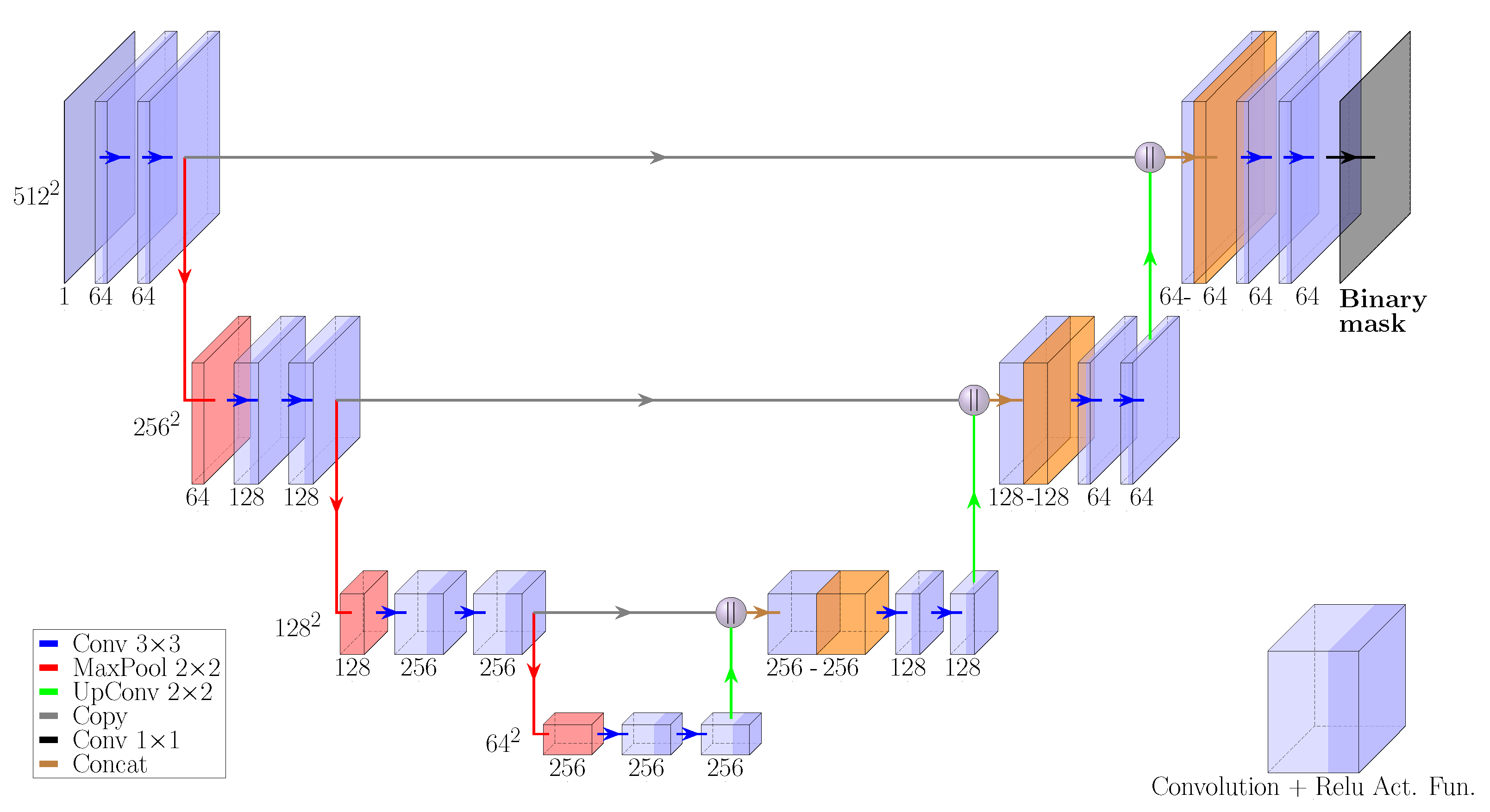
The U-Net is a fully convolutional neural network (FCN) which was first used for segmentation of biomedical images and was later adapted to space-based applications such as crater detection [28]. The network architecture in this paper is chosen to be a slightly modified version of the original one as shown in Figure 1, and it has a symmetric encoder–decoder structure: the encoding, downsampling path is a stacked sequence of two ReLU convolutional layers followed by a max pooling layer. At each level, the number of filters doubles, reaching its maximum value at the bottom.
The decoding upsampling path contains up-convolutional layers concatenated with layers coming from the corresponding downsampling level in order to preserve already learned features. The concatenated layers are followed by dropout and a sequence of two convolutional layers up to the output layer in which a final sigmoid-activated convolution produces data ready to be binarized. The present U-Net will be fed with images and their corresponding masks.
Configuration parameters used for this network to prevent overfitting are as follows:
- Learning Rate: It is an optimizer’s parameter that fixes the step size at each iteration during minimization of the loss function.
- Regularization Factor: It is a parameter needed for the l2 regularization based on penalization of the cost function.
- Dropout Rate: It regulates the percentage of inactive network elements in the dropout layers during training and the validation process.
- Kernel initializer: It sets the weight initialization method; in this case, it is set on he_normal [30].
In this work, Adam was chosen as the optimizer and Binary Crossentropy was chosen as the loss function.
2.3. Dataset Creation and Input Data Preprocessing
The dataset created and used for the U-Net training phase is provided at [31]. It is composed of 5600 squared monochromatic jpeg images and 5600 associated jpeg masks. All of them have a size of px and a bit depth of 8. Masks’ pixels can have one of two possible values: 0 for background and 255 for foreground pixels.
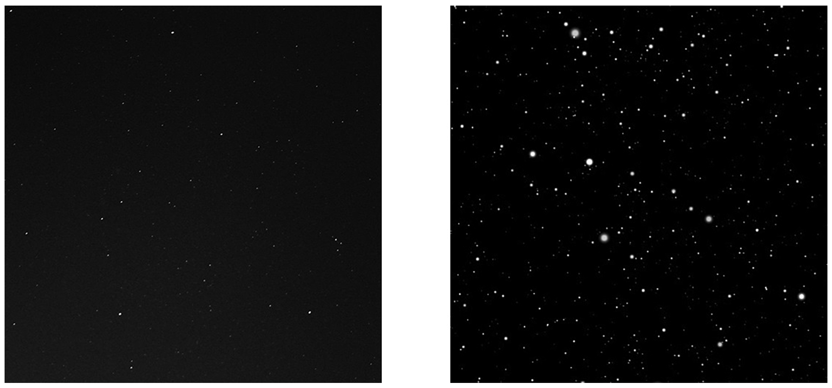
The samples for the training and validation phases are the first 5300 ones. They are generated from a batch of 600 images to which 180° clockwise rotation, 90° clockwise rotation, added noise, increased stray light, blur effects, increased luminosity, contrast and further modifications have been applied. This original batch is made of 300 samples coming from several night sky acquisition campaigns and 300 samples randomly acquired using Stellarium [32] software in night sky conditions considering different FOV and attitudes (Figure 2). Acquisition campaigns were performed using several kinds of cameras and objectives: ZWO ASI 120MM-S camera with default optics, reflex Nikon D3100 equipped with a Nikkor 18-105 mm and a ProLine PL16803 camera coupled with an Officina Stellare RiFast 400 telescope.
Last 300 dataset images were obtained with a high fidelity star tracker image simulator (HFSTIS). It is used to simulate realistic night sky images, simulating all the physical, functional and geometrical characteristics of the star sensor, along with all the instrumental and environmental noises [33,34,35,36,37]. Simulator images were used only in the test phase to provide independent samples the network has never been trained on to monitor the generalization capability of the trained network.
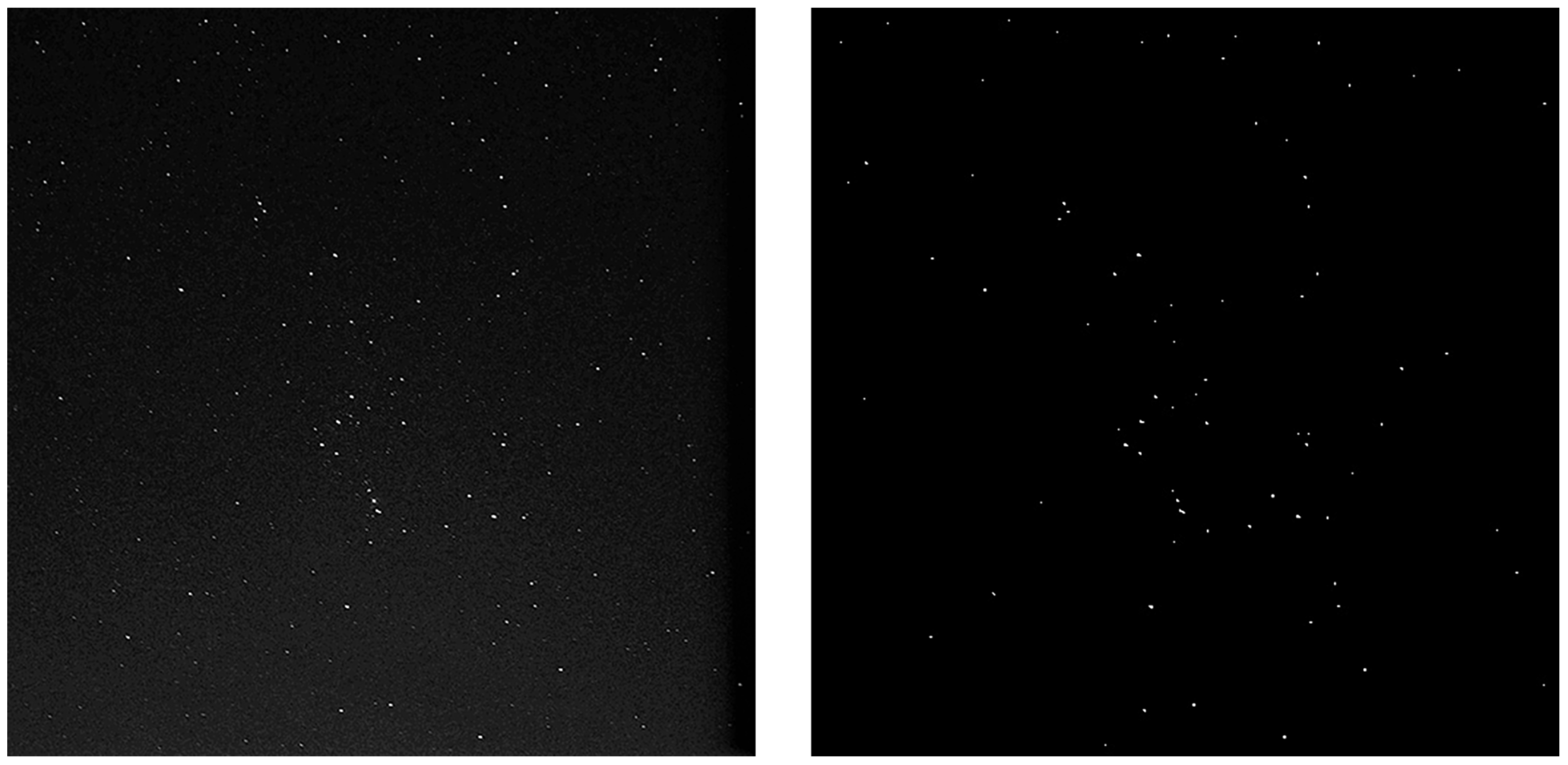
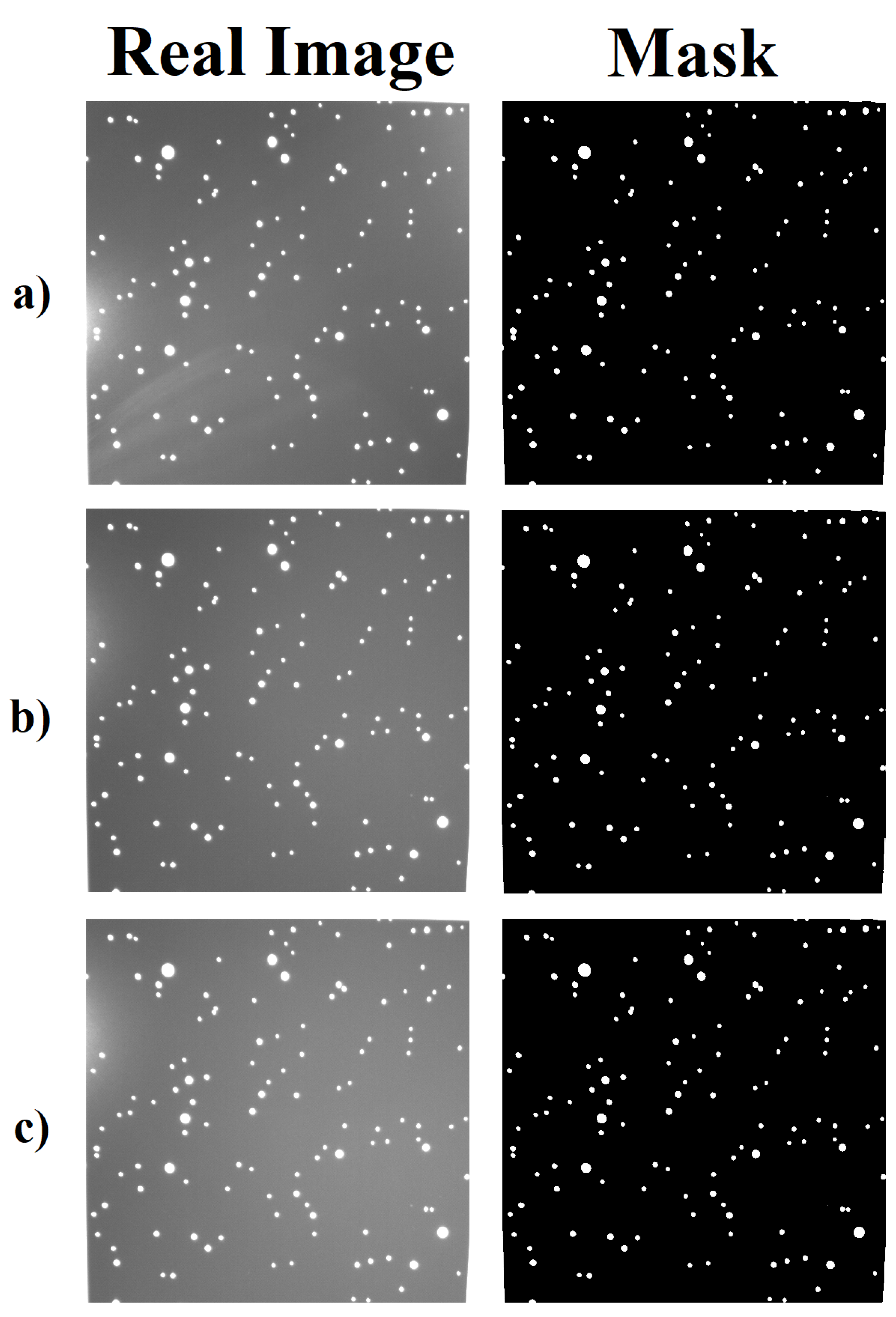
The dataset contains images of night sky where stars are the main actors but where planets, light pollution caused stray light noise, SEUs, clouds, airplanes’ streaks, satellites, comets, nebulae and galaxies appear as well. Masks were obtained using specific thresholds for different groups of images from different campaigns, sensors and software. In particular, mask creation was carried out using Adobe Photoshop CC 2019 with the scope of obtaining just the most salient objects in the FOV and filtering all the noise and undesired objects cited above. An example of a dataset image and mask is provided in Figure 3, where it is clearly visible that just the brightest points appear inside the mask. Input images and mask preprocessing is performed in order to organize these data in two float 4D tensors for NN training and testing. Every image is converted into floating point arrays and normalized using its maximum value to carry out an image adaptive normalization process; every most significant image pixel will have an associated value close to 1. This will help the network detect the most significant pixels and make the learning process easier for the net by constraining the interval of signal values between 0 and 1. Moreover, this normalization process improves the algorithm capability of working with images that have different range of energy levels. The same process applies for mask data vectorization and normalization, with the only difference being that the normalizing factor is constant and equal to 255 for every mask.
It must be pointed out that the dataset does not contain only point-like stars but also even images where they appear as streaks due to the angular speed of the sensor. Considered angular speeds are within the [,]. This allows the proposed AI-based algorithm to work properly even in situations where the star sensor is rotating with respect to the fixed stars or where a sidereal pointing of the camera occurs together with RSO passages.
Concerning the noise, 5300 images for training and validation are generated from a batch of 300 images. This batch is composed of several acquisitions performed with different sensors and so, different noise conditions. In less-noise-corrupted images, an added source of uniform noise was added using Adobe Photoshop 2019 (Filter->Noise->Add Noise->Uniform 6.3%). For different stray light conditions, +0.5, +1 and +1.5 stop in image exposure were added randomly. It is quite impossible to retrieve the sensors’ noise level characterization due to the different kind of sensor used and the unavailability of their noise features. For the last 300 test images, it is possible to characterize the noise:
- Shot Noise: Poisson probability model and proportional to square root of the detected signal;
- ReadOut Noise (RON): Normal distribution with mean 0 and standard deviation of 82 ;
- Dark Current (DC): Constant value of 550 ;
- Dark Signal Non-Uniformity (DSNU): Normal distribution with 1 mean value and a standard deviation of 0.065;
- Photo Response Non-Uniformity (PRNU): Normal distribution with 1 mean value and a standard deviation of 0.01;
- Stray Light: 30000 .
2.4. Algorithm Design and Configuration
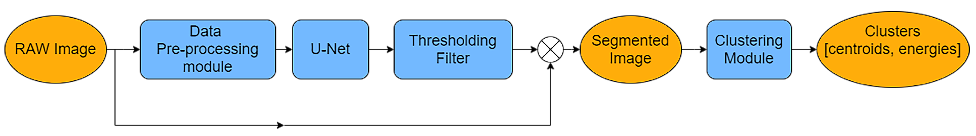
In this section, our proposed AI-based algorithm’s scheme is described and shown (Figure 4). It will be referred to it as the brightest objects sky segmentation (BOSS) algorithm.
The monochromatic raw image from the camera arrives at the preprocessing module where it will be resized, normalized and vectorized into a floating point array. This module will be tailored according to specific sensors’ bit depth, while the size must be the one the NN is trained on. Then, the array is processed by the trained U-Net which gives its output prediction. This is a 2D array where every pixel has an associated value of probability p of being foreground. If then this value is rounded up to 1. After the thresholding filter, a binary image is obtained, and its element product with the original image will provide an array with just active pixels’ energy values. This output will be used by the clustering algorithm to detect clusters and compute their centroids and total energies. The clustering module developed within this work takes all the active pixels in the segmented image and organizes them in a list. Then. it associates the first pixel in the list to the first cluster and starts to verify if the next pixels are part of the same cluster or not through a distance-based criterion. Whenever the next active pixel does not belong to the already identified clusters, then a new cluster is identified.
The distance criterion uses the Euclidean norm and the condition to assess the membership of two active pixels ( and ) to the same cluster as expressed by Equation (1).
The clustering algorithm then first performs a filtering action with a minimum and maximum dimension and then a sorting of all the clusters. A minimum dimension filter is needed to avoid a possible noise signal in the clustering outputs (ex. hot pixels), while the maximum dimension filter is needed to avoid great detected clusters due to non-stars objects.
The sorting operation is then performed in descending order and considers the first N clusters in output from the previous filtering actions. It is based on a combination (Equation (2)) of the clusters’ dimension (), energy () and maximum energy value () over the cluster because this sorting index proved to be suitable to select the best clusters for star pattern recognition purposes with the conducted tests.
N is computed by applying a 1.25 factor to the average number of stars which depends on the FOV and cut-off magnitude of the selected sensor [2]. The maximum number of clusters in output is fixed a priori to process just the most significant ones, and the 25% margin factor is selected to take into account possible uncertainties of the average number of stars formula.
The U-Net is capable of resolving background and foreground pixels after training, validation and test phases, but it still gives continuous values that have to be discretized. This is the reason why the thresholding filter and the selection of a reasonable value for will be described in the next sections in order to obtain the best correspondence between algorithm prediction and targeted masks. Once the U-Net is trained and selected, the BOSS algorithm will be compared with traditional image segmentation ones, both described in the next section in terms of segmentation performance.
2.5. Traditional Image Processing Algorithms Description
In this framework, several traditional algorithms for image segmentation were selected for comparison with the AI-based proposed algorithm. In the following, five algorithms are considered. They are based on Niblack’s method, Otsu’s method, the weighted iterative threshold approach (WIT) [1] and two local threshold (LT) approaches.
2.5.1. Niblack’s Algorithm
Niblack’s method is based on the computation of a threshold value T which is a function of the energy mean value and standard deviation computed over a rectangular window. Through its sliding over the whole image, it is possible to then identify which are the foreground and background pixels by comparing the window’s pixels energy values with the local threshold.
where k is a parameter which varies between −0.2 and −0.1, while the other parameter is the dimension of the window (supposed squared in our paper with side ).
2.5.2. Otsu’s Method
It is based on the gray level image’s histogram. It aims to find the threshold value which minimizes the intraclass variance [38] of the thresholded black and white pixels. The main advantage of this method is its unparametric nature which avoids the need for configuring it according to the image noise level.
2.5.3. Weighted Iterative Threshold Approach
This method is an iterative way to compute the optimal threshold for a given image. At each step, the threshold is computed using the following formula:
where and are, respectively, the average gray level values of foreground and background pixels. With this new threshold, new sets of foreground and background pixels can be computed with the following mean values, and the process repeats with the computation of a new threshold. When the difference between two successive thresholds is lower than a certain tolerance , the process stops. This algorithm is dependent on a scalar parameter which can vary in the range .
2.5.4. Local Threshold Approach Based on Rectangular Areas (LTA)
The algorithm used is from MATLAB. It scans the whole image and computes a local threshold. The used size of the window is given by the following formula:
Over this window, a Bradley’s mean [39] is computed. By comparison between a pixel’s energy value and this local mean, the classification of the pixel as background or foreground occurs. This process is carried out using a scalar parameter called sensitivity (S). It varies in the range [0, 1] and indicates sensitivity towards thresholding more pixels as foreground.
2.5.5. Local Threshold Approach Based on a Moving Streak Average (LTS)
The last one, the segmentation algorithm [40], can be configured using a static or a dynamic approach [41] for the background noise estimation [38]. In this work, a dynamic approach based on a zigzag local thresholding with moving average is used [42]. In particular, a pixel is saved if its energy value is greater than the background noise, evaluated through a moving average line-by-line, plus a threshold .
The information relative to the segmented image is used for the clustering process, i.e., the combination of segments belonging to the same star streak [34,35,36,37]. The most important step required by the clustering algorithm is the evaluation of the primitive clusters containing pixels which share at least one corner. A suitable technique has been developed in order to relate streaks in the image to the same star if the corresponding streak is broken into multiple streaks due, for example, to the high rate of the spacecraft. Three conditions will be satisfied related to the minimum distance, the direction and the density of the considered primitive clusters. Centroids’ coordinates of each cluster are evaluated, taking into account the energies of segments merged to build the cluster itself according to Equation (6):
where are the baricenter coordinates of the j-th segment in the image plane, while is the sum of the energies which forms the cluster i-th:
2.6. Comparison Indices
The performance comparison between the BOSS algorithm and other algorithms will be detailed in the Results section. The compared algorithms will be tested with a set of gray scale images and relative masks; in order to assess the accuracy of the algorithm’s predictions against test masks, the use of suitable indices is necessary. These indices are heavily used in the segmentation field to compare two image masks as the U-Net output and ground truth from the dataset actually are. These indices can also be used to compare predictions of any couple of segmentation algorithms. Before introducing them, the notion of true positive (TP), false positive (FP) and false negative (FN) must be given:
- TP: A counter that increases by one unit every time both the predicted pixel and the reference one belong to the foreground set;
- FP: A counter that increases by one unit every time the predicted pixel belongs to the foreground set while the corresponding mask one is a background pixel;
- FN: A counter that increases by one unit every time the predicted pixel belongs to the background set while the corresponding mask one is a foreground pixel.
A good prediction has background pixels and foreground ones almost in the same position inside an array as the associated ground truth mask. The goodness of the prediction can be assessed through the evaluation of Precision, Recall and F1 index.
It represents the percentage of the TP with respect to the sum of TP and FP. The lower the FP is, the higher the Precision will be (with maximum value equal to under ideal conditions).
It represents the percentage of the TP with respect to the sum of TP and FN. The lower FN is, the higher the Recall is (with maximum value equal to under ideal conditions). Recall and Precision are similar but with a slight difference. This is due to the distinction of FP and FN. Every time an FP or FN occurs, there is a discrepancy between the prediction and the reference mask, but the difference between FP and FN helps us better understand the behaviour of the trained network.
Another index to be defined is F1:
This index combines the Precision and Recall and lets us understand when the best compromise between FP and FN occurs. It reaches its maximum value when the discrepancy between the prediction and the mask is minimized. Ideally, the maximum value of F1 is 100%, but the best prediction will be the one with the highest value of the F1 index.
3. Results
In this section, results of U-Net’s training, validation and testing will be shown, together with a reasonable choice for and number of initial filters. Then, a comparison test of the BOSS algorithm with traditional ones is conducted against the same set of images.
3.1. U-Net Training and Test
The U-Net tested here is configured with the values shown in Table 1.
Training and validation were performed in Tensorflow Keras [43] considering three epochs and a dimension of the training batch equal to three. This has been conducted for four different values of initial filters: 16, 32, 64 and 128. This choice was made to see how performance in terms of accuracy and loss varies with the increasing network complexity in order to select the minimum required number of filters while achieving satisfactory performance. Every trained network reached accuracies higher than 99.80% after the first epoch and remained constant for training, validation and testing. The same behavior applies for the final losses which are not higher than 0.016. Moreover, no overfitting phenomenon was indicated.
The training, validation and tests were performed on the following workstation:
- CPU: AMD Ryzen Threadripper PRO 3975WX 32 Cores 3.50 GHz
- RAM: 128 GB
- GPU: Nvidia Quadro RTX 5000.
3.2. Tuning of Thresholding Filter
From the previous phase, it seems that every model has learned its task, but their output is not yet a binary mask. To achieve this, a thresholding operation has to be performed to select a suitable value of . Its tuning is conducted in a range of values from 0.01 to 0.9 and different models over the 300 images test set.
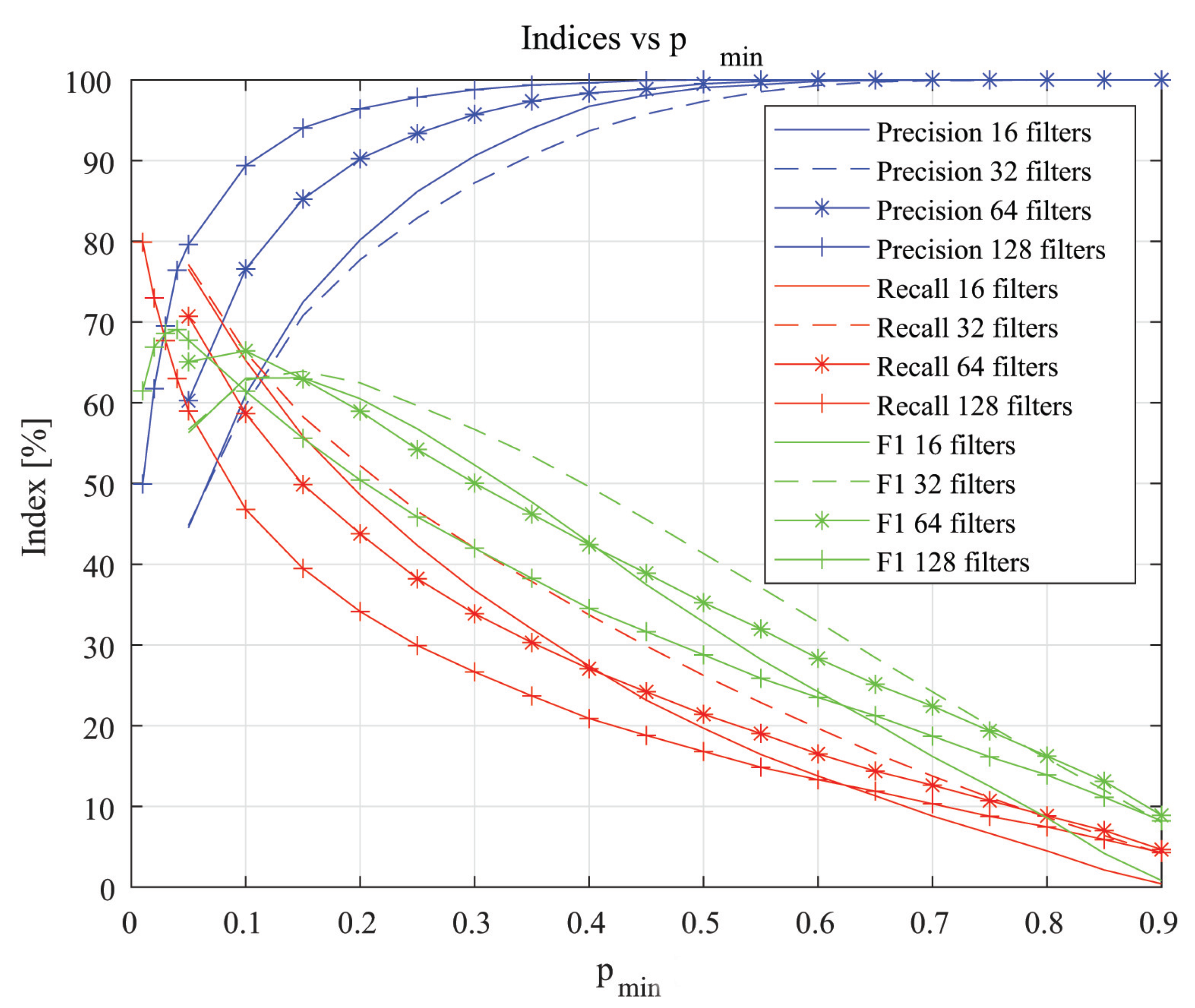
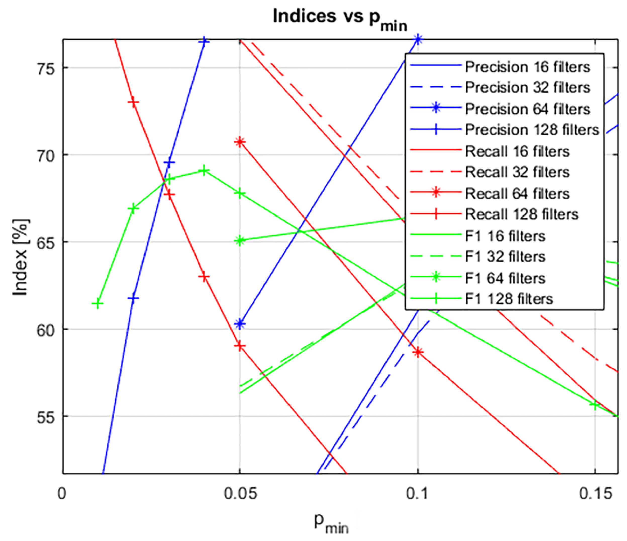
For every and model, the values (over the whole test set) of Precision, Recall and F1 are computed and reported in Figure 5. It can be seen (Figure 6) that the network with 128 filters performs better in terms of output mask. The value around 69% for the F1 index means a minimized number of discrepancies between the BOSS algorithm’s prediction and the mask. This value is the highest one if the best achieved F1 values are considered among all the networks. Because of this, a model with 128 filters and was chosen for the BOSS algorithm design.
Precision behaviour for low values is due to an increasing number of FPs because as the decreases, the number of FPs becomes greater if compared to TPs. For higher , the number of FPs tends to 0, while TPs tend to a finite value, and the Precision is achieved. This maximum value of Precision still does not mean that the prediction is good.
A similar discussion can be conducted for the Recall: as the decreases, the risk of predicting FNs decreases with respect to TPs. This is why Recall grows. For higher , the increasing number of FNs causes the Recall value to fall towards .
A test with a 256 initial filters model was conducted, but performances do not show relevant improvements with respect to the 128 initial filters model, while the required storage memory and computational time increment is not negligible (and also undesired). This is the reason why they are not reported in Figure 5.
3.3. BOSS Algorithm Tests
In this section, examples of BOSS algorithm applications for stray light removal and ghost noise removal in night sky images are shown. The aim of a good segmentation in this case is to retrieve the point-like stars and streaks (RSOs) while removing background pixels that are often badly affected by several noise sources. By noise, we mean that part of the image signal that does not represent the target scene and must be filtered in a certain way. It corrupts the image actors, and if the ratio between the useful signal and noise is higher than but close enough to one, the useful signal could be filtered out as noise and lost for further processing. The image noise is due to several causes briefly divided into the following:
- Inner noise: It is due to the sensor components, electronics and realization technique.
- External noise: It is due to planets, the Sun, the Moon, the Earth, hosting platform structures and camera baffle together with lenses non-uniform reflection.
3.3.1. Sidereal Pointing Camera and Different Exposure Times
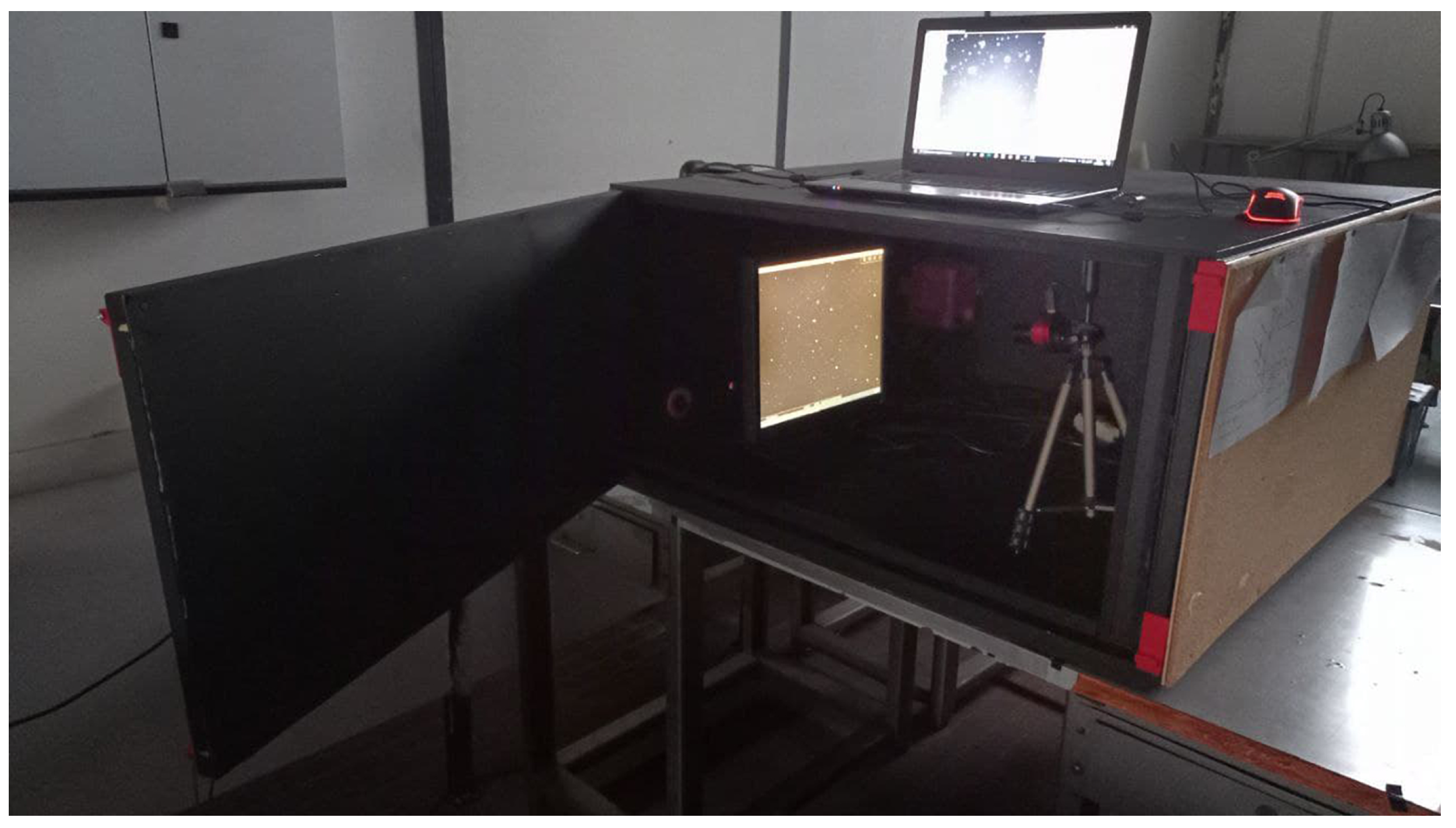
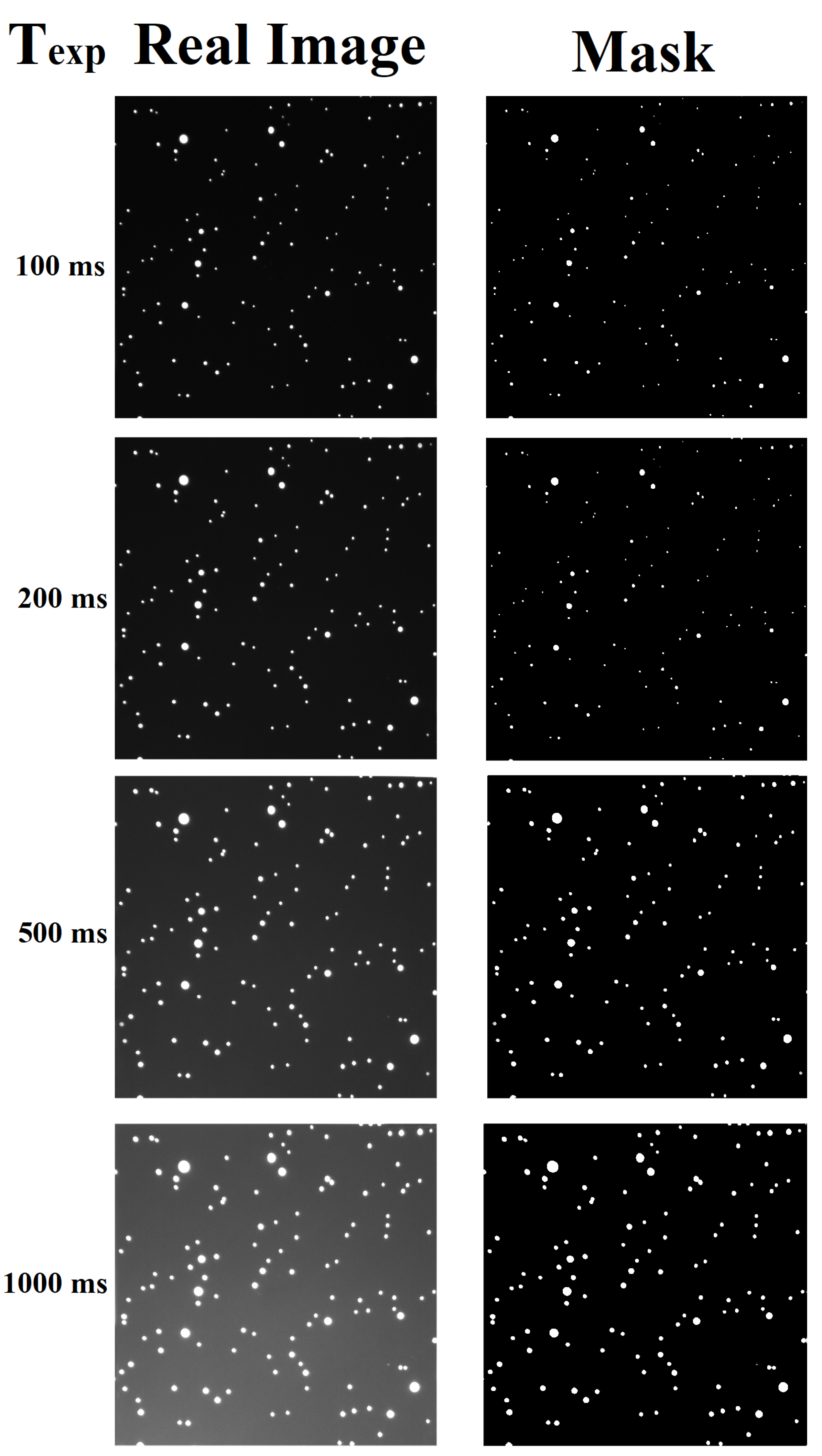
This test aims to investigate the BOSS algorithm behaviour against an increasing stray light noise source. Stray light noise is due to external light sources which cause a flare all over the image. It can be experienced when an optical-space-based sensor has a boresight direction close to the Sun, the Moon, or another high luminosity source. This stray light can have a uniform intensity or uniform gradient. If it is too strong, it can hide the useful signal associated to stars and RSOs and make them difficult or even impossible to be segmented and detected. A change in the stray light intensity during the mission may cause the need for continuous sensor calibration. This could be avoided with a calibration-less algorithm such as the U-Net-based proposal in this work. This noise can increase with the increase of the sensor exposure time as the amount of collected photons proportionally increases with this time interval. In this test, images acquired with a night sky simulator facility (NSSF) (Figure 7) were used. This facility is made of a darkroom where a ZWO ASI 120MM-S camera points towards a screen. Here, Stellarium software is used to simulate the sky as seen by a specific camera with a selected FOV and optics (2.8 mm of focal length, f/1.4). All the simulated stars have a magnitude lower than 6.5 in Figure 8 and Figure 9. With this software and the real camera, it is possible to simulate the working of a camera pointing at the night sky both for stars and RSO segmentation and detection for preliminary results. Images’ noise sources are the real camera noises plus a further stray light source due to the screen technology (backlit screen).
A sidereal pointing was considered in this test just to see the effect of the image stray light noise increasing with the increase of the camera exposure time. Here 100, 200, 500 and 1000 ms of exposure were considered, and the original images and segmented ones are reported below (Figure 8). From this figure, it is possible to assess that the segmentation algorithm removes the stray light and correctly segments the stars. As the noise increases, the foreground pixels increase because of the increasing magnitude of the targets.
3.3.2. Ghost Noise Removal
This test aims to investigate the BOSS algorithm behaviour against a nonuniform gradient noise: ghost noise. This undesired noise source is due to camera lens reflections, spacecraft structure reflection and dust all over the camera lenses. The ghost noise is named in such a way due to its appearance: it is a vague and partially transparent shape superposed on the background and image objects and a nonuniform gradient signal which may cover the whole image or part of it. If it is too strong, it can hide the useful signal associated with stars and RSOs and make them difficult or even impossible to be segmented and detected like the stray light. A change in the ghost noise intensity during the mission may cause the loss of information if no calibration is performed. This could be avoided with a calibration-less algorithm such as the U-Net-based proposal in this work, and it is shown with simulated images in Figure 9 and with real images in the next sections. This noise does not increase with the increase of the sensor exposure time, while the gradient level tends to be more uniform. Here, the same facility has been used but with an added external flashlight source. The stray light and ghost noise were produced with three different positions of an external flashlight source which was moved at different heights on the left side of the camera and target screen inside the darkroom. Even here, it is possible to see a good segmentation quality provided by BOSS (Figure 9). A particular thing that can be noted is the white edges at the images’ corners. They are due to a displayed undesired box in the night sky images made by Stellarium.
3.3.3. Real Image Test on BOSS Algorithm Output
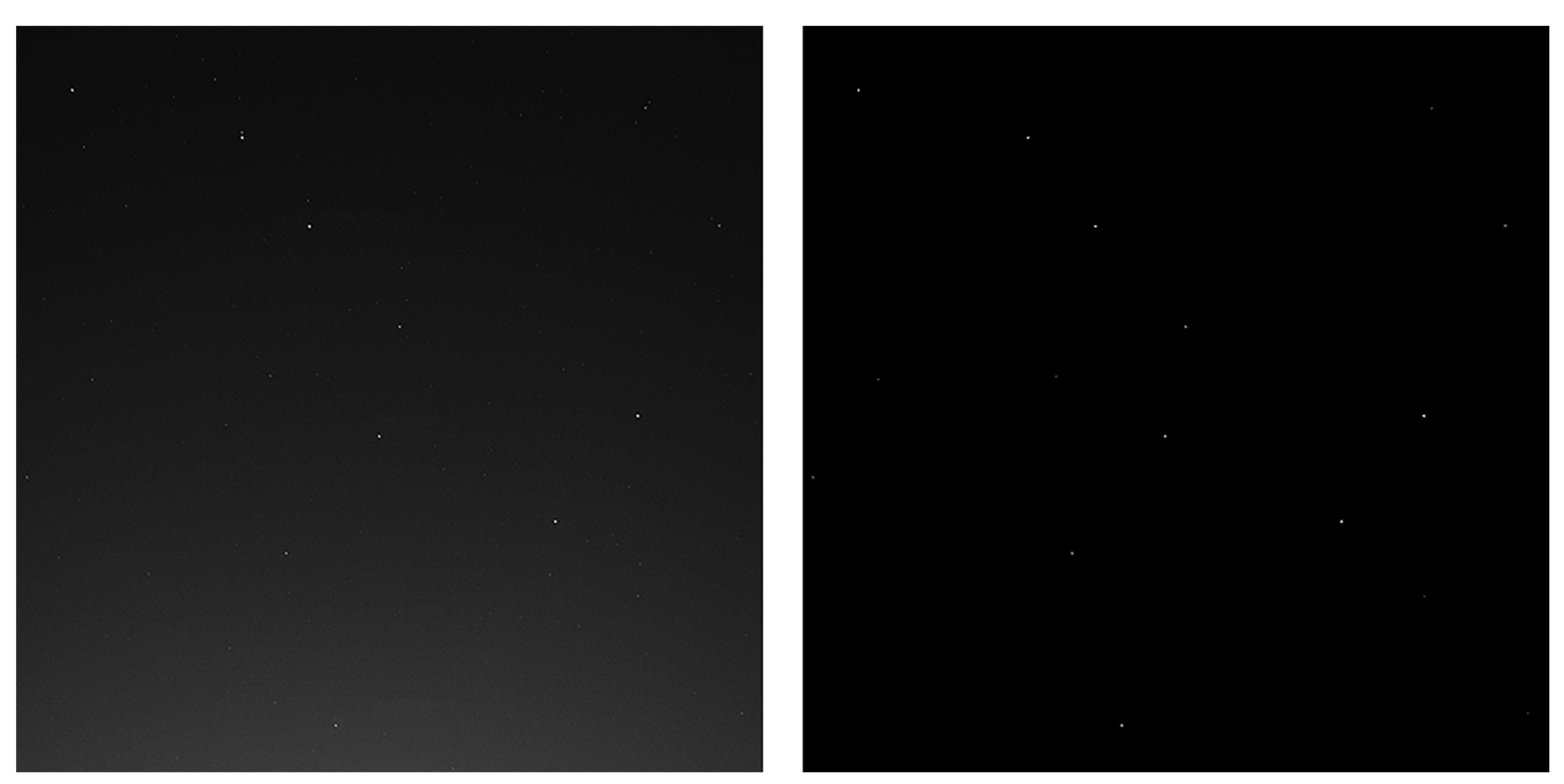
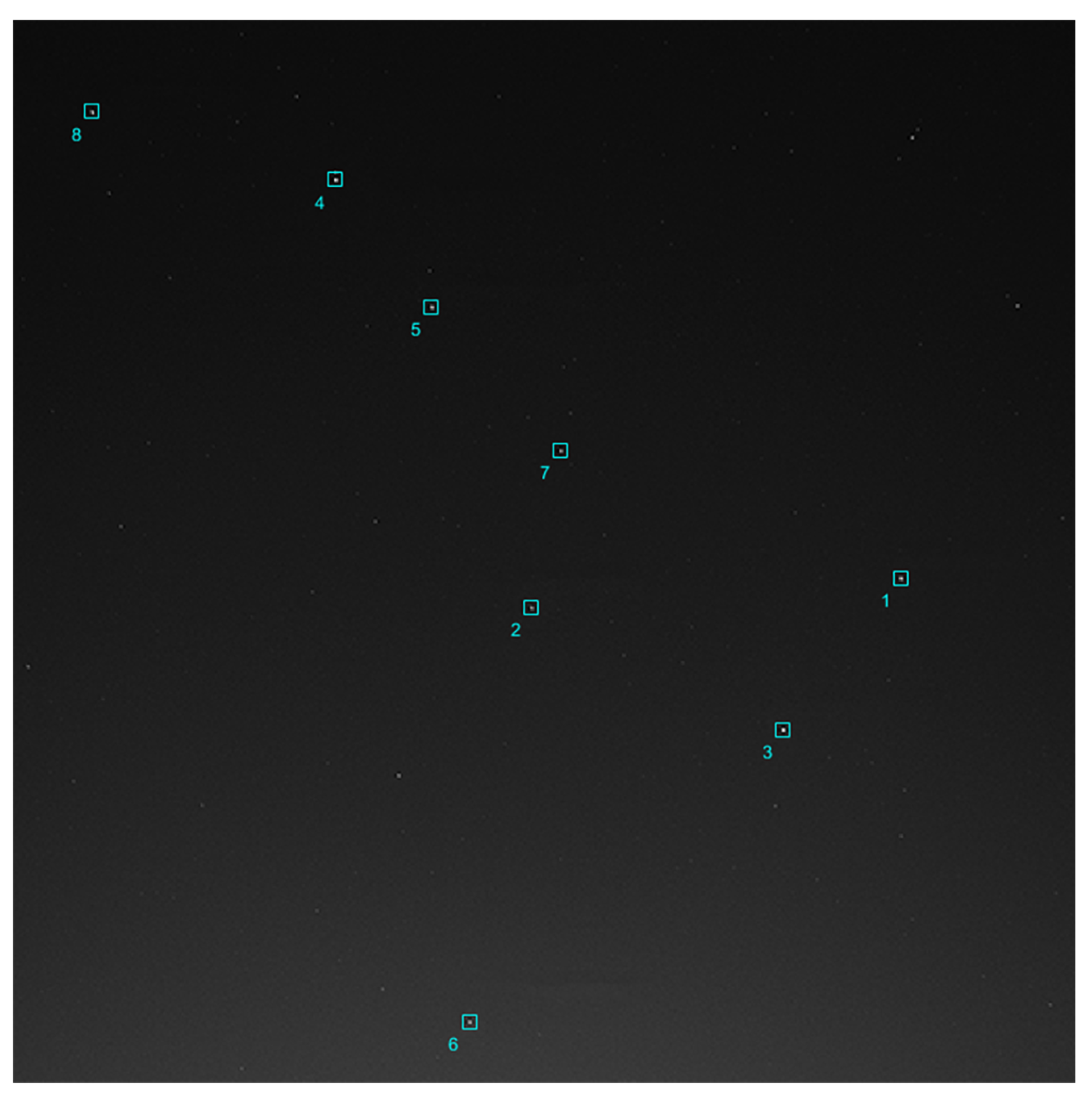
In this section, a real night sky image is considered to test the BOSS algorithm against it. The aim of the test was the demonstration of the BOSS capability of providing a suitable segmentation and stars localization with a real image and real noise sources. The real image is shown in Figure 10 together with the segmented image. The camera used is a Nikon D3100 whose image has been cropped and resized to the U-Net input size of 512 pixels. The image contains, besides real sensor noises due to the electronics, a strong stray light source coming from the bottom and due to nearby city light pollution (Acquisition site: Tusculum/Frascati, Rome, Italy). Parameters of the camera are listed in Table 2. Clustering algorithms extracted the centroids of the eight brightest stars in the FOV and correctly localized them. They are shown in Figure 11.

Table 2.
Nikon D 3100 camera features. The image has been resized to 512 px and 1:1 aspect ratio.
| Feature | Value |
|---|---|
| Size | 512 px |
| Aspect Ratio | 1:1 |
| focal length | 30 mm |
| FOV | 28.79° |
| pixel size | 30.07 m |
| Cut Off Magnitude | 4.0 |
| f-number | f/2.0 |
Figure 10.
Ursa Major constellation segmentation provided by the BOSS algorithm. Left: real Ursa Major image; right: BOSS output of the Ursa Major real image.
Figure 10.
Ursa Major constellation segmentation provided by the BOSS algorithm. Left: real Ursa Major image; right: BOSS output of the Ursa Major real image.

Figure 11.
Ursa Major constellation stars localization performed by the BOSS algorithm. Names and visual magnitudes of the segmented objects have been reported in Table 3.
Figure 11.
Ursa Major constellation stars localization performed by the BOSS algorithm. Names and visual magnitudes of the segmented objects have been reported in Table 3.

Table 3.
IDs, names and visual magnitudes of the segmented objects in Figure 11.
Table 3.
IDs, names and visual magnitudes of the segmented objects in Figure 11.
| ID | Name | Magnitude |
|---|---|---|
| 1 | Dubhe | 1.95 |
| 2 | Phecda | 2.42 |
| 3 | Merak | 2.34 |
| 4 | Mizar | 2.25 |
| 5 | Alioth | 1.75 |
| 6 | Psi Ursae Majoris | 3.16 |
| 7 | Megrez | 3.33 |
| 8 | Alkaid | 1.80 |
3.4. BOSS Algorithm Comparison with Traditional Image Segmentation Algorithms
Here, a comparison between BOSS and traditional algorithms is conducted. The F1 index (Equation (10)) is chosen to compare the performance of the algorithms. Every algorithm was tested against the same test set of 300 simulated images [31]. Otsu’s algorithm did not need to be configured, while LTA, WIT and LTS algorithms did. For these configurable algorithms, a tuning of their parameters was performed, and the F1 index was computed for every combination of their internal parameter.
3.4.1. Algorithms Comparison Procedure
The rationale behind the algorithm comparison is described in this section. The comparison dataset was composed of 300 images and 300 reference masks. Each reference mask represented the desired result of the segmentation process. Every reference mask was manually obtained using Adobe Photoshop 2019 (Image->Adjustments->Threshold), selecting a suitable threshold level because of the varying noise conditions over the 300-image test set.
Now, the scope compared the output of the generic segmentation algorithm with the corresponding reference mask. The procedure was as follows:
- The output mask was compared with the reference mask pixel by pixel;
- The number of FP, FN and TP were updated during the mask comparison;
- FP, FN and TP values were used to compute the Precision, Recall and F1 values (these indices were described in the previous Section 2.6 Comparison Indices).
This process was repeated for all the 300 images, and a final averaged value for the F1 index was obtained for the considered algorithm.
This procedure was directly applied for the BOSS and Otsu algorithms because they do not need to be configured: Otsu does not need any configuration parameter, and the BOSS algorithm has its fixed value of which was frozen during its design in Section 3.2.
Niblack, LTA, WIT and LTS require an additional step before computing the final F1 value: the configuration parameters’ optimization. Indeed all of them have at least one configuration parameter to be selected with a suitable criterion:
- Niblack’s configuration parameters are k and ;
- LTA’s configuration parameter is the Sensitivity;
- WIT’s configuration parameter is ;
- LTS’s configuration parameters are and .
By considering the generic configurable algorithm, the averaged F1 index was computed for every combination of the configuration parameters varying in their specific ranges. Indeed, every selected value for the configuration parameter brings the algorithm to be more or less severe in terms of segmentation performance and changes the final F1 index value. Results of this process, using commonly used values for the parameters, have been collected for each configurable algorithm in Table 4, Table 5, Table 6 and Table 7. In the end, the six averaged F1 values for Otsu, BOSS and the optimized algorithms can be obtained and were reported in Table 8.
In these tables, the configuration parameters which maximize the F1 index were considered, and the maximum value of F1 is then reported in Table 8 for the final comparison. In this way, every configurable algorithm was optimized against the 300-image test set in order to make the comparison more challenging for the BOSS algorithm.
3.4.2. Comparison Results
Otsu’s algorithms is the only traditional one which does not need any configuration of parameters. Its F1 score is 0.07%.
The best achieved F1 values for every algorithm are summarized in Table 8 for a fast comparison.
From previous tables, it can be seen that the best F1 score was achieved by the LTA algorithm followed by the LTS one and the BOSS algorithm. Niblack and Otsu behaved worse than the others, while the WIT achieved high but not satisfying performances.
Both LTA and LTS behave better on the test set if compared to the BOSS algorithm. As a first impression, it would seem that the use of BOSS algorithm does not bring any advantage. However, the performances achieved by LTA and LTS were obtained via a tuning of their parameters, while the BOSS algorithm was not tuned after its design. LTA and LTS have to be calibrated every time the noise level changes inside the selected scenario to achieve the best segmentation quality output, while the BOSS algorithm does not need this calibration because it has been trained to segment well with several SN levels. This consideration means that the 69% of F1 index is a generalized performance value, while the 79% and 72% values for the traditional algorithms are optimized and not generalized. LTA and LTS were tuned against the test set, while the BOSS did not need any tuning.
This would mean that a star tracker based on the BOSS algorithm would not require any calibration or segmentation performance degradation during its lifetime in orbit. Even if the sensor’s noise increases with the increasing of the lifetime, the U-Net would be able to adapt itself to several levels of SN ratio because it has been trained to do so. A stray light or a higher radiative region would not affect the quality of the segmentation product very much. With this consideration, the strength and meaning of the BOSS performance can be more appreciated and understood.
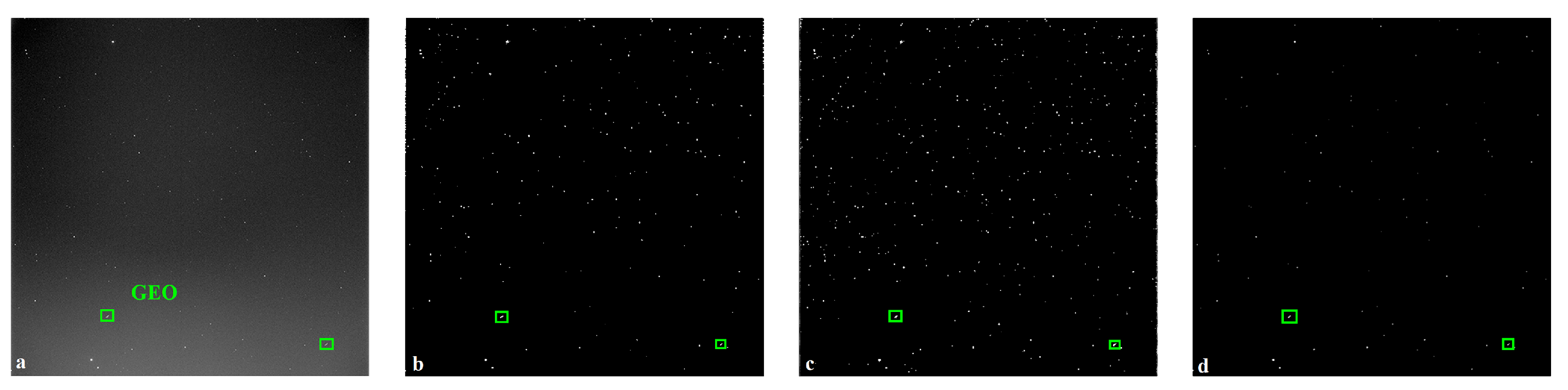
In Figure 12, Figure 13 and Figure 14, it is possible to visually compare the segmentation algorithms output quality of these LT approaches and the BOSS algorithm to understand the limit of a traditional parameterized segmentation algorithm. Three real images of the night sky both from Earth and space were considered with different kinds and levels of noises. A discussion follows for each of them.
Considering the processing of these three figures:
- Figure 12: In the real image, two geostationary satellites (green boxes) on the bottom part of the image are clearly visible with the surrounding star field. This image was obtained via the telescope of the Italian Space Agency Matera Observatory. The noise that mostly appears in this image is a nonuniform flare all over the image stronger in the bottom part and weaker in the top. It is due both to telescope lenses and nearby city light pollution. It is an example of ghost noise. The noise sources associated with the sensor electronics are negligible due to the sensor cooling system which was keeping the camera at −20 °C. There are foreground horizontal and short streaks on the top left and top right edges of the image produced by the LTA algorithm. Moreover, there is some noise that has not been filtered in the whole image, together with the brightest and weakest objects. The same problem is present in LTS’ prediction with a greater percentage of noise. Here, the best output quality is provided by the BOSS algorithm which correctly returns the most salient star-like objects, together with precious RSOs information. All the algorithms return the two small streaks of the geostationary. The stars in the background have a magnitude lower than 12. The used optics is an Officina Stellare RiFast 400 Telescope with a focal length of 1520 mm and an f-number of f/3.8.
- Figure 13: The real image is a detail of a frame from the EBEX mission star camera [44]. The camera is mounted onto a stratospheric balloon carrying a telescope. It is pointed towards the above sky and contains a lot of noise. Indeed, here the dust over the sensor’s lenses, mesosphere wind turbulence and stray light from the Antarctic continent’s albedo are clearly visible and cause a strong ghost noise which covers the few stars in the background. Recognizing stars in this condition is important because star sensors are not used just in space where the absence of atmosphere avoids many noise sources, but also on ships or cruise missiles for navigation purposes, where being able to remove ghost noise due to clouds and other atmospheric effects is mandatory. The LTA (b) algorithm’s prediction shows that few of the brightest stars have been correctly segmented with a not complete filtering action of the noise in the top right part of the image noise. The LTS behaves worst because the strong noise scenario does not allow it to correctly segment the image. There is a lot of noise, with horizontal foreground streaks in addition to the correct segmented stars. This bad behavior is due to the algorithm’s inability to adapt itself to different SN conditions. Here, a re-calibration of the algorithm threshold would provide a better segmentation quality for the mask. In the last image (d), the BOSS algorithm prediction shows the segmentation of all the brightest stars (red boxes) with just a little portion of noise in the most corrupted region. Both the LTA and the BOSS algorithm show some problems with the strong ghost noise conditions but in different regions of the image and in different ways: the BOSS algorithm seems to detect as stars the strong nonuniform brightest corrupted region due to the mesosphere winds in the image, while the LTA seems to have an opposite problem with the darker region in the top right part. The explanation for the BOSS algorithm is that the whitest spots in the ghost noise are recognized as possible embedded foreground objects, while in the LTA case, the gray level gradients in the darker localized region mislead the algorithm in properly segmenting the image. Among the two false positives cases, this LTA behaviour could greatly affect the output mask quality because the gradient in the darker region of the image (generally the 99% of these samples) increases the percentage of noise in the output mask (with possible negative effects both for attitude determination routines and RSO detection).
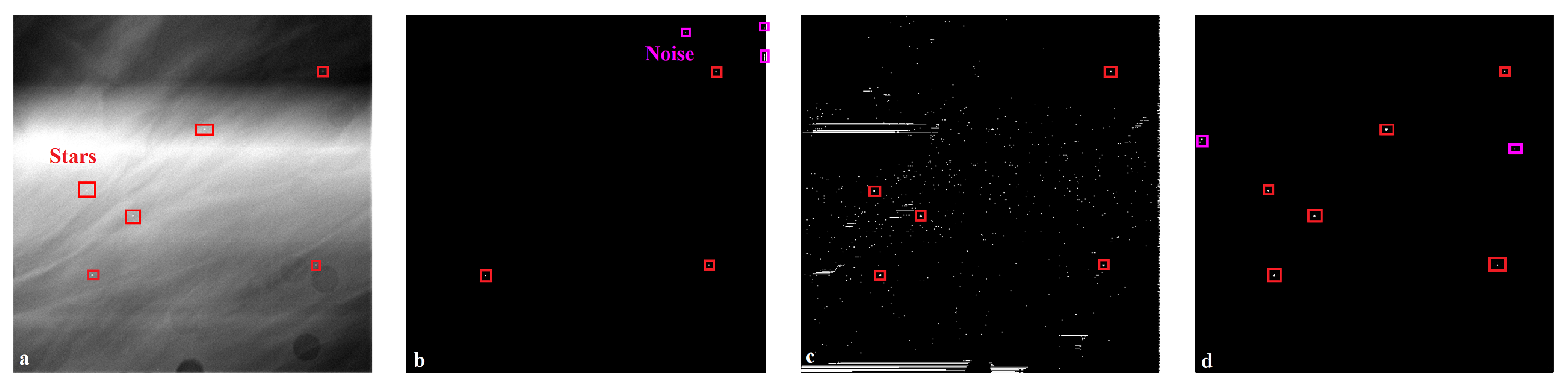
- Figure 14: This is a frame from a video [45] from Juno’s Star Reference Unit (SRU) camera. The image contains stars and a huge number of SEU’s crossing the sensor with different impact angles as the Juno spacecraft crosses Jupiter’s high radiation polar regions. SEUs over images are caused by ionizing radiation which hits the sensor pixels. The more perpendicular to the sensor plane the ionizing radiation is, the more point-like the footprint of the high energy particle on the sensor will be. This noise source can be reduced by shielding the electronics properly, but it cannot be removed. In the analysed image, many SEUs cross the sensor due to the high energetic region where the Juno spacecraft is. It is quite difficult to distinguish the white spots nature, but the purpose of this image processing is to show how the weakest elements on the detector (certainly SEUs under spacecraft inertial pointing condition) are removed. By a rapid inspection of the figures, it is possible to assess that LTA and LTS show similar segmentation outputs, and the SEUs which cross the detector almost tangentially are segmented as streaks. They are segmented by the LTA and LTS algorithms, while they are removed by BOSS. This is due to the dataset used to train the U-Net algorithm. The NN learned to detect just the the brightest star-like objects, filtering all the less salient other ones. Here, the weak streaks of the SEU are removed, but this does not mean that all the star-like objects which appear in the BOSS prediction of Figure 14 are stars; they can be that part of SEUs with a high impact angle.
These examples show that the BOSS algorithm has performances that are slightly lower but acceptable and generalized if compared to the calibrated traditional algorithms. Moreover, it has an intrinsic robustness to SEUs which a traditional algorithm does not normally have.
4. Discussion
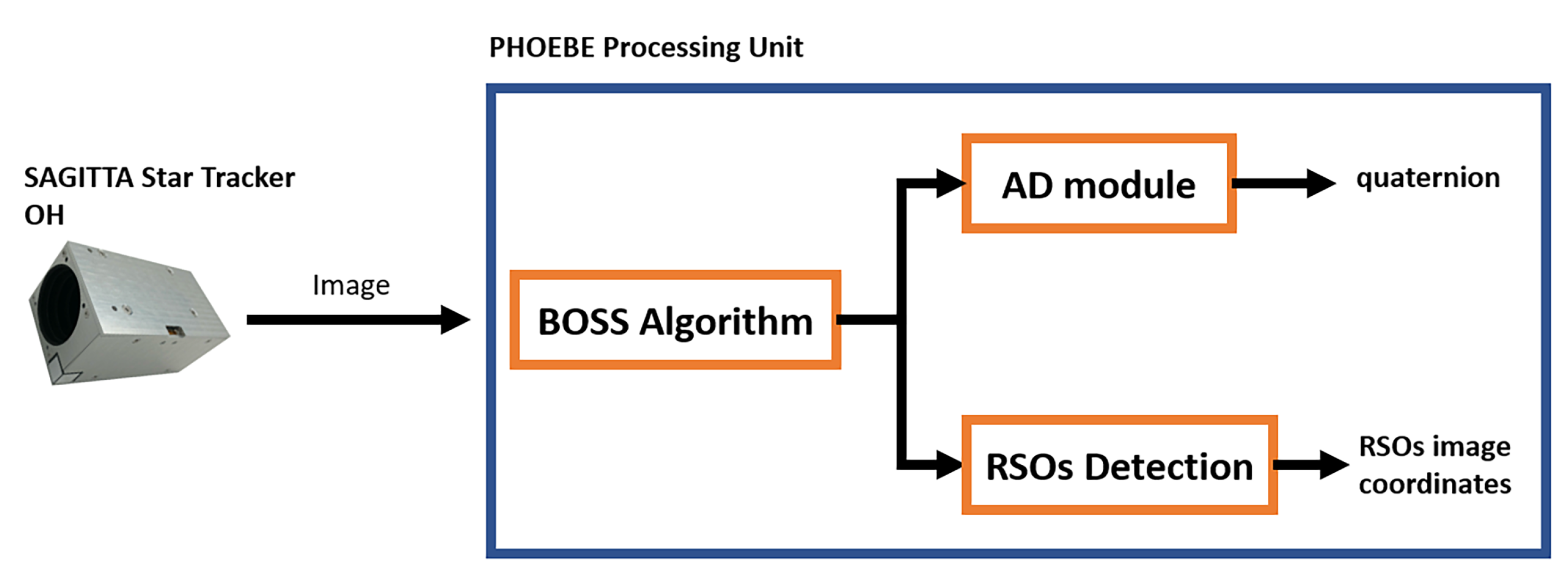
Previous results have proved the high quality of night sky image segmentation provided by the algorithm. The unparametric nature of it makes the calibration operation unnecessary and maintains the high robustness to strong stray light variation scenarios. These features are welcome both for attitude determination and RSO detection through electro-optical sensors such as star sensors. Moreover, the absence of a calibration activity would make an optical camera based on this technology ready to work when the platform is released into its orbit. This algorithm could be used as an image processing main module for lost in space [36] or star tracking routines in common star sensors or RSO detection modules for onboard space surveillance camera or star sensors [40,46]. Both in the former and latter applications, good noise filtering capability is crucial for the success of the star and objects information extraction. This suggests a star sensor based on the U-Net image processing algorithm can be used to validate this technology in a real space mission and increase its technology readiness level (TRL) up to eight. This module will serve both the AD routines and the RSO detection modules. As the image is acquired by the optical head (OH), it is fed into the U-Net-based image segmentation module and then the mask will be used both by lost in space (LIS)/star tracking and RSO detection routines (Figure 15).
The selected components of the payload are the following:
- ARCSEC SPACE Sagitta Star Tracker as OH;
- PHOEBE board as Payload Processing Unit.
4.1. ARCSEC SPACE SAGITTA Star Tracker
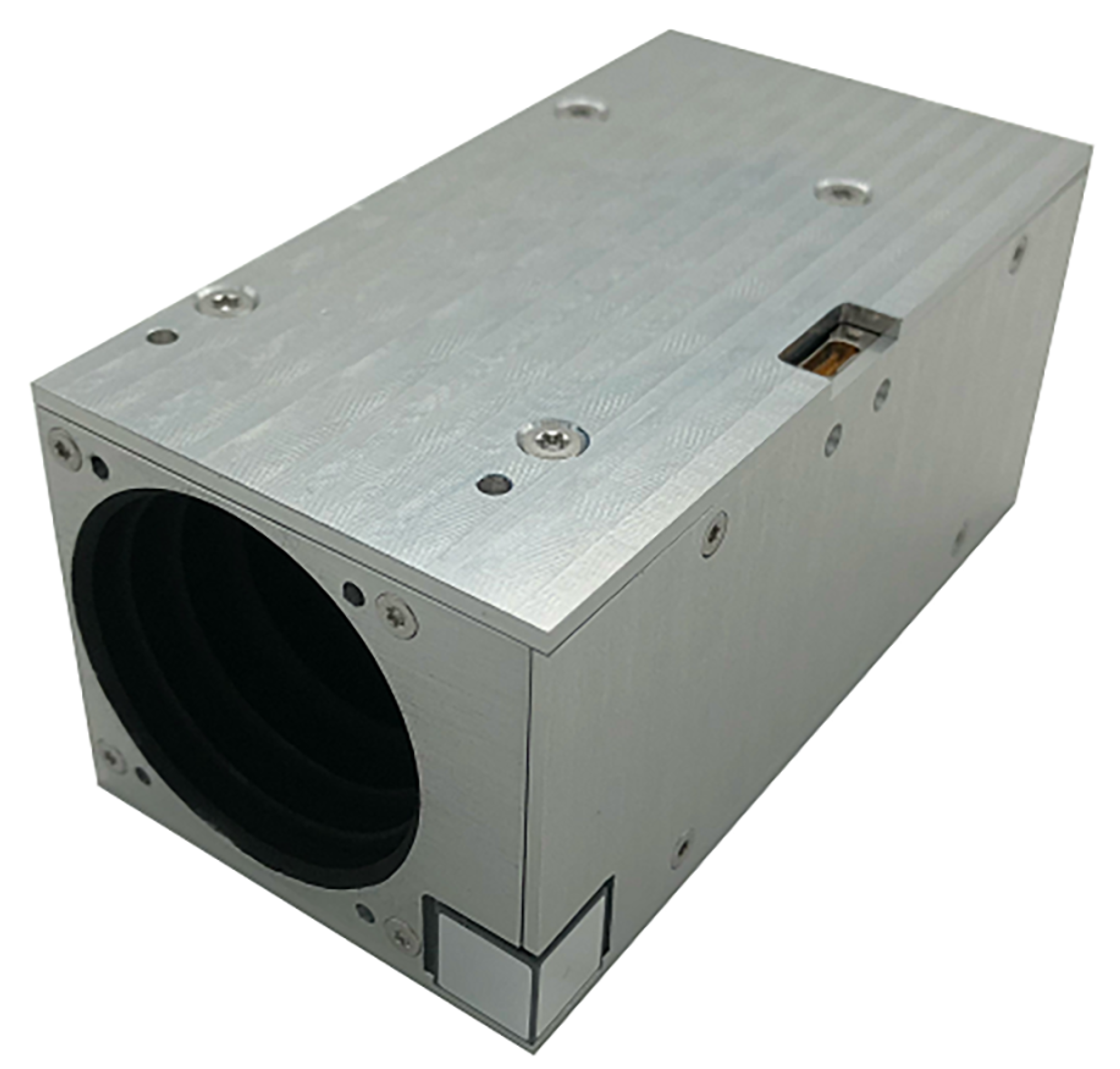
The SAGITTA Star Tracker from ARCSEC SPACE (Figure 16) was chosen due to its good features both for AD and RSO detection purposes. Its most important features for these purposes are the following:
- FOV: 24.8 deg (squared);
- Sensor Size: px
- Cut Off Magnitude: 7;
- Working Frequency: Up to 10 Hz;
- Accuracy: 2 arc seconds (1 sigma) cross-boresight, 10 arc seconds (1 sigma) around boresight.
It is compact and suitable for microsatellites and cubesats missions with dimensions of , a mass of 275 g and a low power consumption of 1.4 W. This device will be customized for the intended missions and used just as OH.
4.2. PHOEBE Board
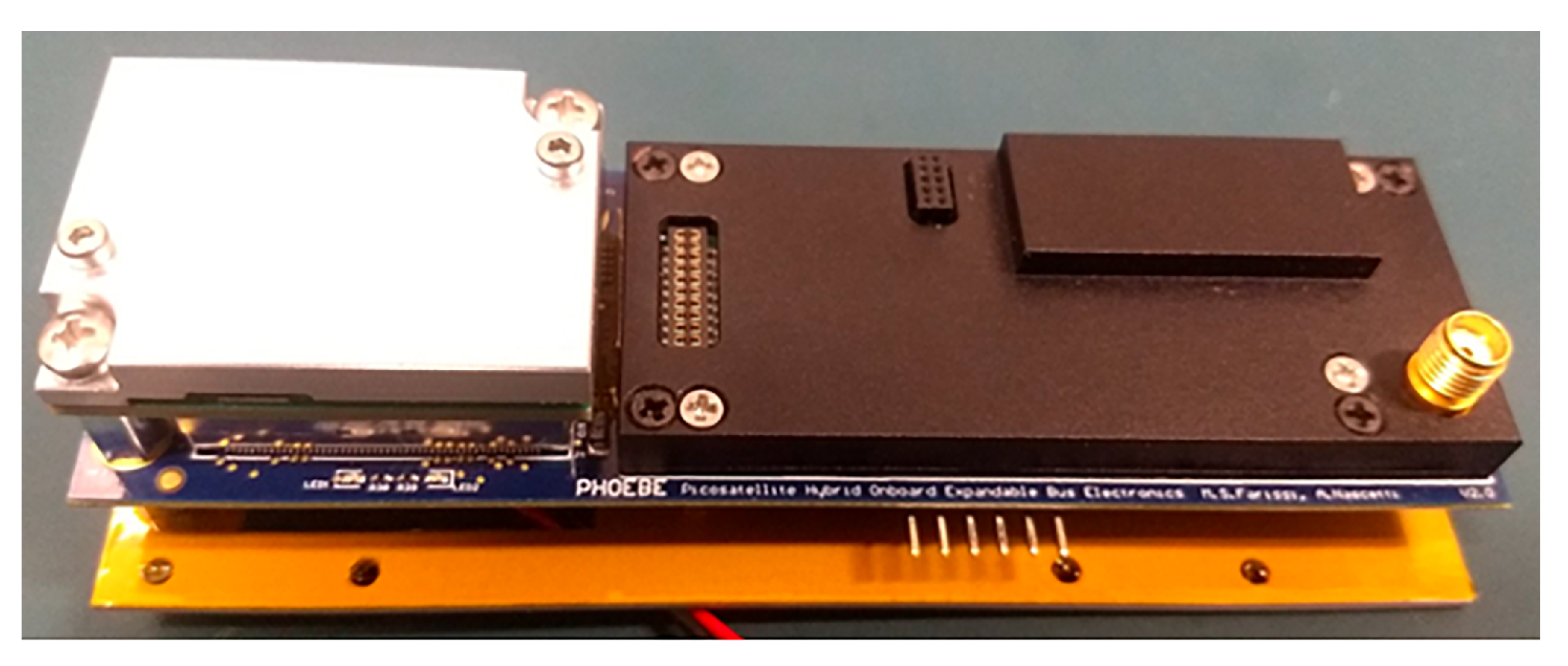
PHOEBE Board [47] (Figure 17) was used by School of Aerospace Engineering, (Sapienza University of Rome) for the STECCO (Space Travelling Egg-Controlled Catadioptric Object) mission. PHOEBE Board Features include the following:
- Microcontroller to handle data and tasks;
- FPGA for fast image data processing;
- Low power consumption: up to 0.3 W;
- Small Satellites Protocol: CAN, and RS485;
- Low Mass: 54 g;
- Dimensions: .
The algorithm will be implemented on the PHOEBE system on Chip/Field Programmable Gate Array (SoC/FPGA) hardware for taking advantage of the parallel computation capabilities of the FPGA which would boost the image processing time and make the proposed algorithm suitable for real-time applications. Indeed, as already demonstrated in another work [48], the SoC/FPGA hardware is able to reduce the processing time by a factor of 70 when compared with a personal computer based solution of the algorithm itself. At the moment, a personal computer processing time of this algorithm requires no more than 5 seconds per image. A materialization on the cited hardware would mean a realistic processing time, not higher than 100 ms, and thus a possibility of working with real 10 Hz star trackers and onboard cameras.
4.3. Small Satellite Mission Proposal
The payload will be able to process camera images up to 10 Hz. This would be good both for AD and RSO detection functions. It will have a total weight not higher than 330 g, a total power consumption not higher than 2 watts with a total volume lower than 0.3 U. It can be installed both on Cubesats and micro satellite platforms, and once in orbit, it can work without any limitations of pointing except for the luminosity conditions: Sun, Moon and Earth to be avoided within the FOV.
- The orbit: The RSOs spatial and mass distribution is strictly related to the former space activities and the collisions and fragmentation of orbiting objects. Several studies have described and modeled the debris evolution during the years, showing that LEO is the most densely populated region around the Earth, especially in 600–800 km altitudes with high inclinations [49]. For this reason, the onboard SST mission will be focused on LEO debris detection at a 600–800 km altitude range, and the orbit selection will be constrained by the sun illumination. To guarantee the correct detection functioning, the optical sensor (on-board camera or star sensor) cannot be oriented against the Sun. Figure 18 shows possible sun-illumination conditions. In particular, represent the target directions, with denoting the observer satellite and one of the debris elements. Satellite cannot detect target because it is backlit, while the sun illumination allows for a correct detection of target by satellite . Another limiting factor to be considered is the presence of the Earth in the FOV, because of the consequent reduced FOV of the optical sensor. To guarantee the visibility of the target by the observer, the vector cannot cross the Earth. Finally, to ensure the same sun-illumination condition during the mission, the best candidate orbits for object detection are the Sun-Synchronous Orbits (SSOs). In particular, the dawn–dusk orbits can ensure a continuous and constant utilization of the optical sensors, while the noon/midnight orbits are not recommended for this kind of application due to the possibility of having eclipses. Due to all these considerations, the selected orbit for the mission will be a circular dawn–dusk SSO with a height of 700 km.
- The purpose: Detection of RSO populations in the LEO region will be with an onboard optical sensor and an AI-based image segmentation routine.
- The Validation: The satellite will be equipped with an attitude control system (ACS) capable of orienting the SAGITTA boresight direction in the along-track direction and anti-Sun direction to maximize the time the RSOs spend inside the FOV. Ground commands will be sent to the platform to schedule the pointing operation to switch between these two targeted directions. An input image will be stored together with the corresponding mask for validation purposes during a test phase. Once on the ground, the raw image will be processed and compared with the onboard produced mask. A match score based on Precision, Recall and F1 indices will be used to assess the correctness of the onboard payload routine. During normal operation, the payload will be responsible for the provision of the attitude for the onboard platform. The platform will be equipped with a reliable and independent attitude determination module to compare the payload outputs in term of quaternion.
The mission intended to be proposed has as a goal the detection of space debris in LEO. The payload will be mounted onto a 3U Cubesat, where an entire unit will be dedicated for our payload.
5. Conclusions
In conclusion, this work has shown several aspects:
- The increment of initial filters in the U-Net increases the accuracy of the model predictions in terms of image segmentation quality and brightest objects detection.
- The BOSS algorithm is capable of achieving satisfying segmentation performance against different signal-to-noise scenarios. It does not need any re-calibration activity after its design in contrast to traditional LT segmentation algorithms.
- The comparison shows that the BOSS algorithm has segmentation performances which are comparable with respect to the optimized LT algorithms.
- The BOSS algorithm is able to properly remove the uniform stray light noise, most of the SEUs, weakest objects in an image and ghost noise and is able to provide a good product for star identification routines.
- A balanced CNN dataset for night sky images segmentation has been realized and provided.
- The algorithm works fine, both with a simulated star tracker and with real images of the night sky (both from ground and in orbit platforms).
- Once trained with images from specific star sensors, the algorithm does not need to be calibrated again.
- The simple structure in the algorithm makes it simple to analyze, to implement and to validate.
- Early versions of this algorithm proved to be suitable for RSO detection when working with real images [46].
- The optical head: cut off magnitude, FOV and working frequency were selected.
- The SoC/FPGA processing hardware was selected.
- An IOV mission for validating the BOSS algorithm against the AD and RSO detection purposes was proposed.
As future goals, the development of a real payload for a future IOV mission will be pursued:
- The algorithm will be implemented in the SoC/FPGA environment [50].
- We will design a buffer to store both RAW images and algorithm masks for their download and for on-ground checks of the algorithm behaviour in space.
Author Contributions
Conceptualization, M.M. and F.C.; methodology, M.M. and I.A.; validation, M.M. and I.A.; data curation, M.M. and I.A.; writing—original draft preparation, M.M. and I.A.; writing—review and editing, M.M., I.A. and F.C.; supervision, I.A. and F.C. All authors have read and agreed to the published version of the manuscript.
Funding
This research received no external funding and is conducted within the main author’s Ph.D. research activity in astronomy astrophysics and space sciences XXXVI cycle.
Institutional Review Board Statement
Not applicable.
Informed Consent Statement
Not applicable.
Data Availability Statement
U-Net Dataset link [31].
Acknowledgments
The author and co-authors want to thank Cosimo Marzo of Italian Space Agency “Centro di Geodesia Spaziale Giuseppe Colombo” Observatory for having provided night sky image data both for building the dataset and testing the algorithms.
Conflicts of Interest
The authors declare no conflict of interest.
References
- Xu, W.; Li, Q.; Feng, H.j.; Xu, Z.h.; Chen, Y.T. A novel star image thresholding method for effective segmentation and centroid statistics. Optik 2013, 124, 4673–4677. [Google Scholar] [CrossRef]
- Liebe, C.C. Accuracy performance of star trackers-a tutorial. IEEE Trans. Aerosp. Electron. Syst. 2002, 38, 587–599. [Google Scholar] [CrossRef]
- Rijlaarsdam, D.; Yous, H.; Byrne, J.; Oddenino, D.; Furano, G.; Moloney, D. Efficient Star Identification Using a Neural Network. Sensors 2020, 20, 3684. [Google Scholar] [CrossRef] [PubMed]
- Xu, L.; Jiang, J.; Liu, L. RPNet: A Representation Learning-Based Star Identification Algorithm. IEEE Access 2019, 7, 92193–92202. [Google Scholar] [CrossRef]
- Wang, Z.; Zhang, Y.L. Algorithm for CCD star image rapid locating. Chin. J. Space Sci. 2006, 26, 209–214. [Google Scholar]
- Spiller, D.; Curti, F. A geometrical approach for the angular velocity determination using a star sensor. Acta Astronautica 2022, 196, 414–431. [Google Scholar] [CrossRef]
- Bernsen, J. Dynamic thresholding of gray-level images. In Proceedings of the International Conference on Pattern Recognition, Berlin, Germany, January 1986. [Google Scholar]
- Liu, D.; Yu, J. Otsu method and K-means. In Proceedings of the 2009 Ninth International Conference on Hybrid Intelligent Systems, Shenyang, China, 12–14 August 2009; Volume 1, pp. 344–349. [Google Scholar]
- Niblack, W. An Introduction to Image Processing; Strandberg Publishing Company: Copenhagen, Denmark, 1986; pp. 115–116. [Google Scholar]
- Fan, J.L.; Lei, B. A modified valley-emphasis method for automatic thresholding. Pattern Recognit. Lett. 2012, 33, 703–708. [Google Scholar] [CrossRef]
- Jin, K.; Chen, Y.; Xu, B.; Yin, J.; Wang, X.; Yang, J. A Patch-to-Pixel Convolutional Neural Network for Small Ship Detection With PolSAR Images. IEEE Trans. Geosci. Remote Sens. 2020, 58, 6623–6638. [Google Scholar] [CrossRef]
- Zhao, D.; Zhou, H.; Rang, S.; Jia, X. An Adaptation of Cnn for Small Target Detection in the Infrared. In Proceedings of the IGARSS 2018—2018 IEEE International Geoscience and Remote Sensing Symposium, Valencia, Spain, 22–27 July 2018; pp. 669–672. [Google Scholar] [CrossRef]
- Fan, Z.; Bi, D.; Xiong, L.; Ma, S.; He, L.; Ding, W. Dim infrared image enhancement based on convolutional neural network. Neurocomputing 2018, 272, 396–404. [Google Scholar] [CrossRef]
- Deng, L. The mnist database of handwritten digit images for machine learning research. IEEE Signal Process. Mag. 2012, 29, 141–142. [Google Scholar] [CrossRef]
- Nasrabadi, N.M. DeepTarget: An Automatic Target Recognition Using Deep Convolutional Neural Networks. IEEE Trans. Aerosp. Electron. Syst. 2019, 55, 2687–2697. [Google Scholar] [CrossRef]
- Shi, M.; Wang, H. Infrared dim and small target detection based on denoising autoencoder network. Mob. Netw. Appl. 2020, 25, 1469–1483. [Google Scholar] [CrossRef]
- Tong, X.; Sun, B.; Wei, J.; Zuo, Z.; Su, S. EAAU-Net: Enhanced asymmetric attention U-Net for infrared small target detection. Remote Sens. 2021, 13, 3200. [Google Scholar] [CrossRef]
- Xue, D.; Sun, J.; Hu, Y.; Zheng, Y.; Zhu, Y.; Zhang, Y. StarNet: Convolutional neural network for dim small target extraction in star image. In Proceedings of the 2018 IEEE Fourth International Conference on Multimedia Big Data (BigMM), Xi’an, China, 13–16 September 2018; pp. 1–7. [Google Scholar]
- Xue, D.; Sun, J.; Hu, Y.; Zheng, Y.; Zhu, Y.; Zhang, Y. Dim small target detection based on convolutinal neural network in star image. Multimed. Tools Appl. 2020, 79, 4681–4698. [Google Scholar] [CrossRef]
- Simonyan, K.; Zisserman, A. Very deep convolutional networks for large-scale image recognition. arXiv 2014, arXiv:1409.1556. [Google Scholar]
- Szegedy, C.; Vanhoucke, V.; Ioffe, S.; Shlens, J.; Wojna, Z. Rethinking the inception architecture for computer vision. In Proceedings of the IEEE Conference on Computer Vision and Pattern Recognition, Las Vegas, NV, USA, 27–30 June 2016; pp. 2818–2826. [Google Scholar]
- Ronneberger, O.; Fischer, P.; Brox, T. U-net: Convolutional networks for biomedical image segmentation. In Proceedings of the International Conference on Medical Image Computing and Computer-Assisted Intervention, Munich, Germany, 5–9 October 2015; Springer: Berlin/Heidelberg, Germany, 2015; pp. 234–241. [Google Scholar]
- Krizhevsky, A.; Sutskever, I.; Hinton, G.E. Imagenet classification with deep convolutional neural networks. Adv. Neural Inf. Process. Syst. 2012, 25, 1097–1105. [Google Scholar] [CrossRef]
- Cortes, C.; Mohri, M.; Rostamizadeh, A. L2 Regularization for Learning Kernels. arXiv 2012, arXiv:1205.2653. [Google Scholar]
- Santurkar, S.; Tsipras, D.; Ilyas, A.; Madry, A. How does batch normalization help optimization? arXiv 2018, arXiv:1805.11604. [Google Scholar]
- Mikołajczyk, A.; Grochowski, M. Data augmentation for improving deep learning in image classification problem. In Proceedings of the 2018 International Interdisciplinary PhD Workshop (IIPhDW), Świnoujście, Poland, 9–12 May 2018; pp. 117–122. [Google Scholar]
- Srivastava, N.; Hinton, G.; Krizhevsky, A.; Sutskever, I.; Salakhutdinov, R. Dropout: A simple way to prevent neural networks from overfitting. J. Mach. Learn. Res. 2014, 15, 1929–1958. [Google Scholar]
- Silburt, A.; Ali-Dib, M.; Zhu, C.; Jackson, A.; Valencia, D.; Kissin, Y.; Tamayo, D.; Menou, K. Lunar crater identification via deep learning. Icarus 2019, 317, 27–38. [Google Scholar] [CrossRef]
- Iqbal, H. HarisIqbal88/PlotNeuralNet v1.0.0. 2018. Available online: https://zenodo.org/record/2526396#.Y9tKOepBxPY (accessed on 15 September 2021).
- He, K.; Zhang, X.; Ren, S.; Sun, J. Delving deep into rectifiers: Surpassing human-level performance on imagenet classification. In Proceedings of the IEEE International Conference on Computer Vision, Santiago, Chile, 7–13 December 2015; pp. 1026–1034. [Google Scholar]
- Mastrofini, M. nightskyUnet Repository. 2022. Available online: https://github.com/marco92m/nightskyUnet (accessed on 10 November 2022).
- Zotti, G.; Wolf, A. Stellarium 0.19.0 User Guide. Technical Report. Available online: https://github.com/Stellarium/stellarium (accessed on 15 November 2022).
- Curti, F.; Spiller, D.; Ansalone, L.; Becucci, S.; Procopio, D.; Boldrini, F.; Fidanzati, P. Determining high rate angular velocity from star tracker measurements. In Proceedings of the International Astronautical Conference, Jerusalem, Israel, 12–16 October 2015; pp. 1–13. [Google Scholar]
- Curti, F.; Spiller, D.; Ansalone, L.; Becucci, S.; Procopio, D.; Boldrini, F.; Fidanzati, P.; Sechi, G. High angular rate determination algorithm based on star sensing. Adv. Astronaut. Sci. Guid. Navig. Control 2015, 154, 12. [Google Scholar]
- Schiattarella, V.; Spiller, D.; Curti, F. Star identification robust to angular rates and false objects with rolling shutter compensation. Acta Astronaut. 2020, 166, 243–259. [Google Scholar] [CrossRef]
- Schiattarella, V.; Spiller, D.; Curti, F. Efficient star identification algorithm for nanosatellites in harsh environment. Adv. Astronaut. Sci. 2018, 163, 287–306. [Google Scholar]
- Schiattarella, V.; Spiller, D.; Curti, F. A novel star identification technique robust to high presence of false objects: The Multi-Poles Algorithm. Adv. Space Res. 2017, 59, 2133–2147. [Google Scholar] [CrossRef]
- Otsu, N. A threshold selection method from gray-level histograms. IEEE Trans. Syst. Man Cybern. 1979, 9, 62–66. [Google Scholar] [CrossRef]
- Bradley, D.; Roth, G. Adaptive Thresholding using the Integral Image. J. Graph. Tools 2007, 12, 13–21. [Google Scholar] [CrossRef]
- Spiller, D.; Magionami, E.; Schiattarella, V.; Curti, F.; Facchinetti, C.; Ansalone, L.; Tuozzi, A. On-orbit recognition of resident space objects by using star trackers. Acta Astronaut. 2020, 177, 478–496. [Google Scholar] [CrossRef]
- Kazemi, L.; Enright, J.; Dzamba, T. Improving star tracker centroiding performance in dynamic imaging conditions. In Proceedings of the 2015 IEEE Aerospace Conference, Big Sky, MT, USA, 7–14 March 2015; pp. 1–8. [Google Scholar]
- Gonzalez, R.C.; Woods, R.E. Digital Image Processing; Prentice Hall: Hoboken, NJ, USA, 2002. [Google Scholar]
- Chollet, F. Deep Learning with Python; Manning: Edmonton, AL, Canada, 2017. [Google Scholar]
- Chapman, D.; Aboobaker, A.M.; Araujo, D.; Didier, J.; Grainger, W.; Hanany, S.; Hillbrand, S.; Limon, M.; Miller, A.; Reichborn-Kjennerud, B.; et al. Star camera system and new software for autonomous and robust operation in long duration flights. In Proceedings of the 2015 IEEE Aerospace Conference, Big Sky, MT, USA, 7–14 March 2015; pp. 1–11. [Google Scholar]
- NASA-Juno Star Reference Unit Camera. Available online: https://www.jpl.nasa.gov/images/pia24436-high-energy-and-junos-stellar-reference-unit (accessed on 11 January 2022).
- Mastrofini, M.; Goracci, G.; Agostinelli, I.; Salim, M. Resident Space Objects Detection And Tracking Based On Artificial Intelligence. In Proceedings of the Astrodynamics Specialist Conference AAS/AIAA, Charlotte, NC, USA, 7–11 August 2022. [Google Scholar]
- PHOEBE, School of Aerospace Engineering. Available online: https://sites.google.com/uniroma1.it/stecco-sia/home (accessed on 20 November 2022).
- Farissi, M.S.; Mastrofini, M.; Agostinelli, I.; Goracci, G.; Curti, F.; Facchinetti, C.; Ansalone, L. Real-Time Image Processing Implementation For On-Board Object Detection And Tracking. In Proceedings of the Astrodynamics Specialist Conference AAS/AIAA, Charlotte, NC, USA, 7–11 August 2022. [Google Scholar]
- Schaub, H.; Jasper, L.E.; Anderson, P.V.; McKnight, D.S. Cost and risk assessment for spacecraft operation decisions caused by the space debris environment. Acta Astronaut. 2015, 113, 66–79. [Google Scholar] [CrossRef]
- labis7/UNET-FPGA. Available online: https://github.com/labis7/UNET-FPGA (accessed on 20 October 2022).
Figure 1.
U-Net model with features dimensions and number of features [29].
Figure 1.
U-Net model with features dimensions and number of features [29].

Figure 2.
Dataset samples: real night sky image (on the left) and Stellarium-generated night sky (on the right).
Figure 2.
Dataset samples: real night sky image (on the left) and Stellarium-generated night sky (on the right).

Figure 3.
Dataset samples: real night sky image (on the left) and relative mask (on the right).

Figure 4.
BOSS algorithm scheme: data are in orange, and modules are in light blue.

Figure 5.
Performance curves vs. and models.

Figure 6.
Details of performance curves vs. and models.

Figure 7.
NSSF at ARCALab, School of Aerospace Engineering, Sapienza University of Rome.

Figure 8.
Left column: images from NSSF; right column: segmented images by the BOSS algorithm; from top to bottom: 100, 200, 500 and 1000 ms of exposure time.
Figure 8.
Left column: images from NSSF; right column: segmented images by the BOSS algorithm; from top to bottom: 100, 200, 500 and 1000 ms of exposure time.

Figure 9.
Left column: images from NSSF with ghost noise; right column: segmented images by the BOSS algorithm; from top to bottom three different ghost noise scenarios (a–c).
Figure 9.
Left column: images from NSSF with ghost noise; right column: segmented images by the BOSS algorithm; from top to bottom three different ghost noise scenarios (a–c).

Figure 12.
Italian Space Agency Matera Telescope’s image segmentation: (a) real image; (b) LTA’s prediction; (c) LTS’ prediction; (d) the BOSS algorithm’s prediction.
Figure 12.
Italian Space Agency Matera Telescope’s image segmentation: (a) real image; (b) LTA’s prediction; (c) LTS’ prediction; (d) the BOSS algorithm’s prediction.

Figure 13.
E and B EXperiment mission [44] star camera’s image detail segmentation: (a) real image; (b) LTA’s prediction; (c) LTS’ prediction; (d) the BOSS algorithm’s prediction.
Figure 13.
E and B EXperiment mission [44] star camera’s image detail segmentation: (a) real image; (b) LTA’s prediction; (c) LTS’ prediction; (d) the BOSS algorithm’s prediction.

Figure 14.
Juno Star Reference Unit’s [45] image segmentation (Credits to NASA): (a) real image, (b) LTA’s prediction; (c) LTS’ prediction; (d) the BOSS algorithm’s prediction.
Figure 14.
Juno Star Reference Unit’s [45] image segmentation (Credits to NASA): (a) real image, (b) LTA’s prediction; (c) LTS’ prediction; (d) the BOSS algorithm’s prediction.

Figure 15.
Payload architecture and the role of the BOSS algorithms (for the OH SAGITTA, Credits to ARCSEC SPACE).
Figure 15.
Payload architecture and the role of the BOSS algorithms (for the OH SAGITTA, Credits to ARCSEC SPACE).

Figure 16.
Sagitta Star Tracker, (Credits to ARCSEC SPACE).

Figure 17.
PHOEBE board, (Credits to School of Aerospace Engineering).

Figure 18.
Visibility conditions.

Table 1.
U-Net configuration parameters.
| Parameter | Value |
|---|---|
| Image size | 512 |
| Learning Rate | |
| Regularization Factor | |
| Dropout Rate | |
| Kernel Size | 3 |
| Kernel initializer | ‘’ |
Table 4.
Niblack’s algorithm tuning. F1 index vs. k and . The first parameter varies along the rows from −0.2 to −0.1, while the second varies one along the columns from 1 to 10.
Table 4.
Niblack’s algorithm tuning. F1 index vs. k and . The first parameter varies along the rows from −0.2 to −0.1, while the second varies one along the columns from 1 to 10.
| F1 (%) | = 1 | = 3 | = 5 | = 7 | = 10 |
|---|---|---|---|---|---|
| k = −0.2 | 0.041 | 0.061 | 0.064 | 0.065 | 0.065 |
| k = −0.15 | 0.041 | 0.062 | 0.065 | 0.066 | 0.067 |
| k = −0.1 | 0.041 | 0.061 | 0.066 | 0.067 | 0.068 |
Table 5.
LTA algorithm tuning. F1 index vs. S. The Sensitivity varies along the columns from 0.1 to 1.0.
Table 5.
LTA algorithm tuning. F1 index vs. S. The Sensitivity varies along the columns from 0.1 to 1.0.
| S | 0.1 | 0.3 | 0.5 | 0.7 | 1.0 |
|---|---|---|---|---|---|
| F1 (%) | 79.63 | 68.97 | 3.62 | 0.04 | 0.04 |
Table 6.
WIT algorithm tuning. F1 index vs. . Here, varies along the columns from −1.0 to +1.0.
| −0.5 | −0.3 | −0.1 | 0 | +0.1 | +0.3 | +0.5 | +0.7 | +1.0 | |||
|---|---|---|---|---|---|---|---|---|---|---|---|
| F1 (%) | 0.07 | 1.19 | 3.35 | 19.35 | 37.43 | 50.86 | 27.17 | 16.96 | 12.08 | 7.58 | 3.92 |
Table 7.
LTS algorithm tuning. F1 index vs. and . The first threshold varies along the rows from 5 to 55, while the second one varies along the columns from 1000 to 2000.
Table 7.
LTS algorithm tuning. F1 index vs. and . The first threshold varies along the rows from 5 to 55, while the second one varies along the columns from 1000 to 2000.
| F1 (%) | |||
|---|---|---|---|
| = 5 | 13.39 | 13.39 | 13.39 |
| = 15 | 72.75 | 72.75 | 72.75 |
| = 25 | 60.85 | 60.85 | 60.85 |
| = 35 | 46.55 | 46.55 | 46.55 |
| = 45 | 35.15 | 35.15 | 35.15 |
| = 55 | 26.92 | 26.92 | 26.92 |
Table 8.
Summary of algorithms’ best F1 scores.
| Algorithm | Niblack | LTA | WIT | LTS | Otsu | BOSS |
|---|---|---|---|---|---|---|
| F1 (%) | 0.068 | 79.63 | 50.86 | 72.75 | 0.07 | 69.05 |
Disclaimer/Publisher’s Note: The statements, opinions and data contained in all publications are solely those of the individual author(s) and contributor(s) and not of MDPI and/or the editor(s). MDPI and/or the editor(s) disclaim responsibility for any injury to people or property resulting from any ideas, methods, instructions or products referred to in the content. |
© 2023 by the authors. Licensee MDPI, Basel, Switzerland. This article is an open access article distributed under the terms and conditions of the Creative Commons Attribution (CC BY) license (https://creativecommons.org/licenses/by/4.0/).
Share and Cite
MDPI and ACS Style
Mastrofini, M.; Agostinelli, I.; Curti, F. Design and Validation of a U-Net-Based Algorithm for Star Sensor Image Segmentation. Appl. Sci. 2023, 13, 1947. https://0-doi-org.brum.beds.ac.uk/10.3390/app13031947
AMA Style
Mastrofini M, Agostinelli I, Curti F. Design and Validation of a U-Net-Based Algorithm for Star Sensor Image Segmentation. Applied Sciences. 2023; 13(3):1947. https://0-doi-org.brum.beds.ac.uk/10.3390/app13031947
Chicago/Turabian StyleMastrofini, Marco, Ivan Agostinelli, and Fabio Curti. 2023. "Design and Validation of a U-Net-Based Algorithm for Star Sensor Image Segmentation" Applied Sciences 13, no. 3: 1947. https://0-doi-org.brum.beds.ac.uk/10.3390/app13031947
Note that from the first issue of 2016, this journal uses article numbers instead of page numbers. See further details here.