
Phase I Analysis of Nonlinear Profiles Using Anomaly Detection Techniques

Department of Industrial Engineering and Management, Yuan Ze University, No. 135, Yuan-Tung Road, Chung-Li District, Taoyuan City 32003, Taiwan
*
Author to whom correspondence should be addressed.
Appl. Sci. 2023, 13(4), 2147; https://0-doi-org.brum.beds.ac.uk/10.3390/app13042147
Submission received: 23 December 2022
/
Revised: 2 February 2023
/
Accepted: 5 February 2023
/
Published: 7 February 2023
(This article belongs to the Special Issue Unsupervised Anomaly Detection)
Abstract
:In various industries, the process or product quality is evaluated by a functional relationship between a dependent variable and one or a few input variables , expressed as . This relationship is called a profile in the literature. Recently, profile monitoring has received a lot of research attention. In this study, we formulated profile monitoring as an anomaly-detection problem and proposed an outlier-detection procedure for phase I nonlinear profile analysis. The developed procedure consists of three key processes. First, we obtained smoothed nonlinear profiles using the spline smoothing method. Second, we proposed a method for estimating the proportion of outliers in the dataset. A distance-based decision function was developed to identify potential outliers and provide a rough estimate of the contamination rate. Finally, PCA was used as a dimensionality reduction method. An outlier-detection algorithm was then employed to identify outlying profiles based on the estimated contamination rate. The algorithms considered in this study included Local Outlier Factor (LOF), Elliptic Envelope (EE), and Isolation Forest (IF). The proposed procedure was evaluated using a nonlinear profile that has been studied by various researchers. We compared various competing methods based on commonly used metrics such as type I error, type II error, and score. Based on the evaluation metrics, our experimental results indicate that the performance of the proposed method is better than other existing methods. When considering the smallest and hardest-to-detect variation, the LOF algorithm, with the contamination rate determined by the method proposed in this study, achieved type I errors, type II errors, and scores of 0.049, 0.001, and 0.951, respectively, while the performance metrics of the current best method were 0.081, 0.015, and 0.899, respectively.
1. Introduction
In statistical process control (SPC), control charts are applied to determine whether a manufacturing or business process is in statistical control. They have been widely used to monitor changes in quality characteristics over time. Control charts can be used to monitor various types of data such as mean, variance, reject rate, and defect rate of a process.
In certain circumstances, we need to simultaneously monitor two or more related quality characteristics. In this case, multivariate control charts are often used to detect changes in the mean vector and covariance matrix of various quality characteristics.
In some applications of SPC, the quality of a process or product (called response ) is functionally dependent on one or more explanatory variables (also called independent variables, ). A single observation of an in-control (IC) process is composed of pairs of data that can be expressed as , where is a known function and is random noise with a mean of 0 and a standard deviation of [1]. The plotted data will take the shape of a curve, which is known as a profile in the literature. Figure 1 depicts the oven temperature profile studied by Jensen et al. [2]. The temperatures plotted in this profile were measured over approximately equal time intervals by sensors installed in an oven. In the aforementioned profile, the dependent variable is temperature, and the independent variable is sampling time.
The aim of profile monitoring is to determine when a profile has changed, as this will indicate an out-of-control (OOC) condition, with assignable causes of variation that must be identified and eliminated. Many control chart methods have been developed to address the profile monitoring task. In [3], the authors provided an in-depth review of examples of profiles and discussed various profile monitoring methods. Recently, Maleki et al. [4] conducted a survey of the literature on profile monitoring. They analyzed related papers by using different metrics and recommended directions for future research. Many studies have been conducted on linear profiles, whose functions are assumed to be simple straight lines. Most existing methods for linear profile monitoring involve monitoring changes in the intercept and slope and variations in the standard deviation of error by using control chart methods [5,6,7,8]. Chicken et al. [1] pointed out that monitoring the parameters of a linear curve is not efficient because the process may have changed so that the resulting curve is no longer linear, but using a straight line fit may obtain the same parameter estimates. Thus, one might be unable to discern the lack of linearity [1].
As an alternative to a linear profile, a nonlinear profile may be more appropriate to describe the quality of a process or product in some situations. A successful application of a multivariate nonlinear profile using the parametric form can be found in [9]. However, there are some drawbacks to using the parametric profile modeling approach. Similar to linear modeling, the nonlinear profile may have changed, but the estimating method may obtain the same parameter estimates. In addition, it is not easy to determine a suitable parametric form to fit a nonlinear profile [1].
Recently, nonparametric approaches have received considerable attention in monitoring nonlinear profiles. They have great benefits in modeling complicated profiles. For instance, Gardner et al. [10] used a smoothing spline to monitor the thickness variation of a semiconductor wafer. Williams et al. [9] used nonparametric forms for monitoring nonlinear profiles. They also applied the spline smoothing method to nonlinear profile data. The spline smoothing method can be thought of as a nonparametric estimator for smoothing data. It has greater flexibility than parametric methods. However, when the nonlinear profile contains significantly unsmooth features (e.g., jumps or non-differentiable points), it might produce undesirable smoothness properties [1]. To deal with the unsmooth features found in complicated profiles, wavelet transform has been advocated by various authors. There are many successful applications [1,11,12,13] of using wavelets for nonlinear profile monitoring. Wavelets are highly competent at function approximation and avoid the problems associated with nonparametric estimators. A typical wavelet-based approach involves selecting wavelet coefficients and constructing a test statistic for profile monitoring.
In SPC, process monitoring is often classified into two phases: phase I and phase II. As noted in [14], the main objective of phase I is to analyze collected data to comprehend the distributional characteristics and to determine whether a process is stable. After eliminating samples associated with any assignable causes in phase I, one can correctly estimate the process parameters associated with the IC state and use them in designing control charts for phase II application. The major objective of phase II is to detect changes in the process rapidly on the basis of the parameters estimated in phase I.
Ding et al. [15] identified two significant challenges that need to be addressed in the phase I analysis of nonlinear profiles. The first challenge is the high data dimensionality of nonlinear profiles. First of all, direct analysis of high-dimensional data is infeasible. The second challenge that comes up is the possible presence of outliers in a phase I dataset. The presence of outliers in a historical dataset can have a deleterious effect on phase I parameter estimation. Therefore, recognizing data from the OOC process (called the outlying profiles) and extracting data from the IC process (called the normal profiles) are crucial tasks. The inclusion of OOC phase I data can lead to a biased estimation of the process parameters, which affects the decision function and ultimately leads to increases in the numbers of false alarms and missed detections in phase II monitoring.
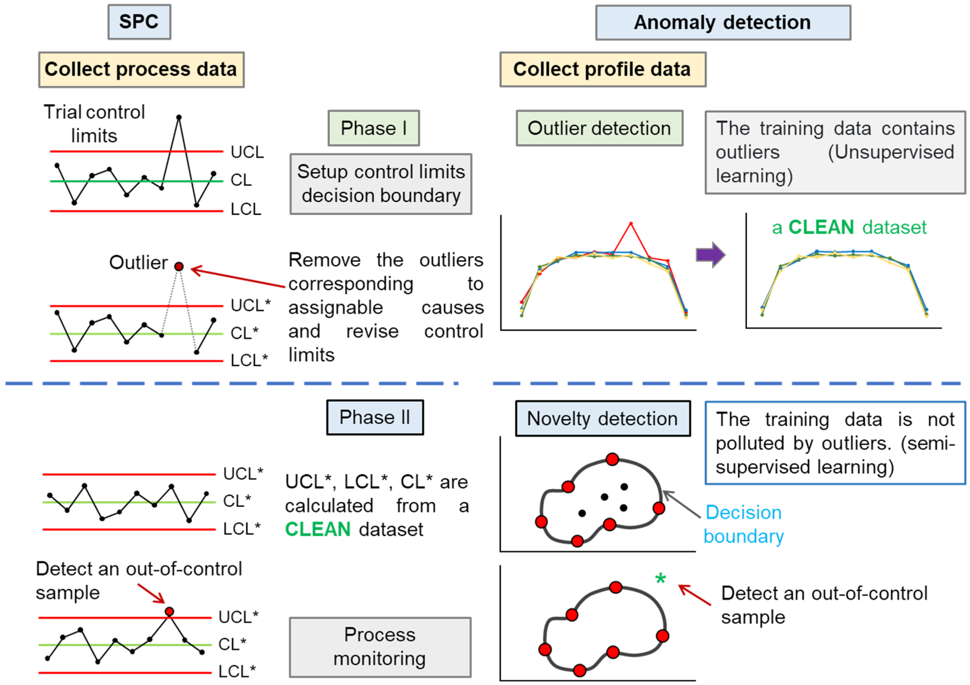
In this study, an anomaly-detection-based method for nonlinear profile monitoring is proposed to deal with the above-mentioned challenges. The concept of anomaly detection is quite similar to that of phase I and phase II applications in SPC. The relationship between the entire profile monitoring procedure and anomaly detection is illustrated in Figure 2. The main aim of phase I is to estimate the control chart parameters using a set of historical data, which usually comprise data from the IC and OOC conditions. In phase II application, we assume control chart parameters are known. In practical applications, the phase II control chart parameters can be determined using the analysis results of phase I. The more accurate the estimation of the control chart parameters in phase I, the better the performance of the phase II control chart.
Anomaly detection involves finding outlier values in a series of data. Novelty detection and outlier-detection algorithms can be applied to identify anomalies [16,17]. In machine learning, the term anomaly detection is often used synonymously with outlier detection [18,19,20,21]. However, some authors distinguish these two terms [16,17]. In this study, we make a distinction between the aforementioned two terms. In outlier detection, the objective is to detect the preexisting outliers in a dataset. In novelty detection, new data are compared with a dataset that does not contain outliers to determine whether the new data are outliers.
In SPC, the dataset collected in phase I may include data from both IC and OOC conditions, and the type of data cannot be known in advance. The aim of phase I is to identify the outliers so as to obtain a clean dataset. As such, phase I analysis corresponds with outlier detection.
The outlier-detection method considered in this study requires defining a parameter called the contamination rate, which refers to the fraction of the total sample size that must be considered outliers. This parameter must be carefully tuned to achieve the best performance. Unfortunately, little research has been conducted to determine the contamination rate. The focus of this study is to propose a method that can accurately estimate the contamination rate to improve the performance of unsupervised algorithms.
The method proposed in this paper consists of three main processes. First, the spline smoothing method is used to smooth a collected set of noisy profiles. Second, a procedure for estimating the proportion of outliers in the dataset is developed. A clustering algorithm is employed to obtain an initial cluster that includes most of the profiles from the IC process. Profiles in the normal cluster are used to determine a baseline profile, and a distance-based decision function is used to identify potential outliers and provide an approximate estimation of the contamination rate. Third, principal component analysis (PCA) is used to identify important features for conducting dimensionality reduction. Researchers in various domains have recognized the importance of high-dimensionality of data [15,22,23]. Several studies have suggested that data should be subjected to dimensionality reduction to decrease the number of coefficients that must be monitored. An outlier-detection algorithm is then employed to identify outlying profiles. Outlier detection can be carried out using several algorithms. In this study, we adopted three commonly used unsupervised algorithms, namely the Local Outlier Factor (LOF), Elliptic Envelope (EE), and Isolation Forest (IF) algorithms.
The rest of this paper is structured as follows. Section 2 describes related work in the field of machine learning in profile monitoring. Section 3 provides a brief overview of anomaly detection and introduces some commonly used outlier-detection algorithms. Section 4 details the proposed method for phase I nonlinear profile monitoring. Section 5 describes the performance of the proposed method and compares it with related methods from the literature. Finally, Section 6 provides the conclusions of this study and recommendations for future research.
2. Related Work
Profile monitoring and anomaly detection of time series data are very similar in concept. The types of outlying profiles studied in previous studies were similar to various types of outliers in time series data. Blázquez-García et al. [24] identified three types of outliers in time series data: point outliers, subsequence outliers, and outlier time series. A point outlier is a data point that acts abnormally at a particular instant in time in comparison with other points in the entire time series (called a global outlier) or its neighbors (called a local outlier). Subsequence outliers are consecutive points in time series whose collective behavior is abnormal even though each point alone is not always a point outlier. “Outlier time series refers” to an entire time series that is an outlier. In profile monitoring, the central segment shifts and local shifts identified in [13] are subsequence outliers, while the vertical shift in [13] is similar to an outlier time series.
Anomaly detection in time series has been extensively studied [16,19,20,21,22,24,25,26,27,28]. Therefore, we only review the application of machine learning algorithms to profile monitoring. Cluster analysis is one of the most commonly adopted machine learning algorithms in phase I profile monitoring. This algorithm is used to divide dataset observations into two groups: IC and OOC data. Ding et al. [15] applied the EM-MIX (expectation-maximization mixture) clustering method [29] to the analysis of profile data.
In [30], authors conducted a study to investigate the effect of phase I estimators on the performance of phase II control charts. They studied the detrimental effect of poor phase I estimators on the performance of phase II control charts in the field of profile monitoring. They found that poor estimators obtained in phase I may produce more false alarms in phase II and take longer to detect OOC profiles.
A typical nonparametric procedure for monitoring profiles in phase I analysis involves constructing a baseline profile that can be compared with all other profiles. A reasonable baseline profile is the average estimated profile of all available profiles. A disadvantage of this approach is that the estimated baseline profile may be biased. This is because it uses all profiles, including any profiles from the OOC process, to obtain the fitted mean. Consequently, the estimated baseline profile shifts toward the profiles collected from the OOC processes, and the estimated baseline profile will be incorrect.
In [31], hierarchical clustering with complete linkage was used to construct a main cluster in order to accurately estimate a baseline curve for later use. They selected the estimated parameter vectors as the input features for the clustering algorithm. Using the concept of a control chart, this method detected OOC profiles by comparing the estimated parameters of each profile to the estimated parameters of a baseline profile. A similar method was introduced by Saremian et al. [32]. They applied a robust cluster-based method in phase I to reduce the impact of data contamination when estimating the generalized linear model parameters.
In [33], the authors developed a nonparametric procedure on the basis of a modified Hausdorff distance and iterative clustering analysis (denoted as MHD-C). They applied the -means clustering algorithm iteratively to detect the OOC profiles present in the collected dataset. Using a simulation study, they show that their method had the benefits of reducing type II errors and more accurately estimating the baseline profile.
Most of the previous studies adopted the -means clustering algorithm because it requires few parameters and is easy to use. For the application of SPC, we only need to divide the data into abnormal and normal categories, and its main parameter can be intuitively set to two. However, the -means algorithm works best in the case of an even cluster size. This algorithm also tends to produce different groups with close numbers of data. That characteristic is not suitable for the phase I application of SPC since in a phase I dataset, most data are usually normal, and only a few are abnormal.
In addition to the -means algorithm, there are many advanced anomaly-detection algorithms in the literature [34,35,36]. However, these are semi-supervised algorithms whose performance is easily affected by outliers in the dataset. These algorithms usually assume that the dataset contains only clean data (either normal class or abnormal class). In addition, one-class SVM is also a commonly used anomaly-detection method, but its performance is easily affected by outliers [37,38], so it is often used when the training dataset is not polluted by outliers.
In the current problem domain, unsupervised algorithms are more suitable than other algorithms since the dataset obtained in phase I may consist of IC and OOC profiles. Furthermore, the type of collected profile is usually not known beforehand. Fernández et al. [39] pointed out that unsupervised algorithms need to determine an important parameter, called the contamination rate, which is equivalent to the proportion of abnormal data in the dataset. They also indicated that the main disadvantage of unsupervised learning is the unsupervised nature and the fact that the hyperparameters must be set appropriately to obtain satisfactory results.
In previous studies, although researchers claimed to use unsupervised learning, they did not have a reasonable proposal for how to determine the contamination rate. Pang et al. [20] even pointed out that there are some studies that refer to methods trained with pure normal training data as unsupervised methods. Roig et al. [40] proposed an ensembled outlier-detection method for wireless sensor networks. They used a set of three well-known unsupervised algorithms; however, they used a clean, labeled dataset to build the model. Cheng et al. [41] proposed a pruning method to determine the proportion of outliers in the dataset. Their method involves calculating an outlier coefficient for each sample in a dataset. An adjustment factor is used to determine the proportion of outliers, with this factor set according to the size and distribution of the dataset.
Dentamaro et al. [42] proposed an ensemble-based anomaly-detection method. They claimed the proposed method can be applied in an unsupervised manner when labels do not exist. However, this method relies on a grid search to find the best hyperparameters that provide the highest accuracy. This means that the method needs to know the proper separation of inliers and outliers before implementation.
Fernández et al. [39] compared many unsupervised outlier-detection methods, but the contamination rate was determined by trying a range of values. This approach is not feasible for phase I profile monitoring for the reasons stated above.
It can be seen from the above literature review that we need an anomaly-detection method that can detect the abnormal data in a dataset in order to establish a clean dataset. Only in this way can we then use more advanced semi-supervised algorithms, such as one-class SVM [43,44] or deep SVDD algorithms [45], to improve the classification accuracy.
3. Theoretical Background
3.1. Anomaly Detection
Anomaly detection refers to the detection of data points or instances that deviate from expected or regular behavior. These irregular instances are often referred to as anomalies, outliers, discordant observations, exceptions, aberrations, surprises, peculiarities, or contaminants in different application domains [25].
There are three types of anomaly-detection methods, depending on the availability of class labels: supervised, semi-supervised and unsupervised methods. Supervised anomaly-detection algorithms assume that fully labeled training and test datasets are available. These algorithms develop a predictive model for abnormal and normal data groups. The primary drawback of supervised anomaly-detection algorithms is that the training dataset contains considerably fewer abnormal instances than normal instances. Semi-supervised anomaly-detection algorithms assume that the dataset includes labeled training data for the normal class only. These algorithms construct a model by using a labeled training dataset that comprises normal data. This model is used to describe normal data and is often called a one-class classifier [26]. Semi-supervised algorithms identify data that deviate from the normal data as anomalies. Unsupervised anomaly-detection algorithms do not need labels in the data, and there is no distinction between the training and test datasets. These algorithms generally assume that the vast majority of instances in a dataset are normal data and search for instances that do not seem to fit with the rest of the dataset. In phase I nonlinear profile monitoring, labeled data are usually unavailable; thus, an unsupervised method must be used in this process.
3.2. Local Outlier Factor
The LOF method is an unsupervised outlier-detection algorithm that evaluates the local density deviation of a given data point in relation to its neighbors [46]. The key concept is to identify samples that have lower density than their neighbors. The output of the LOF algorithm is a local outlier factor score that reflects the abnormality of observations. The LOF algorithm consists of the following steps: (1) determining the -value to select the cluster size; (2) calculating the reachability distance (RD) for each point; (3) calculating the local reachability distance (LRD) value; and (4) calculating the local outlier factor score for each point.
For two given data points and , the distance between them in a Euclidean -dimensional space can be expressed as:
For a given data point , the is defined as the distance between the point and its nearest neighbor. Note that the set of -nearest neighbors includes all points at this distance, which may exceed points when two or more distances are equal. The symbol () represents the set of -nearest neighbors and is also known as -neighbors.
Equation (2) is the reachability distance (RD) of a point with regard to any point . It is defined as the maximum of -distance of and the distance between point and point (i.e., ).
If a point is located within the -neighbors of point , the RD is the -distance of ; otherwise, the RD is set to the actual distance . Figure 3 illustrates the RD of different data points in relation to data point when equals 3 and equals 4. For point in Figure 3, the real distance between and is less than the -distance(); therefore, the RD of point is the -distance(). In the case of , the real distance between and is greater than -distance(), so its RD is the real distance. When the value is large, the objects in the same neighborhood will have similar RD values. This smoothing operation is used to alleviate the variation of for all data points adjacent to point . However, an algorithm with a high value might not recognize local outliers, whereas an algorithm with a small value is sensitive to noise.
The third step of the LOF algorithm is to compute the LRD value. Equation (3) defines the formula for calculating the LRD for each point. It can be seen that the LRD is the inverse of the average reachability distance of a data point from its neighbors. Based on Equation (3), the larger the average RD (i.e., the neighbors are at a greater distance from the point), the smaller the density of points around a particular point. This indicates how far a point is located from the nearest cluster of points. A low LRD means that the nearest cluster is located at a greater distance from the point.
The final step is calculating the LOF score. The formula for calculating the LOF score is defined in Equation (4). It is the ratio of the average LRD of the -neighbors of a data point to the LRD of .
The ratio of the average LRD of neighbors is almost equal to the LRD of a point if the point is a normal instance (since a point has an approximately equal density to its neighbors). In this case, the LOF score is roughly equal to 1. When the point is an outlier, then the LRD of the point will be smaller than the average LRD of neighboring points. In such a case, the LOF score is higher than 1.
One advantage of the LOF algorithm is that it considers both local and global characteristics of the dataset. This means it can achieve a good performance even for datasets in which the outlying samples have different underlying densities.
The LOF algorithm can perform two types of detection, outlier detection and novelty detection. Among them, outlier detection is based on unsupervised learning, while novelty detection is semi-supervised. In this study, the LOF algorithm was implemented using the scikit-learn library [47] and worked as an outlier-detection method.
Some guidelines for determining the range of the neighborhood size are given in [46]. In general, the lower bound on the number of neighbors should be the minimum number of samples in a cluster, and the upper bound should be the maximum number of nearby samples that are likely to be outliers. Unfortunately, such information is usually not available. Even if this information is known, the ideal neighborhood size between the lower and upper bounds remains undetermined. In addition to the neighborhood size, the contamination rate, which defines the ratio of samples in the dataset to be identified as outliers, is another hyperparameter of the LOF algorithm. The above two hyperparameters affect the performance of the LOF algorithm to a great extent; however, limited literature is available regarding the tuning of these parameters in the LOF algorithm for outlier detection. Xu et al. [48] proposed a heuristic methodology to set up the hyperparameters of the LOF algorithm. The key concept is to maximize the difference between predicted outliers and inliers that are nearby the decision boundary.
3.3. Isolation Forest
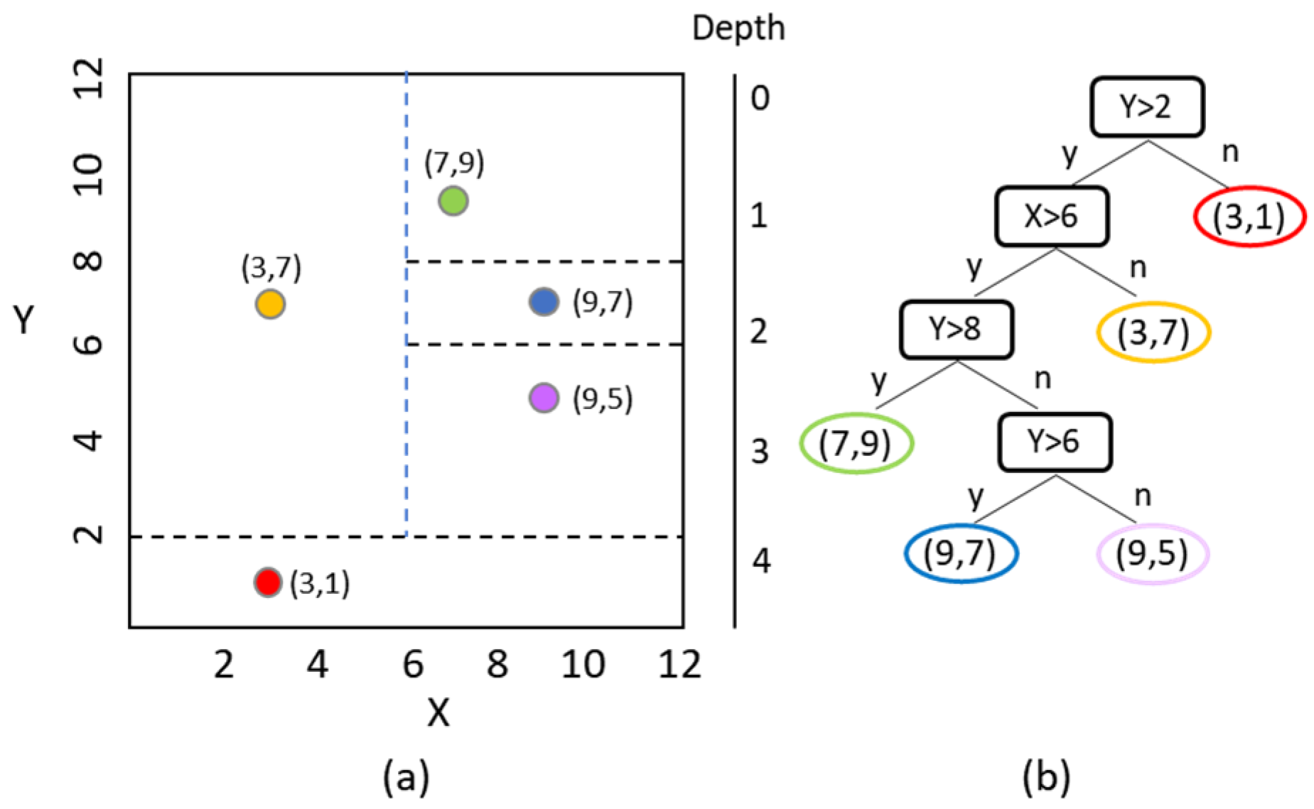
The IF algorithm is considered a tree-based outlier-detection method. It is an unsupervised machine learning algorithm that detects outliers merely on the basis of isolation without using any distance or density measure. This algorithm selects a feature from a given feature set in a random manner, and then randomly picks a split value between the maximum value and minimum value of the selected feature to isolate observations. The partitioning process terminates when the algorithm has isolated all observations or when all remaining observations have the same value. The normality of an observation given a random tree is the number of splits required to isolate the observation, which is equivalent to the path length from the root node to the terminating node containing the observation. The IF algorithm takes the average path length calculated from all the random trees in an isolation forest, constructs a measure of normality, and establishes a decision function. Figure 4 illustrates the concept of an isolation tree.
The contamination rate is a critical hyperparameter when applying the IF model. It is defined as the expected ratio of outliers in the dataset. This parameter varies between 0.0 and 0.5. In this study, the implementation of the IF algorithm was based on the ExtraTreeRegressor ensemble from the scikit-learn library [47].
3.4. Elliptic Envelope
The EE algorithm is an unsupervised machine learning technique that fits a robust covariance estimate to the data. Based on the assumption that the inlier data are normally distributed, it finds the inlier location and covariance in a robust manner without being affected by outliers. The EE algorithm tries to fit an ellipsoid around the data using the minimum covariance determinant [49,50]. The radii of the ellipsoid along each axis are measured in terms of the Mahalanobis distance. The calculated Mahalanobis distances are then used to derive a measure of outlyingness. Instances that fall outside the ellipsoid will be identified as outliers. The algorithm requires a contamination parameter to define the expected proportion of outliers to be detected. In the current study, we applied the EllipticEnvelope function of the scikit-learn covariance module [47] to implement the EE algorithm.
4. Methods
This section describes the proposed approach for the phase I analysis of nonlinear profiles. Moreover, it details a comparison between the performance of the proposed method and other related methods described in the literature.
The proposed method consists of three main processes: smoothing the noisy nonlinear profiles by using the spline smoothing method, estimating the contamination rate, and detecting outliers. Figure 5 displays the framework of the proposed method. Details on each of the aforementioned processes are provided herein.
4.1. Smoothing Profiles
In this study, the dataset consists of profiles, each of which has a length . Thus, the th observed profile is comprised of pairs of points (,), and . The IC relationship between and (i.e., ) is unknown. However, we assume the random error is normally distributed with a mean of zero and a standard deviation of . We also assume the dataset includes both IC and OOC profiles.
The first step of the proposed method is to smooth the profile data using an appropriate spline smoothing method. Our proposed method incorporates a clustering phase to aid in determining the critical parameter known as the contamination rate. The clustering method is used to determine a so-called main cluster that represents profiles of the IC process. Statistical analysis is then conducted to get a rough estimate of the contamination rate on the basis of the distribution of the Euclidean distances calculated from the observed profiles and the baseline profile. The baseline profile is calculated from all the profiles that constitute the main cluster.
In this study, B-spline or basis spline is selected as the smooth function. B-spline is a method of approximating a curve based on given coefficients. The B-spline function can be used to approximate the nonlinear function .The nonlinear function can be represented by
where denote spline coefficients, and are B-spline basis functions of degree and knots .
B-spline basis elements can be expressed as follows:
In the present study, we implemented B-spline using the Python-based SciPy library [51]. The profile data were fitted with a B-spline algorithm, and interpolation profiles were obtained by using the splrep() and BSpline() functions in SciPy. The splrep() function was employed to determine the B-spline representation of the observed profile. The major parameters affecting the interpolation include the degree of the spline, the number of knots and the smoothing condition . The parameter determines the smoothness of the fit. A higher value indicates greater smoothness, whereas a smaller value represents lower smoothness. The BSpline() function was used to evaluate the knot points and coefficients to obtain the fitted values.
4.2. Determining the Contamination Rate
In practical application, the dataset obtained in phase I may consist of IC and OOC profiles. However, the type of collected profiles is usually not known beforehand. Consequently, we need to determine if there are any OOC profiles in the dataset. There are numerous outlier-detection algorithms that have been applied successfully in many application domains, but their performance is highly dependent on the correct setting of hyperparameters. However, the characteristic of the unsupervised outlier-detection models implies that there is a lack of information regarding the true category of each profile for dividing OOC profiles from IC profiles, and as a result, performing optimal hyperparameter estimation is difficult.
In the second process of the proposed method, -means clustering is conducted on the smoothed profiles. In this study, the number of clusters was set to two. Based on the sparsity characteristic of outliers, the ratio of outliers in a dataset is usually relatively low [52,53]. The cluster that contains more than half of the profiles is considered the main cluster, which corresponds to the IC profiles.
In this study, the average of all the profiles in the main cluster was treated as the baseline (reference) profile. We calculated the Euclidean distance between each profile and the baseline profile. A threshold was then determined by considering the average and the standard deviation of the profiles’ distances in the main cluster. We suggest using the percentile of the normal distribution to determine the threshold. If the distances () have a normal distribution, the threshold can be set as , where is the upper percentile of the standard normal distribution, and and are the sample average and standard deviation of the calculated distance , respectively.
After determining the distance threshold, profiles with a distance greater than this threshold were considered OOC profiles. Finally, the contamination rate can be determined by calculating the proportion of the number of profiles exceeding the threshold to the total number of profiles. Note that the above method may overestimate the contamination rate. This is understandable since it includes samples from the set of IC profiles (due to the setting of type I error) as well as the real OOC profiles. A small number of misclassified IC profiles may not cause problems as they can be further verified by human experts. The detected OOC profiles may not yet have assignable causes; therefore, suspected OOC profiles must be analyzed to search for potential assignable causes.
4.3. Detecting Outliers
In the third process of the proposed method, an outlier-detection algorithm is employed to determine the outlying profiles. The contamination rate can be determined by the method described in the aforementioned section. Before applying the outlier-detection algorithm, PCA is conducted to identify important features that reduce the dimensionality of the nonlinear profiles. The key concept behind PCA is to project high-dimensional data on a new coordinate system consisting of principal components (i.e., dimensions), where is usually set to be smaller than the original number of dimensions. In PCA, the principal components are determined by identifying the components that capture the greatest variance in the high-dimensional data.
In this study, we implemented PCA in Python by using the scikit-learn library [47]. The reason for choosing PCA was that it only needs to tune a key parameter, namely the number of components. Furthermore, the number of components to retain can be determined by the total amount of variance explained by the chosen components (typically 85%).
On the basis of a preliminary study, we found that the LOF and EE algorithms can benefit from PCA. However, we noticed that using PCA-processed data in the IF algorithm did not improve its performance. Therefore, we did not apply PCA in the IF algorithm.
5. Results and Discussion
5.1. Data
In the following numerical comparison, we consider a nonlinear profile from the study of Zhang and Albin [54]. This profile has been investigated by several researchers [33,55]. The method proposed in [55] is known as penalized profile outlier detection (PPOD). In order to conduct a direct and fair comparison, we adhered to all the settings and scenarios used in [33,55]. The considered profile has the following functional form:
where , and denotes the random noise of the profile that follows a standard normal distribution with a mean of 0 and standard deviation of 1. There are a total of 100 points in each profile (i.e., ), evenly distributed at intervals of 0.02. Taking the coefficient as the major source of profile variation, the competing methods are evaluated and analyzed when . The profiles with indicate the process is in control.
Figure 6a illustrates the IC and OOC profiles without noise. It is hard to distinguish the IC profile from the OOC profile when random noise exists. The profiles shown in Figure 6b are almost indistinguishable. For this particular profile function, when the value of the coefficient gets larger, the peak and valley points of the entire profile will become closer and less obvious. This phenomenon indicates that it is difficult to differentiate between an IC profile and an OOC profile.
For clarity of presentation, we use the same notation as in [53]. Each dataset consists of non-outlying and outlying profiles where and takes on values 20, 40, or 60. The contamination rate can be defined as . Zou et al. [55] considered a case where , which is probably high for many anomaly-detection problems. Thus, their results are not presented here. Suppose among the IC profiles, profiles are misidentified as OOC profiles, and among the OOC profiles, profiles are correctly identified. When expressed in decimal numbers, the type I and type II errors can be computed as and , respectively.
5.2. Evaluation Metrics
The primary purpose of phase I analysis is to accurately determine and remove OOC profiles to establish a stable IC state model. In related studies, type I and type II errors are usually employed to assess the performance of phase I analysis [33,55]. In this study, we evaluate the proposed method using the standard evaluation technique. Some performance metrics commonly used in machine learning were also adopted. The anomaly-detection performance is usually measured in terms of precision, recall, and score [21,27,28], each of which is defined as follows:
In the field of profile monitoring, outlying profiles are considered as positive class (belonging to the OOC process) and normal profiles (belonging to the IC process) as negative class. True positives (TP) refer to the number of outlier profiles that are successfully detected, false positives (FP) refer to the number of normal profiles that are incorrectly detected as outlying profiles, true negatives (TN) refer to the number of normal profiles that are correctly detected, and false negatives (FN) refer to the number of outlying profiles that are incorrectly detected as normal profiles. The score is the harmonic mean of the precision and recall of a model. A high score indicates that low FP and FN are achieved.
The score is a special case of the general function when . If , recall is considered more important than precision and the priority is to minimize false negatives. In this study, the most commonly used is adopted as the performance metric. The reason for selecting is explained in the following text. It is commonly agreed [33,55] that in phase I monitoring, the type II error (false negative) is more important than the type I error. Typically, the higher the type II error, the more outlying profiles are treated as the IC profiles. Consequently, this will create an inadequate decision function of phase II and deteriorate the performance.
5.3. Results
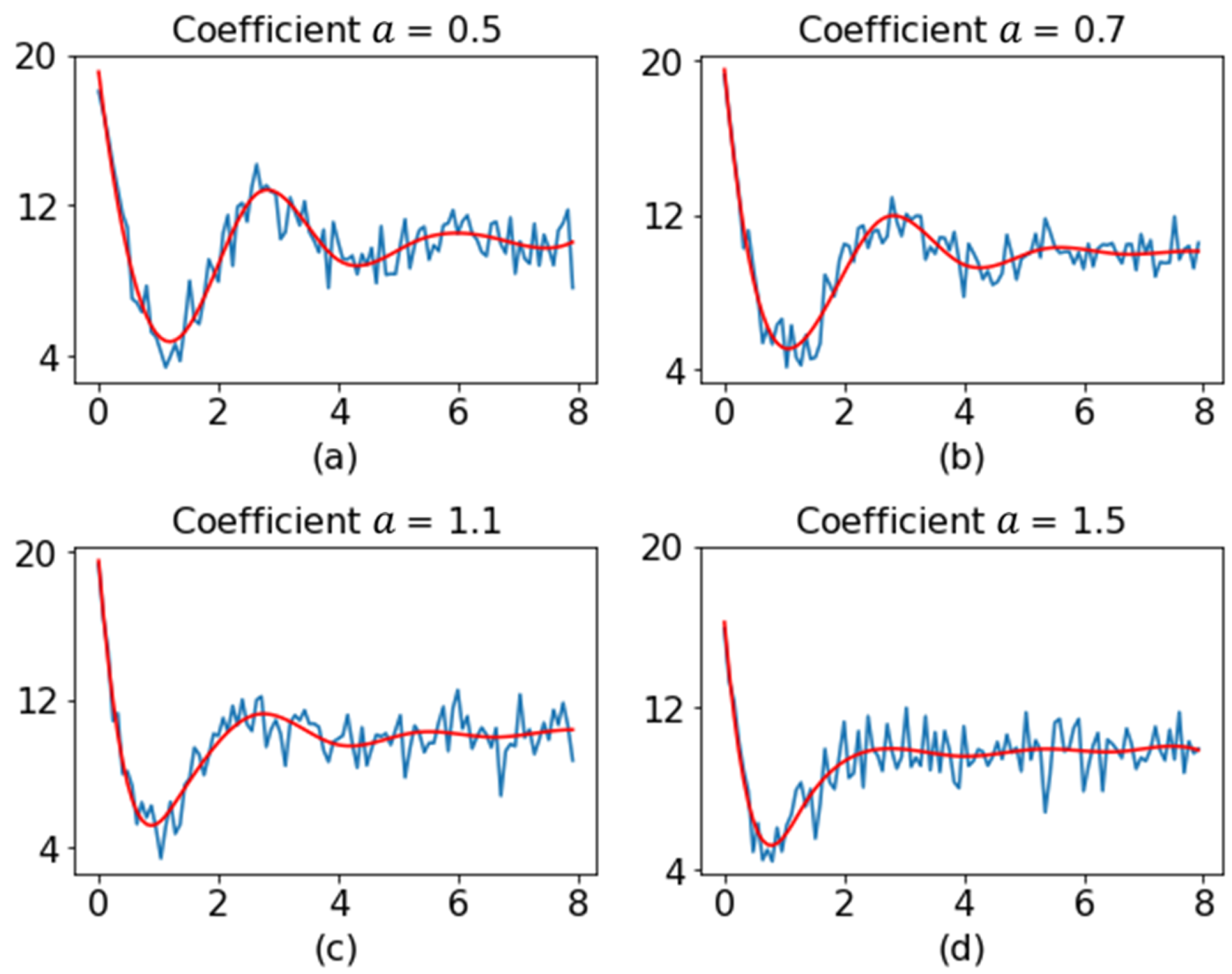
To assess the performance of the proposed method, its performance was compared with those of other methods through simulation. Before moving to the presentation of the results, we describe the choices of parameters of different methods used in this study. The splrep() function from the Scipy library [51] was used to find the B-spline representation of the observed profile data. The key parameters affecting the interpolation include the degree of the spline, the number of knots , and the smoothing condition . In this study, we fixed to 3 (the most commonly used value) and to 5 to get a smoother profile. Moreover, we set (interpolating). Figure 7 shows the original profile and the smoothed profile for different values of coefficient .
In determining the distance threshold, the current study set the type I error in order to be consistent with the study of Zou et al. [55]. Figure 8 depicts histograms of the calculated distances for different contamination rates. In the normality test (Anderson–Darling test), a - greater than the significance level (usually 0.05) indicated the distances had a normal distribution. The results of the normality test conducted in this study indicated that was an appropriate distance threshold.
Most of the parameters of the three outlier-detection algorithms were set to default values, which could provide a satisfactory performance. For the IF algorithm, the number of trees was set to 200. In phase I analysis, the IC data were assumed to indicate the preponderance of the dataset [15]. The -value of the LOF algorithm was chosen to be 120, which was slightly larger than half the number of samples in the dataset.
We now present the results of the comparative study. First, we compare the performance of various methods when the contamination rate is unknown and estimated according to the proposed method described earlier. Table 1, Table 2 and Table 3 present the average type I errors, type II errors, and scores of various considered algorithms, respectively. All results were obtained from the evaluation of 1000 datasets. For a clear comparison, we also provide the standard deviation of each performance metric. In what follows, the results of the MHD-C and PPOD algorithms are presented from [33] and [55], respectively. The results of the LOF, EE, and IF algorithms were obtained in the current research.
When the true contamination rates are 0.1, 0.2, and 0.3, the contamination rates estimated using the proposed approach are 0.15, 0.24, and 0.33, respectively. As shown in Table 1, regardless of the contamination rate, when the coefficient is equal to 0.7, the type I error of LOF is smaller than that of MHD-C. The type I error of MHD-C is rapidly enhanced when the coefficient is large. When the coefficient is greater than 0.7, the type I errors of LOF are larger than those of MHD-C. The type I error of the PPOD algorithm approaches 0.05 only when the coefficient is equal to 0.7. For other values of coefficient , the PPOD algorithm yields a stable type I error but is much greater than 0.05. In all cases, the type I errors of the LOF and EE algorithms are close to the prespecified 0.05. The type I error of the IF algorithm is significantly larger than the prespecified 0.05. As mentioned earlier, using PCA-processed data in the IF algorithm did not improve its performance. Taking the case with parameter , as an example, the type I error of IF is 0.089, while that without PCA is 0.072. Except for the IF algorithm, we notice that the type I errors of other methods start to decrease as becomes larger.
From Table 2, it is readily apparent that regardless of the contamination rate and the size of coefficient , the type II errors of the LOF and EE algorithms are less than or equal to those of MHD-C. LOF and EE perform almost equally well. The PPOD algorithm produces a stable type II error when the coefficient , but performs worse than MHD-C when . In all outlier-detection methods, IF has the highest type II error. Moreover, the type II errors of the different considered algorithms increase with the contamination rate.
Table 3 shows the score of each considered method. For methods MHD-C and PPOD, this study can only use the mean values of the type I and type II errors to estimate the score due to a lack of availability of original data. Therefore, the standard deviation of the value is not provided in Table 3. Several trends can be observed from this table. The scores of the LOF and EE algorithms are unaffected by the size of coefficient and remain stable. The LOF algorithm has higher scores than all the other algorithms; however, when the coefficient increases, the scores of other algorithms increase considerably. This result can be explained by the fact that as the coefficient increases, the type II error decreases substantially, which results in a considerable increase in the score. It is worth noting that when the coefficient , the score of the MHD-C algorithm is considerably lower than that of the LOF and EE algorithms. However, when the coefficient , the scores of the MHD-C algorithm are all close to the ideal value of 1.0.
The variation in the performance of the MHD-C algorithm may be attributed to the method of performance evaluation. The adopted evaluation framework is based on the assumption that there is only one size of coefficient in each dataset. However, in practical applications, each collected dataset may contain a variety of outlying profiles with different sizes of coefficient , and this affects the estimation of type I and type II errors.
Another interesting observation is that the performance of the PPOD and IF algorithms is similar. When the coefficient is equal to 0.7, the scores of both methods are very low, but as the coefficient increases, their scores stabilize.
As the contamination rate increases, the scores of the LOF and EE algorithms increase. This indicates that the LOF and EE algorithms have lower false negative rates. However, the scores of the PPOD and IF algorithms decrease with an increase in the contamination rate. The score of the LOF algorithm is marginally higher than that of the EE algorithm, and these algorithms have similar type I and type II errors. The score of the IF algorithm is substantially lower than those of the other algorithms.
In the above comparisons, type I and type II errors were assessed separately for different parameters . This evaluation method does not quite match the situation of practical application. The dataset collected in SPC phase I usually contains normal profiles and outlying profiles of various variation sizes (different parameter ). The variation of parameter has the greatest impact on type II errors, so we compare the performance of different algorithms when parameter is the smallest (). This represents the most difficult situation to detect. The proposed method achieves a superior performance as compared to traditional methods. The type I error, type II error, and score of LOF are 0.049, 0.001, and 0.951, respectively, and for MHD-C, which is the second best, are 0.081, 0.015, and 0.899, respectively.
We subsequently compared the performance of various methods given known contamination rates. Under this condition, only the three outlier-detection algorithms were are considered. This is because when the contamination rate is known, the outlier-detection algorithms are advantageous compared to the MHD-C and PPOD algorithms, and the comparison results will be biased. Therefore, we chose to compare only outlier-detection algorithms.
Table 4, Table 5 and Table 6 summarizes the type I errors, type II errors, and scores of the three outlier-detection algorithms, respectively. Table 4 indicates that when the contamination rate is less than 0.3 (i.e., ), the type I error of the LOF algorithm is marginally lower than that of the EE algorithm. When the contamination rate is 0.3, the type I error of the EE algorithm is marginally lower than that of the LOF algorithm. Moreover, the type I error of the IF algorithm is considerably higher than those of the other two algorithms.
Table 5 presents the type II errors of the three outlier algorithms. We can see that the results have the same trend as those for the type I errors, that is, the type II error of the LOF algorithm is close to that of the EE algorithm, whereas the IF algorithm has a considerably higher type II error than the other two algorithms. When the coefficient is higher than 0.9, the type II errors of the LOF and EE algorithms approach 0, while the IF algorithm still has a very high type II error. As presented in Table 6, the scores of the LOF and EE algorithms are almost equal to 1 when the coefficient is greater than or equal to 0.9. The IF algorithm has high type I and type II errors and poor performance.
It should be noted that the collected dataset may contain profiles with different sizes of coefficient . The evaluation framework employed in previous relevant studies [33,55] is based on the assumption that only one size of coefficient exists in each dataset. This approach might produce biased estimates of overall performance. The type I error obtained using the method of Nie et al. [33] might be affected by the outlying profiles with the smallest value of coefficient . In contrast, the method proposed in this study can maintain a stable performance under variation of coefficient .
To verify the aforementioned statement, we conducted an additional experiment. For each contamination rate, we generated an additional 1000 datasets, each of which included different values of coefficient . The results of this experiment are shown in Table 7, Table 8 and Table 9. As presented in Table 7, the LOF and EE algorithms keep the same type I error under different values of coefficient . The type I error of the IF algorithm is highly dependent on the value of coefficient . Therefore, the EE and LOF algorithms outperform the IF algorithm. Table 7 and Table 8 indicate that the IF algorithm seems to have the highest type I and type II errors and leads to an unsatisfactory performance, as shown in Table 9. The results in Table 7, Table 8 and Table 9 indicate that the performance of the LOF and EE algorithms is not substantially affected by variations in the magnitudes of the outlier profiles.
When the contamination rate is known, the type I errors of the three outlier-detection algorithms are lower than when the estimated contamination rate is used. This is because the type I error of the proposed method is a fixed value. With known contamination rates, while type I errors are significantly reduced, the type II errors of the three outlier-detection algorithms are also slightly increased.
In all cases, the LOF and EE algorithms have quite close performance, and both substantially outperform the IF algorithm. This result can be attributed to the characteristics of profiles in the OOC state. In the future, different types of profiles and their anomaly types can be studied to compare the performance of various outlier-detection algorithms in further detail.
6. Conclusions
Profile monitoring has attracted considerable research interest recently. Outliers in historical datasets can have detrimental impacts on phase I parameter estimation and phase II monitoring performance. In this study, we presented a phase I analysis procedure for nonlinear profiles by using unsupervised outlier-detection algorithms. The proposed method involves three major processes: profile smoothing, contamination rate estimation, and outlier detection.
The performance of the proposed method was evaluated on a nonlinear profile taken from previous studies. The evaluation results indicate that the proposed method is generally more effective than the existing methods for profile monitoring. These improvements are primarily attributed to the accurate estimation of the contamination rate of the dataset. The LOF algorithm outperformed other competing methods in terms of type I error, type II error, and score. When considering the smallest and hardest-to-detect variation, the type I and type II errors and score of LOF are 0.049, 0.001, and 0.951, respectively, and for MHD-C, which is the second best, are 0.081, 0.015, and 0.899, respectively. We also compared the performance of outlier-detection methods and found that the LOF algorithm outperforms the other two algorithms. The performance of the LOF algorithm is promising when evaluated with known or unknown contamination rates. The results indicate that the proposed method can significantly reduce type II errors, which can help practitioners rapidly remove relevant assignable causes.
We realize that the procedure developed in this study is most appropriate for smooth nonlinear profiles. Many complicated functional forms of nonlinear profiles exist, and further studies should be conducted on these functional forms. Finally, the differences between profiles can be represented by arbitrary functions. Extension from monitoring a global shift to a local shift may be a future research direction.
Future research can also apply the method proposed in this study to build a dataset containing only normal profiles, and then use a semi-supervised algorithm to build the correct decision boundary to detect outlying profiles. When enough normal and outlying profiles are collected or augmented, supervised algorithms can be used to further build improved classification models.
Author Contributions
Conceptualization, C.-S.C.; Methodology, C.-S.C. and P.-W.C.; Software, C.-S.C., P.-W.C. and Y.-T.W.; Formal Analysis, C.-S.C., P.-W.C. and Y.-T.W.; Investigation, C.-S.C. and P.-W.C.; Data Curation, P.-W.C. and Y.-T.W.; Writing—Original Draft Preparation, C.-S.C., P.-W.C. and Y.-T.W.; Writing—Review and Editing, C.-S.C., P.-W.C. and Y.-T.W.; Supervision, C.-S.C. All authors have read and agreed to the published version of the manuscript.
Funding
This research was partially funded by the National Science and Technology Council, Taiwan. (grant number NSTC 111-2221-E-155-028-).
Institutional Review Board Statement
Not applicable.
Informed Consent Statement
Not applicable.
Data Availability Statement
All data generated in this study are available on request from the corresponding author.
Conflicts of Interest
The authors declare no conflict of interest regarding the publication of this manuscript.
References
- Chicken, E.; Pignatiello, J.J., Jr.; Simpson, J.R. Statistical process monitoring of nonlinear profiles using wavelets. J. Qual. Technol. 2009, 41, 198–212. [Google Scholar] [CrossRef]
- Jensen, W.A.; Grimshaw, S.D.; Espen, B. Nonlinear profile monitoring for oven-temperature data. J. Qual. Technol. 2016, 48, 84–97. [Google Scholar] [CrossRef]
- Woodall, W.H.; Spitzner, D.J.; Montgomery, D.C.; Gupta, S. Using control charts to monitor process and product quality profiles. J. Qual. Technol. 2004, 36, 309–320. [Google Scholar] [CrossRef]
- Maleki, M.R.; Amiri, A.; Castagliola, P. An overview on recent profile monitoring papers (2008–2018) based on conceptual classification scheme. Comput. Ind. Eng. 2018, 126, 705–728. [Google Scholar] [CrossRef]
- Stover, F.S.; Brill, R.V. Statistical quality control applied to ion chromatography calibrations. J. Chromatogr. A 1998, 804, 37–43. [Google Scholar] [CrossRef]
- Kang, L.; Albin, S.L. On-line monitoring when the process yields a linear profile. J. Qual. Technol. 2000, 32, 418–426. [Google Scholar] [CrossRef]
- Kim, K.; Mahmoud, M.A.; Woodall, W.H. On the monitoring of linear profiles. J. Qual. Technol. 2003, 35, 317–328. [Google Scholar] [CrossRef]
- Mahmoud, M.A.; Parker, P.A.; Woodall, W.H.; Hawkins, D.M. A change point method for linear profile data. Qual. Reliab. Eng. Int. 2007, 23, 247–268. [Google Scholar] [CrossRef]
- Williams, J.D.; Woodall, W.H.; Birch, J.B. Statistical monitoring of nonlinear product and process quality profiles. Qual. Reliab. Eng. Int. 2007, 23, 925–941. [Google Scholar] [CrossRef]
- Gardner, M.M.; Lu, J.C.; Gyurcsik, R.S.; Wortman, J.J.; Hornung, B.E.; Heinisch, H.H.; Rying, E.A.; Rao, S.; Davis, J.C.; Mozumder, P.K. Equipment fault detection using spatial signatures. IEEE Trans. Compon. Packag. Manuf. Technol. Part C 1997, 20, 295–304. [Google Scholar] [CrossRef]
- Fan, J. Test of significance based on wavelet thresholding and Neyman’s truncation. J. Am. Stat. Assoc. 1996, 91, 674–688. [Google Scholar] [CrossRef]
- Jin, J.; Shi, J. Automatic feature extraction of waveform signals for in-process diagnostic performance improvement. J. Intell. Manuf. 2001, 12, 257–268. [Google Scholar] [CrossRef]
- Jeong, M.K.; Lu, J.C.; Wang, N. Wavelet-based SPC procedure for complicated functional data. Int. J. Prod. Res. 2006, 44, 729–744. [Google Scholar] [CrossRef]
- Woodall, W.H. Controversies and contradictions in statistical process control. J. Qual. Technol. 2000, 32, 341–350. [Google Scholar] [CrossRef]
- Ding, Y.; Zeng, L.; Zhou, S. Phase I analysis for monitoring nonlinear profiles in manufacturing processes. J. Qual. Technol. 2006, 38, 199–216. [Google Scholar] [CrossRef]
- Hodge, V.; Austin, J. A survey of outlier detection methodologies. Artif. Intell. Rev. 2004, 22, 85–126. [Google Scholar] [CrossRef]
- Pattisahusiwa, A.; Purqon, A. Comparison of outliers and novelty detection to identify ionospheric TEC irregularities during geomagnetic storm and substorm. J. Phys. Conf. Ser. 2016, 739, 012015. [Google Scholar] [CrossRef]
- Miljković, D. Review of novelty detection methods. In Proceedings of the 33rd International Convention MIPRO, Opatija, Croatia, 29 July 2010; pp. 593–598. [Google Scholar]
- Chalapathy, R.; Chawla, S. Deep learning for anomaly detection: A survey. arXiv 2019, arXiv:1901.03407. [Google Scholar]
- Pang, G.; Shen, C.; Cao, L.; Hengel, A.V.D. Deep learning for anomaly detection: A review. ACM Comput. Surv. 2021, 54, 1–38. [Google Scholar] [CrossRef]
- Ruff, L.; Kauffmann, J.R.; Vandermeulen, R.A.; Montavon, G.; Samek, W.; Kloft, M.; Müller, K.R. A unifying review of deep and shallow anomaly detection. Proc. IEEE 2021, 109, 756–795. [Google Scholar] [CrossRef]
- Thudumu, S.; Branch, P.; Jin, J.; Singh, J.J. A comprehensive survey of anomaly detection techniques for high dimensional big data. J. Big Data 2020, 7, 42. [Google Scholar] [CrossRef]
- Ebadi, M.; Chenouri, S.; Steiner, S.H. Phase I analysis of high-dimensional multivariate processes in the presence of outliers. arXiv 2021, arXiv:2110.13689. [Google Scholar]
- Blázquez-García, A.; Conde, A.; Mori, U.; Lozano, J.A. A review on outlier/anomaly detection in time series data. ACM Comput. Surv. 2021, 54, 1–33. [Google Scholar] [CrossRef]
- Chandola, V.; Banerjee, A.; Kumar, V. Anomaly detection: A survey. ACM Comput. Surv. 2009, 41, 1–58. [Google Scholar] [CrossRef]
- Pimentel, M.A.; Clifton, D.A.; Clifton, L.; Tarassenko, L. A review of novelty detection. Signal Process. 2014, 99, 215–249. [Google Scholar] [CrossRef]
- Al-amri, R.; Murugesan, R.K.; Man, M.; Abdulateef, A.F.; Al-Sharafi, M.A.; Alkahtani, A.A. A review of machine learning and deep learning techniques for anomaly detection in IoT data. Appl. Sci. 2021, 11, 5320. [Google Scholar] [CrossRef]
- Choi, K.; Yi, J.; Park, C.; Yoon, S. Deep learning for anomaly detection in time-series data: Review, analysis, and guidelines. IEEE Access 2021, 9, 120043–120065. [Google Scholar] [CrossRef]
- McLachlan, G.; Peel, D. Finite Mixture Models; John Wiley & Sons, Ltd.: New York, NY, USA, 2000. [Google Scholar]
- Chen, Y.; Birch, B.; Woodall, W.H. Effect of Phase I estimation on Phase II control chart performance with profile data. Qual. Reliab. Eng. Int. 2016, 32, 79–87. [Google Scholar] [CrossRef]
- Chen, Y.; Birch, J.B.; Woodall, W.H. Cluster-based profile analysis in phase I. J. Qual. Technol. 2015, 47, 14–29. [Google Scholar] [CrossRef]
- Saremian, D.; Noorossana, R.; Raissi, S.; Soleimani, P. Robust cluster-based method for monitoring generalized linear profiles in phase I. J. Ind. Eng. Int. 2021, 17, 88–97. [Google Scholar]
- Nie, B.; Liu, D.; Liu, X.; Ye, W. Phase I non-linear profiles monitoring using a modified Hausdorff distance algorithm and clustering analysis. Int. J. Qual. Reliab. Manag. 2021, 38, 536–550. [Google Scholar] [CrossRef]
- Mao, W.; Shi, H.; Wang, G.; Liang, X. Unsupervised deep multitask anomaly detection with robust alarm strategy for online evaluation of bearing early fault occurrence. IEEE Trans. Instrum. Meas. 2022, 71, 3520713. [Google Scholar] [CrossRef]
- Velasco-Gallego, C.; Lazakis, I. RADIS: A real-time anomaly detection intelligent system for fault diagnosis of marine machinery. Expert Syst. Appl. 2022, 204, 117634. [Google Scholar] [CrossRef]
- Du, W.; Guo, Z.; Li, C.; Gong, X.; Pu, Z. From anomaly detection to novel fault discrimination for wind turbine gearboxes with a sparse isolation encoding forest. IEEE Trans. Instrum. Meas. 2022, 71, 2512710. [Google Scholar] [CrossRef]
- Tian, Y.; Mirzabagheri, M.; Bamakan, S.M.H.; Wang, H.; Qu, Q. Ramp loss one-class support vector machine; a robust and effective approach to anomaly detection problems. Neurocomputing 2018, 310, 223–235. [Google Scholar] [CrossRef]
- Shieh, A.D.; Kamm, D.F. Ensembles of one class support vector machines. In Multiple Classifier Systems; Benediktsson, J.A., Kittler, J., Roli, F., Eds.; Springer: Berlin/Heidelberg, Germany, 2009; Volume 5519, pp. 181–190. [Google Scholar]
- Fernández, A.; Bella, J.; Dorronsoro, J.R. Supervised outlier detection for classification and regression. Neurocomputing 2022, 486, 77–92. [Google Scholar] [CrossRef]
- Roig, M.; Catalan, M.; Gastón, B. Ensembled outlier detection using multi-variable correlation in WSN through unsupervised learning techniques. In Proceedings of the 4th International Conference on Internet of Things, Big Data and Security (IoTBDS), Heraklion, Crete, Greece, 2–4 May 2019; pp. 38–48. [Google Scholar]
- Cheng, Z.; Zou, C.; Dong, J. Outlier detection using isolation forest and local outlier factor. In Proceedings of the International Conference on Research in Adaptive and Convergent Systems, Chongqing, China, 24–27 September 2019; pp. 161–168. [Google Scholar]
- Dentamaro, V.; Convertini, V.N.; Galantucci, S.; Giglio, P.; Palmisano, T.; Pirlo, G. Ensemble consensus: An unsupervised algorithm for anomaly detection in network security data. In Proceedings of the Italian Conference on Cybersecurity (ITASEC), Virtual, 7–9 April 2021; pp. 309–318. [Google Scholar]
- Schölkopf, B.; Platt, J.C.; Shawe-Taylor, J.C.; Smola, A.J.; Williamson, R.C. Estimating the Support of a High-Dimensional Distribution. Neural Comput. 2001, 13, 1443–1471. [Google Scholar] [CrossRef]
- Tax, D.M.J.; Duin, R.P.W. Support vector data description. Mach. Learn. 2004, 54, 45–66. [Google Scholar] [CrossRef]
- Ruff, L.; Vandermeulen, R.A.; Görnitz, N.; Deecke, L.; Siddiqui, S.A.; Binder, A.; Müller, E.; Kloft, M. Deep One-Class Classification. In Proceedings of the 35th International Conference on Machine Learning, Stockholm, Sweden, 10–15 July 2018; pp. 4393–4402. [Google Scholar]
- Breunig, M.M.; Kriegel, H.P.; Ng, R.T.; Sander, J. LOF: Identifying density-based local outliers. In Proceedings of the 2000 ACM SIGMOD International Conference on Management of Data, Dallas, TX, USA, 15–18 May 2000; pp. 93–104. [Google Scholar]
- Pedregosa, F.; Varoquaux, G.; Gramfort, A.; Michel, V.; Thirion, B.; Grisel, O.; Blondel, M.; Prettenhofer, P.; Weiss, R.; Dubourg, V.; et al. Scikit-learn: Machine Learning in Python. J. Mach. Learn. Res. 2011, 12, 2825–2830. [Google Scholar]
- Xu, Z.; Kakde, D.; Chaudhuri, A. Automatic hyperparameter tuning method for local outlier factor. In Proceedings of the 2019 IEEE International Conference on Big Data, Los Angeles, CA, USA, 9–12 December 2019; pp. 4201–4207. [Google Scholar]
- Rousseeuw, P.J. Least median of squares regression. J. Am. Stat. Assoc. 1984, 79, 871–880. [Google Scholar] [CrossRef]
- Rousseeuw, P.J.; Driessen, K.V. A fast algorithm for the minimum covariance determinant estimator. Technometrics 1999, 41, 212–223. [Google Scholar] [CrossRef]
- Virtanen, P.; Gommers, R.; Oliphant, T.E.; Haberland, M.; Reddy, T.; Cournapeau, D.; Burovski, E.; Peterson, P.; Weckesser, W.; Bright, J.; et al. SciPy 1.0: Fundamental algorithms for scientific computing in Python. Nat. Methods 2020, 17, 261–272. [Google Scholar] [CrossRef] [PubMed]
- Wang, K.; Jiang, W. High-dimensional process monitoring and fault isolation via variable selection. J. Qual. Technol. 2009, 41, 247–258. [Google Scholar] [CrossRef]
- Zou, C.; Qiu, P. Multivariate statistical process control using LASSO. J. Am. Stat. Assoc. 2009, 104, 1586–1596. [Google Scholar] [CrossRef]
- Zhang, H.; Albin, S. Detecting outliers in complex profiles using a χ2 control chart method. IIE Trans. 2009, 41, 335–345. [Google Scholar] [CrossRef]
- Zou, C.; Tseng, S.T.; Wang, Z. Outlier detection in general profiles using penalized regression method. IIE Trans. 2014, 46, 106–117. [Google Scholar] [CrossRef]
- Taha, A.A.; Hanbury, A. Metrics for evaluating 3D medical image segmentation: Analysis, selection, and tool. BMC Med. Imaging 2015, 15, 29. [Google Scholar] [CrossRef]
- Tharwat, A. Classification assessment methods. Appl. Comput. Inform. 2020, 17, 168–192. [Google Scholar] [CrossRef]
Figure 1.
Oven temperature profile studied by Jensen et al. [2]. The blue line represents the in-control (IC) profile and the red line represents the out-of-control (OOC) profile.
Figure 1.
Oven temperature profile studied by Jensen et al. [2]. The blue line represents the in-control (IC) profile and the red line represents the out-of-control (OOC) profile.

Figure 2.
Comparison between statistical process control (SPC) and anomaly detection. UCL, CL, and LCL represent the upper control limit, center line, and lower control limit, respectively. UCL*, CL*, and LCL* denote the modified upper control limit, center line, and lower control limit, respectively.

Figure 3.
Reachability distance (RD) when . Points – have the same RD, and is not a -nearest neighbor.
Figure 3.
Reachability distance (RD) when . Points – have the same RD, and is not a -nearest neighbor.

Figure 4.
Concept of an isolation tree: (a) data points and isolation operations; (b) binary tree and the isolated point.
Figure 4.
Concept of an isolation tree: (a) data points and isolation operations; (b) binary tree and the isolated point.

Figure 5.
Framework of the proposed method.

Figure 6.
Nonlinear profiles examined in this study. (a) Nonlinear profiles without noise; (b) Nonlinear profiles with noise added.
Figure 6.
Nonlinear profiles examined in this study. (a) Nonlinear profiles without noise; (b) Nonlinear profiles with noise added.

Figure 7.
Original profiles and smoothed profiles. (a–d) are examples of profiles with coefficients of 0.5, 0.7, 1.1 and 1.5, respectively. In subplots (a–d), the blue lines denote the original profiles and red lines represent the smoothed profiles.
Figure 7.
Original profiles and smoothed profiles. (a–d) are examples of profiles with coefficients of 0.5, 0.7, 1.1 and 1.5, respectively. In subplots (a–d), the blue lines denote the original profiles and red lines represent the smoothed profiles.

Figure 8.
Results of normality test (coefficient ).


Table 1.
Type I error of each considered method under different estimated contamination rates and different magnitudes of coefficient .
Table 1.
Type I error of each considered method under different estimated contamination rates and different magnitudes of coefficient .
| Coefficient | |||||||||||
|---|---|---|---|---|---|---|---|---|---|---|---|
| Method | 0.7 | 0.9 | 1.1 | 1.3 | 1.5 | ||||||
| MHD-C | 20 | 0.142 | (0.083) | 0.005 | (0.006) | 0 | (0.003) | 0 | (0.002) | 0 | (0.001) |
| PPOD | 0.061 | (0.020) | 0.067 | (0.022) | 0.066 | (0.023) | 0.067 | (0.022) | 0.067 | (0.022) | |
| LOF | 0.054 | (0.002) | 0.054 | (0.003) | 0.054 | (0.002) | 0.054 | (0.003) | 0.053 | (0.004) | |
| EE | 0.056 | (0) | 0.056 | (0) | 0.056 | (0) | 0.056 | (0) | 0.056 | (0) | |
| IF | 0.072 | (0.007) | 0.056 | (0) | 0.056 | (0) | 0.056 | (0) | 0.056 | (0) | |
| MHD-C | 40 | 0.057 | (0.029) | 0.005 | (0.006) | 0 | (0.002) | 0 | (0.001) | 0 | (0.001) |
| PPOD | 0.050 | (0.021) | 0.067 | (0.022) | 0.066 | (0.023) | 0.066 | (0.023) | 0.066 | (0.023) | |
| LOF | 0.049 | (0.002) | 0.049 | (0.002) | 0.048 | (0.003) | 0.048 | (0.003) | 0.048 | (0.003) | |
| EE | 0.050 | (0) | 0.050 | (0) | 0.050 | (0) | 0.050 | (0) | 0.050 | (0) | |
| IF | 0.128 | (0.008) | 0.081 | (0.007) | 0.074 | (0.007) | 0.066 | (0.008) | 0.069 | (0.006) | |
| MHD-C | 60 | 0.045 | (0.028) | 0.004 | (0.006) | 0.001 | (0.003) | 0 | (0.002) | 0.001 | (0.002) |
| PPOD | 0.041 | (0.018) | 0.065 | (0.025) | 0.065 | (0.025) | 0.064 | (0.024) | 0.065 | (0.024) | |
| LOF | 0.043 | (0.003) | 0.042 | (0.003) | 0.042 | (0.002) | 0.041 | (0.003) | 0.041 | (0.003) | |
| EE | 0.044 | (0.002) | 0.043 | (0) | 0.043 | (0) | 0.043 | (0) | 0.043 | (0) | |
| IF | 0.214 | (0.018) | 0.171 | (0.017) | 0.153 | (0.014) | 0.154 | (0.023) | 0.144 | (0.019) | |
Numbers in parentheses denote standard deviations.
Table 2.
Type II error of each considered method under different estimated contamination rates and different magnitudes of coefficient .
Table 2.
Type II error of each considered method under different estimated contamination rates and different magnitudes of coefficient .
| Coefficient | |||||||||||
|---|---|---|---|---|---|---|---|---|---|---|---|
| Method | 0.7 | 0.9 | 1.1 | 1.3 | 1.5 | ||||||
| MHD-C | 20 | 0.006 | (0.016) | 0.002 | (0.009) | 0 | (0) | 0 | (0) | 0 | (0) |
| PPOD | 0.366 | (0.141) | 0.001 | (0.007) | 0 | (0) | 0 | (0) | 0 | (0) | |
| LOF | 0 | (0) | 0 | (0) | 0 | (0) | 0 | (0) | 0 | (0) | |
| EE | 0 | (0) | 0 | (0) | 0 | (0) | 0 | (0) | 0 | (0) | |
| IF | 0.150 | (0.067) | 0 | (0) | 0 | (0) | 0 | (0) | 0 | (0) | |
| MHD-C | 40 | 0.016 | (0.021) | 0.002 | (0.008) | 0 | (0) | 0 | (0) | 0 | (0) |
| PPOD | 0.510 | (0.134) | 0.001 | (0.005) | 0 | (0) | 0 | (0) | 0 | (0) | |
| LOF | 0 | (0) | 0 | (0) | 0 | (0) | 0 | (0) | 0 | (0) | |
| EE | 0 | (0) | 0 | (0) | 0 | (0) | 0 | (0) | 0 | (0) | |
| IF | 0.310 | (0.032) | 0.125 | (0.026) | 0.098 | (0.030) | 0.065 | (0.034) | 0.075 | (0.024) | |
| MHD-C | 60 | 0.022 | (0.02) | 0.001 | (0.005) | 0 | (0.002) | 0 | (0.002) | 0 | (0) |
| PPOD | 0.724 | (0.105) | 0.001 | (0.004) | 0 | (0) | 0 | (0) | 0 | (0) | |
| LOF | 0.002 | (0.005) | 0 | (0) | 0 | (0) | 0 | (0) | 0 | (0) | |
| EE | 0.002 | (0.005) | 0 | (0) | 0 | (0) | 0 | (0) | 0 | (0) | |
| IF | 0.398 | (0.042) | 0.298 | (0.040) | 0.257 | (0.032) | 0.260 | (0.053) | 0.235 | (0.045) | |
Numbers in parentheses denote standard deviations.
Table 3.
score of each considered method under different estimated contamination rates and different magnitudes of coefficient .
Table 3.
score of each considered method under different estimated contamination rates and different magnitudes of coefficient .
| Coefficient | |||||||||||
|---|---|---|---|---|---|---|---|---|---|---|---|
| Method | 0.7 | 0.9 | 1.1 | 1.3 | 1.5 | ||||||
| MHD-C | 20 | 0.792 | 0.990 | 1.000 | 1.000 | 1.000 | |||||
| PPOD | 0.612 | 0.892 | 0.899 | 0.892 | 0.892 | ||||||
| LOF | 0.911 | (0.003) | 0.911 | (0.003) | 0.912 | (0.003) | 0.912 | (0.003) | 0.912 | (0.003) | |
| EE | 0.909 | (0) | 0.909 | (0) | 0.909 | (0) | 0.909 | (0) | 0.909 | (0) | |
| IF | 0.773 | (0.061) | 0.909 | (0) | 0.909 | (0) | 0.909 | (0) | 0.909 | (0) | |
| MHD-C | 40 | 0.944 | 0.994 | 1.000 | 1.000 | 1.000 | |||||
| PPOD | 0.522 | 0.948 | 0.950 | 0.950 | 0.950 | ||||||
| LOF | 0.962 | (0.001) | 0.962 | (0.001) | 0.963 | (0.002) | 0.963 | (0.002) | 0.963 | (0.002) | |
| EE | 0.962 | (0) | 0.962 | (0) | 0.962 | (0) | 0.962 | (0) | 0.962 | (0) | |
| IF | 0.664 | (0.041) | 0.841 | (0.041) | 0.869 | (0.037) | 0.893 | (0.030) | 0.898 | (0.024) | |
| MHD-C | 60 | 0.962 | 0.997 | 0.999 | 1.000 | 0.999 | |||||
| PPOD | 0.316 | 0.970 | 0.971 | 0.971 | 0.971 | ||||||
| LOF | 0.979 | (0.005) | 0.981 | (0.001) | 0.981 | (0.001) | 0.981 | (0.001) | 0.981 | (0.001) | |
| EE | 0.979 | (0.004) | 0.980 | (0) | 0.980 | (0) | 0.980 | (0) | 0.980 | (0) | |
| IF | 0.590 | (0.039) | 0.688 | (0.035) | 0.729 | (0.035) | 0.726 | (0.035) | 0.750 | (0.035) | |
Numbers in parentheses denote standard deviations.
Table 4.
Type I error of the three outlier-detection algorithms under the assumption that the contamination rate is known.
Table 4.
Type I error of the three outlier-detection algorithms under the assumption that the contamination rate is known.
| Coefficient | |||||||||||
|---|---|---|---|---|---|---|---|---|---|---|---|
| Method | 0.7 | 0.9 | 1.1 | 1.3 | 1.5 | ||||||
| LOF | 20 | 0.001 | (0.002) | 0 | (0) | 0 | (0) | 0 | (0) | 0 | (0) |
| EE | 0.001 | (0.002) | 0 | (0) | 0 | (0) | 0 | (0) | 0 | (0) | |
| IF | 0.029 | (0.008) | 0.011 | (0.006) | 0.006 | (0.004) | 0.003 | (0.004) | 0.002 | (0.003) | |
| LOF | 40 | 0.002 | (0.004) | 0 | (0) | 0 | (0) | 0 | (0) | 0 | (0) |
| EE | 0.003 | (0.004) | 0 | (0) | 0 | (0) | 0 | (0) | 0 | (0) | |
| IF | 0.093 | (0.013) | 0.059 | (0.010) | 0.041 | (0.011) | 0.038 | (0.008) | 0.037 | (0.010) | |
| LOF | 60 | 0.006 | (0.007) | 0 | (0) | 0 | (0) | 0 | (0) | 0 | (0) |
| EE | 0.005 | (0.007) | 0 | (0) | 0 | (0) | 0 | (0) | 0 | (0) | |
| IF | 0.189 | (0.012) | 0.148 | (0.016) | 0.129 | (0.012) | 0.130 | (0.013) | 0.124 | (0.012) | |
Numbers in parentheses denote standard deviations.
Table 5.
Type II error of the three outlier-detection algorithms under the assumption that the contamination rate is known.
Table 5.
Type II error of the three outlier-detection algorithms under the assumption that the contamination rate is known.
| Coefficient | |||||||||||
|---|---|---|---|---|---|---|---|---|---|---|---|
| Method | 0.7 | 0.9 | 1.1 | 1.3 | 1.5 | ||||||
| LOF | 20 | 0.005 | (0.016) | 0 | (0) | 0 | (0) | 0 | (0) | 0 | (0) |
| EE | 0.008 | (0.018) | 0 | (0) | 0 | (0) | 0 | (0) | 0 | (0) | |
| IF | 0.260 | (0.070) | 0.100 | (0.058) | 0.055 | (0.037) | 0.025 | (0.035) | 0.015 | (0.024) | |
| LOF | 40 | 0.010 | (0.017) | 0 | (0) | 0 | (0) | 0 | (0) | 0 | (0) |
| EE | 0.011 | (0.015) | 0 | (0) | 0 | (0) | 0 | (0) | 0 | (0) | |
| IF | 0.370 | (0.051) | 0.235 | (0.039) | 0.165 | (0.043) | 0.150 | (0.033) | 0.149 | (0.040) | |
| LOF | 60 | 0.017 | (0.018) | 0 | (0) | 0 | (0) | 0 | (0) | 0 | (0) |
| EE | 0.012 | (0.016) | 0 | (0) | 0 | (0) | 0 | (0) | 0 | (0) | |
| IF | 0.440 | (0.029) | 0.345 | (0.038) | 0.300 | (0.039) | 0.303 | (0.031) | 0.288 | (0.027) | |
Numbers in parentheses denote standard deviations.
Table 6.
score of the three outlier-detection algorithms under the assumption that the contamination rate is known.
Table 6.
score of the three outlier-detection algorithms under the assumption that the contamination rate is known.
| Coefficient | |||||||||||
|---|---|---|---|---|---|---|---|---|---|---|---|
| Method | 0.7 | 0.9 | 1.1 | 1.3 | 1.5 | ||||||
| LOF | 20 | 0.995 | (0.016) | 1.000 | (0) | 1.000 | (0) | 1.000 | (0) | 1.000 | (0) |
| EE | 0.993 | (0) | 1.000 | (0) | 1.000 | (0) | 1.000 | (0) | 1.000 | (0) | |
| IF | 0.580 | (0.180) | 0.853 | (0.082) | 0.935 | (0.043) | 0.970 | (0.034) | 0.983 | (0.025) | |
| LOF | 40 | 0.991 | (0.017) | 1.000 | (0) | 1.000 | (0) | 1.000 | (0) | 1.000 | (0) |
| EE | 0.989 | (0.015) | 1.000 | (0) | 1.000 | (0) | 1.000 | (0) | 1.000 | (0) | |
| IF | 0.539 | (0.103) | 0.753 | (0.048) | 0.835 | (0.043) | 0.850 | (0.033) | 0.851 | (0.033) | |
| LOF | 60 | 0.984 | (0.017) | 1.000 | (0) | 1.000 | (0) | 1.000 | (0) | 1.000 | (0) |
| EE | 0.988 | (0.016) | 1.000 | (0) | 1.000 | (0) | 1.000 | (0) | 1.000 | (0) | |
| IF | 0.504 | (0.070) | 0.641 | (0.046) | 0.690 | (0.046) | 0.699 | (0.032) | 0.703 | (0.032) | |
Numbers in parentheses denote standard deviations.
Table 7.
Type I error of the three outlier-detection algorithms when the dataset is contaminated by profiles with different magnitudes of coefficient .
Table 7.
Type I error of the three outlier-detection algorithms when the dataset is contaminated by profiles with different magnitudes of coefficient .
| Contamination Rate | IF | EE | LOF | |||
|---|---|---|---|---|---|---|
| 0.1 (actual) | 0.013 | (0.005) | 0.001 | (0.002) | 0.001 | (0.002) |
| 0.15 (estimated) | 0.059 | (0.003) | 0.056 | (0) | 0.053 | (0.003) |
| 0.2 (actual) | 0.040 | (0.014) | 0.000 | (0.001) | 0.000 | (0.001) |
| 0.24 (estimated) | 0.073 | (0.011) | 0.050 | (0) | 0.049 | (0.003) |
| 0.3 (actual) | 0.095 | (0.015) | 0.001 | (0.003) | 0.000 | (0.002) |
| 0.33 (estimated) | 0.118 | (0.019) | 0.043 | (0) | 0.041 | (0.003) |
Numbers in parentheses denote standard deviations.
Table 8.
Type II error of the three outlier-detection algorithms when the dataset is contaminated by profiles with different magnitudes of coefficient .
Table 8.
Type II error of the three outlier-detection algorithms when the dataset is contaminated by profiles with different magnitudes of coefficient .
| Contamination Rate | IF | EE | LOF | |||
|---|---|---|---|---|---|---|
| 0.1 (actual) | 0.120 | (0.041) | 0.005 | (0.015) | 0.005 | (0.015) |
| 0.15 (estimated) | 0.035 | (0.029) | 0 | (0) | 0 | (0) |
| 0.2 (actual) | 0.160 | (0.054) | 0.001 | (0.006) | 0.001 | (0.006) |
| 0.24 (estimated) | 0.094 | (0.042) | 0 | (0) | 0 | (0) |
| 0.3 (actual) | 0.223 | (0.034) | 0.001 | (0.004) | 0.001 | (0.004) |
| 0.33 (estimated) | 0.174 | (0.044) | 0 | (0) | 0 | (0) |
Numbers in parentheses denote standard deviations.
Table 9.
score of the three outlier-detection algorithms when the dataset is contaminated by profiles with different magnitudes of coefficient .
Table 9.
score of the three outlier-detection algorithms when the dataset is contaminated by profiles with different magnitudes of coefficient .
| Contamination Rate | IF | EE | LOF | |||
|---|---|---|---|---|---|---|
| 0.1 (actual) | 0.880 | (0.041) | 0.995 | (0.015) | 0.995 | (0.015) |
| 0.15 (estimated) | 0.877 | (0.026) | 0.909 | (0) | 0.913 | (0.005) |
| 0.2 (actual) | 0.840 | (0.054) | 0.999 | (0.006) | 0.999 | (0.006) |
| 0.24 (estimated) | 0.871 | (0.040) | 0.962 | (0) | 0.963 | (0.002) |
| 0.3 (actual) | 0.778 | (0.034) | 0.999 | (0.004) | 0.999 | (0.004) |
| 0.33 (estimated) | 0.810 | (0.047) | 0.980 | (0) | 0.981 | (0.002) |
Numbers in parentheses denote standard deviations.
Disclaimer/Publisher’s Note: The statements, opinions and data contained in all publications are solely those of the individual author(s) and contributor(s) and not of MDPI and/or the editor(s). MDPI and/or the editor(s) disclaim responsibility for any injury to people or property resulting from any ideas, methods, instructions or products referred to in the content. |
© 2023 by the authors. Licensee MDPI, Basel, Switzerland. This article is an open access article distributed under the terms and conditions of the Creative Commons Attribution (CC BY) license (https://creativecommons.org/licenses/by/4.0/).
Share and Cite
MDPI and ACS Style
Cheng, C.-S.; Chen, P.-W.; Wu, Y.-T. Phase I Analysis of Nonlinear Profiles Using Anomaly Detection Techniques. Appl. Sci. 2023, 13, 2147. https://0-doi-org.brum.beds.ac.uk/10.3390/app13042147
AMA Style
Cheng C-S, Chen P-W, Wu Y-T. Phase I Analysis of Nonlinear Profiles Using Anomaly Detection Techniques. Applied Sciences. 2023; 13(4):2147. https://0-doi-org.brum.beds.ac.uk/10.3390/app13042147
Chicago/Turabian StyleCheng, Chuen-Sheng, Pei-Wen Chen, and Yu-Tang Wu. 2023. "Phase I Analysis of Nonlinear Profiles Using Anomaly Detection Techniques" Applied Sciences 13, no. 4: 2147. https://0-doi-org.brum.beds.ac.uk/10.3390/app13042147
Note that from the first issue of 2016, this journal uses article numbers instead of page numbers. See further details here.