
Prediction of Air Quality Combining Wavelet Transform, DCCA Correlation Analysis and LSTM Model

School of Electrical Engineering and Electronic Information, Xihua University, Chengdu 610039, China
*
Author to whom correspondence should be addressed.
Appl. Sci. 2023, 13(5), 2796; https://0-doi-org.brum.beds.ac.uk/10.3390/app13052796
Submission received: 19 December 2022
/
Revised: 11 February 2023
/
Accepted: 17 February 2023
/
Published: 22 February 2023
(This article belongs to the Special Issue Recent Advances in Big Data Analytics)
Abstract
:Featured Application
Using detrended fluctuation analysis in time series forecasting to assess the mutual correlation at three scales (short, medium, and long) in order to improve the performance of the LSTM forecasting model.
Abstract
In the context of global climate change, air quality prediction work has a substantial impact on humans’ daily lives. The current extensive usage of machine learning models for air quality forecasting has resulted in significant improvements to the sector. The long short-term memory network is a deep learning prediction model, which adds a forgetting layer to a recurrent neural network and has several applications in air quality prediction. The experimental data presented in this research include air pollution data (SO2, NO2, PM10, PM2.5, O3, and CO) and meteorological data (temperature, barometric pressure, humidity, and wind speed). Initially, using air pollution data to calculate the air pollution index (AQI) and the wavelet transform with the adaptive Stein risk estimation threshold is utilized to enhance the quality of meteorological data. Using detrended cross-correlation analysis (DCCA), the mutual association between pollution elements and meteorological elements is then quantified. On short, medium, and long scales, the prediction model’s accuracy increases by 1%, 1.6%, 2%, and 5% for window sizes (h) of 24, 48, 168, and 5000, and the efficiency increases by 5.72%, 8.64%, 8.29%, and 3.42%, respectively. The model developed in this paper has a substantial improvement effect, and its application to the forecast of air quality is of immense practical significance.
1. Introduction
China’s previous economic growth model relied primarily on fossil fuel resources, resulting in severe air pollution concerns; decoupling economic growth from pollution has now become the focal point of the country’s ecological civilization development [1]. The air quality index (AQI) is a dimensionless index utilized by government agencies to educate citizens on current air quality pollution levels and to offer information on the short- and long-term health consequences of air pollution [2]. The AQI takes into account six primary air pollutants, including PM10, PM2.5, SO2, NO2, O3, and CO, and is used to quantify air quality conditions [3]. Air pollutants are primarily created by human pollutant emissions and are impacted by a combination of meteorological and geographic elements; however, in the era of epidemics, global national control measures have a more significant and modifiable effect on air pollution [4]. Huang et al. utilized complex network theory and community detection algorithms to build an air quality network in Sichuan Province, unearth five categories of communities, identify air pollution sources, and provide theoretical recommendations for environmental pollution control [5].
Traditional techniques for examining the inter-relationships between air quality data include the correlation coefficient method, the Copula function, wavelet analysis, and neural networks. Among the correlation coefficient methods are the linear correlation coefficient, the rank correlation coefficient, and the tail correlation coefficient. H. Xu et al. used geographically weighted Pearson correlation coefficients to investigate the spatial interactions between Pb and Al in soils, studying independently their positive and negative correlations based on the results at various scales [6]. Zhang et al. studied the number of multiscale inter-relationships between PM2.5 and O3 in three Chinese metropolises (Beijing, Shanghai, and Guangzhou) to address the complexity characteristics of PM2.5 and O3 at various spatial and temporal scales [7]. Kojić et al. explored the nonlinear interplay between economic growth and environmental degradation in five industrialized European nations using wavelet-based analysis approaches [8]. Méndez et al. modeled the nonlinear fluctuation of corrosion in two SiO2 nanostructured copper vessels in the marine atmosphere using statistical analysis and artificial neural networks [9].
Air pollution data and meteorological data are typical time series data with nonstationary, periodic fluctuations and a multiscale structure, and conventional correlation analysis techniques may produce erroneous outcomes [10]. Compared to conventional correlation analysis, the detrended cross-correlation analysis (DCCA) examination of power-law inter-relationships among nonstationary time series can disclose more information regarding the correlation between AQI and meteorological parameters and is a relatively reliable method for detecting the correlation between AQI and meteorological data [11]. Zebende et al. examined the influence of detrended inter-relation numbers in fragments with long-range-memory time series and demonstrated that detrended inter-relation numbers are robust for the analysis of fragmented time series [12]. A.N. Pavlov et al. expanded detrended correlation analysis to signals with extremely inhomogeneous structures, demonstrating the benefits of DCCA for analyzing medical data and two-scale kinetic changes: the indicators of detrended covariance and nonstationary effects due to local fluctuations [13]. O. Ben-Salha et al. utilized the conditional distribution of time series in conjunction with detrended correlation analysis to examine the link between the spot price of WTI crude oil and the S&P 500 from January 1986 to August 2021 under various oil and stock market situations [14].
LSTM (long short-term memory) is a deep learning prediction model that adds an oblivion layer to recurrent neural networks (RNN). It is widely used in natural language processing [15], speech signal recognition [16], text translation [17], robot control [18], weather analysis and prediction [19], and healthcare [20]. Z. Shen et al. suggested in 2022 a novel hybrid CNN-LSTM model for multistep wind prediction to handle the problem of unmanned sailboats at sea that are significantly affected by wind speed [21]. L. Xiang et al. combined a new self-attentive temporal convolution structure (SATCN) with LSTM to predict wind power generation, with a 17.56% improvement in accuracy compared to LSTM. The model was validated on meteorological data and wind power data from two different wind farms in the United States [22]. MA Haq et al. examined the time series and correlation of temperature and precipitation variability in the Indian Himalayan states and designed and optimized a climate deep long and short-term memory model (CDLSTM) to predict temperature and precipitation values in the Himalayan states [23]. J. He et al. proposed an automatic spatiotemporal seizure detection framework based on deep learning to address the issue that EEG-based epilepsy detection efforts do not fully utilize the spatiotemporal information of EEG signals, employing BiLSTM on the back-end to mine temporal relationships and make final diagnostic decisions based on the pre- and post-state of the current moment [24]. P. Panjia et al. addressed the limitations of conventional decreasing curve analysis and time series models to capture changes in oil productivity by utilizing LSTM models to predict oil, gas, and water productivity and validating them using SACROC oil field data [25]. MA Haq et al. utilized long short-term memory (LSTM) networks to monitor and forecast terrestrial water storage change (TWSC) and ground water storage change (GWSC) based on gravity recovery and climate experiment (GRACE) datasets from 2003 to 2025 for five basins in Saudi Arabia [26].
The subjects of study in this paper were a total of 10-dimensional data, including air quality data and meteorological data. The coefficient of detrended inter-relationships under three scales of short range, medium range, and long range were obtained to summarize the overall characteristics between time series. Finally, the DCCA-LSTM model, which performs feature screening at small scales and determines weighting factors at medium and long scales, was created, and its prediction effect was compared to the prediction effect of conventional models.
2. Materials and Methods
2.1. Materials
This study utilized data from the China Graduate Student Mathematical Modeling Competition, which has a 2-year time span (April 2019 to July 2021), hourly resolution, and a 10-dimensional dataset containing SO2, NO2, PM10, PM2.5, CO, O3, temperature, barometric pressure, humidity, and wind speed, with a total of 252,616 valid values.
2.2. Air Pollution Index AQI Calculation
The air quality index (AQI) is a comprehensive index that measures air quality by computing the subindex of pollutants and choosing the maximum value to set as the AQI. The formula for calculation is as follows:
The significance of each symbol is detailed below:
- IAQIp—Air quality pollutant subindex, rounded to the nearest whole number.
- Cp—Concentrations of contaminants.
- BPHi, BPLo—Similar to CP high and low values of pollutant concentrations.
- IAQIHi, IAQILo—The subindex of air quality equivalent to BPHi and BPLo
2.3. Wavelet Transform Noise Reduction
The wavelet transform is a tool that uses wavelet function translation and scaling to form time and frequency windows with different resolutions, thereby completing the multiscale decomposition of the signal at high and low frequencies and realizing the localized time and frequency analysis of the signal [27].
After data preprocessing, the sym8 wavelet function was used to construct a 4-layer decomposition of the approximate component (high frequency) and the detail component (low frequency) of the timing data.
2.4. DCCA Intercorrelation Analysis
Detrended correlation analysis (DCCA) is an extension of the detrended fluctuation analysis (DFA) method and has become a standard technique for studying long-range power–law correlations between two nonstationary time series [28]. In this paper, the correlation between AQI series and meteorological series is analyzed using the detrended intercorrelation method in conjunction with the sliding window rule, which divides long-range series windows into three scales (short, medium, and long) and calculates the DCCA coefficient quantitative intercorrelation within each window. The particular measures are as follows:
Suppose two distinct time series X, Y exist:
- Calculate separately the cumulative signal for sequences X and Y:
- 2.
- The cumulative signal is partitioned into N-n overlapping windows containing n + 1 values, with values ranging from i to i + n.
- 3.
- Using least squares to fit the local signal patterns inside a local window: and .
- 4.
- By deleting the local trend and calculating its covariance, the residual series within the window is obtained.
- 5.
- For various window lengths, the associated detrended covariance is obtained.
- 6.
- The introduction of coefficient ρDCCA to measure the interseries connection.
2.5. Long Short-Term Memory Neural Network
LSTM (long short-term memory neural network) is based on the recurrent neural network, adding a forgetting layer mechanism so that its unit state is influenced by the output of the previous unit, the information of the hidden layer, and the memory information of the forgetting layer, which, together, determine the information of the unit at this moment, effectively resolving the sequence length dependence problem and gradient explosion problem; it is widely used in the predisposition prediction field [29]. LSTM is built on a recurrent neural network with an input gate, output gate, and forgetting gate structure that decides the information passed by the unit. The structure of the LSTM cell is shown in Figure 1.
As shown in Figure 1, The LSTM model operates as described below:
- Determine the informational state of each neural unit. The forgetting gate receives the ht−1 and xt information and outputs a value between 0 and 1 for each element in cell state Ct−1, with 1 indicating complete information retention and 0 indicating complete information discard, where Ct−1 is the value of the cell stored at t − 1. The forgetting gate’s equation is:
- 2.
- Determine the information that needs updating via the input gate. The calculating formula for the input gate is as follows:
- 3.
- The calculation for the output gates is as follows:
- 4.
- Calculate the memory gate cell, select the data to be stored in memory, and then calculate the temporary cell state (the value of the candidate memory cell).
- 5.
- The formula for calculating the value of a memory cell is as follows:
- 6.
- The output at time t of the LSTM structural cell.
3. Results
3.1. Meteorological Series Sym8 Wavelet Four Layer Transform Noise Reduction
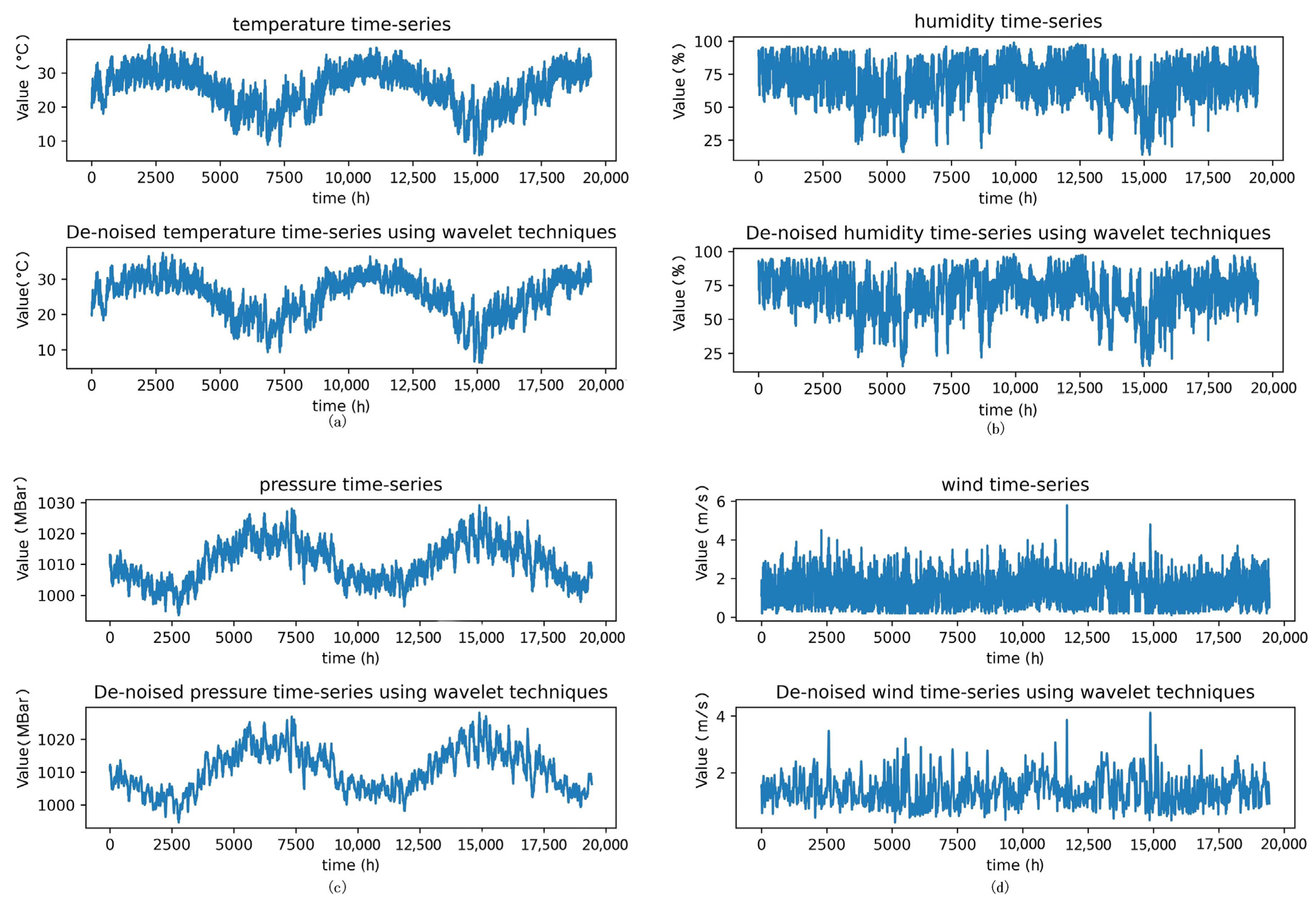
To improve the quality of meteorological data, wavelet transform noise reduction is applied to four time series of temperature, humidity, barometric pressure, and wind speed.
Figure 2 depicts the visualization comparison graph of time series data with noise reduction using the wavelet transform. (a) demonstrates the processing effect of wavelet transform noise reduction for the temperature data, (b) demonstrates the processing effect for the humidity data, (c) demonstrates the processing effect for the pressure data, and (d) demonstrates the processing effect for the wind speed data.
As demonstrated in Figure 2a, the temperature profile reflects a seasonal cycle, and as our data range from April 2019 to July 2021, the change in temperature reflects the seasonal change in the region precisely.
As indicated in Table 1, we utilized the signal-to-noise ratio (SNR) and root mean square error (RMSE) in this research to quantify the fluctuation in data quality, where a larger SNR value and a smaller RMSE indicate a more effective noise reduction.
3.2. DCCA Coefficients on Each Scale and Their Relationship
The window size was divided into three different scales. 0 < n < 1000 denotes a small scale, 1000 < n < 10,000 a medium scale, and n > 10,000 a long scale, for examination and analysis.
Figure 3 depicts the number of DCCA inter-relationships between the AQI index and meteorological variables (temperature, humidity, barometric pressure, and wind speed) for various time frames. The horizontal coordinate represents the time window’s size, with a length of 19,432 h (April 2019 to July 2021). The vertical coordinates represent the DCCA inter-relationship values between −1 and 1, where [−0.2, 0.2] imply no correlation. The yellow line represents the relationship between the AQI and the temperature, the green line represents the relationship between the AQI and the relative humidity, the red line represents the relationship between the AQI and the barometric pressure, and the blue line represents the relationship between the AQI and the wind speed.
3.2.1. AQI Correlation with Temperature
As depicted by the yellow line in Figure 3, the inter-relationship number curve between AQI and temperature was located at [−0.2, 0.2] near the window size n at [1000, 2200], indicating that, at this time, there was a positive correlation between the AQI and the temperature near the window size n < 1000, and a negative correlation between the AQI and the temperature near n > 2200, and the inter-relation number was at n = 12,500 near the minimum value. Overall, there appeared to be a negative link between the AQI and the temperature as the window length increased, i.e., the higher the temperature, the better the air quality.
3.2.2. AQI Correlation with Humidity
As shown by the green lines in Figure 3, almost all of the inter-relationship curves between the AQI and the humidity were negative, indicating that there was a negative correlation between the AQI and the humidity. Furthermore, the inter-relationship curves generally reflected a decreasing and then increasing trend with the change in window size, and the curves reflected a decreasing and then increasing trend in the interval n < 1000. The intercorrelation number between the AQI and the humidity remained above −0.8 after the window size n = 5100, indicating a strong negative correlation.
3.2.3. AQI Correlation with Pressure
The red line in Figure 3 represents the relationship change curve between the AQI and the barometric pressure. The majority of inter-relationships between the AQI and the barometric pressure were positive, demonstrating a positive correlation between the AQI and the barometric pressure, and the A-P coefficient was zero around n = 700.
3.2.4. AQI Correlation with Wind
The blue line in Figure 3 is the inter-relationship number change curve between the AQI and the wind speed. In the graph, the inter-relation number between the AQI and the wind speed was predominantly negative, showing a negative link between AQI and wind speed, and the inter-relation number was stable at −0.68 around n = 16,500.
3.3. DCCA-LSTM Predictive Analysis at Short-Medium and Long Scales
The experiments used the CUDA version of the Pytorch framework to build a multi-input single-output two-layer LSTM model for training and validation, with the following model parameters: the batch size was set to 64, the epoch was set to 20, the training hidden layer size hidden size was set to 128, the forgetting rate drop out was set to 0.2, and patience was set 5; the model was configured to terminate if the loss rate of the validation set did not significantly improve after five consecutive training sessions.
In this article, the previous moment parameters such as AQI, temperature, humidity, barometric pressure, and wind speed were employed as inputs, and AQI values were produced as outputs for the next moment. The model’s accuracy was determined by comparing the output AQI values to the actual AQI values in the dataset.
3.3.1. Short-Scale Application of the DCCA-LSTM Model
This part analyzes, at short scales, the prediction effects of 24 h, 48 h, and 168 h time steps after screening critical inputs with DCCA coefficients, so as to have short-range practical significance.
Table 2 displays the A-T, A-H, A-P, and A-W coefficients at short scales for the 24 h, 48 h, and 168 h windows that were used to filter the model input characteristics. For instance, because the A-W coefficients for the 24 h period and the A-P coefficients for the 48 and 168 h periods were less than −0.2, no wind speed data were entered for the 24 h period, and no barometric pressure data were entered for the 48 and 168 h periods.
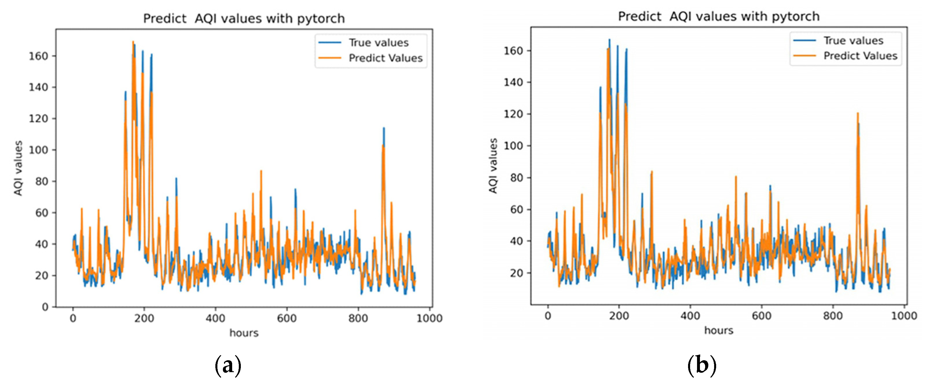
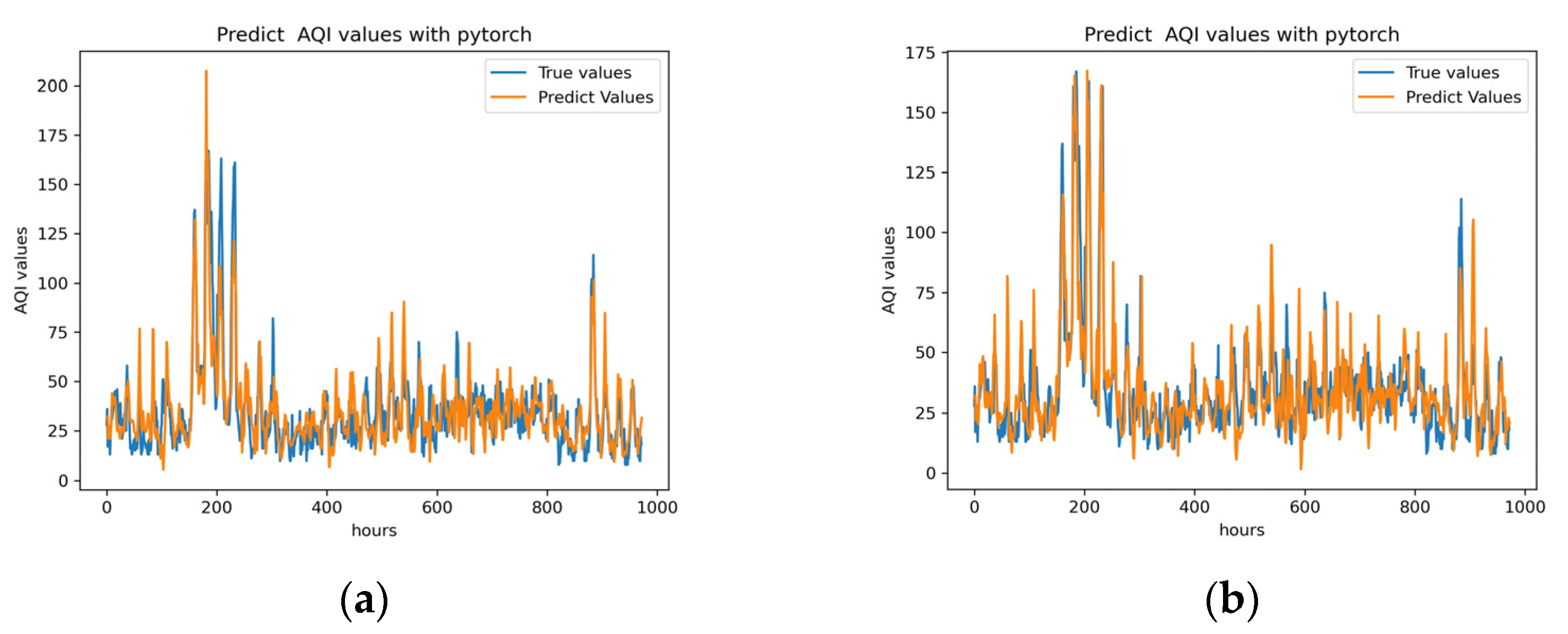
As demonstrated in Figure 4, the LSTM model based on wavelet transform and DCCA correlation coefficients was experimentally plotted against the true and predicted AQI values on the test set; the vertical coordinates represent the AQI values, the horizontal coordinates represent the time series, the solid blue line represents the true sample data values, and the solid orange line represents the predicted values of the model at the next time step.
Figure 4 uses data from the preceding 24 h, or one day, to estimate the AQI value at the following step when the A-W coefficient was less than 0.2. From Table 2, since the A-W coefficient was −0.125, it fell within the interval [−0.2, 0.2], indicating that there was a low correlation between the wind speed data and the AQI representation. Thus, the wind speed data were omitted. Figure 5 uses data from the preceding 48 h or two days to estimate the AQI value at the following moment when the A-P factor was less than 0.2, which was inconsequential, and omits pressure data as a result. Figure 6 uses data from the past 168 h or week to estimate the AQI value at the following instant when the A-P coefficient was equal to −0.09, which was not significant, and omits pressure data.
Using the mean squared error (MSE) to test the model’s correctness, the statistics in Table 3 indicate that the window size equal 24 LSTM model with DCCA coefficients to filter the variables reduced the mean squared error by around 0.01 and improved the running time by approximately 1 s. When the window size was 48, the mean square error decreased by 0.016 and the efficiency increased by 2 s. When the window length was 168, the mean square error decreased by 0.02 and the efficiency increased by 4 s.
3.3.2. Medium-Scale and Long-Scale Application of the DCCA-LSTM Model
When the length of the window fell within the medium–long scale, all climatic characteristics were significantly connected with the AQI. Here, the DCCA coefficient was chosen as the weighting factor to quantify the relevance of the feature when the window length was 5000, and the prediction results are displayed in Figure 7 and Table 4.
Since both the AQI and variable characteristics exhibited correlation features at the medium and long scales, variable screening was not practicable; thus, DCCA coefficients were added into the LSTM model as weighting factors, which improved the accuracy by 5% and the running time by 22 s.
4. Discussion
Using DCCA correlation coefficients, the correlation analysis of air quality achieves quantification at several scales. It facilitates multidimensional feature meritocracy in time series prediction, which minimizes the amount of input data for the prediction model while ensuring accuracy, and it gives a means to incorporate feature weighting parameters in the model, which helps to increase prediction accuracy. The research can be expanded to incorporate models with more complex characteristics, and the model can be paired with an attention mechanism to give weighting factors to multidimensional features, improving the prediction model’s accuracy.
5. Conclusions
In this study, we first used air pollution elements (SO2, NO2, PM10, PM2.5, O3, and CO) to calculate the air quality index to quantify the air pollution level, then used wavelet transform noise reduction to optimize the data quality of meteorological indicators (temperature, humidity, barometric pressure, and wind speed), and finally used the detrended correlation analysis (DCCA) technique to calculate the detrended correlation number DCCA to evaluate the correlation between air pollution and meteorological variables, representing the development of a DCCA-LSTM model that successfully filters and preserves changed information at short scales. Using DCCA as a variable weighting factor enhanced the multivariate single-step prediction accuracy of air pollution AQI values at three scales at medium and long scales.
The DCCA-LSTM model was then used to compare the multivariate single-step prediction effects with those of the LSTM model. The simulation plots, mean squared errors, and running times demonstrated that the accuracy of the prediction model improved by 1%, 1.6%, 2%, and 5% on the short, medium, and long scales with window sizes of 24, 48, 168, and 5000 h, respectively, and that the efficiency improved by 5.72%, 8.64%, 8.29%, and 3.42%, indicating the DCCA-LSTM model derived by the DCCA correlation analysis was effective and efficient for the multivariate single-step prediction of air pollution index variables.
Author Contributions
Conceptualization, X.H.; methodology, software, Z.Z.; validation, formal analysis, H.C.; writing—original draft preparation, writing—review and editing, Z.Z.; All authors have read and agreed to the published version of the manuscript.
Funding
This research was funded by the Key Project of the Application Foundation of Sichuan Science and Technology Department, China, grant number 2019YJ0455 and the Graduate Innovation Fund of Xihua University, China, grant number YCJJ2021072.
Institutional Review Board Statement
Not applicable.
Informed Consent Statement
Not applicable.
Data Availability Statement
On behalf of all the authors, the corresponding author states that our data are available upon reasonable request.
Acknowledgments
We express our gratitude to the management of the School of Electrical and Electronic Information at Xihua University for providing us with the necessary support and research facilities to complete this work.
Conflicts of Interest
The authors declare no conflict of interest.
References
- Lu, X.; Zhang, S.; Xing, J.; Wang, Y.; Chen, W.; Ding, D.; Wu, Y.; Wang, S.; Duan, L.; Hao, J. Progress of air pollution control in china and its challenges and opportunities in the ecological civilization era. Engineering 2020, 6, 1423–1431. [Google Scholar] [CrossRef]
- Haq, M.A. Smotednn: A novel model for air pollution forecasting and aqi classification. Comput. Mater. Contin. 2022, 71, 1403–1425. [Google Scholar]
- Xu, K.; Cui, K.; Young, L.-H.; Wang, Y.-F.; Hsieh, Y.-K.; Wan, S.; Zhang, J. Air quality index, indicatory air pollutants and impact of COVID-19 event on the air quality near central China. Aerosol Air Qual. Res. 2020, 20, 1204–1221. [Google Scholar] [CrossRef] [Green Version]
- Yates, E.F.; Zhang, K.; Naus, A.; Forbes, C.; Wu, X.; Dey, T. A Review on the Biological, Epidemiological, and Statistical Relevance of COVID-19 Paired with Air Pollution. Environ. Adv. 2022, 8, 100250. [Google Scholar] [CrossRef]
- Huang, X.L.; Hu, S.Y.; Chen, J.X.; Feng, W.Q. Air quality analysis of Sichuan province based on complex network and CSP algorithm. Int. J. Mod. Phys. C 2021, 33, 2250007. [Google Scholar] [CrossRef]
- Xu, H.; Croot, P.; Zhang, C. Exploration of the spatially varying relationships between lead and aluminium concentrations in the topsoil of northern half of Ireland using Geographically Weighted Pearson Correlation Coefficient. Geoderma 2022, 409, 115640. [Google Scholar] [CrossRef]
- Zhang, J.; Li, Y.; Liu, C.; Wu, B.; Shi, K. A study of cross-correlations between PM2.5 and O3 based on Copula and Multifractal methods. Phys. A Stat. Mech. Its Appl. 2022, 589, 126651. [Google Scholar] [CrossRef]
- Kojić, M.; Schlüter, S.; Mitić, P.; Hanić, A. Economy-environment nexus in developed European countries: Evidence from multifractal and wavelet analysis. Chaos Solitons Fractals 2022, 160, 112189. [Google Scholar] [CrossRef]
- Méndez-Figueroa, H.; Colorado-Garrido, D.; Hernández-Pérez, M.; Galván-Martínez, R.; Cruz, R.O. Neural networks and correlation analysis to improve the corrosion prediction of SiO2-nanostructured patinated bronze in marine atmospheres. J. Electroanal. Chem. 2022, 917, 116396. [Google Scholar] [CrossRef]
- Du, Z.; Lawrence, W.R.; Zhang, W.; Zhang, D.; Yu, S.; Hao, Y. Interactions between climate factors and air pollution on daily HFMD cases: A time series study in Guangdong, China. Sci. Total. Environ. 2019, 656, 1358–1364. [Google Scholar] [CrossRef]
- Shen, C.-H.; Li, C.-L.; Si, Y.-L. A detrended cross-correlation analysis of meteorological and API data in Nanjing, China. Phys. A: Stat. Mech. Its Appl. 2015, 419, 417–428. [Google Scholar] [CrossRef]
- Zebende, G.F.; Brito, A.A.; Castro, A.P. DCCA cross-correlation analysis in time-series with removed parts. Phys. A Stat. Mech. Its Appl. 2020, 545, 123472. [Google Scholar] [CrossRef]
- Pavlov, A.; Pavlova, O.; Koronovskii, A.; Guyo, G. Extended detrended cross-correlation analysis of nonstationary processes. Chaos Solitons Fractals 2022, 157, 111972. [Google Scholar] [CrossRef]
- Ben-Salha, O.; Mokni, K. Detrended cross-correlation analysis in quantiles between oil price and the US stock market. Energy 2022, 242, 122918. [Google Scholar] [CrossRef]
- Chen, J.; Shi, Z.; Li, W.; Guo, Y. Bidirectional lstm-crf attention-based model for chinese word segmentation. arXiv 2021, arXiv:2105.09681. [Google Scholar]
- Atila, O.; Şengür, A. Attention guided 3D CNN-LSTM model for accurate speech based emotion recognition. Appl. Acoust. 2021, 182, 108260. [Google Scholar] [CrossRef]
- Pathak, B.; Mittal, S.; Shinde, K.; Pawar, P. Comparison Between LSTM and RNN Algorithm for Speech-to-Speech Translator. Proceedings of International Conference on Communication, Circuits, and Systems, Washington, DC, USA, 6–9 June 2021; Springer: Singapore, 2021. [Google Scholar]
- Aslan, S.N.; Özalp, R.; Uçar, A.; Güzeliş, C. New CNN and hybrid CNN-LSTM models for learning object manipulation of humanoid robots from demonstration. Clust. Comput. 2022, 25, 1575–1590. [Google Scholar] [CrossRef]
- Ouma, Y.O.; Cheruyot, R.; Wachera, A.N. Rainfall and runoff time-series trend analysis using LSTM recurrent neural network and wavelet neural network with satellite-based meteorological data: Case study of Nzoia hydrologic basin. Complex Intell. Syst. 2022, 8, 213–236. [Google Scholar] [CrossRef]
- Shastri, S.; Singh, K.; Kumar, S.; Kour, P.; Mansotra, V. Deep-LSTM ensemble framework to forecast COVID-19: An insight to the global pandemic. Int. J. Inf. Technol. 2021, 13, 1291–1301. [Google Scholar] [CrossRef]
- Shen, Z.; Fan, X.; Zhang, L.; Yu, H. Wind speed prediction of unmanned sailboat based on CNN and LSTM hybrid neural network. Ocean Eng. 2022, 254, 111352. [Google Scholar] [CrossRef]
- Xiang, L.; Liu, J.; Yang, X.; Hu, A.; Su, H. Ultra-short term wind power prediction applying a novel model named SATCN-LSTM. Energy Convers. Manag. 2022, 252, 115036. [Google Scholar] [CrossRef]
- Haq, M.A. CDLSTM: A Novel Model for Climate Change Forecasting. Comput. Mater. Contin. 2022, 71, 2363–2381. [Google Scholar] [CrossRef]
- He, J.; Cui, J.; Zhang, G.; Xue, M.; Chu, D.; Zhao, Y. Spatial–temporal seizure detection with graph attention network and bi-directional LSTM architecture. Biomed. Signal Process. Control. 2022, 78, 103908. [Google Scholar] [CrossRef]
- Panja, P.; Jia, W.; McPherson, B. Prediction of Well Performance in SACROC Field Using Stacked Long Short-Term Memory (LSTM) Network. Expert Syst. Appl. 2022, 205, 117670. [Google Scholar] [CrossRef]
- Haq, M.A.; Jilani, A.K.; Prabu, P. Deep learning based modeling of groundwater storage change. Comput. Mater. Contin. 2021, 70, 4599–4617. [Google Scholar] [CrossRef]
- Rhif, M.; Ben Abbes, A.; Farah, I.R.; Martínez, B.; Sang, Y. Wavelet transform application for/in non-stationary time-series analysis: A review. Appl. Sci. 2019, 9, 1345. [Google Scholar] [CrossRef] [Green Version]
- Shen, C.-H.; Li, C.-L. An analysis of the intrinsic cross-correlations between API and meteorological elements using DPCCA. Phys. A Stat. Mech. Its Appl. 2016, 446, 100–109. [Google Scholar] [CrossRef]
- Yu, Y.; Si, X.; Hu, C.; Zhang, J. A review of recurrent neural networks: LSTM cells and network architectures. Neural Comput. 2019, 31, 1235–1270. [Google Scholar] [CrossRef]
Figure 1.
LSTM cell structure diagram.

Figure 2.
Temperature Feature Reconstruction (a). Humidity Feature Reconstruction (b). Pressure Feature Reconstruction (c). Wind Feature Reconstruction (d).
Figure 2.
Temperature Feature Reconstruction (a). Humidity Feature Reconstruction (b). Pressure Feature Reconstruction (c). Wind Feature Reconstruction (d).

Figure 3.
The inter-relationship curves of AQI with temperature, humidity, air pressure, and wind speed are color-coded. Blue represents the coefficient between AQI and wind speed, red represents the coefficient between AQI and air pressure, green represents the coefficient between AQI and humidity, and yellow represents the coefficient between AQI and temperature.

Figure 4.
24 h comparison of forecasts. (a) Results of prediction without DCCA feature screening. (b) Prediction outcomes following DCCA feature screening.
Figure 4.
24 h comparison of forecasts. (a) Results of prediction without DCCA feature screening. (b) Prediction outcomes following DCCA feature screening.

Figure 5.
48 h comparison of forecasts. (a) Results of prediction without DCCA feature screening. (b) Prediction outcomes following DCCA feature screening.
Figure 5.
48 h comparison of forecasts. (a) Results of prediction without DCCA feature screening. (b) Prediction outcomes following DCCA feature screening.

Figure 6.
168 h comparison of forecasts. (a) Results of prediction without DCCA feature screening. (b) Prediction outcomes following DCCA feature screening.
Figure 6.
168 h comparison of forecasts. (a) Results of prediction without DCCA feature screening. (b) Prediction outcomes following DCCA feature screening.

Figure 7.
5000 h comparison of forecasts. (a) Results of prediction without DCCA factor weighting. (b) Prediction outcomes following DCCA factor weighting.
Figure 7.
5000 h comparison of forecasts. (a) Results of prediction without DCCA factor weighting. (b) Prediction outcomes following DCCA factor weighting.


Table 1.
Quality indicator of time series following noise reduction by means of wavelet transform.
| Features | SNR | RMSE |
|---|---|---|
| Temperature | 30.087368 | 0.802346 |
| Humidity | 29.952903 | 1.256670 |
| Pressure | 62.939602 | 0.720441 |
| Wind | 10.224503 | 0.452248 |
Table 2.
DCCA coefficients for 24 h, 48 h and 168 h windows at short time series scales.
| Window-Size | A-T | A-H | A-P | A-W |
|---|---|---|---|---|
| 24 | 0.638617 | −0.600959 | −0.240827 | −0.125029 |
| 48 | 0.519856 | −0.396133 | −0.170982 | −0.281052 |
| 168 | 0.365726 | −0.24658 | −0.095371 | −0.503246 |
Table 3.
Model performance parameters for short scales with window lengths of 24, 48, and 168.
| Window | Model | Train Loss | Valid Loss | MSE | Time(s) |
|---|---|---|---|---|---|
| 24 | LSTM | 0.052742 | 0.049323 | 0.08974096 | 17.0574 |
| DCCA-LSTM | 0.049790 | 0.047054 | 0.08095255 | 16.0810 | |
| 48 | LSTM | 0.034793 | 0.032198 | 0.13867431 | 21.3187 |
| DCCA-LSTM | 0.033351 | 0.030843 | 0.12241591 | 19.4778 | |
| 168 | LSTM | 0.018447 | 0.015060 | 0.15315998 | 41.0941 |
| DCCA-LSTM | 0.017658 | 0.014200 | 0.13412123 | 37.6885 |
Table 4.
Model performance parameters for medium and long scale with window lengths of 5000.
| Window | Model | Train Loss | Valid Loss | MSE | Time(s) |
|---|---|---|---|---|---|
| 5000 | LSTM | 0.009910 | 0.006814 | 0.2568583 | 662.7335 |
| DCCA-LSTM | 0.008748 | 0.005752 | 0.2008781 | 640.0185 |
Disclaimer/Publisher’s Note: The statements, opinions and data contained in all publications are solely those of the individual author(s) and contributor(s) and not of MDPI and/or the editor(s). MDPI and/or the editor(s) disclaim responsibility for any injury to people or property resulting from any ideas, methods, instructions or products referred to in the content. |
© 2023 by the authors. Licensee MDPI, Basel, Switzerland. This article is an open access article distributed under the terms and conditions of the Creative Commons Attribution (CC BY) license (https://creativecommons.org/licenses/by/4.0/).
Share and Cite
MDPI and ACS Style
Zhang, Z.; Chen, H.; Huang, X. Prediction of Air Quality Combining Wavelet Transform, DCCA Correlation Analysis and LSTM Model. Appl. Sci. 2023, 13, 2796. https://0-doi-org.brum.beds.ac.uk/10.3390/app13052796
AMA Style
Zhang Z, Chen H, Huang X. Prediction of Air Quality Combining Wavelet Transform, DCCA Correlation Analysis and LSTM Model. Applied Sciences. 2023; 13(5):2796. https://0-doi-org.brum.beds.ac.uk/10.3390/app13052796
Chicago/Turabian StyleZhang, Zheng, Haibo Chen, and Xiaoli Huang. 2023. "Prediction of Air Quality Combining Wavelet Transform, DCCA Correlation Analysis and LSTM Model" Applied Sciences 13, no. 5: 2796. https://0-doi-org.brum.beds.ac.uk/10.3390/app13052796
Note that from the first issue of 2016, this journal uses article numbers instead of page numbers. See further details here.