
Seismic Periodic Noise Attenuation Based on Sparse Representation Using a Noise Dictionary


1
SINOPEC Research Institute of Petroleum Engineering Co., Ltd., Beijing 102206, China
2
School of Geophysics and Information Technology, China University of Geosciences, Beijing 100083, China
3
The State Key Laboratory of Ore Deposit Geochemistry, Institute of Geochemistry, Chinese Academy of Sciences, Guiyang 550081, China
*
Author to whom correspondence should be addressed.
Appl. Sci. 2023, 13(5), 2835; https://0-doi-org.brum.beds.ac.uk/10.3390/app13052835
Submission received: 15 January 2023
/
Revised: 18 February 2023
/
Accepted: 19 February 2023
/
Published: 22 February 2023
(This article belongs to the Special Issue Technological Advances in Seismic Data Processing and Imaging)
Abstract
:Periodic noise is a well-known problem in seismic exploration, caused by power lines, pump jacks, engine operation, or other interferences. It contaminates seismic data and affects subsequent processing and interpretation. The conventional methods to attenuate periodic noise are notch filtering and some model-based methods. However, these methods either simultaneously attenuate noise and seismic events around the same frequencies, or need expensive computation time. In this work, a new method is proposed to attenuate periodic noise based on sparse representation. We use a noise dictionary to sparsely represent periodic noise. The noise dictionary is constructed based on ambient noise. An advantage of our method is that it can automatically suppress monochromatic periodic noise, multitoned periodic noise and even periodic noise with complex waveforms without pre-known noise frequencies. In addition, the method does not result in any notches in the spectrum. Synthetic and field examples demonstrate that our method can effectively subtract periodic noise from raw seismic data without damaging the useful seismic signal.
1. Introduction
Noise decreases the signal-to-noise ratio (SNR) of seismic data and affects the quality of subsequent processes [1,2]. There are six types of noise recorded using geophones [3], in which periodic noise is a kind of noise caused by power lines, pump jacks [4], engine operation [5], or other interferences, shown as monochromatic noise or multitoned noise. Sometimes, periodic noise is so strong that seismic records are severely contaminated. However, it is not easy to attenuate periodic noise, since it overlaps with seismic waves in the time domain and the frequency domain.
For periodically monochromatic noise, the conventional method of attenuation is notch filtering, which requires exact knowledge of the frequency of monochromatic noise [6]. Obviously, the notch filtering method can attenuate seismic waves at the cutoff frequency. Model-based approaches [7,8,9,10] such as sinusoidal approximation are used to remove power line noise, though this method requires accurate estimation of noise frequency and needs significant computation time [11]. Henley [12] presented a spectral clipping method to detect monochromatic noise automatically; however, it is not applicable to weak periodic noise. Karsli and Dondurur [13] used an improved mean filtering method to attenuate power line harmonic noise without noise frequency estimation; however, this requires knowledge of the rough frequency band.
In recent years, following the application of wide-azimuth, broadband, high-density seismic acquisition technology—including micro-seismic observation [14] and time-lapse monitoring based on fiber sensing—the size of 3D seismic data is increasing, and the frequency band of reflections is becoming wider. Besides monochromatic noises suppression, recognition of multitoned noises and their automatic suppression are urgently needed. Methods based on sparsity representation, such as S-transform, singular spectrum analysis and empirical mode decomposition, extend realization of automatic denoising [15,16,17]. Xu et al. [4] proposed a method based on morphological diversity of monochromatic noise and seismic waves, which assumed that the raw data are only composed of two kinds of signals, the monochromatic noise and seismic waves. It is not applicable to seismic data with strong white Gaussian noise or multitoned noise.
In this paper, a new method is proposed to attenuate periodic noise. The proposed method is based on sparse representation using a noise dictionary. The novelty is the construction of a noise dictionary, which can represent periodic noise sparsely. First, the noise dictionary is constructed using ambient noise. Next, the noise dictionary is used to sparsely represent periodic noise. Then, the de-noised data are obtained by subtracting the periodic noise from the raw seismic data. The method is applied to synthetic and field seismic data. The effectiveness of the proposed method is that it can subtract periodic noise from raw seismic data without any notches in the spectrum compared with the notch filtering method.
2. Method
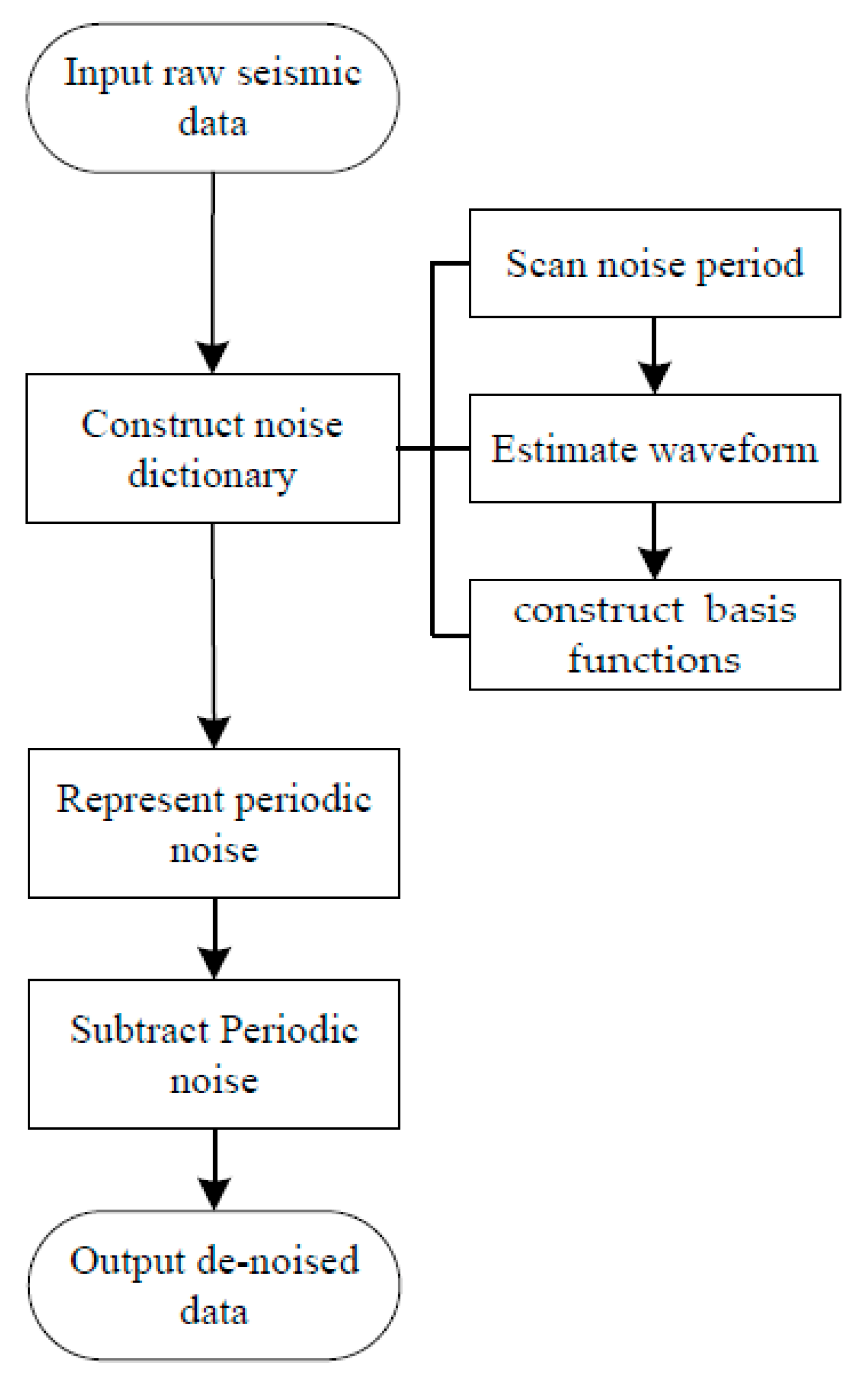
Periodic noise is recurring in raw seismic data, and its amplitude is constant within the recording time [6]. Based on these characteristics, we can differentiate and estimate periodic noise from ambient noise. Because ambient noise, such as periodic noise, white Gaussian noise and other non-stationary [1,18] random noise, is ubiquitous in seismic records before the first arrivals, we can extract noise features and construct the noise dictionary from it. The algorithm is outlined in the flow skeleton (Figure 1).
2.1. Noise Period Scanning
The waveform of periodic noise is similar in a single trace. Based on the similarity, we scan the noise period from ambient noise, which exists in the records before the first arrivals. First, given the scanned period interval , the noise period is changed from the initial scanned period to the final scanned period . The data on the single trace are split into many time windows , denoted as
where the length of time window is equal to the scanned period . The size of is (). Next, the correlation coefficients for the adjacent two time windows and are calculated:
where is the covariance of the two time windows and is the variance of . For accuracy, we average the correlation coefficients to obtain a coefficient to evaluate the similarity of all time windows.
Then, the scanned period is increased and the former procedures are repeated until all periods in the interval are scanned. The period which matches the maximum value of the correlation coefficients is our estimated period:
where is the period of periodic noise on the trace .
2.2. Waveform Estimation by Stacking
The time window, whose length is , is chosen and is represented as . The chosen time window is approximated as the noise waveform; however, it is affected by white Gaussian noise. A stacking method is widely used to improve the SNR of the seismic profile [19], because it weakens white Gaussian noise and emphasizes seismic waves. We stack the approximate waveforms for an accurate noise waveform:
where is the noise waveform on the trace and its length is equal to that of . The waveforms of different traces are similar to the near traces when the traces are interfered with by the same noise source. Therefore, we can stack the similar waveforms along different traces:
where is the noise waveform estimated from the traces . We note that waveforms obtained by Equation (5) are not in phase. Before stacking, waveforms need to be cyclically shifted to the same phase as by scanning the shift length in an interval . The suitable shift length corresponds to the maximum correlation coefficient between and .
2.3. Periodic Noise Representation
Based on the stationarity of periodic noise, the basis function of periodic noise is obtained by extending the waveform iteratively to the length of seismic data on a single trace and then energy-normalized:
where is the norm. The size of is , which is equal to that of . The noise dictionary is constructed by basis functions of different phases:
where are obtained by cyclically shifting time samples. The size of is . The dictionary provides a sparse representation of periodic noise. In sparse representation theory [20], the signals can be efficiently explained as linear combinations of prespecified basis functions, where the linear coefficients are sparse. Based on sparse representation theory, the mathematical model of our noise representation is
where is the actual periodic noise and is its coefficient represented by the dictionary . The size of is . An approach to solve Equation (10) is using the sparsity constraint via an regularization term. Then, the periodic noise of multi-trace seismic data is obtained by solving the following optimization problem:
where is the approximate periodic noise and is its coefficient represented by the dictionary . In the optimization problem, the sparsity of this representation is 1. Because only one basis function corresponds to a single trace, the coefficient has only one non-zero component. This is the reason for the condition on the right in Equation (11) . Equation (11) is solved by the matching pursuit algorithm, which entails computing the inner products between the residual and the dictionary elements, updating the coefficient, and updating the residual iteratively [20,21]. Finally, the de-noised data are obtained by subtracting the periodic noise from the raw seismic data.
3. Synthetic Example
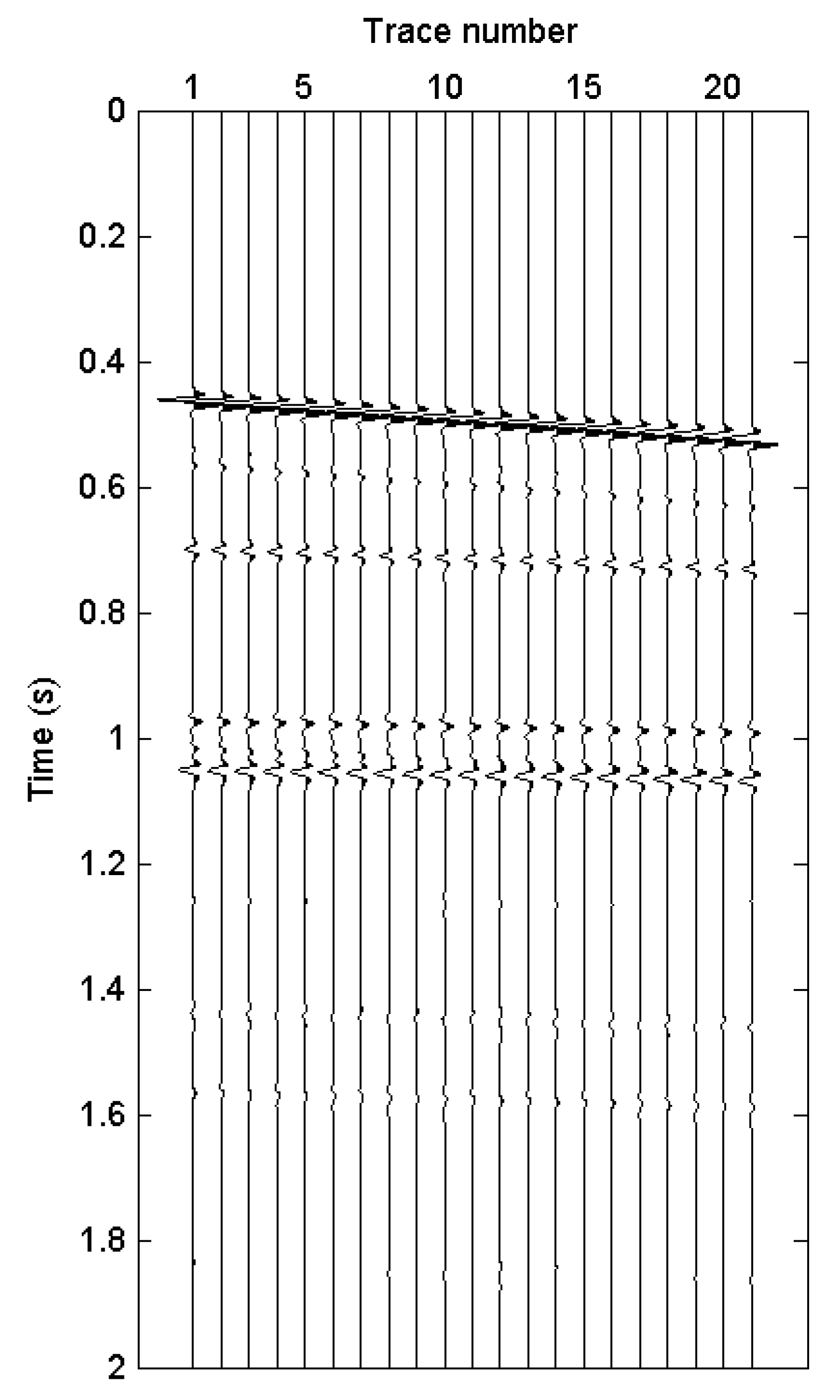
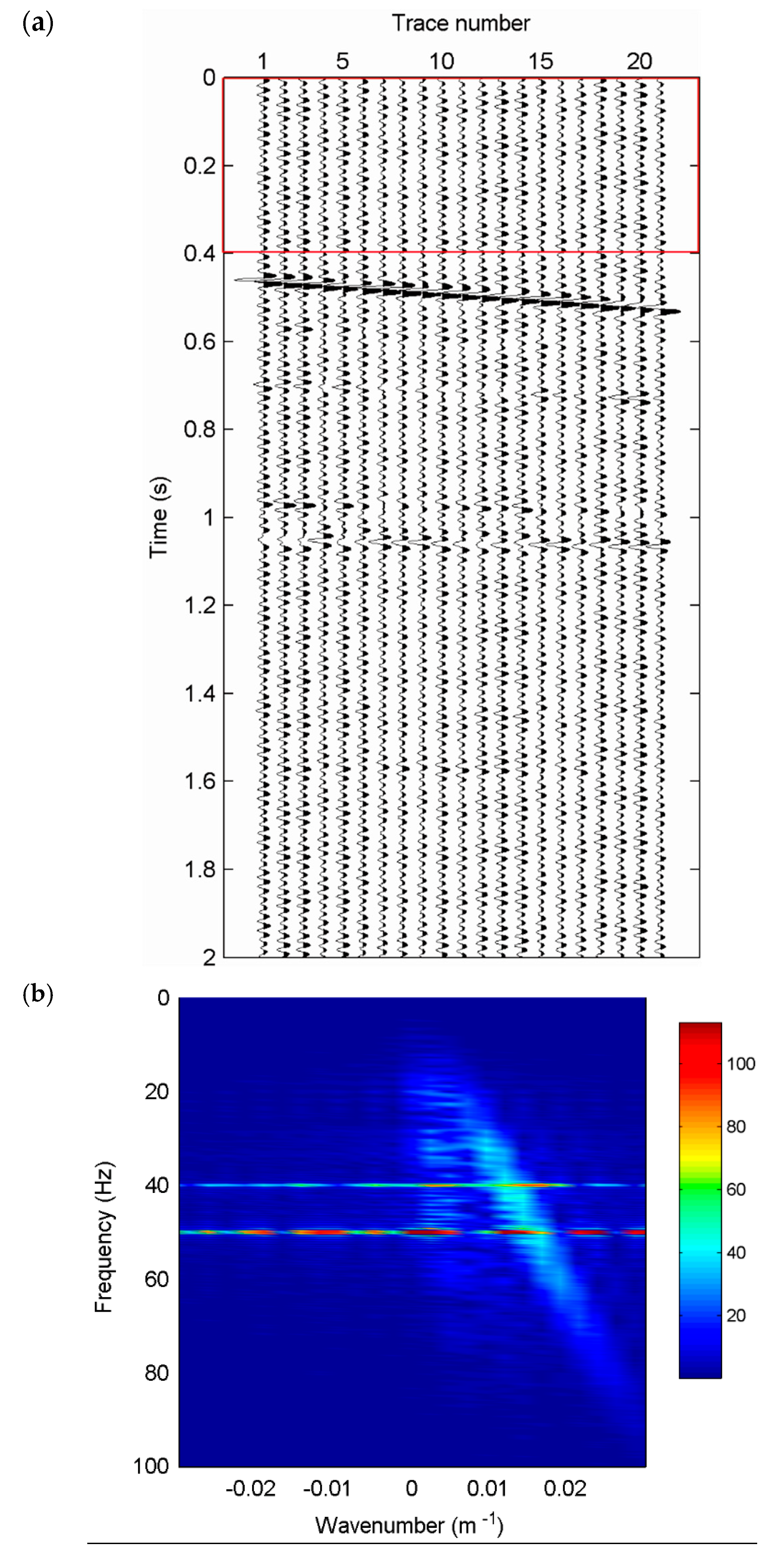
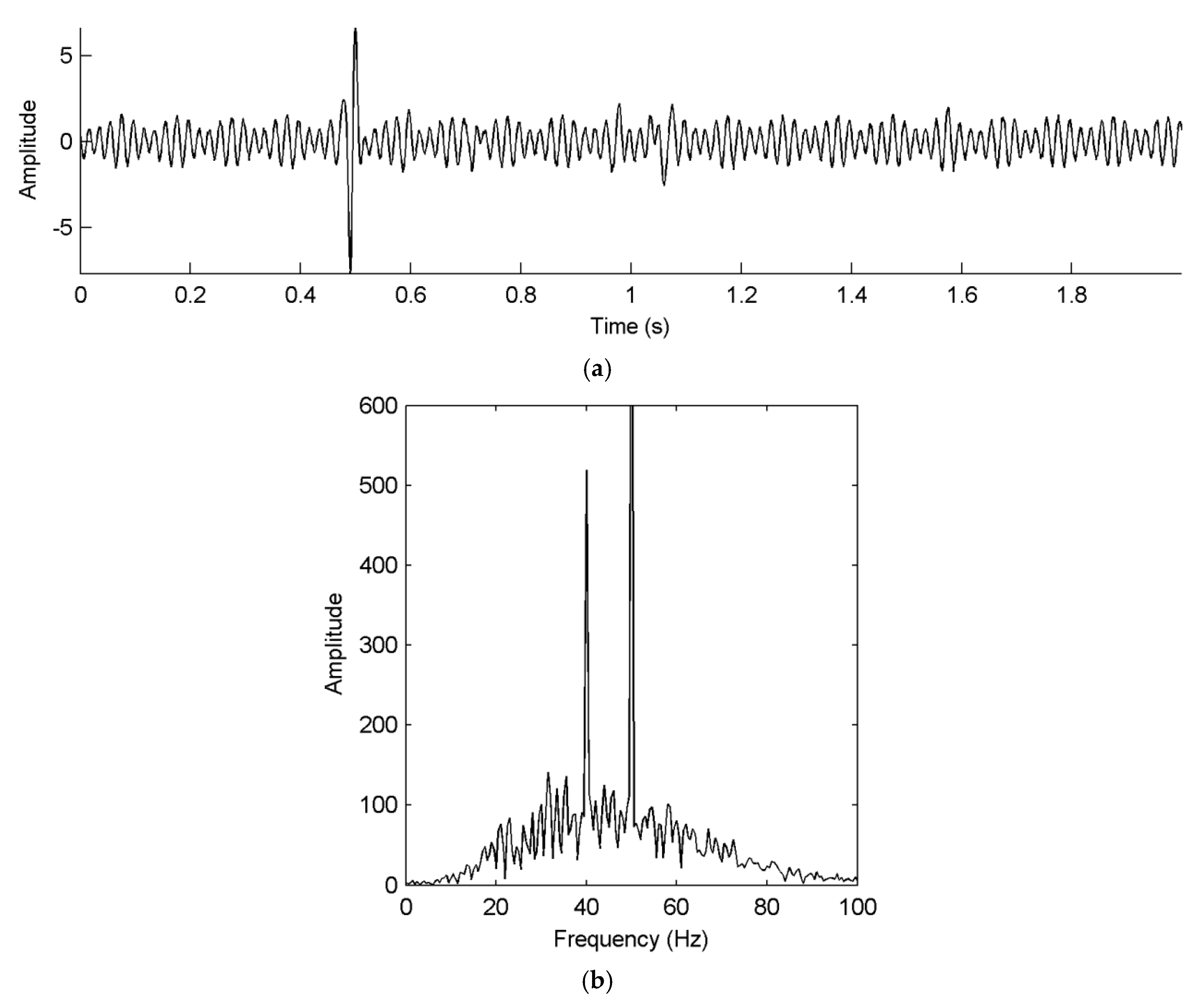
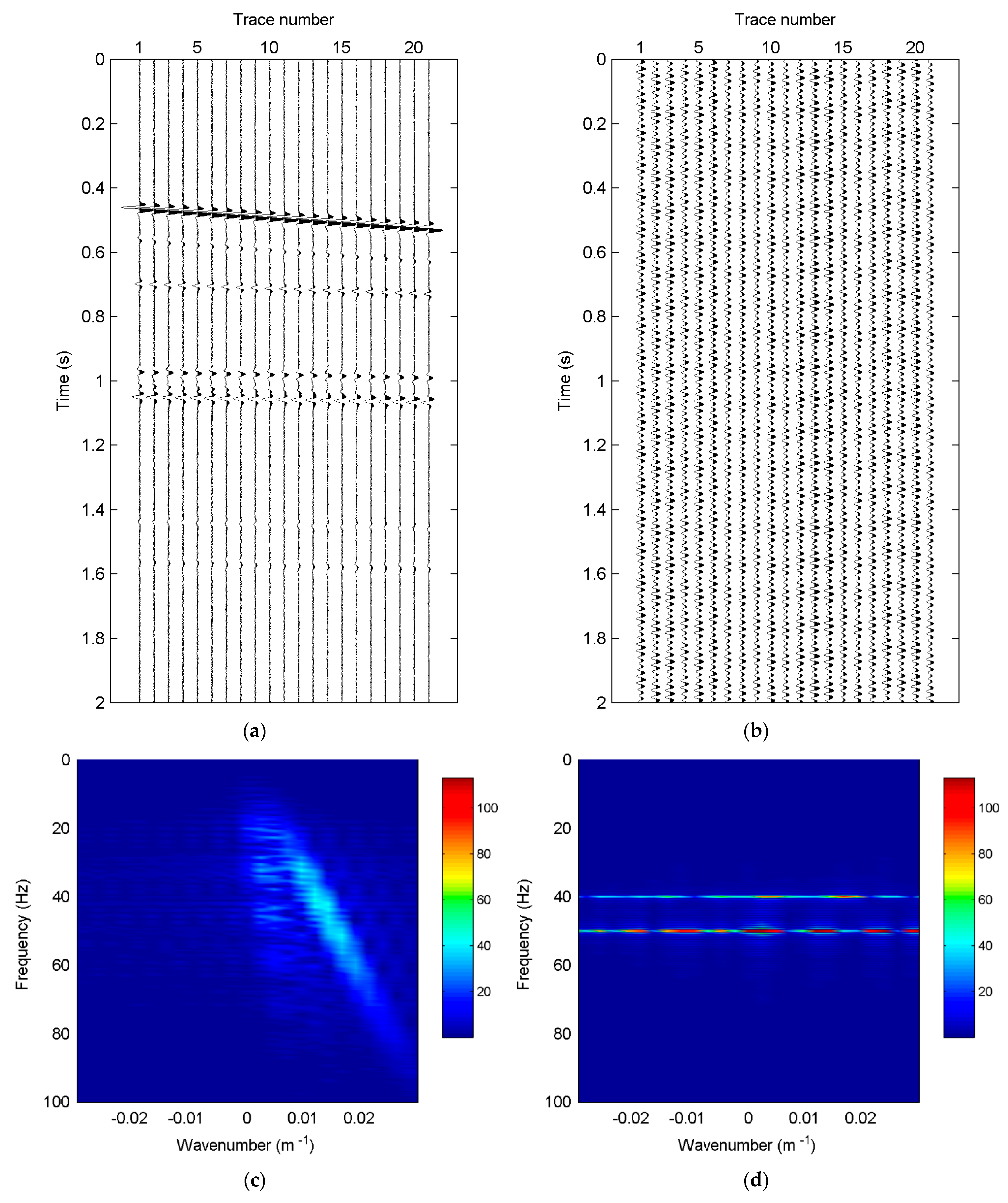
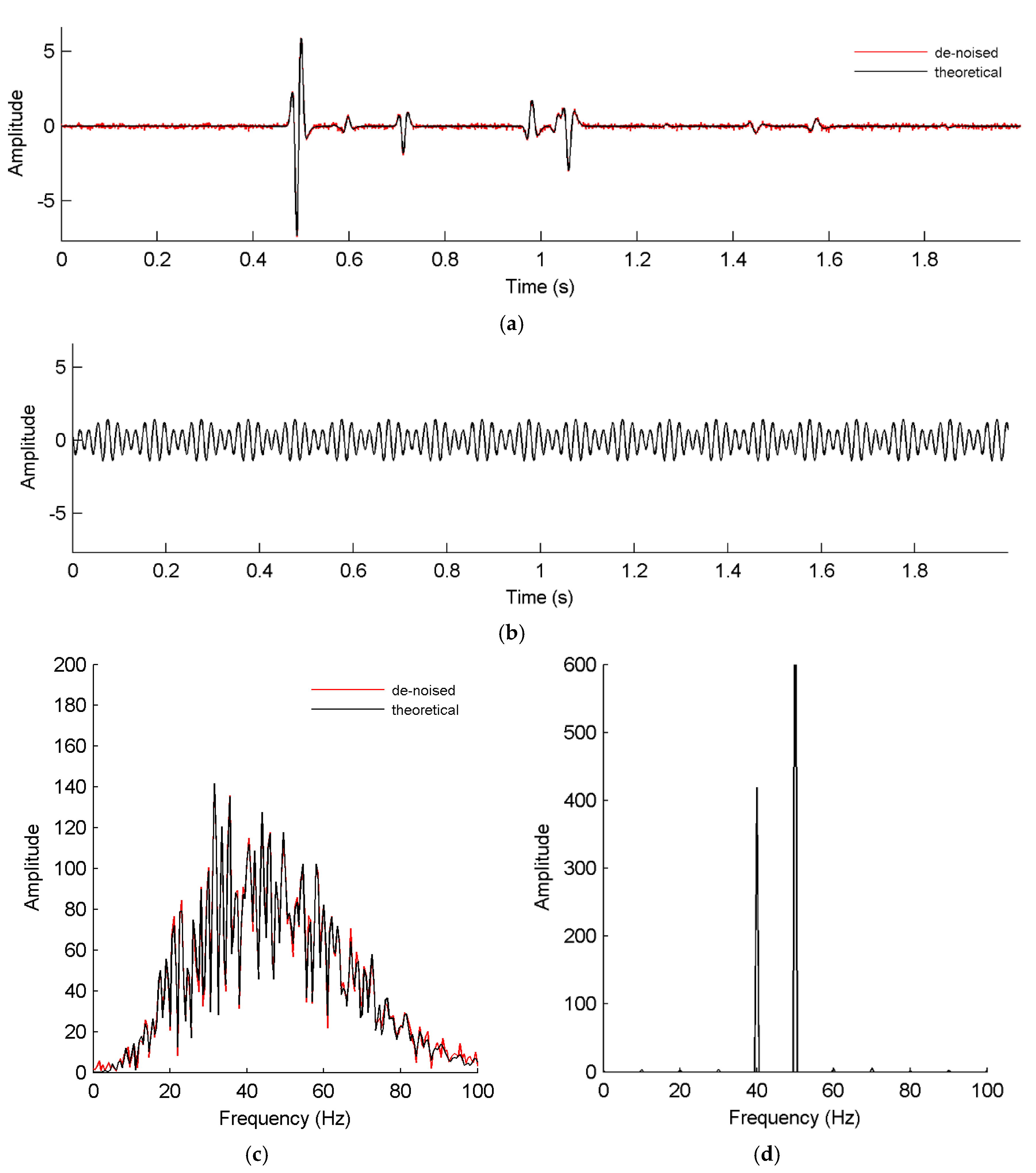
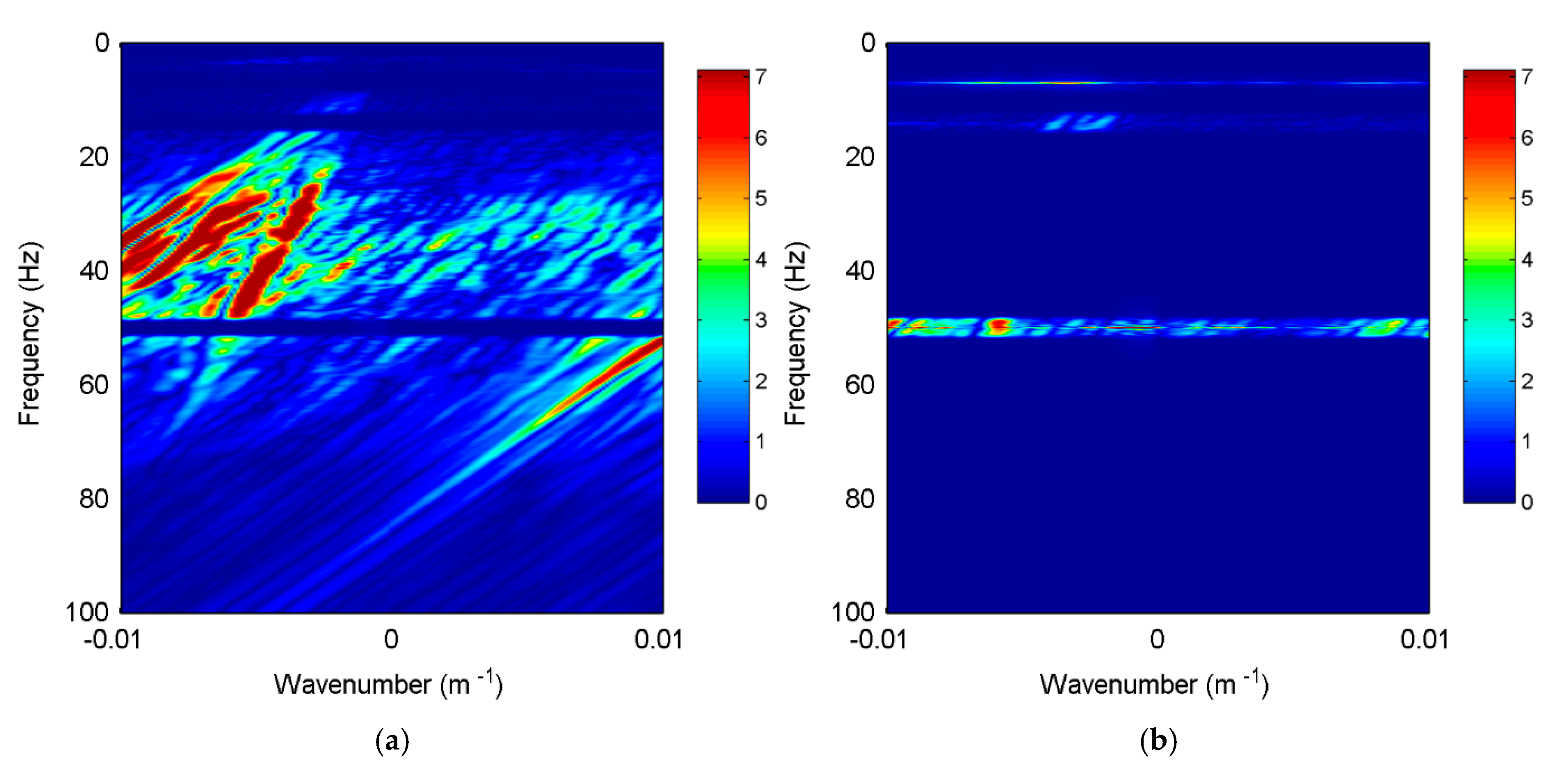
A synthetic dataset consisting of 21 traces is shown in Figure 2 with a 1 ms sampling rate and a 10 m geophone interval. Multitoned noises of 40 Hz and 50 Hz are incorporated to the noise-free data. In addition, a small amount of white Gaussian noise is added. Figure 3 shows the contaminated seismic dataset and its frequency–wavenumber (f-k) spectrum. The reflections are hardly identifiable owing to the strong periodic noise. The contaminations in the seismic data appear as two horizontal bands at 40 and 50 Hz in the f-k domain. The signal on the 11th trace (Figure 4a) shows the influence of multitoned noise clearly. Its amplitude spectrum (Figure 4b) also shows high spikes at frequencies of 40 Hz and 50 Hz.
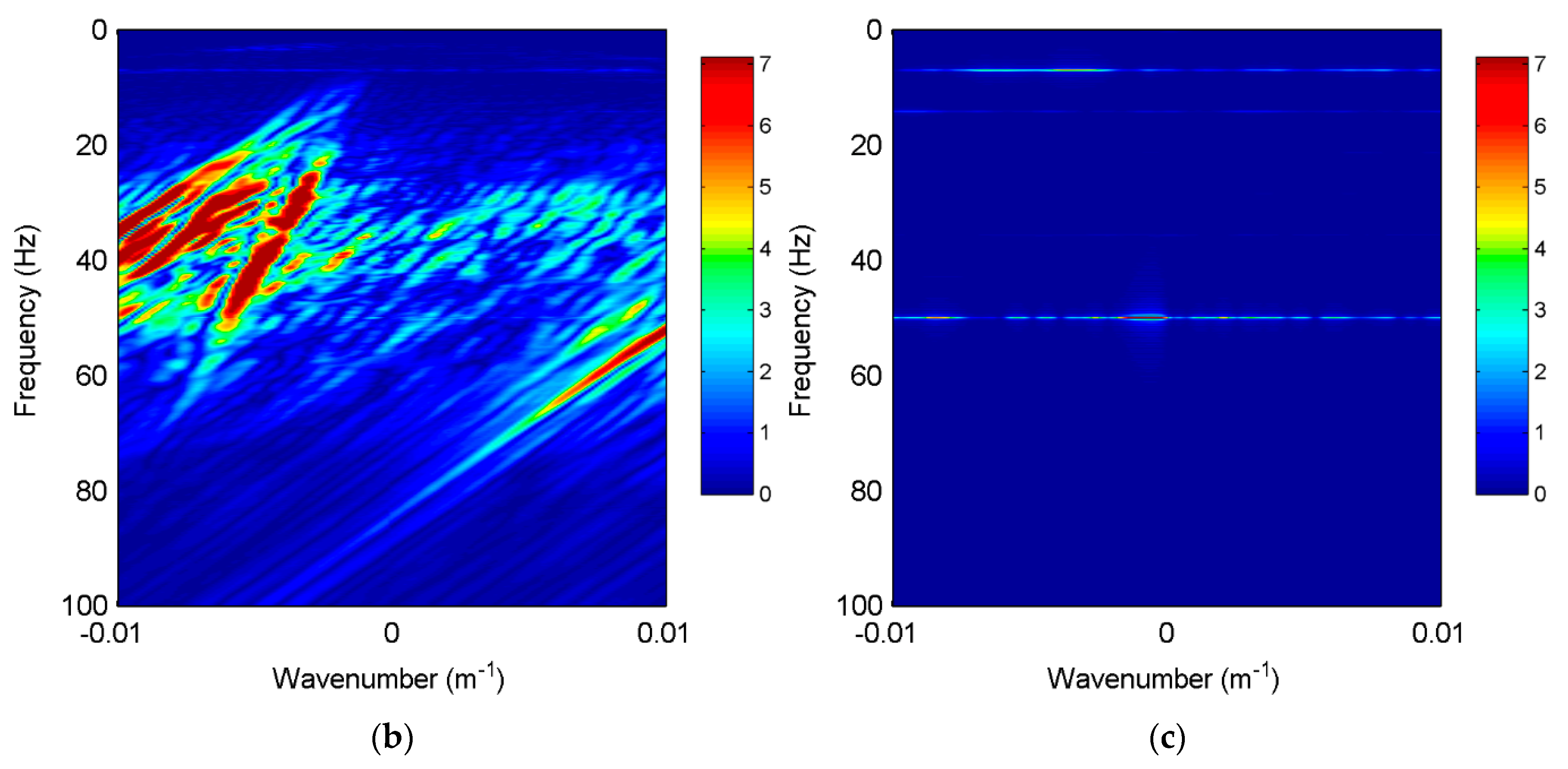
The first 0.4 s of data is dominated by periodic noise marked by a red rectangle in Figure 3a. In addition, it does not consist of seismic waves. Therefore, it is chosen to construct the noise dictionary. The waveform estimated from the chosen data is shown in Figure 5. After sparse representation, the result of noise attenuation is shown in Figure 6. The main noise is attenuated and reflections can be clearly seen in Figure 6a. The eliminated noise is periodic noise as shown in Figure 6b. Their spectra show that the multitoned noise is attenuated and no seismic waves are eliminated. The de-noising result on the 11th trace and the corresponding amplitude spectra are shown in Figure 7. The de-noised seismic signal is close to the theoretical signal in both time sequence and amplitude spectrum, except for weak white Gaussian noise.
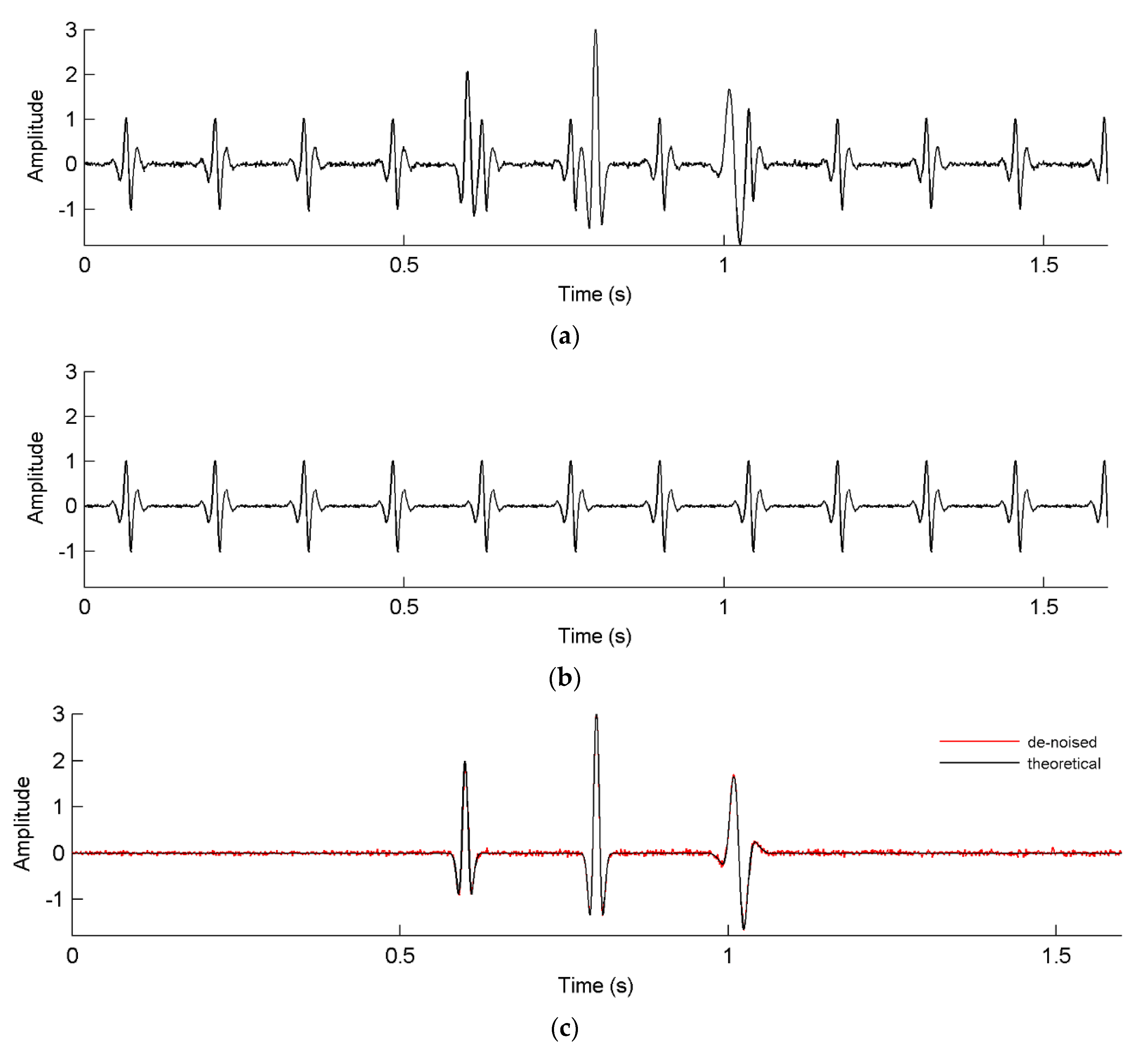
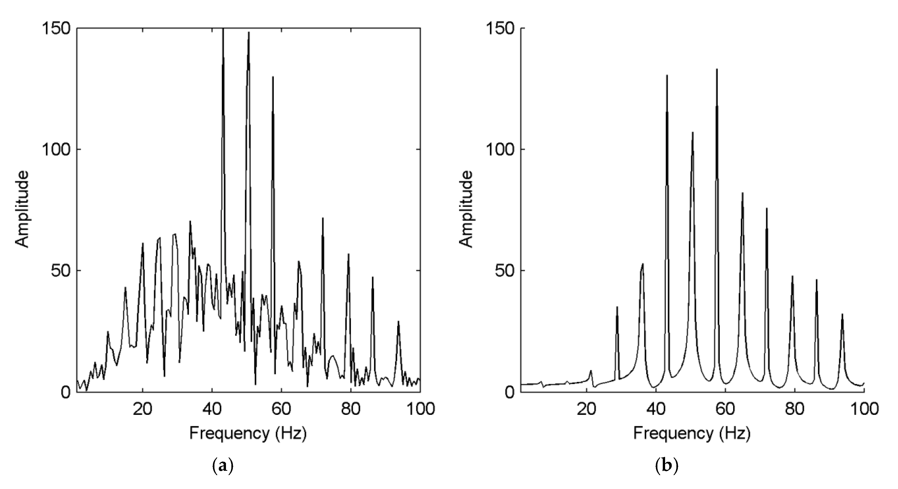
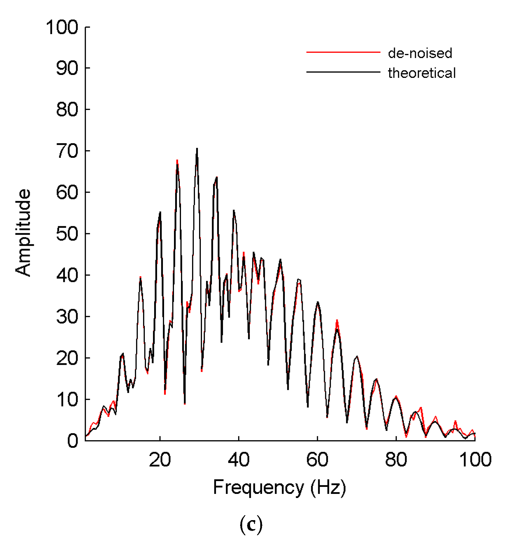
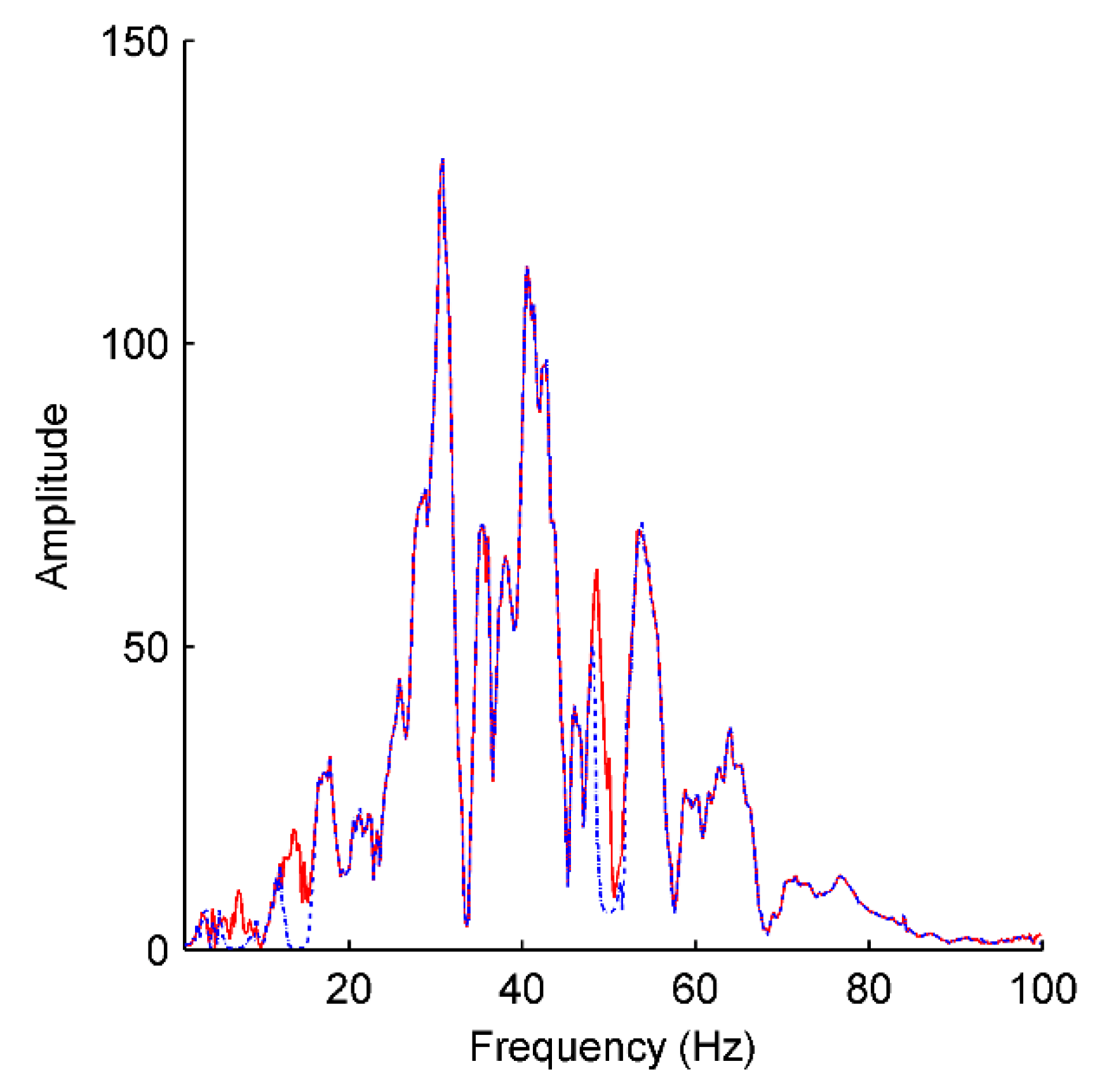
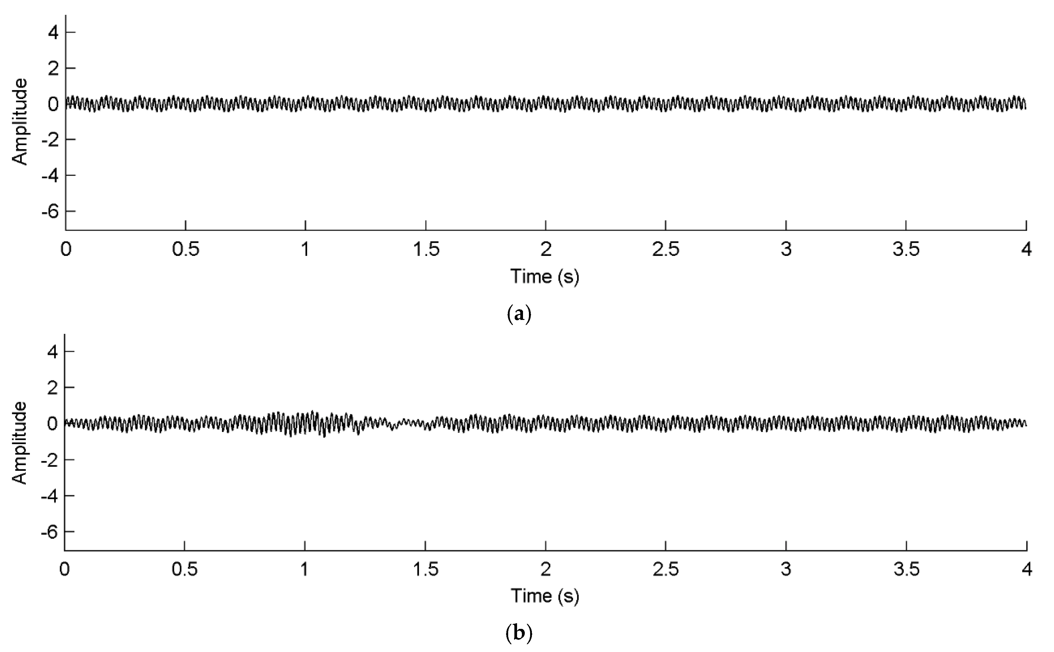
A synthetic signal is shown in Figure 8a, where the main noise is stationary and the waveform is recurring except for weak white Gaussian noise. The eliminated noise and de-noised signal are shown in Figure 8b,c, respectively. Their amplitude spectra are shown in Figure 9. Both the time sequence and amplitude spectrum of the de-noised signal are consistent with the theoretical signal. Because the amplitude spectrum is complex, it is hard to estimate its amplitudes, frequencies and phases, which are important for model-based approaches [8,9]. Therefore, the proposed method can effectively attenuate the multitoned noise and even periodic noise with a complex waveform but not influence the seismic events.
4. Field Example
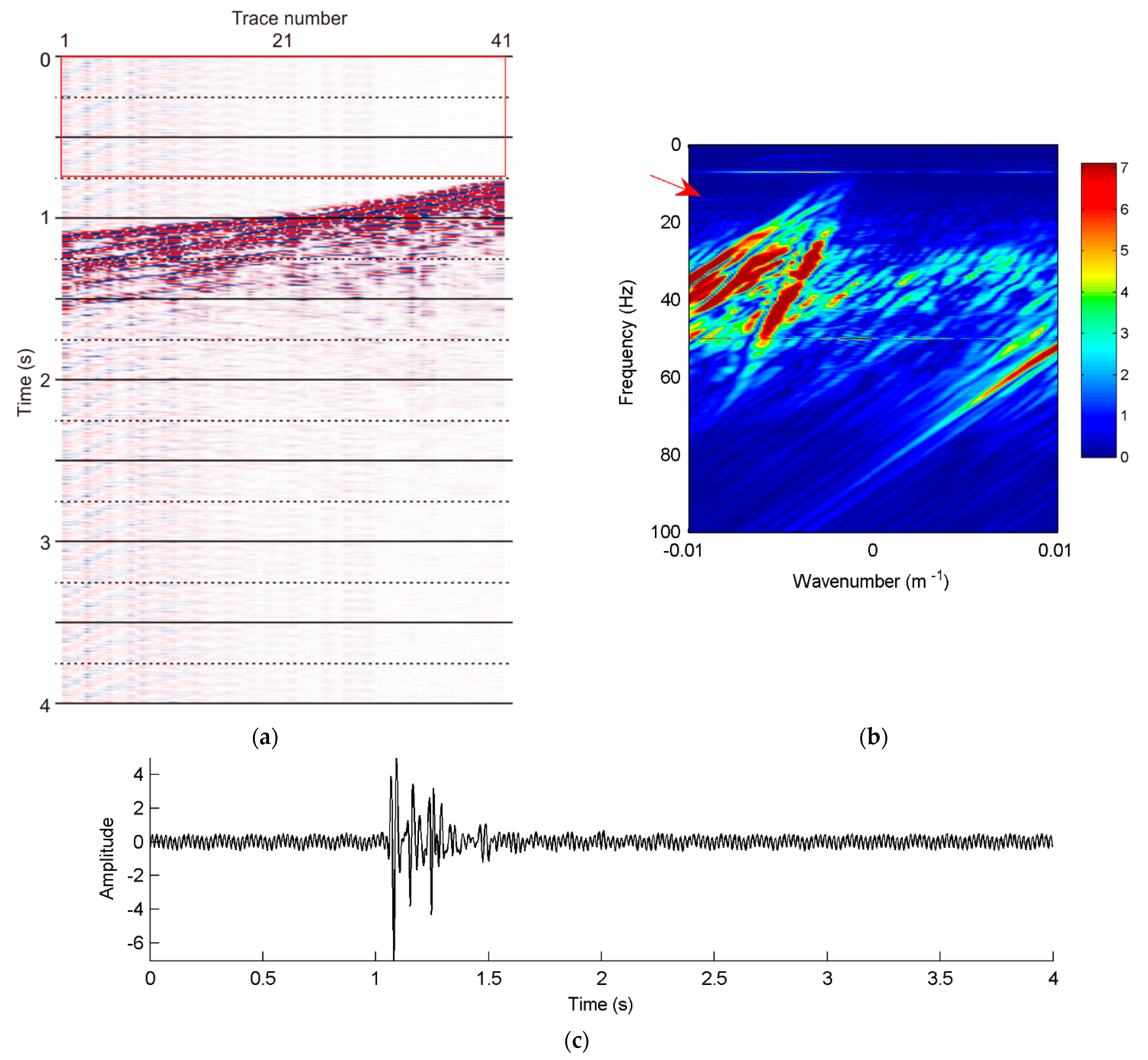
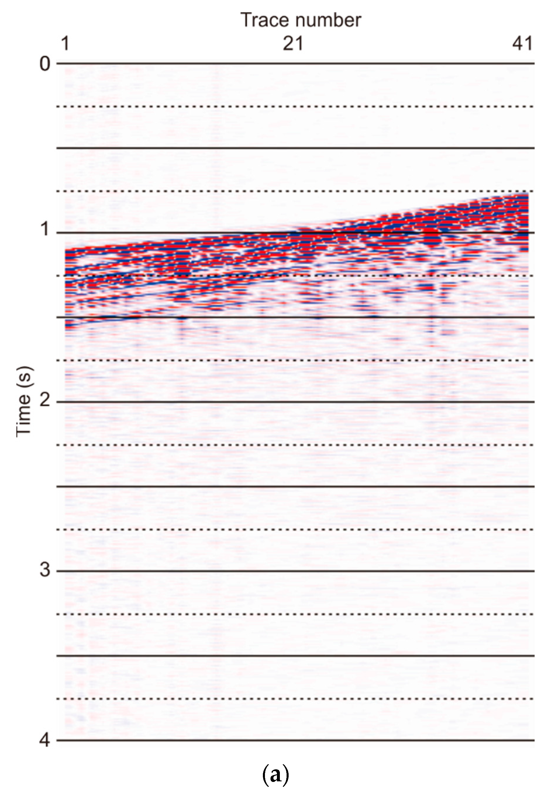
The proposed method was tested using field data. The field data are a land seismic shot recorded with a 2 ms sample rate and a 40 m geophone interval, as shown in Figure 10a. The data contain periodic noise which may be caused by power lines, engine operation and other interferences. The noise is so strong that it affects the quality of the subsequent processes, especially for the first 12 traces. As shown in Figure 10c, we cannot see any waves after the time 1.5 s. There are three horizontal bands around the frequencies of 7 Hz, 14 Hz and 50 Hz in the f-k domain (Figure 10b). The periodic noise at the frequency of approximately 14 Hz, highlighted in Figure 10b, is the weakest, and the periodic noise at the frequency of 50 Hz is the strongest.
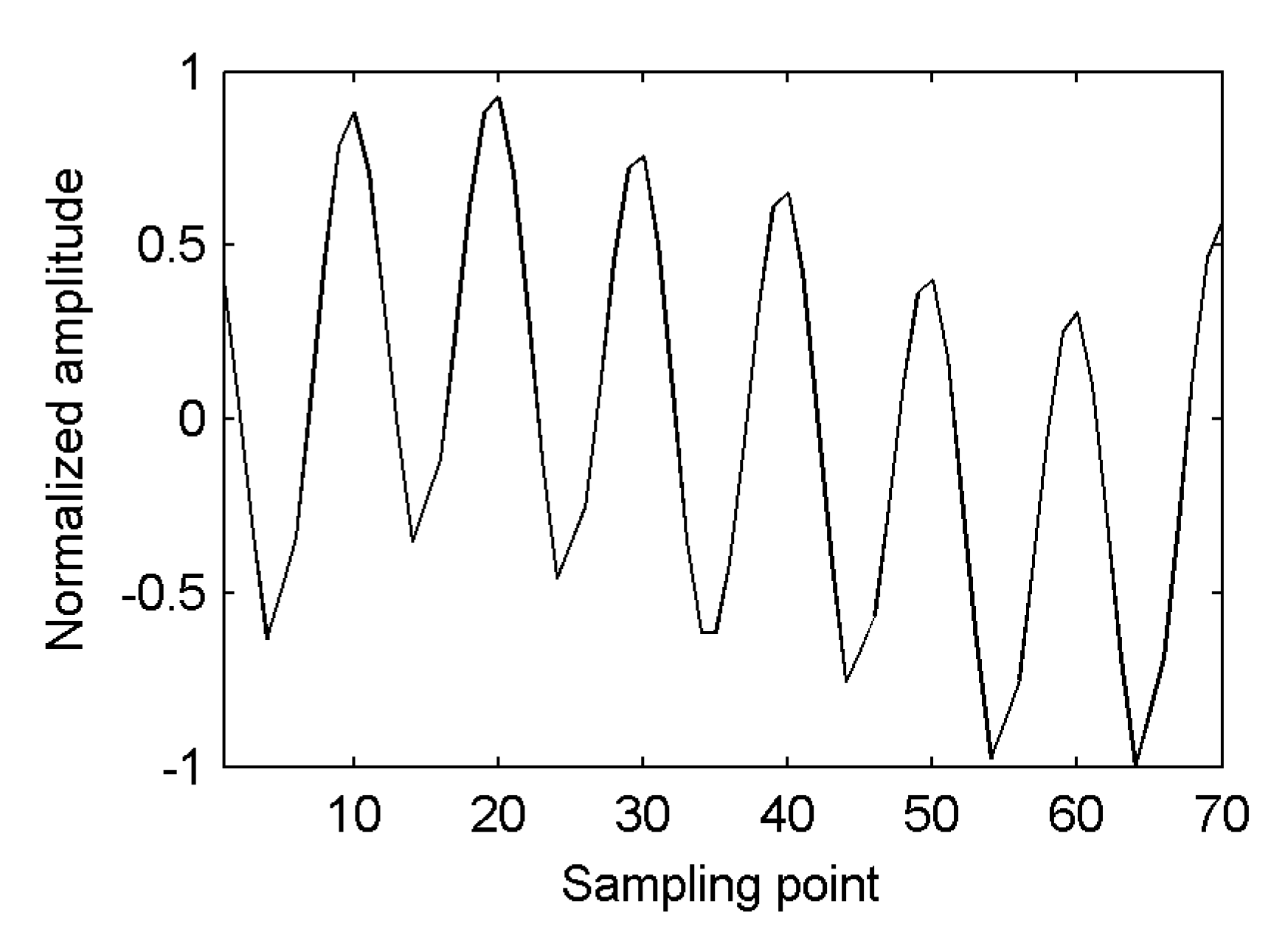
We use the ambient noise marked by a red rectangle in Figure 10a to construct the noise dictionary. The estimated waveform is shown in Figure 11. The result of noise attenuation by the proposed method is shown in Figure 12. The periodic noise is attenuated to a large degree. The horizontal bands of the f-k spectrum are almost eliminated, except for weak residual noise of about 7 Hz frequency. In addition, there are no spectral notches in the f-k spectrum (Figure 12b).
The notch filtering method is applied to the field data for a comparison. The narrow stop band of the notch filter is the frequency range , where is the noise frequency and is the noise bandwidth. The values of for the three noise bands are set to 7 Hz, 14 Hz and 50 Hz, respectively. The noise bandwidth is estimated to be 2 Hz and is set. The f-k spectra of the filtering result are shown in Figure 13. The horizontal bands around the frequencies of 7 Hz, 14 Hz and 50 Hz are separated from the seismic data. However, the seismic waves are also eliminated at those frequencies. This causes spectral notches of seismic waves (Figure 13a). To further show the effectiveness of our method, the spectra of the single-trace de-noised signals by the two methods are compared in Figure 14. For the notch filtering method, the spectral notch causes amplitude loss of seismic events around the frequencies of 7 Hz, 14 Hz and 50 Hz. However, amplitude loss does not occur using our proposed method. The eliminated noise (Figure 15a) is stationary. This is consistent with the characteristics of periodic noise caused by the power lines or engine operation. For comparison, the noise eliminated by the notch filtering method is not stationary because it contains seismic signals.
5. Discussions
The proposed de-noising method is based on sparse representation of periodic noise. The key to our method is the construction of the noise dictionary. Because ambient noise contains no seismic waves but dominant periodic noise and other random noise, periodic noise can be estimated without the influence of seismic reflections. Therefore, our method is useful regardless of whether the seismic waves are strong or weak. A scanning method is used to estimate the noise period. The accuracy of the noise period largely influences our de-noising result. To obtain an accurate noise waveform, the waveforms in the time domain and the space domain are stacked shown as the Equations (5) and (6), respectively. It must be emphasized that our de-noising method is only applicable to stationary noise with a constant period, waveform and amplitude. It can be used to attenuate power line harmonic noise, pump jack noise and engine operation noise in land or oceanic seismic exploration.
Based on the proposed method, ambient noise detection is urged for noise estimation. However, ambient noise has not specifically been detected in oil exploration. Therefore, we suggest that ambient noise should be acquired for one second before source excitation. Long-term ambient noise will be helpful for building a perfect noise dictionary.
Wind- or water-induced noise is not strictly stationary, and the stationarity becomes weak with increasing recording time [22,23]. Our method cannot be used to attenuate this kind of noise. To broaden the method for non-stationary noise, higher-order statistics [24] need to be considered further. In addition, methods of noise feature extraction from ambient noise based on machine learning [25] will draw increased attention in the future.
6. Conclusions
A new method is proposed to attenuate periodic noise based on sparse representation. The novelty is the construction of a noise dictionary based on ambient noise. Our method can attenuate monochromatic or multitoned periodic noise automatically without pre-known noise frequencies. The noise is assumed to be stationary noise with a constant period, waveform and amplitude. Synthetic and field tests show the effectiveness of the proposed method. Compared with the conventional notch filtering method, the proposed method can obtain de-noised data with no distortion in the time and frequency domains. Therefore, our method can attenuate periodic noise without damaging the seismic events.
Author Contributions
Conceptualization, Y.W.; investigation, C.W.; writing—original draft preparation, L.S.; writing—review and editing, L.S. and X.Q.; visualization, X.Q. All authors have read and agreed to the published version of the manuscript.
Funding
This work was supported by the National Natural Science Foundation of China (62127815) and Guizhou Science and Technology Cooperation Platform Talents Program: [2021] 5629.
Institutional Review Board Statement
Not applicable.
Informed Consent Statement
Not applicable.
Data Availability Statement
Not applicable.
Acknowledgments
We thank Yijun Yuan for providing the field data.
Conflicts of Interest
The authors declare no conflict of interest.
References
- Li, G.; Li, Y.; Yang, B. Seismic exploration random noise on land: Modeling and application to noise suppression. IEEE Trans. Geosci. Remote Sens. 2017, 55, 4668–4681. [Google Scholar] [CrossRef]
- Zhong, T.; Zhang, S.; Li, Y.; Yang, B. Simulation of seismic-prospecting random noise in the desert by a brownian-motion-based parametric modeling algorithm. Comptes Rendus Geosci. 2019, 351, 10–16. [Google Scholar] [CrossRef]
- Groos, J.; Ritter, J. Time domain classification and quantification of seismic noise in an urban environment. Geophys. J. Int. 2009, 179, 1213–1231. [Google Scholar] [CrossRef] [Green Version]
- Xu, J.; Wang, W.; Gao, J.; Chen, W. Monochromatic noise removal via sparsity-enabled signal decomposition method. IEEE Geosci. Remote Sens. Lett. 2013, 10, 533–537. [Google Scholar] [CrossRef]
- Meunier, J.; Bianchi, T. Harmonic noise reduction opens the way for array size reduction in vibroseis™ operations. In Seg Tech. Program Expand. Abstr. 2002, 21, 70–73. [Google Scholar] [CrossRef]
- Karsli, H.; Dondurur, D.; Güney, R. A comparison of post-stack results after filtering of harmonic noise using two filter methods. In Proceedings of the Near Surface Geoscience 2016-Second Applied Shallow Marine Geophysics Conference, Barcelona, Spain, 4–8 September 2016. [Google Scholar]
- Larsen, J.J.; Dalgaard, E.; Auken, E. Noise cancelling of mrs signals combining model-based removal of powerline harmonics and multichannel wiener filtering. Geophys. J. Int. 2013, 196, 828–836. [Google Scholar] [CrossRef] [Green Version]
- Yao, J.; Di, D.; Jiang, G.; Gao, S.; Yan, H. Real-time acceleration harmonics estimation for an electro-hydraulic servo shaking table using kalman filter with a linear model. IEEE Trans. Control Syst. Technol. 2014, 22, 794–800. [Google Scholar] [CrossRef]
- Olsson, P.-I.; Fiandaca, G.; Larsen, J.J.; Dahlin, T.; Auken, E. Doubling the spectrum of time-domain induced polarization by harmonic de-noising, drift correction, spike removal, tapered gating and data uncertainty estimation. Geophys. Suppl. Mon. Not. R. Astron. Soc. 2016, 207, 774–784. [Google Scholar] [CrossRef] [Green Version]
- Ghanati, R.; Hafizi, M. Statistical de-spiking and harmonic interference cancellation from surface-nmr signals via a state-conditioned filter and modified nyman-gaiser method. Boll. Di Geofis. Teor. Ed Appl. 2017, 58, 181–204. [Google Scholar]
- Saucier, A.; Marchant, M.; Chouteau, M. A fast and accurate frequency estimation method for canceling harmonic noise in geophysical records. Geophysics 2006, 71, V7–V18. [Google Scholar] [CrossRef]
- Henley, D.C. Spectral clipping: A promax module for attenuating strong monochromatic noise. CREWES Calg. AB Can. 2001, 13, 311–320. [Google Scholar]
- Karslı, H.; Dondurur, D. A mean-based filter to remove power line harmonic noise from seismic reflection data. J. Appl. Geophys. 2018, 153, 90–99. [Google Scholar] [CrossRef]
- Shao, J.; Wang, Y.; Yao, Y.; Wu, S.; Xue, Q.; Chang, X. Simultaneous denoising of multicomponent microseismic data by joint sparse representation with dictionary learning. Geophysics 2019, 84, KS155–KS172. [Google Scholar] [CrossRef]
- Huang, C.C.; Liang, S.F.; Young, M.S.; Shaw, F.Z. A novel application of the s-transform in removing powerline interference from biomedical signals. Physiol. Meas. 2008, 30, 13–27. [Google Scholar] [CrossRef]
- Ghanati, R.; Fallahsafari, M.; Hafizi, M.K. Joint application of a statistical optimization process and empirical mode decomposition to magnetic resonance sounding noise cancelation. J. Appl. Geophys. 2014, 111, 110–120. [Google Scholar] [CrossRef]
- Ghanati, R.; Hafizi, M.K.; Mahmoudvand, R.; Fallahsafari, M. Filtering and parameter estimation of surface-nmr data using singular spectrum analysis. J. Appl. Geophys. 2016, 130, 118–130. [Google Scholar] [CrossRef]
- Wang, D.; Li, Y.; Nie, P. A study on the gaussianity and stationarity of the random noise in the seismic exploration. J. Appl. Geophys. 2014, 109, 210–217. [Google Scholar] [CrossRef]
- Yilmaz, O. Seismic Data Analysis: Processing, Inversion, and Interpretation of Seismic Data; Society of Exploration Geophysicists: Tulsa, OK, USA, 2001. [Google Scholar]
- Mallat, S. A Wavelet Tour of Signal Processing: The Sparse Way, 3rd ed.; Elsevier: Amsterdam, The Netherlands, 2008. [Google Scholar]
- Mallat, S.G.; Zhang, Z. Matching pursuits with time-frequency dictionaries. IEEE Trans. Signal Process. 1993, 41, 3397–3415. [Google Scholar] [CrossRef] [Green Version]
- Zhong, T.; Li, Y.; Wu, N.; Nie, P.; Yang, B. Statistical properties of the random noise in seismic data. J. Appl. Geophys. 2015, 118, 84–91. [Google Scholar] [CrossRef]
- Zhong, T.; Li, Y.; Wu, N.; Nie, P.; Yang, B. A study on the stationarity and gaussianity of the background noise in land-seismic prospecting. Geophysics 2015, 80, V67–V82. [Google Scholar] [CrossRef]
- Mousavi, S.M.; Langston, C.A. Hybrid seismic denoising using higher-order statistics and improved wavelet block thresholding. Bull. Seismol. Soc. Am. 2016, 106, 1380–1393. [Google Scholar] [CrossRef]
- Jia, Y.; Ma, J. What can machine learning do for seismic data processing? An interpolation application. Geophysics 2017, 82, V163–V177. [Google Scholar] [CrossRef]
Figure 1.
Flow skeleton of the proposed method.

Figure 2.
Synthetic seismic data.

Figure 3.
Synthetic contaminated seismic data. (a) Contaminated seismic data in offset-time domain and (b) its frequency-wavenumber (f-k) spectrum where the red rectangle marks the ambient noise we used.
Figure 3.
Synthetic contaminated seismic data. (a) Contaminated seismic data in offset-time domain and (b) its frequency-wavenumber (f-k) spectrum where the red rectangle marks the ambient noise we used.

Figure 4.
Seismic signal on 11th trace. (a) Signal on the 11th trace in time domain and (b) its amplitude spectrum.
Figure 4.
Seismic signal on 11th trace. (a) Signal on the 11th trace in time domain and (b) its amplitude spectrum.

Figure 5.
Noise waveform estimated by the proposed method.

Figure 6.
De-noising result of the synthetic seismic data by the proposed method. (a) De-noised data and (b) eliminated noise by the proposed method; and (c,d) their corresponding f-k spectra.
Figure 6.
De-noising result of the synthetic seismic data by the proposed method. (a) De-noised data and (b) eliminated noise by the proposed method; and (c,d) their corresponding f-k spectra.

Figure 7.
De-noising result on the 11th trace. (a) De-noised signal and (b) eliminated noise on the 11th trace; and (c,d) their amplitude spectra. The red line corresponds to the de-noised signal and the black line corresponds to the theoretical signal in (a,c).
Figure 7.
De-noising result on the 11th trace. (a) De-noised signal and (b) eliminated noise on the 11th trace; and (c,d) their amplitude spectra. The red line corresponds to the de-noised signal and the black line corresponds to the theoretical signal in (a,c).

Figure 8.
De-noising result of the synthetic noisy signal. (a) Noisy signal, (b) eliminated noise and (c) de-noised signal. The de-noised signal is shown as a red line and the theoretical signal as a black line in (c).
Figure 8.
De-noising result of the synthetic noisy signal. (a) Noisy signal, (b) eliminated noise and (c) de-noised signal. The de-noised signal is shown as a red line and the theoretical signal as a black line in (c).

Figure 9.
Amplitude spectra of the (a) noisy signal, (b) eliminated noise and (c) de-noised signal. The de-noised signal is shown as a red line and the theoretical signal as a black line in (c).
Figure 9.
Amplitude spectra of the (a) noisy signal, (b) eliminated noise and (c) de-noised signal. The de-noised signal is shown as a red line and the theoretical signal as a black line in (c).


Figure 10.
Field data. (a) Field data in offset-time domain, (b) its f-k spectrum and (c) the signal on the 8th trace, where the red rectangle marks the ambient noise and the red arrow points to the 14 Hz weak noise.
Figure 10.
Field data. (a) Field data in offset-time domain, (b) its f-k spectrum and (c) the signal on the 8th trace, where the red rectangle marks the ambient noise and the red arrow points to the 14 Hz weak noise.

Figure 11.
Waveform estimated from the ambient noise.

Figure 12.
Result of noise attenuation by our method: (a) de-noised data, (b) its f-k spectrum and (c) the f-k spectrum of eliminated noise.
Figure 12.
Result of noise attenuation by our method: (a) de-noised data, (b) its f-k spectrum and (c) the f-k spectrum of eliminated noise.


Figure 13.
Spectra of (a) the de-noising data and (b) the eliminated noise by the notch filtering method.
Figure 13.
Spectra of (a) the de-noising data and (b) the eliminated noise by the notch filtering method.

Figure 14.
Amplitude spectra of the de-noised signals on the 8th trace by the proposed method (the red solid line) and the notch filtering method (the blue dash-dotted line).
Figure 14.
Amplitude spectra of the de-noised signals on the 8th trace by the proposed method (the red solid line) and the notch filtering method (the blue dash-dotted line).

Figure 15.
Eliminated noise by (a) the proposed method and (b) the notch filtering method.

Disclaimer/Publisher’s Note: The statements, opinions and data contained in all publications are solely those of the individual author(s) and contributor(s) and not of MDPI and/or the editor(s). MDPI and/or the editor(s) disclaim responsibility for any injury to people or property resulting from any ideas, methods, instructions or products referred to in the content. |
© 2023 by the authors. Licensee MDPI, Basel, Switzerland. This article is an open access article distributed under the terms and conditions of the Creative Commons Attribution (CC BY) license (https://creativecommons.org/licenses/by/4.0/).
Share and Cite
MDPI and ACS Style
Sun, L.; Qiu, X.; Wang, Y.; Wang, C. Seismic Periodic Noise Attenuation Based on Sparse Representation Using a Noise Dictionary. Appl. Sci. 2023, 13, 2835. https://0-doi-org.brum.beds.ac.uk/10.3390/app13052835
AMA Style
Sun L, Qiu X, Wang Y, Wang C. Seismic Periodic Noise Attenuation Based on Sparse Representation Using a Noise Dictionary. Applied Sciences. 2023; 13(5):2835. https://0-doi-org.brum.beds.ac.uk/10.3390/app13052835
Chicago/Turabian StyleSun, Lixia, Xinming Qiu, Yun Wang, and Chao Wang. 2023. "Seismic Periodic Noise Attenuation Based on Sparse Representation Using a Noise Dictionary" Applied Sciences 13, no. 5: 2835. https://0-doi-org.brum.beds.ac.uk/10.3390/app13052835
Note that from the first issue of 2016, this journal uses article numbers instead of page numbers. See further details here.