Selection of Additive Manufacturing Machines via Ontology-Supported Multi-Attribute Three-Way Decisions

Abstract

Selection of a suitable additive manufacturing (AM) machine to manufacture a specific product is one of the important tasks in design for AM. So far, many selection approaches based on multi-attribute decision making have been proposed within academia. Each of these approaches works well in its specific context. However, the approaches are not flexible enough and could produce undesirable results as they are all based on multi-attribute two-way decisions. In this paper, a selection approach based on ontology-supported multi-attribute three-way decisions is presented. Firstly, an ontology for AM machine selection is constructed according to vendor documents, benchmark data, expert experience, and the Senvol database. Supported by this ontology, a selection approach based on multi-attribute three-way decisions is then developed. After that, four AM machine selection examples are introduced to illustrate the application of the developed approach. Finally, the effectiveness and advantages of the approach are demonstrated via a set of comparison experiments. The demonstration results suggest that the presented approach is as effective as the existing approaches and more flexible than them when the information for decision making is insufficient or the cost for undesirable decision results is high.

1. Introduction

Additive manufacturing (AM) is a set of emerging manufacturing technologies that provide better design flexibility and geometric complexity, shorter development time, lower manufacturing cost, and less by-product wastes than traditional manufacturing technologies [1,2,3]. Existing AM technologies can be divided into seven categories, which are vat photopolymerization, material jetting, binder jetting, powder bed fusion, material extrusion, directed energy deposition, and sheet lamination [4]. Based on these technologies, more than 3500 types of AM machines have been manufactured and sold in the market [5]. A controversy regarding how one machine is better than the other is meaningless, since each machine has its specific target applications. However, a study on selection of a suitable machine to manufacture a specific product is of necessity and importance [6]. There are two main reasons. First, when selecting an AM machine, multiple factors should be considered comprehensively, such as the configuration, function, performance, utilities, strengths, and limitations of alternative machines and the connections between product requirements [7]. However, an AM machine user usually lacks such experience and basic knowledge. Second, different AM machines may have considerable overlap in many aspects, which would increase the difficulty of AM machine selection in practice [6].

To date, many approaches based on multi-attribute decision making (MADM) [8,9,10,11,12,13,14,15,16,17,18,19,20,21,22,23,24,25,26,27,28,29,30,31,32,33,34,35,36,37,38,39,40,41,42,43,44,45,46,47,48,49,50,51,52,53,54,55,56,57,58,59], as listed in

Table 1. An overview of the forty-eight MADM-based approaches in the literature.

MADM-Based Approach	Specific Techniques	Data Source	Decision-Making Method
Braglia and Petroni (1999) [8]	AHP	EE	Two-way decision
Xu et al. (2001) [9]	KVM	BD	Two-way decision
Byun and Lee (2005) [10]	TOPSIS	BD	Two-way decision
Mahesh et al. (2005) [11]	FS theory	BD	Two-way decision
Wilson and Rosen (2005) [12]	Interval analysis	VD, EE	Two-way decision
Lan et al. (2005) [13]	FSE	——	Two-way decision
Rao and Padmanabhan (2007) [14]	Matrix approach	BD	Two-way decision
Armillotta (2008) [15]	AHP	VD, BD, EE	Two-way decision
Borille et al. (2010) [16]	AHP, MAHP, SPA	BD	Two-way decision
Lokesh and Jain (2010) [17]	AHP	EE	Two-way decision
Rao and Patel (2010) [18]	PROMETHEE	BD	Two-way decision
Zhou and Chen (2010) [19]	AHP	EE	Two-way decision
Chakraborty (2011) [20]	Ratio analysis	BD	Two-way decision
Khrais et al. (2011) [21]	FS theory	EE	Two-way decision
Vahdani et al. (2011) [22]	TOPSIS	BD, EE	Two-way decision
Ic (2012) [23]	TOPSIS	BD	Two-way decision
Mahapatra and Panda (2013) [24]	GRA	EE	Two-way decision
Roberson et al. (2013) [25]	Ranking model	BD	Two-way decision
Liao et al. (2014) [26]	VIKOR	EE	Two-way decision
Vinodh et al. (2014) [27]	VIKOR	EE	Two-way decision
Zhang and Bernard (2014) [28]	DSM	BD	Two-way decision
Zhang et al. (2014) [29]	KVM	BD	Two-way decision
Mancanares et al. (2015) [30]	AHP	VD, EE	Two-way decision
Paul et al. (2015) [31]	Hybrid	——	Two-way decision
Makhesana et al. (2015) [32]	COPRAS	——	Two-way decision
Kek (2016) [33]	FS theory	BD, EE	Two-way decision
Kumar et al. (2016) [34]	ANP	——	Two-way decision
Zheng et al. (2017) [35]	Rough set theory	BD	Two-way decision
Cetinkaya et al. (2017) [36]	Hybrid	——	Two-way decision
Gitinavard et al. (2017) [37]	COPRAS	——	Two-way decision
Anand and Vinodh (2018) [38]	AHP-TOPSIS	EE	Two-way decision
uz Zaman et al. (2018) [39]	AHP	VD	Two-way decision
Wang et al. (2018) [40]	AHP-TOPSIS	BD	Two-way decision
Yildiz et al. (2018) [41]	TOPSIS	——	Two-way decision
Kadkhoda-Ahmadi et al. (2019) [42]	AHP	VD, BD, EE	Two-way decision
Moiduddin et al. (2019) [43]	Hybrid	——	Two-way decision
Prabhu et al. (2019) [44,45]	Hybrid	——	Two-way decision
Raigar et al. (2020) [46]	Hybrid	——	Two-way decision
Qin et al. (2020) [47,48,49]	AOs	——	Two-way decision
Liu et al. (2020) [50]	AHP	——	Two-way decision
Prabhu et al. (2020) [51]	PSI	——	Two-way decision
Bikas et al. (2021) [52]	AHP	——	Two-way decision
Saxena et al. (2021) [53]	TOPSIS	——	Two-way decision
Ransikarbum et al. (2021) [54]	Hybrid	——	Two-way decision
Psarommatis et al. (2022) [55]	AHP	——	Two-way decision
Raja et al. (2022) [56]	AHP	——	Two-way decision
Raja et al. (2022) [57]	TOPSIS	——	Two-way decision
Chandra et al. (2022) [58]	Hybrid	——	Two-way decision

Notes: AHP refers to analytic hierarchy process; KVM refers to knowledge value measuring; MAHP refers to multiplicative analytic hierarchy process; SPA refers to simple pair analysis; GRA refers to grey relational analysis; VIKOR refers to vlsekriterijuska optimizacija i komoromisno resenje; DSM refers to deviation-similarity model; PROMETHEE refers to preference ranking organization method for enrichment evaluation; TOPSIS refers to technique for order of preference by similarity to ideal solution; AOs refers to aggregation operators; COPRAS refers to complex proportional assessment; FSE refers to fuzzy synthetic evaluation; PSI refers to preference selection index; ANP refers to analytical network process; EE refers to expert experience; BD refers to benchmark data; and VD refers to vendor documents.

, have been proposed to solve the problem of AM machine selection [6]. Each of these approaches works well in its specific context. However, the approaches are not flexible enough and could produce undesirable results as they are all based on multi-attribute two-way decisions. In multi-attribute two-way decisions, the decision regarding each alternative is either acceptance or rejection, which is simple and direct. However, this would hastily classify the alternatives at the border of acceptance or rejection, so that could generate unreasonable decision results. In addition, the values of attributes of an AM machine are generally collected from users from online databases, vendor documents, benchmark data, and expert experience; this is tedious and error-prone. This necessitates a way to automatically generate the information for decision making on demand.

In this paper, an AM machine selection approach based on ontology-supported multi-attribute three-way decisions is proposed. This approach uses ontologies [60] to model the online database. Benefiting from the automatic reasoning capability of an ontology, the approach can automatically generate the information for AM machine selection on demand. Further, alternative AM machines are rated via multi-attribute three-way decisions in the proposed approach. Compared to multi-attribute two-way decisions, this method provides an additional abstaining decision for an alternative, which avoids premature classification of the alternatives at the state of hesitation. Because of this, the proposed approach is more flexible and advantageous than those based on multi-attribute two-way decisions.

The remaining content of this paper is arranged as follows: Section 2 explains the details of the proposed approach. Section 3 illustrates the application of the approach via four AM machine selection examples. Section 4 demonstrates the effectiveness and advantages of the approach via two comparison experiments. Section 5 provides a detailed summary.

2. The Proposed Approach

In this section, the proposed AM machine selection approach based on ontology-supported multi-attribute three-way decisions is described in detail. The proposed approach first obtains all AM machines, attributes, and attribute values and formalizes them in a description logic (DL) ontology.

Because the DL ontology has the advantage of knowledge reasoning, corresponding attribute values are automatically generated according to the AM machines to be selected and the attributes to be considered. Then, AM machine selection is carried out via multi-attribute three-way decisions.

2.1. DL Ontology for AM Machine Selection

A DL ontology for AM machine selection was created in Protege [61]. The DL ontology takes the alternative AM machines and attributes as inputs and the corresponding attribute values as outputs. Thus, the automatic acquisition of attribute values can be realized. In this paper, six AM processes (EBM, SLM, LENS, DMLS, SLS, DMD) and seven attributes (Capability, Strength, Build Time, Density, Part Cost, Complexity, Hardness) are used to describe the developed DL ontology. Fifteen top-level concepts are depicted in Figure 1. These concepts are all atomic concepts.

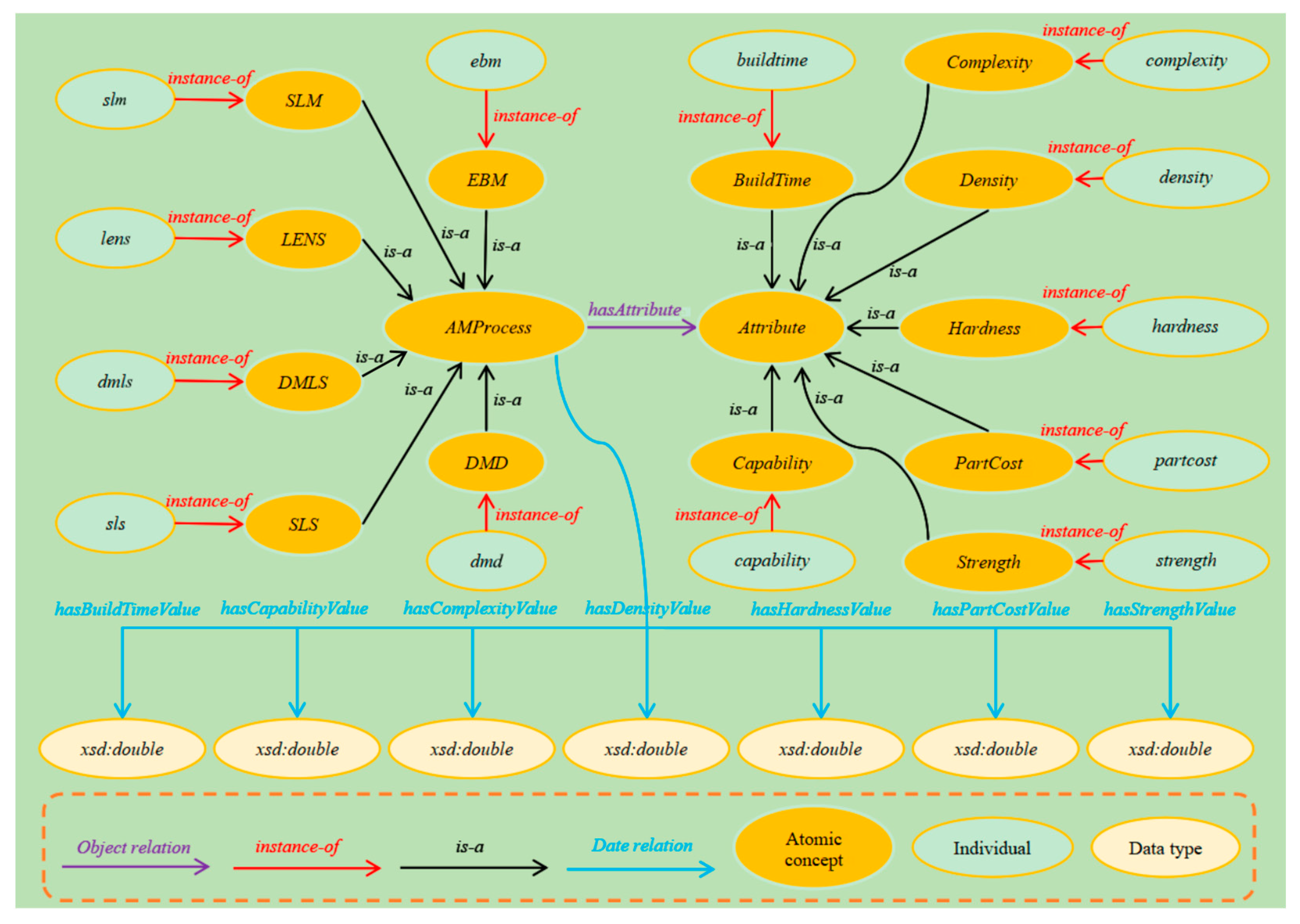
To represent the data and knowledge for automatic generation of AM machine attribute values, an object relation named hasAttribute; seven data relations named hasBuildTimeValue, hasCapabilityValue, hasComplexityValue, hasDensityValue, hasHardnessValue, hasPartCostValue, and hasStrengthValue; and 13 individuals named dmd, dmls, ebm, lens, slm, sls, buildtime, capability, complexity, density, hardness, partcost, and strength are also created in the DL ontology. Based on the created entities, an ontological view of automatic generation of AM machine attribute values is depicted in Figure 2.

2.2. Concepts and Rules for Multi-Attribute Three-Way Decisions

In AM machine selection, each attribute of alternatives needs to be evaluated. Due to different evaluation criteria (e.g., $0~1$, $1~9$, $0~10$, etc.), data processing will become complex, and attribute values may be wrong due to the conversion of the evaluation criteria. Therefore, in order to guarantee the consistency and reliability of evaluation, the evaluation criteria for attribute values in the proposed approach are $0~1$ (i.e., $x_{ij}\in \left[0, 1\right]$). Next, some concepts and rules for explaining the multi-attribute three-way decisions [62] are defined.

2.2.1. Relative Loss Function

The relative loss function is given in

Table 2. Relative loss function.

${\mathit{A}}_{\mathit{i}}$	${\mathit{C}}_{\mathit{j}}\left(\mathit{P}\right)$	$\neg {\mathit{C}}_{\mathit{j}}\left(\mathit{N}\right)$
${\mathit{a}}_{\mathit{p}}$	$0$	${\lambda }_{PN}^{{}^{\prime }}$
${\mathit{a}}_{\mathit{B}}$	${\lambda }_{BP}^{{}^{\prime }}$	${\lambda }_{BN}^{{}^{\prime }}$
${\mathit{a}}_{\mathit{N}}$	${\lambda }_{NP}^{{}^{\prime }}$	$0$

.

${\lambda }_{BP}^{{}^{\prime }}$ represents alternative $A_i$ that has attribute $C_j\left(P\right)$ to make the noncommitment decision $a_B$, and the loss value is ${\lambda }_{BP}^{{}^{\prime }}$;

${\lambda }_{NP}^{{}^{\prime }}$ represents alternative $A_i$ that has attribute $C_j\left(P\right)$ to make the rejection decision $a_N$, and the loss value is ${\lambda }_{NP}^{{}^{\prime }}$;

${\lambda }_{PN}^{{}^{\prime }}$ represents alternative $A_i$ that has no attribute $C_j\left(P\right)$ to make the acceptance decision $a_P$, and the loss value is ${\lambda }_{PN}^{{}^{\prime }}$;

${\lambda }_{BN}^{{}^{\prime }}$ represents alternative $A_i$ that has no attribute $C_j\left(P\right)$ to make the noncommitment decision $a_B$, and the loss value is ${\lambda }_{BN}^{{}^{\prime }}$;

$C_j\left(P\right)$, $\neg C_j\left(N\right)$ indicates two states such that $C_j\left(P\right)\cup \neg C_j\left(N\right)=\Omega$, $A_i$∈$C_j\left(P\right)$, which indicates that $A_i$ has attribute $C_j\left(P\right)$, $A_i\in \neg C_j\left(N\right)$, which indicates that $A_i$ does not have attribute $C_j\left(P\right)$;

$a_P$, $a_B$, and $a_N$, respectively, represent the decisions made: acceptance ($POS\left(C\right)$), noncommitment ($BND\left(C\right)$), and rejection ($NEG\left(C\right)$).

2.2.2. Relative Loss Function of Attribute Values

The relative loss function of attribute values is given in

Table 3. Relative loss function of attribute values.

${\mathit{A}}_{\mathit{i}}$	${\mathit{C}}_{\mathit{j}}\left(\mathit{P}\right)$	$\neg {\mathit{C}}_{\mathit{j}}\left(\mathit{N}\right)$
${\mathit{a}}_{\mathit{p}}$	$0$	$x_{max}^{{}^{″}}-x_{ij}^{{}^{″}}$
${\mathit{a}}_{\mathit{B}}$	${\sigma }_j\left(x_{ij}^{{}^{″}}-x_{min}^{{}^{″}}\right)$	${\sigma }_j\left(x_{max}^{{}^{″}}-x_{ij}^{{}^{″}}\right)$
${\mathit{a}}_{\mathit{N}}$	$x_{ij}^{{}^{″}}-x_{min}^{{}^{″}}$	$0$

.

${\lambda }_{BP}^{{}^{\prime }}={\sigma }_j\left(x_{ij}^{{}^{″}}-x_{min}^{{}^{″}}\right)$ represents alternative $A_i$, which has attributes $C_j\left(P\right)$ to make the noncommitment decision $a_B$, and the loss value is ${\sigma }_j\left(x_{ij}^{{}^{″}}-x_{min}^{{}^{″}}\right)$;

${\lambda }_{NP}^{{}^{\prime }}=x_{ij}^{{}^{″}}-x_{min}^{{}^{″}}$ represents alternative $A_i$, which has attributes $C_j\left(P\right)$ to make the rejection decision $a_N$, and the loss value is $x_{ij}^{{}^{″}}-x_{min}^{{}^{″}}$;

${\lambda }_{PN}^{{}^{\prime }}=x_{max}^{{}^{″}}-x_{ij}^{{}^{″}}$ represents alternative $A_i$, which has no attribute $C_j\left(P\right)$ to make the acceptance decision $a_P$, and the loss value is $x_{max}^{{}^{″}}-x_{ij}^{{}^{″}}$;

${\lambda }_{BN}^{{}^{\prime }}={\sigma }_j\left(x_{max}^{{}^{″}}-x_{ij}^{{}^{″}}\right)$ represents alternative $A_i$, which has no attribute $C_j\left(P\right)$ to make the noncommitment decision $a_B$, and the loss value is ${\sigma }_j\left(x_{max}^{{}^{″}}-x_{ij}^{{}^{″}}\right)$;

$x_{min}^{{}^{″}}$ is in the normalized fuzzy decision matrix $M^{{}^{″}}$, $x_{min}^{{}^{″}}=0$;

$x_{max}^{{}^{″}}$ is in the normalized fuzzy decision matrix $M^{{}^{″}}$, $x_{max}^{{}^{″}}=1$;

${\sigma }_j$ is the risk coefficient of attributes given by a user, ${\sigma }_j\in \left[0, 0.5\right]$, when ${\sigma }_j=0.5$, multi-attribute three-way decisions will reduce to multi-attribute two-way decisions; if the user prefers accurate results, a large value can be assigned; if the user prefers fuzzy results, a small value can be assigned;

$C_j\left(P\right)$, $\neg C_j\left(N\right)$ indicate two states such that $C_j\left(P\right)\cup \neg C_j\left(N\right)=\Omega$; $A_i$∈$C_j\left(P\right)$ indicates that $A_i$ has attribute $C_j\left(P\right)$; and $A_i\in \neg C_j\left(N\right)$ indicates that $A_i$ does not have attribute $C_j\left(P\right)$.

$a_P$, $a_B$, $a_N$, respectively, represent the decisions made: acceptance ($POS\left(C\right)$), noncommitment ($BND\left(C\right)$), and rejection ($NEG\left(C\right)$).

2.2.3. Comprehensive Relative Loss Function of Alternatives

The comprehensive relative loss function of alternatives is given in

Table 4. Comprehensive relative loss function of alternatives.

${\mathit{A}}_{\mathit{i}}$	${\mathit{C}}_{\mathit{j}}\left(\mathit{P}\right)$	$\neg {\mathit{C}}_{\mathit{j}}\left(\mathit{N}\right)$
${\mathit{a}}_{\mathit{p}}$	$0$	$x_{max}^{{}^{″}}-{{\displaystyle \sum }}_{j=1}^n{w}_j{x}_{ij}^{{}^{″}}$
${\mathit{a}}_{\mathit{B}}$	${{\displaystyle \sum }}_{j=1}^n{\sigma }_j{w}_j\left(x_{ij}^{{}^{″}}-x_{min}^{{}^{″}}\right)$	${{\displaystyle \sum }}_{j=1}^n{\sigma }_j{w}_j\left(x_{max}^{{}^{″}}-x_{ij}^{{}^{″}}\right)$
${\mathit{a}}_{\mathit{N}}$	${{\displaystyle \sum }}_{j=1}^n{w}_j{x}_{ij}^{{}^{″}}-x_{min}^{{}^{″}}$	$0$

.

${\lambda }_{BP}^{{}^{\prime }}={\displaystyle \sum }_{j=1}^n{\sigma }_j{w}_j\left(x_{ij}^{{}^{″}}-x_{min}^{{}^{″}}\right)$ represents alternative $A_i$ that has attribute $C_j\left(P\right)$ to make the noncommitment decision $a_B$, and the loss value is ${\displaystyle \sum }_{j=1}^n{\sigma }_j{w}_j\left(x_{ij}^{{}^{″}}-x_{min}^{{}^{″}}\right)$;

${\lambda }_{NP}^{{}^{\prime }}={{\displaystyle \sum }}_{j=1}^n{w}_j{x}_{ij}^{{}^{″}}-x_{min}^{{}^{″}}$ represents alternative $A_i$ that has attribute $C_j\left(P\right)$ to make the rejection decision $a_N$, and the loss value is ${{\displaystyle \sum }}_{j=1}^n{w}_j{x}_{ij}^{{}^{″}}-x_{min}^{{}^{″}}$;

${\lambda }_{PN}^{{}^{\prime }}=x_{max}^{{}^{″}}-{{\displaystyle \sum }}_{j=1}^n{w}_j{x}_{ij}^{{}^{″}}$ represents alternative $A_i$ that has no attribute $C_j\left(P\right)$ to make the acceptance decision $a_P$, and the loss value is $x_{max}^{{}^{″}}-{{\displaystyle \sum }}_{j=1}^n{w}_j{x}_{ij}^{{}^{″}}$;

${\lambda }_{BN}^{{}^{\prime }}={{\displaystyle \sum }}_{j=1}^n{\sigma }_j{w}_j\left(x_{max}^{{}^{″}}-x_{ij}^{{}^{″}}\right)$ represents alternative $A_i$ that has no attribute $C_j\left(P\right)$ to make the noncommitment decision $a_B$, and the loss value is ${{\displaystyle \sum }}_{j=1}^n{\sigma }_j{w}_j\left(x_{max}^{{}^{″}}-x_{ij}^{{}^{″}}\right)$;

$x_{min}^{{}^{″}}$ is in the normalized fuzzy decision matrix $M^{{}^{″}}$, $x_{min}^{{}^{″}}=0$;

$x_{max}^{{}^{″}}$ is inn the normalized fuzzy decision matrix $M^{{}^{″}}$, $x_{max}^{{}^{″}}=1$;

${\sigma }_j$ is the risk coefficient of attributes given by a user, ${\sigma }_j\in \left[0, 0.5\right]$, when ${\sigma }_j=0.5$, multi-attribute three-way decisions will reduce to multi-attribute two-way decisions; if the user prefers accurate results, a large value can be assigned; if the user prefers fuzzy results, a small value can be assigned;

$C_j\left(P\right)$, $\neg C_j\left(N\right)$ indicate two states such that $C_j\left(P\right)\cup \neg C_j\left(N\right)=\Omega$; $A_i$∈$C_j\left(P\right)$ indicates that $A_i$ has attribute $C_j\left(P\right)$; and $A_i\in \neg C_j\left(N\right)$ indicates that $A_i$ does not have attribute $C_j\left(P\right)$;

$a_P$, $a_B$, $a_N$, respectively, represent the decisions made: acceptance ($POS\left(C\right)$), noncommitment ($BND\left(C\right)$), and rejection ($NEG\left(C\right)$);

$w_j$ is weights of attributes for alternative AM machines.

2.2.4. Comprehensive Thresholds of Alternatives

$${\alpha }_i=\frac{{{\displaystyle \sum }}_{j=1}^n{w}_j\left(1-{\sigma }_j\right)\left(x_{max}^{{}^{″}}-x_{ij}^{{}^{″}}\right)}{{{\displaystyle \sum }}_{j=1}^n{w}_j\left(1-{\sigma }_j\right)\left(x_{max}^{{}^{″}}-x_{ij}^{{}^{″}}\right)+{{\displaystyle \sum }}_{j=1}^n{w}_j{\sigma }_j\left(x_{ij}^{{}^{″}}-x_{min}^{{}^{″}}\right)}$$

(1)

$${\beta }_i=\frac{{{\displaystyle \sum }}_{j=1}^n{w}_j{\sigma }_j\left(x_{max}^{{}^{″}}-x_{ij}^{{}^{″}}\right)}{{{\displaystyle \sum }}_{j=1}^n{w}_j{\sigma }_j\left(x_{max}^{{}^{″}}-x_{ij}^{{}^{″}}\right)+{{\displaystyle \sum }}_{j=1}^n{w}_j\left(1-{\sigma }_j\right)\left(x_{ij}^{{}^{″}}-x_{min}^{{}^{″}}\right)}$$

(2)

$x_{min}^{{}^{″}}$ is in the normalized fuzzy decision matrix $M^{{}^{″}}$, $x_{min}^{{}^{″}}=0$;

$x_{max}^{{}^{″}}$ is in the normalized fuzzy decision matrix $M^{{}^{″}}$, $x_{max}^{{}^{″}}=1$;

$w_j$ is weights of attributes for alternative AM machines;

${\sigma }_j$ the risk coefficient of attributes given by a user, ${\sigma }_j\in \left[0, 0.5\right]$, when ${\sigma }_j=0.5$, multi-attribute three-way decisions will reduce to multi-attribute two-way decisions; if the user prefers accurate results, a large value can be assigned; if the user prefers fuzzy results, a small value can be assigned.

2.2.5. Rules for Multi-Attribute Three-Way Decisions

To provide semantic interpretations of the thresholds and three regions in probabilistic rough sets, Yao [63] created decision theoretic rough sets (DTRS) with the use of Bayesian theory.

Table 5. The loss function.

${\mathit{A}}_{\mathit{i}}$	${\mathit{C}}_{\mathit{j}}\left(\mathit{P}\right)$	$\neg {\mathit{C}}_{\mathit{j}}\left(\mathit{N}\right)$
${\mathit{a}}_{\mathit{p}}$	${\lambda }_{PP}$	${\lambda }_{PN}$
${\mathit{a}}_{\mathit{B}}$	${\lambda }_{BP}$	${\lambda }_{BN}$
${\mathit{a}}_{\mathit{N}}$	${\lambda }_{NP}$	${\lambda }_{NN}$

lists the two states and three actions that make up a DTRS model.

For $\forall x\in U$, we denote $R(a_i|\left[x\right])$ as the expected loss when taking the action $a_i\left(i=P, B, N\right)$, and according to Table 5 it can be calculated as [62]:

$$R(a_P|\left[x\right])={\lambda }_{PP}Pr(C|\left[x\right])+{\lambda }_{PN}Pr(\neg C|\left[x\right])$$

(3)

$$R(a_B|\left[x\right])={\lambda }_{BP}Pr(C|\left[x\right])+{\lambda }_{BN}Pr(\neg C|\left[x\right])$$

(4)

$$R(a_N|\left[x\right])={\lambda }_{NP}Pr(C|\left[x\right])+{\lambda }_{NN}Pr(\neg C|\left[x\right])$$

(5)

The conditional probability of an object $x$ belonging to $C$, given that the object is described by its equivalence class $\left[x\right]$, can be expressed as $Pr(C|\left[x\right])$ [64]. Note that $Pr(\neg C|\left[x\right])=1-Pr(C|\left[x\right])$.

According to Bayesian theory, the best decision is the one with minimum loss, so rules for multi-attribute three-way decisions can be indicated as follows:

$$\begin{gathered} \mathrm{If} min(R(a_P|\left[x\right]), R(a_B|\left[x\right]), R(a_N|\left[x\right]))=R(a_P|\left[x\right]), \mathrm{decide} x\in POS\left(C\right) \\ \mathrm{If} min(R(a_P|\left[x\right]), R(a_B|\left[x\right]), R(a_N|\left[x\right]))=R(a_B|\left[x\right]), \mathrm{decide} x\in BND\left(C\right) \\ \mathrm{If} min(R(a_P|\left[x\right]), R(a_B|\left[x\right]), R(a_N|\left[x\right]))=R(a_N|\left[x\right]), \mathrm{decide} x\in NEG\left(C\right) \end{gathered}$$

2.3. Specific Steps of the Proposed Approach

An AM machine selection problem can be described thus: $m$ alternative AM machines $A_1~A_m$, n attributes $c_1~c_n$, and n weights of attributes $w_1~w_n$ such that $w_j$ is the weight of the attribute $c_j$, $w_1~w_n\in \left[0, 1\right]$ and ${\displaystyle \sum }_{j=1}^n{w}_j=1$, and a decision matrix $M={\left[x_{ij}\right]}_{m\times n} (i\in \left[1, m\left]; j\in \right[1, n\right]; x_{ij}>0)$ such that $x_{ij}$ is the values corresponding to attribute $c_j$ of alternative $A_i$. Based on these components, the AM machine selection problem can be solved by evaluating each alternative $A_i$ according to the weight $w_j$ of each attribute and the decision matrix $M$ [62]. The specific process mainly includes the following steps:

• Generate the values of attributes.

According to the alternative AM machines and attributes of an AM machine selection problem, the values of attributes are automatically generated by the automatic reasoning of the developed DL ontology for AM machine selection.

2.

Construct a decision matrix $M$.

According to the attribute values generated by the DL ontology, a decision matrix $M$ is established as:

$$M=\left[\begin{array}{c}\begin{array}{cccc}{x}_{11}& x_{12}& \cdots & x_{1n}\\ x_{21}& x_{22}& \cdots & x_{2n}\\ ⋮& ⋮& \ddots & ⋮\\ x_{m1}& x_{m2}& \dots & x_{mn}\end{array}\end{array}\right]$$

3.

Construct a fuzzy decision matrix $M^{{}^{\prime }}$.

The decision matrix $M$ is fuzzified using:

$$x_{ij}^{{}^{\prime }}=\frac{x_{ij}}{\sqrt{{{\displaystyle \sum }}_{i=1}^m{x}_{ij}^2}}$$

(6)

where $x_{ij}$ indicates the attribute value of the j-th attribute of the i-th alternative.

Then a fuzzy decision matrix $M^{{}^{\prime }}$ is obtained as:

$$M^{{}^{\prime }}=\left[\begin{array}{c}\begin{array}{cccc}\langle x_{11}^{{}^{\prime }}\rangle & \langle x_{12}^{{}^{\prime }}\rangle & \cdots & \langle x_{1n}^{{}^{\prime }}\rangle \\ \langle x_{21}^{{}^{\prime }}\rangle & \langle x_{22}^{{}^{\prime }}\rangle & \cdots & \langle x_{2n}^{{}^{\prime }}\rangle \\ ⋮& ⋮& \ddots & ⋮\\ \langle x_{m1}^{{}^{\prime }}\rangle & \langle x_{m2}^{{}^{\prime }}\rangle & \dots & \langle x_{mn}^{{}^{\prime }}\rangle \end{array}\end{array}\right]$$

4.

Construct a normalized fuzzy decision matrix $M^{{}^{″}}$.

In an AM machine selection problem, there are two types of attributes (i.e., positive attributes and negative attributes), in which a positive attribute has a positive impact on decision making, and a negative attribute has a negative impact on decision making. In order to eliminate such influences, a complement rule is needed to transform negative attributes into positive attributes [65]:

$$x_{ij}^{{}^{″}}=\left\{\begin{array}{cc}{x}_{ij}^{{}^{\prime }}& if c_j is a positive criterion\\ 1-x_{ij}^{{}^{\prime }}& if c_j is a negative criterion\end{array}\right.$$

(7)

Thus, a fuzzy decision matrix $M^{{}^{\prime }}$ is transformed into a normalized fuzzy decision matrix $M^{{}^{″}}$.

$$M^{{}^{″}}=\left[\begin{array}{c}\begin{array}{cccc}\langle x_{11}^{{}^{″}}\rangle & \langle x_{12}^{{}^{″}}\rangle & \cdots & \langle x_{1n}^{{}^{″}}\rangle \\ \langle x_{21}^{{}^{″}}\rangle & \langle x_{22}^{{}^{″}}\rangle & \cdots & \langle x_{2n}^{{}^{″}}\rangle \\ ⋮& ⋮& \ddots & ⋮\\ \langle x_{m1}^{{}^{″}}\rangle & \langle x_{m2}^{{}^{″}}\rangle & \dots & \langle x_{mn}^{{}^{″}}\rangle \end{array}\end{array}\right]$$

5.

Calculate the relative loss function of the attributes considered for each alternative.

The calculation method is shown in Table 3.

6.

Calculate the comprehensive relative loss function of each alternative.

The calculation method is shown in Table 4.

7.

Calculate the comprehensive thresholds ${\alpha }_i$ and ${\beta }_i$ of each alternative.

According to Equations (1) and (2), the comprehensive thresholds ${\alpha }_i$ and ${\beta }_i$ of the alternatives are calculated.

8.

Make the judgment of each alternative.

$$Pr(C|\left[A_i\right])\ge {\alpha }_i\hspace{1em}\hspace{1em}\hspace{1em}\hspace{1em}\mathrm{Decide}: A_i\in POS\left(C\right);$$

(8)

$${\beta }_i<\mathit{Pr}\left(C|\left[A_i\right]\right)<{\alpha }_i\hspace{1em}\hspace{1em}\hspace{1em}\hspace{1em}\mathrm{Decide}: A_i\in BND\left(C\right);$$

(9)

$$Pr(C|\left[A_i\right])\le {\beta }_i\hspace{1em}\hspace{1em}\hspace{1em}\hspace{1em}\mathrm{Decide}: A_i\in NEG\left(C\right).$$

(10)

$Pr\left(\left.C\right|\left[A_i\right]\right)$ represents the conditional probability of the alternative AM machine $A_i$. $Pr\left(\left.C\right|\left[A_i\right]\right)$ can be calculated using the method in [66,67,68]. By comparing the conditional probability $Pr\left(\left.C\right|\left[A_i\right]\right)$ with the comprehensive thresholds ${\alpha }_i$ and ${\beta }_i$ of the alternative $A_i$, the judgment of the alternative $A_i$ is made: acceptance ($POS\left(C\right)$), noncommitment ($BND\left(C\right)$), or rejection($NEG\left(C\right)$).

3. Application

In this section, four AM machine selection examples are introduced to illustrate the application of the proposed approach.

Example 1 [12]: DMD (Direct Metal Deposition), DMLS (Direct Metal Laser Sintering), EBM (Electron Beam Melting), LENS (Laser Engineered Net Shaping), SLM (Selective Laser Melting), and SLS (Selective Laser Sintering) are six AM processes. One AM machine is selected under each AM process, which makes up six alternative AM machines. This article still uses each AM process to represent its corresponding AM machine. The attributes used to select these AM machines are ultimate tensile strength (MPa), Rockwell hardness (HRC), density (%), detail capability (mm), geometric complexity (nmu), build time (hrs), and part cost ($).

Table 6. Example 1 $\sigma =\left(0.35, 0.4, 0.4, 0.4, 0.5, 0.35, 0.4\right)$.

AM Machine	$\left({\mathit{c}}_1\right)$ Strength	$\left({\mathit{c}}_2\right)$ Hardness	$\left({\mathit{c}}_3\right)$ Density	$\left({\mathit{c}}_4\right)$ Capability	$\left({\mathit{c}}_5\right)$ Complexity	$\left({\mathit{c}}_6\right)$ Build Time	$\left({\mathit{c}}_7\right)$ Part Cost
$\left(A_1\right)$ DMD	1800	53	100	1.016	6	25.44	77.78
$\left(A_2\right)$ DMLS	600	21	95	0.300	10	41.47	1150.18
$\left(A_3\right)$ EBM	1430	50	100	1.200	10	10.41	315.03
$\left(A_4\right)$ LENS	1703	53	100	0.762	6	5.03	145.51
$\left(A_5\right)$ SLM	2000	60	99.5	0.150	10	27.45	679.15
$\left(A_6\right)$ SLS	606	15	100	0.600	10	41.47	453.27

lists the alternative AM machines and the attributes considered for each alternative. The weights of the seven attributes are 0.167, 0.144, 0.071, 0.024, 0.214, 0.190, and 0.190.

Example 2 [10]: SLA3500, SLS2500, FDM8000, LOM1015, Quadra, and Z402 are six alternative AM machines. The attributes used to select these AM machines are dimensional accuracy ($\mathsf{\mu }\mathrm{m}$), surface roughness ($\mathsf{\mu }\mathrm{m}$), tensile strength (MPa), elongation (%), part cost, and build time.

Table 7. Example 2 $\sigma =\left(0.35, 0.4, 0.4, 0.4, 0.5, 0.4\right)$.

AM Machine	$\left({\mathit{c}}_1\right)$ Accuracy	$\left({\mathit{c}}_2\right)$ Roughness	$\left({\mathit{c}}_3\right)$ Strength	$\left({\mathit{c}}_4\right)$ Elongation	$\left({\mathit{c}}_5\right)$ Part Cost	$\left({\mathit{c}}_6\right)$ Build Time
$\left(A_1\right)$ SLA3500	120	6.5	65	5.0	VH	M
$\left(A_2\right)$ SLS2500	150	12.5	40	8.5	VH	M
$\left(A_3\right)$ FDM8000	125	21.0	30	10.0	H	VH
$\left(A_4\right)$ LOM1015	185	20.0	25	10.0	SH	SL
$\left(A_5\right)$ Quadra	95	3.5	30	6.0	VH	SL
$\left(A_6\right)$ Z402	600	15.5	5	1.0	VVL	VL

lists the alternative AM machines and the attributes considered for each alternative. The weights of the six attributes are 0.1113, 0.1113, 0.0634, 0.0634, 0.3253, and 0.3253.

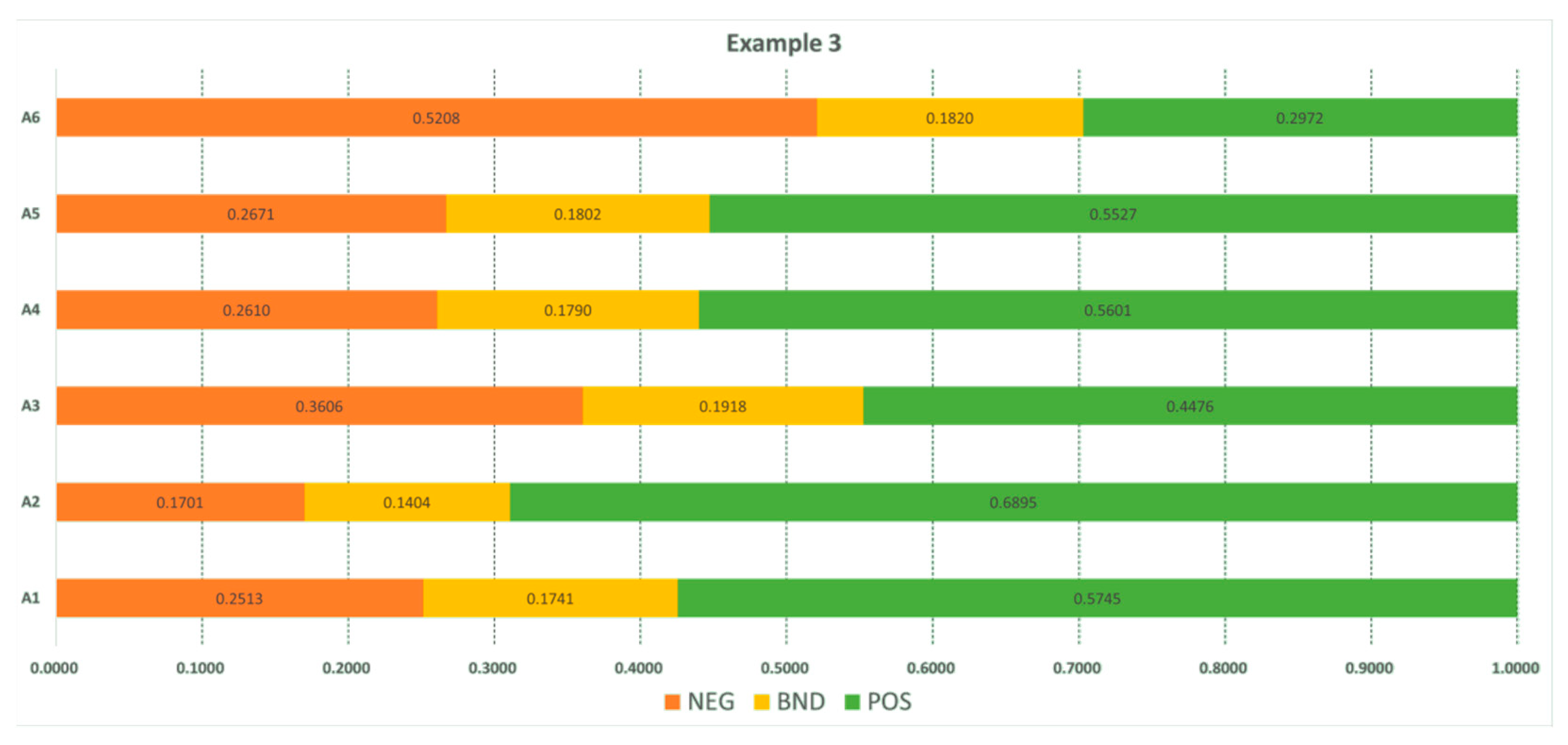
Example 3 [28]: 3D Systems Viper & Protogen 18420, 3D Systems Viper & Somos Next, M3 Linear & CL 20-316L, EOSCINT & PA 2200, EOSCINT & PA 3200 GF, and APCAMA2 & Ti6A/4v ELI are six alternative AM machines. The attributes used to select these AM machines are cost (€), roughness ($\mathsf{\mu }\mathrm{m}$), build time (hrs), strength (MPa), and density (g/cm³).

Table 8. Example 3 $\sigma =\left(0.35, 0.4, 0.4, 0.4, 0.5\right)$.

AM Machine	$\left({\mathit{c}}_1\right)$ Cost	$\left({\mathit{c}}_2\right)$ Roughness	$\left({\mathit{c}}_3\right)$ Build Time	$\left({\mathit{c}}_4\right)$ Strength	$\left({\mathit{c}}_5\right)$ Density
$\left(A_1\right)$ 3D Systems Viper & Protogen 18420	47.70	3.49	5.40	61.38	1.20
$\left(A_2\right)$ 3D Systems Viper & Somos Next	35.08	7.80	2.32	55.10	1.17
$\left(A_3\right)$ M3 Linear & CL 20-316L.	211.42	3.12	6.66	475.00	7.80
$\left(A_4\right)$ EOSCINT & PA 2200	146.14	19.03	3.40	47.22	1.05
$\left(A_5\right)$ EOSCINT & PA 3200 GF	146.14	19.81	3.40	37.92	1.32
$\left(A_6\right)$ APCAMA2 & Ti6A/4v ELI	481.78	24.96	9.02	936.60	4.42

lists the alternative AM machines and the attributes considered for each alternative. The weights of the five attributes are 0.15, 0.15, 0.50, 0.10, and 0.10.

Example 4 [42]: Fortus 360 mc, Fortus 450 mc, Fortus 900 mc, Sigma R17, Sigmax, and Replicator Z18 are six alternative AM machines. The attributes used to select these AM machines are total cost ($), total build time (hrs), and accuracy performance (mm).

Table 9. Example 4 $\sigma =\left(0.35, 0.4, 0.4\right)$.

AM Machine	$\left({\mathit{c}}_1\right)$ Total Cost	$\left({\mathit{c}}_2\right)$ Total Build Time	$\left({\mathit{c}}_3\right)$ Accuracy Performance
$\left(A_1\right)$ Fortus 360 mc	24,923	3807	0.21
$\left(A_2\right)$ Fortus 450 mc	15,314	1531	0.21
$\left(A_3\right)$ Fortus 900 mc	4140	353	0.20
$\left(A_4\right)$ Sigma R17	11,081	2757	1.56
$\left(A_5\right)$ Sigmax	3418	623	1.56
$\left(A_6\right)$ Replicator Z18	32,379	9501	1.66

lists the alternative AM machines and the attributes considered for each alternative. The weights of the three attributes are 0.6700, 0.2475, and 0.0825.

Using the proposed approach, the AM machine selection problems in the above four examples can be solved. As an example, the AM machine selection problem in Example 1 is solved via the eight specific steps of the proposed approach. The intermediate and final results are as follows:

A total of 36 object property assertions are created. By executing the attribute values with the automatic generation program, the DL ontology will automatically generate 36 data property assertions. The results are shown in Figure 3.

A decision matrix $M$ is established as:

$$M=\left[\begin{array}{c}\begin{array}{ccccccc}1800& 53& 100& 1.016& 6& 25.44& 77.78\\ 600& 21& 95& 0.3& 10& 41.47& 1150.18\\ 1430& 50& 100& 1.2& 10& 10.41& 315.03\\ 1703& 53& 100& 0.762& 6& 5.03& 145.51\\ 2000& 60& 99.5& 0.15& 10& 27.45& 679.15\\ 606& 15& 100& 0.6& 10& 41.47& 453.27\end{array}\end{array}\right]$$

A fuzzy decision matrix $M^{{}^{\prime }}$ is established as:

$$M^{{}^{\prime }}=\left[\begin{array}{c}\begin{array}{ccccccc}\langle 0.5009\rangle & \langle 0.4763\rangle & \langle 0.4120\rangle & \langle 0.5411\rangle & \langle 0.2762\rangle & \langle 0.3607\rangle & \langle 0.0535\rangle \\ \langle 0.1670\rangle & \langle 0.1887\rangle & \langle 0.3914\rangle & \langle 0.1598\rangle & \langle 0.4603\rangle & \langle 0.5880\rangle & \langle 0.7907\rangle \\ \langle 0.3980\rangle & \langle 0.4493\rangle & \langle 0.4120\rangle & \langle 0.6391\rangle & \langle 0.4603\rangle & \langle 0.1476\rangle & \langle 0.2166\rangle \\ \langle 0.4739\rangle & \langle 0.4763\rangle & \langle 0.4120\rangle & \langle 0.4058\rangle & \langle 0.2762\rangle & \langle 0.0713\rangle & \langle 0.1000\rangle \\ \langle 0.5566\rangle & \langle 0.5392\rangle & \langle 0.4099\rangle & \langle 0.0799\rangle & \langle 0.4603\rangle & \langle 0.3892\rangle & \langle 0.4669\rangle \\ \langle 0.1686\rangle & \langle 0.1348\rangle & \langle 0.4120\rangle & \langle 0.3196\rangle & \langle 0.4603\rangle & \langle 0.5880\rangle & \langle 0.3116\rangle \end{array}\end{array}\right]$$

A normalized fuzzy decision matrix $M^{{}^{″}}$ is established as:

$$M^{{}^{″}}=\left[\begin{array}{c}\begin{array}{ccccccc}\langle 0.5009\rangle & \langle 0.4763\rangle & \langle 0.5880\rangle & \langle 0.5411\rangle & \langle 0.2762\rangle & \langle 0.6393\rangle & \langle 0.9465\rangle \\ \langle 0.1670\rangle & \langle 0.1887\rangle & \langle 0.6086\rangle & \langle 0.1598\rangle & \langle 0.4603\rangle & \langle 0.4120\rangle & \langle 0.2093\rangle \\ \langle 0.3980\rangle & \langle 0.4493\rangle & \langle 0.5880\rangle & \langle 0.6391\rangle & \langle 0.4603\rangle & \langle 0.8524\rangle & \langle 0.7834\rangle \\ \langle 0.4739\rangle & \langle 0.4763\rangle & \langle 0.5880\rangle & \langle 0.4058\rangle & \langle 0.2762\rangle & \langle 0.9287\rangle & \langle 0.9000\rangle \\ \langle 0.5566\rangle & \langle 0.5392\rangle & \langle 0.5901\rangle & \langle 0.0799\rangle & \langle 0.4603\rangle & \langle 0.6108\rangle & \langle 0.5331\rangle \\ \langle 0.1686\rangle & \langle 0.1348\rangle & \langle 0.5880\rangle & \langle 0.3196\rangle & \langle 0.4603\rangle & \langle 0.4120\rangle & \langle 0.6884\rangle \end{array}\end{array}\right]$$

The relative loss functions are shown in

Table 10. The relative loss functions of Example 1.

		${\mathit{c}}_1$		${\mathit{c}}_2$		${\mathit{c}}_3$		${\mathit{c}}_4$		${\mathit{c}}_6$		${\mathit{c}}_7$
		${\mathit{C}}_1$	$\neg {\mathit{C}}_1$	${\mathit{C}}_2$	$\neg {\mathit{C}}_2$	${\mathit{C}}_3$	$\neg {\mathit{C}}_3$	${\mathit{C}}_4$	$\neg {\mathit{C}}_4$	${\mathit{C}}_6$	$\neg {\mathit{C}}_6$	${\mathit{C}}_7$	$\neg {\mathit{C}}_7$
$A_1$	$a_P$	0	0.4991	0	0.5237	0	0.412	0	0.4589	0	0.7238	0	0.3607
	$a_B$	0.1753	0.1747	0.1905	0.2095	0.2352	0.1648	0.2164	0.1836	0.1381	0.3619	0.2238	0.1262
	$a_N$	0.5009	0	0.4763	0	0.588	0	0.5411	0	0.2762	0	0.6393	0
$A_2$	$a_P$	0	0.833	0	0.8113	0	0.3914	0	0.8402	0	0.5397	0	0.588
	$a_B$	0.0585	0.2916	0.0755	0.3245	0.2434	0.1566	0.0639	0.3361	0.2302	0.2699	0.1442	0.2058
	$a_N$	0.167	0	0.1887	0	0.6086	0	0.1598	0	0.4603	0	0.412	0
$A_3$	$a_P$	0	0.602	0	0.5507	0	0.412	0	0.3609	0	0.5397	0	0.1476
	$a_B$	0.1393	0.2107	0.1797	0.2203	0.2352	0.1648	0.2556	0.1444	0.2302	0.2699	0.2983	0.0517
	$a_N$	0.398	0	0.4493	0	0.588	0	0.6391	0	0.4603	0	0.8524	0
$A_4$	$a_P$	0	0.5261	0	0.5237	0	0.412	0	0.5942	0	0.7238	0	0.0713
	$a_B$	0.1659	0.1841	0.1905	0.2095	0.2352	0.1648	0.1623	0.2377	0.1381	0.3619	0.325	0.025
	$a_N$	0.4739	0	0.4763	0	0.588	0	0.4058	0	0.2762	0	0.9287	0
$A_5$	$a_P$	0	0.4434	0	0.4608	0	0.4099	0	0.9201	0	0.5397	0	0.3892
	$a_B$	0.1948	0.1552	0.2157	0.1843	0.236	0.164	0.032	0.368	0.2302	0.2699	0.2138	0.1362
	$a_N$	0.5566	0	0.5392	0	0.5901	0	0.0799	0	0.4603	0	0.6108	0
$A_6$	$a_P$	0	0.8314	0	0.8652	0	0.412	0	0.6804	0	0.5397	0	0.588
	$a_B$	0.059	0.291	0.0539	0.3461	0.2352	0.1648	0.1278	0.2722	0.2302	0.2699	0.1442	0.2058
	$a_N$	0.1686	0	0.1348	0	0.588	0	0.3196	0	0.4603	0	0.412	0

.

The comprehensive relative loss functions are shown in

Table 11. The comprehensive relative loss functions of Example 1.

		$\mathit{C}$	$\neg \mathit{C}$
$A_1$	$a_P$	0	0.4326
	$a_B$	0.2226	0.1809
	$a_N$	0.5674	0
$A_2$	$a_P$	0	0.6813
	$a_B$	0.132	0.2715
	$a_N$	0.3187	0
$A_3$	$a_P$	0	0.4024
	$a_B$	0.2375	0.1661
	$a_N$	0.5976	0
$A_4$	$a_P$	0	0.3942
	$a_B$	0.2354	0.1681
	$a_N$	0.6058	0
$A_5$	$a_P$	0	0.4697
	$a_B$	0.2115	0.192
	$a_N$	0.5303	0
$A_6$	$a_P$	0	0.5954
	$a_B$	0.1664	0.2372
	$a_N$	0.4046	0

.

The comprehensive thresholds are shown in

Table 12. The comprehensive thresholds of Example 1.

	${\mathit{\alpha }}_{\mathit{i}}$	${\mathit{\beta }}_{\mathit{i}}$
$A_1$	0.5306	0.3442
$A_2$	0.7564	0.5926
$A_3$	0.4988	0.3157
$A_4$	0.4899	0.3122
$A_5$	0.5677	0.376
$A_6$	0.6829	0.4989

.

9.

Make the judgment of each alternative.

The conditional probability $Pr\left(\left.C\right|\left[A_i\right]\right)$ for each alternative is calculated as follows:

$Pr(C|\left[A_1\right])=0.4688$; $Pr(C|\left[A_2\right])=0.4369$; $Pr(C|\left[A_3\right])=0.4761$;

$Pr(C|\left[A_4\right])=0.5083$; $Pr(C|\left[A_5\right])=0.6555$; $Pr(C|\left[A_6\right])=0.4926$;

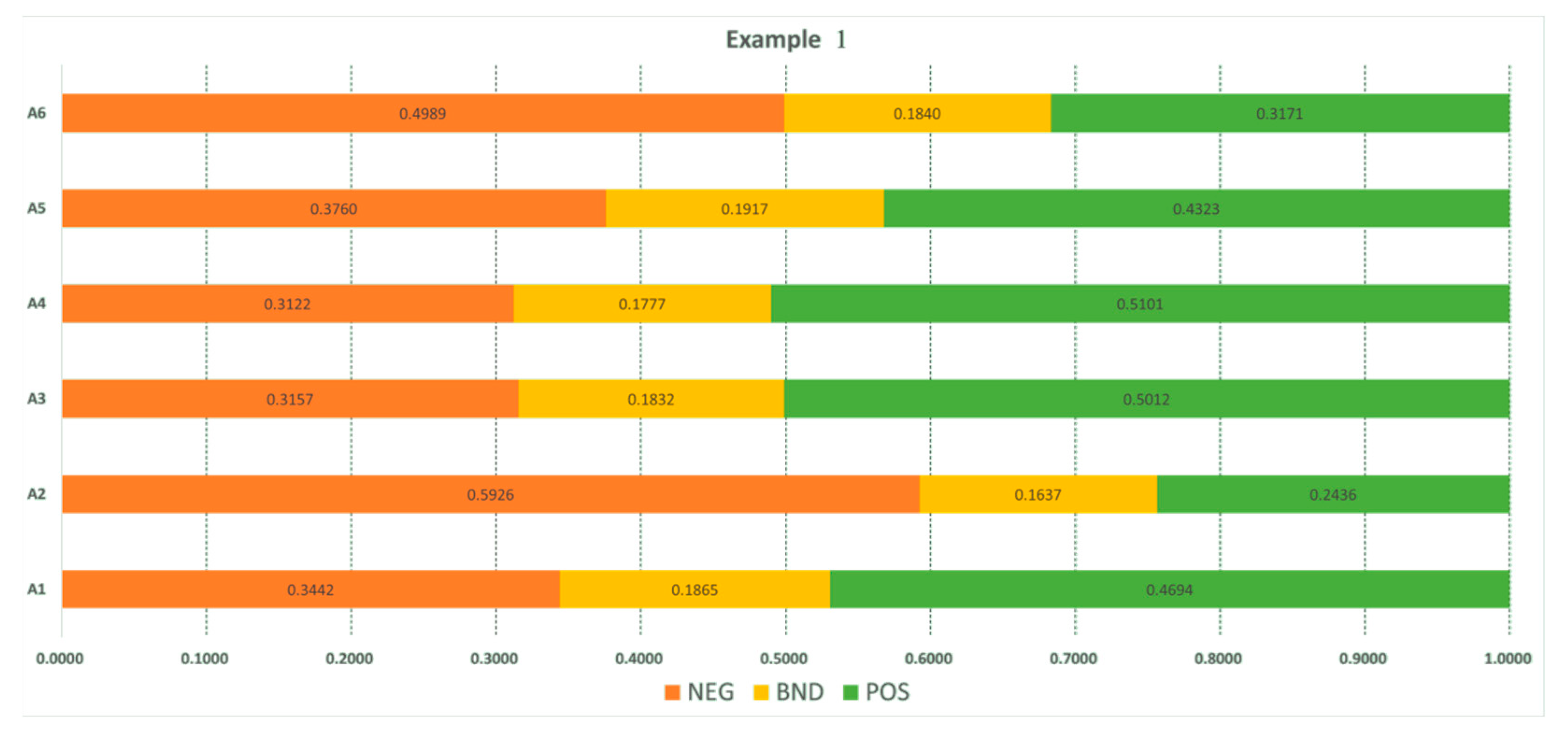
The results of the multi-attribute three-way decisions are shown in Figure 4.

According to the judgment rules (8), (9), and (10), the following judgments are made:

$$NEG\left(C\right)=\left\{A_2, A_6\right\}, BND\left(C\right)=\left\{A_1, A_3\right\}, POS\left(C\right)=\left\{ A_4, A_5\right\}$$

Similarly, the AM machine selection problems in the remaining examples can also be solved using the proposed approach. The results are respectively depicted in Figure 5, Figure 6 and Figure 7. According to the judgment rules (8), (9), and (10), the following judgments are made:

$$\begin{array}{l}\mathbf{Example} \mathbf{2}\mathbf{:} NEG\left(C\right)=\left\{\varnothing \right\}, BND\left(C\right)=\left\{A_3\right\}, POS\left(C\right)=\left\{ A_1, A_2, A_4, A_5, A_6\right\}\\ \mathbf{Example} \mathbf{3}\mathbf{:} NEG\left(C\right)=\left\{A_6\right\}, BND\left(C\right)=\left\{A_3\right\}, POS\left(C\right)=\left\{A_1, A_2, A_4, A_5\right\}\\ \mathbf{Example} \mathbf{4}\mathbf{:} NEG\left(C\right)=\left\{A_6\right\}, BND\left(C\right)=\left\{A_1\right\}, POS\left(C\right)=\left\{A_2, A_3, A_4, A_5\right\}\end{array}$$

4. Demonstration

In this section, two experiments are respectively conducted to demonstrate the effectiveness and advantages of the proposed approach.

4.1. Demonstration of Effectiveness

In general, the effectiveness of a new MADM method is demonstrated by comparing it with existing methods using the same problem. To this end, the four AM machine selection examples listed above are used in the first demonstration experiment. Specifically, Wilson and Rosen [12], Qin et al. [47], and the proposed approach are compared and analyzed using Example 1. Rao and Padmanabhan [14], Vahdani et al. [22], Byun and Lee [10], Zhang and Bernard [28], Zhang et al. [29], Qin et al. [47], and the proposed approach are compared and analyzed using Example 2. Zhang and Bernard [28], Qin et al. [47], and the proposed approach are compared and analyzed using Example 3. Kadkhoda-Ahmadi et al. [42], Qin et al. [47], and the proposed approach are compared and analyzed using Example 4. The experimental results are listed in

Table 13. Results of the comparison experiment.

Example	AM Machine Selection Approach	Generated Rank of Alternative AM Machines
Example 1	Wilson and Rosen [12]	A3 > A5 > A4 > A1 > A6 > A2
	Qin et al. [47]	A3 > A4 > A1 > A5 > A6 > A2
	The proposed approach	$NEG\left(C\right)=\left\{A_2, A_6\right\}$, $BND\left(C\right)=\left\{A_1, A_3\right\}$, $POS\left(C\right)=\left\{ A_4, A_5\right\}$
Example 2	Rao and Padmanabhan [14]	A5 > A1 > A2 > A4 > A3 > A6
	Vahdani et al. [22]	A5 > A1 > A2 > A4 > A3 > A6
	Byun and Lee [10]	A6 > A4 > A5 > A1 > A2 > A3
	Zhang and Bernard [28]	A6 > A5 > A1 > A4 > A2 > A3
	Zhang et al. [29]	A6 > A5 > A4 > A1 > A2 > A3
	Qin et al. [47]	A5 > A1 > A2 > A4 > A3 > A6
	The proposed approach	$NEG\left(C\right)=\left\{\varnothing \right\}$, $BND\left(C\right)=\left\{A_3\right\}$, $POS\left(C\right)=\left\{ A_1, A_2, A_4, A_5, A_6\right\}$
Example 3	Zhang and Bernard [28]	A1 > A2 > A3 > A4 > A5 > A6
	Qin et al. [47]	A2 > A1 > A4 > A5 > A3 > A6
	The proposed approach	$NEG\left(C\right)=\left\{A_6\right\}$, $BND\left(C\right)=\left\{A_3\right\}$, $POS\left(C\right)=\left\{A_1, A_2, A_4, A_5\right\}$
Example 4	Kadkhoda-Ahmadi et al. [42]	A3 > A5 > A2 > A4 > A1 > A6
	Qin et al. [47]	A3 > A5 > A2 > A4 > A1 > A6
	The proposed approach	$NEG\left(C\right)=\left\{A_6\right\}$, $BND\left(C\right)=\left\{A_1\right\}$, $POS\left(C\right)=\left\{A_2, A_3, A_4, A_5\right\}$

.

The experimental results show that:

For Example 1, when the user makes an acceptance decision on two alternatives and a rejection decision on two alternatives, the proposed approach has the same decision results as Wilson and Rosen [12] and Qin et al. [47] in terms of rejection decision, which also shows its effectiveness. However, the decision results of the proposed approach are slightly different from the decision results generated by Wilson and Rosen [12] and Qin et al. [47] in terms of acceptance and noncommitment decisions.

For Example 2, when the user makes an acceptance decision on five alternatives and a rejection decision on zero alternatives, the proposed approach has the same decision results as Byun and Lee [10], Zhang and Bernard [28], and Zhang et al. [29], which verifies its effectiveness. However, the decision results of the proposed approach are slightly different from the decision results generated by Rao and Padmanabhan [14], Vahdani et al. [22], and Qin et al. [47].

For Example 3, when the user an acceptance decision on four alternatives and a rejection decision on one alternative, the proposed approach has the same decision results as Qin et al. [47], which verifies its effectiveness. However, the decision results of the proposed approach are slightly different from the decision results generated by Zhang and Bernard [28].

For Example 4, when the user makes an acceptance decision on four alternatives and a rejection decision on one alternative, the proposed approach has the same decision results as Kadkhoda-Ahmadi et al. [42] and Qin et al. [47], which also shows its effectiveness.

It is worth noting that the main factors that account for the slight differences above include the size of the risk coefficients ${\sigma }_j$, the calculation method of conditional probability $Pr(C|A_i)$, etc.

4.2. Demonstration of Advantages

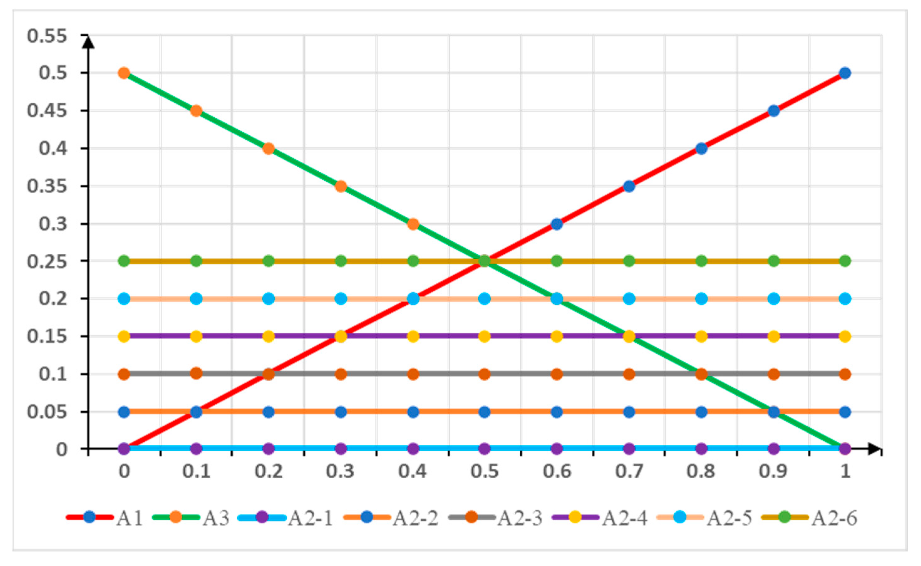
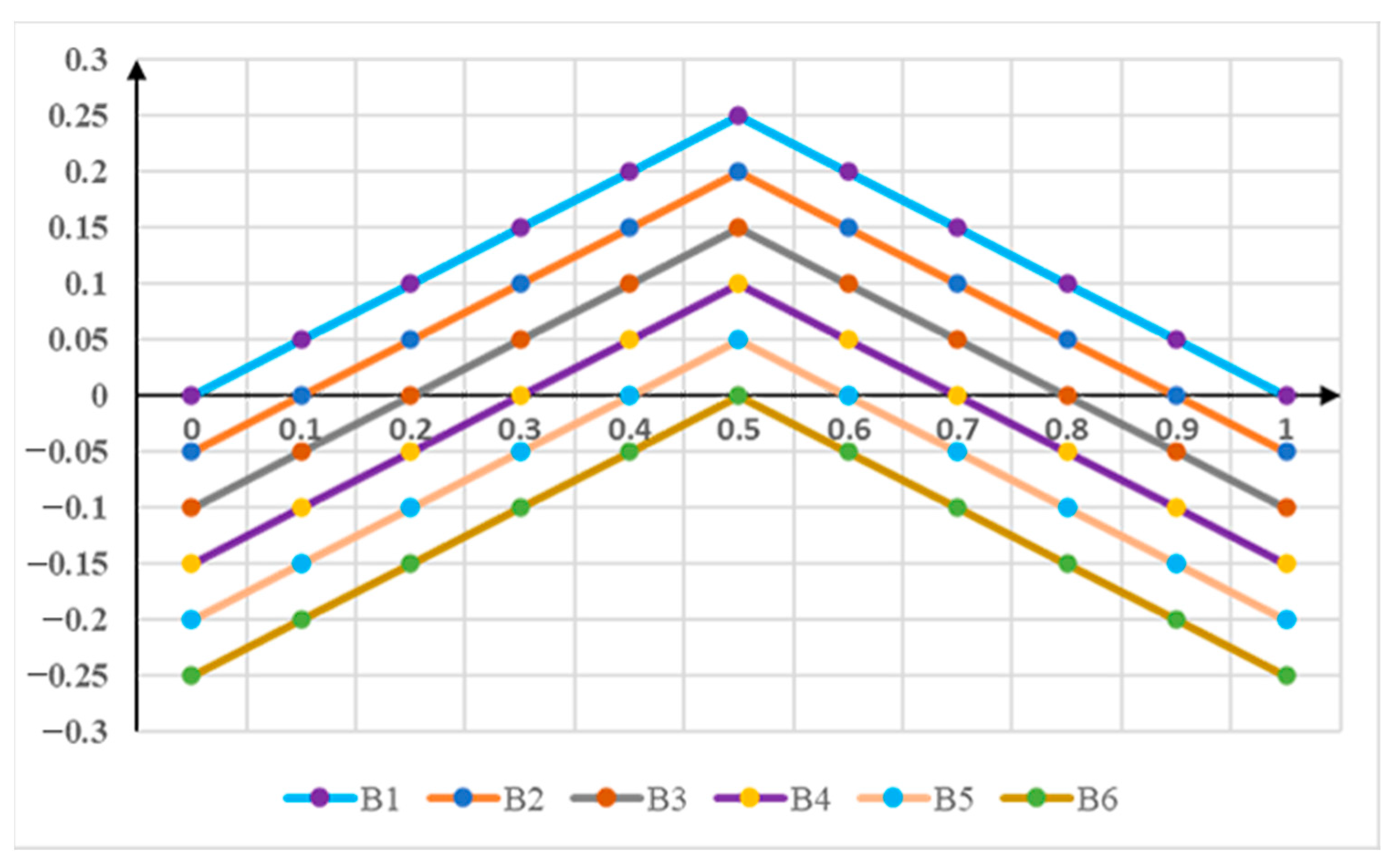
$\sigma$ is called the risk coefficient, which indicates the extent to which a user obtains information. The larger the $\sigma$ value, the more sufficient the information obtained. The second demonstration experiment will demonstrate that the proposed approach is superior to the approaches based on multi-attribute two-way decisions when the $\sigma$ value is small. According to Table 3 and (3), (4), and (5), and assuming $Pr(C|\left[x\right])=0.5$, then the expected loss values of decision $POS\left(C\right)$ (i.e., $a_P$), $BND\left(C\right)$ (i.e., $a_B$), and $NEG\left(C\right)$ (i.e., $a_N$) are, respectively:

$$\begin{array}{l}\mathrm{A}1: R(a_N|\left[x\right])=0.5x_{ij}\\ \mathrm{A}2: R(a_B|\left[x\right])=0.5\sigma \\ \mathrm{A}2\text{-}1: (\mathrm{A}2 \mathrm{curve} \mathrm{at} \sigma =0);\mathrm{A}2\text{-}2: (\mathrm{A}2 \mathrm{curve} \mathrm{at} \sigma =0.1);\\ \mathrm{A}2\text{-}3: (\mathrm{A}2 \mathrm{curve} \mathrm{at} \sigma =0.2);\mathrm{A}2\text{-}4: (\mathrm{A}2 \mathrm{curve} \mathrm{at} \sigma =0.3);\\ \mathrm{A}2\text{-}5: (\mathrm{A}2 \mathrm{curve} \mathrm{at} \sigma =0.4);\mathrm{A}2\text{-}6: (\mathrm{A}2 \mathrm{curve} \mathrm{at} \sigma =0.5);\\ \mathrm{A}3: R(a_P|\left[x\right])=0.5\left(1-x_{ij}\right)\end{array}$$

The dominant values of decision $a_B$ under different $\sigma$ are, respectively:

$$\begin{gathered} \mathrm{B}1: R(a_N|\left[x\right])-R(a_B|\left[x\right]) \mathrm{when} x_{ij}\in \left[0, 0.5\right] \\ R(a_P|\left[x\right])-R(a_B|\left[x\right]) \mathrm{when} x_{ij}\in \left[0.5, 1\right]; (\sigma =0) \\ \mathrm{B}2: R(a_N|\left[x\right])-R(a_B|\left[x\right]) \mathrm{when} x_{ij}\in \left[0, 0.5\right] \\ R(a_P|\left[x\right])-R(a_B|\left[x\right]) \mathrm{when} x_{ij}\in \left[0.5, 1\right]; (\sigma =0.1) \\ \mathrm{B}3: R(a_N|\left[x\right])-R(a_B|\left[x\right]) \mathrm{when} x_{ij}\in \left[0, 0.5\right] \\ R(a_P|\left[x\right])-R(a_B|\left[x\right]) \mathrm{when} x_{ij}\in \left[0.5, 1\right]; (\sigma =0.2) \\ \mathrm{B}4: R(a_N|\left[x\right])-R(a_B|\left[x\right]) \mathrm{when} x_{ij}\in \left[0, 0.5\right] \\ R(a_P|\left[x\right])-R(a_B|\left[x\right]) \mathrm{when} x_{ij}\in \left[0.5, 1\right]; (\sigma =0.3) \\ \mathrm{B}5: R(a_N|\left[x\right])-R(a_B|\left[x\right]) \mathrm{when} x_{ij}\in \left[0, 0.5\right] \\ R(a_P|\left[x\right])-R(a_B|\left[x\right]) \mathrm{when} x_{ij}\in \left[0.5, 1\right]; (\sigma =0.4) \\ \mathrm{B}6: R(a_N|\left[x\right])-R(a_B|\left[x\right]) \mathrm{when} x_{ij}\in \left[0, 0.5\right] \\ R(a_P|\left[x\right])-R(a_B|\left[x\right]) \mathrm{when} x_{ij}\in \left[0.5, 1\right]; (\sigma =0.5) \end{gathered}$$

The experimental results are shown in Figure 8 and Figure 9.

The results show that when $0.5\sigma$ falls below the A1 line (when $x_{ij}\in \left[0, 0.5\right]$) or 0.5$\sigma$ falls below the A3 line (when $x_{ij}\in \left[0.5, 1\right]$), $min(R(a_P|\left[x\right]), R(a_B|\left[x\right]), R(a_N|\left[x\right]))=R(a_B|\left[x\right])$, and the smaller the $\sigma$ value (i.e., the more insufficient the information obtained or the cost for undesirable decision results is high), the larger the dominant value and dominant range ($x_{ij}$ interval corresponding to the dominant value) of decision $a_B$, so it is more flexible and reasonable to make three decisions (i.e., $POS\left(C\right)$, $NEG\left(C\right)$, $BND\left(C\right)$) than to make two decisions (i.e., $POS\left(C\right)$, $NEG\left(C\right)$).

To sum up, the proposed approach has two advantages. First, the proposed approach uses DL ontology to automatically generate attribute values, which is more intelligent and convenient than the traditional ways of obtaining attribute values. Second, it is based on multi-attribute three-way decisions, which are more flexible and reasonable than the traditional multi-attribute two-way decisions, especially when the information obtained for decision making is insufficient. When the information obtained is sufficient, by assigning $\sigma =0.5$, the multi-attribute three-way decisions will transform into multi-attribute two-way decisions.

5. Conclusions

This paper develops an AM machine selection approach based on ontology-supported multi-attribute three-way decisions. This approach consists of two parts. The first part is a DL ontology for AM machine selection, which automatically generates the values of attributes according to the AM machines to be selected and the attributes to be considered. The second part is a decision-making method based on multi-attribute three-way decisions, which prioritizes the alternative AM machines based on the generated attribute values. The paper also illustrates the application of the approach via four AM machine selection examples and demonstrates the effectiveness and advantages of the approach via two experiments. The demonstration results show that that the developed approach is as effective as the existing approaches and the smaller the $\sigma$ value (i.e., the more insufficient the information obtained or the cost for undesirable decision results is high), the larger the dominant value and dominant range ($x_{ij}$ interval corresponding to the dominant value) of decision $a_B$, so it is more flexible and reasonable to make three decisions (i.e., $POS\left(C\right)$, $NEG\left(C\right)$, $BND\left(C\right)$) than to make two decisions (i.e., $POS\left(C\right)$, $NEG\left(C\right)$).

A main limitation of the proposed method is that inappropriate risk coefficients ${\sigma }_j$ may cause no or many alternatives to be classified into the acceptance region, thus making further decisions difficult. In the proposed method, the risk coefficients ${\sigma }_j$ were manually assigned according to experience. It would be of importance to develop an automatic approach to determine proper risk coefficients ${\sigma }_j$. Another limitation is that distortions of the input data may have negative influence the final decision-making results. It would be of necessity to study the reduction of such influence. Last, future work will also focus on applications of the developed approach to other MADM problems in the field of AM, such as material selection, build direction determination, and process parameter optimization. More criteria relevant to part performance would be considered in these applications.

References

- Additive Manufacturing: General: Principles: Terminology; International Organization for Standardization: Geneva, Switzerland, 2015.
- Kumar, L.J.; Pandey, P.M.; Wimpenny, D.I. 3D Printing and Additive Manufacturing Technologies; Springer: Berlin/Heidelberg, Germany, 2019. [Google Scholar]
- Gao, W.; Zhang, Y.; Ramanujan, D.; Ramani, K.; Chen, Y.; Williams, C.B.; Wang, C.C.L.; Shin, Y.C.; Zhang, S.; Zavattieri, P.D. The Status, Challenges, and Future of Additive Manufacturing in Engineering. Comput.—Aided Des. 2015, 69, 65–89. [Google Scholar] [CrossRef]
- Additive Manufacturing: General Principles. Part. 2: Overview of Process Categories and Feedstock; International Organization for Standardization: Geneva, Switzerland, 2015.
- Senvol, L.L.C. Senvol Database: Industrial Additive Manufacturing Machines and Materials. Available online: http://senvol.com/machine-search/ (accessed on 1 January 2023).
- Wang, Y.; Blache, R.; Xu, X. Selection of Additive Manufacturing Processes. Rapid Prototyp. J. 2017, 23, 434–447. [Google Scholar] [CrossRef]
- ISO 17296-3; Additive Manufacturing—General Principles—Part 3: Main Characteristics and Corresponding Test Methods. International Organization for Standardization: Geneva, Switzerland, 2017.
- Braglia, M.; Petroni, A. A Management-Support Technique for the Selection of Rapid Prototyping Technologies. J. Ind. Technol. 1999, 15, 2–6. [Google Scholar]
- Xu, F.; Wong, Y.S.; Loh, H.T. Toward Generic Models for Comparative Evaluation and Process Selection in Rapid Prototyping and Manufacturing. J. Manuf. Syst. 2001, 19, 283–296. [Google Scholar] [CrossRef]
- Byun, H.S.; Lee, K.H. A Decision Support System for the Selection of a Rapid Prototyping Process Using the Modified Topsis Method. Int. J. Adv. Manuf. Technol. 2005, 26, 1338–1347. [Google Scholar] [CrossRef]
- Mahesh, M.; Fuh, J.Y.; Wong, Y.S.; Loh, H.T. Benchmarking for Decision Making in Rapid Prototyping Systems. In Proceedings of the IEEE International Conference on Automation Science and Engineering, Edmonton, AB, Canada, 1–2 August 2005. [Google Scholar]
- Wilson, J.O.; Rosen, D. Selection for Rapid Manufacturing Under Epistemic Uncertainty. In Proceedings of the International Design Engineering Technical Conferences and Computers and Information in Engineering Conference, Long Beach, CA, USA, 24–28 September 2005. [Google Scholar]
- Lan, H.; Ding, Y.; Hong, J. Decision Support System for Rapid Prototyping Process Selection through Integration of Fuzzy Synthetic Evaluation and an Expert System. Int. J. Prod. Res. 2005, 43, 169–194. [Google Scholar] [CrossRef]
- Rao, R.V.; Padmanabhan, K.K. Rapid Prototyping Process Selection Using Graph Theory and Matrix Approach. J. Mater. Process. Technol. 2007, 194, 81–88. [Google Scholar] [CrossRef]
- Armillotta, A. Selection of Layered Manufacturing Techniques by an Adaptive Ahp Decision Model. Robot. Comput. Integr. Manuf. 2008, 24, 450–461. [Google Scholar] [CrossRef]
- Borille, A.; Gomes, J.; Meyer, R.; Grote, K. Applying Decision Methods to Select Rapid Prototyping Technologies. Rapid Prototyp. J. 2010, 16, 50–62. [Google Scholar] [CrossRef]
- Lokesh, K.; Jain, P. Selection of Rapid Prototyping Technology. Adv. Prod. Eng. Manag. 2010, 5, 75–84. [Google Scholar]
- Venkata Rao, R.; Patel, B.K. Decision Making in the Manufacturing Environment Using an Improved Promethee Method. Int. J. Prod. Res. 2010, 48, 4665–4682. [Google Scholar] [CrossRef]
- Zhou, B.; Chen, C. Multi-Level Fuzzy Comprehensive Evaluations for Rapid Manufacturing Systems. In Proceedings of the 2010 Seventh International Conference on Fuzzy Systems and Knowledge Discovery, Yantai, China, 10–12 August 2010. [Google Scholar]
- Chakraborty, S. Applications of the Moora Method for Decision Making in Manufacturing Environment. Int. J. Adv. Manuf. Technol. 2011, 54, 1155–1166. [Google Scholar] [CrossRef]
- Khrais, S.; Al-Hawari, T.; Al-Araidah, O. A Fuzzy Logic Application for Selecting Layered Manufacturing Techniques. Expert Syst. Appl. 2011, 38, 10286–10291. [Google Scholar] [CrossRef]
- Vahdani, B.; Mousavi, S.M.; Tavakkoli-Moghaddam, R. Group Decision Making Based On Novel Fuzzy Modified Topsis Method. Appl. Math. Model. 2011, 35, 4257–4269. [Google Scholar] [CrossRef]
- İç, Y.T. An Experimental Design Approach Using Topsis Method for the Selection of Computer-Integrated Manufacturing Technologies. Robot. Robot. Comput.—Integr. Manuf. 2012, 28, 245–256. [Google Scholar] [CrossRef]
- Mahapatra, S.S.; Panda, B.N. Benchmarking of Rapid Prototyping Systems Using Grey Relational Analysis. Int. J. Serv. Oper. Manag. 2013, 16, 460–477. [Google Scholar] [CrossRef]
- Roberson, D.A.; Espalin, D.; Wicker, R.B. 3D Printer Selection: A Decision-Making Evaluation and Ranking Model. Virtual Phys. Prototyp. 2013, 8, 201–212. [Google Scholar] [CrossRef]
- Liao, S.; Wu, M.J.; Huang, C.Y.; Kao, Y.S.; Lee, T.H. Evaluating and Enhancing Three-Dimensional Printing Service Providers for Rapid Prototyping Using the Dematel Based Network Process and Vikor. Math. Probl. Eng. 2014, 2014, 349348. [Google Scholar] [CrossRef] [Green Version]
- Vinodh, S.; Nagaraj, S.; Girubha, J. Application of Fuzzy Vikor for Selection of Rapid Prototyping Technologies in an Agile Environment. Rapid Prototyp. J. 2014, 20, 523–532. [Google Scholar] [CrossRef]
- Zhang, Y.; Bernard, A. An Integrated Decision-Making Model for Multi-Attributes Decision-Making (Madm) Problems in Additive Manufacturing Process Planning. Rapid Prototyp. J. 2014, 20, 377–389. [Google Scholar] [CrossRef]
- Zhang, Y.; Xu, Y.; Bernard, A. A New Decision Support Method for the Selection of Rp Process: Knowledge Value Measuring. Int. J. Comput. Integr. Manuf. 2014, 27, 747–758. [Google Scholar] [CrossRef]
- Mançanares, C.G.; Zancul, E.d.S.; Cavalcante Da Silva, J.; Cauchick Miguel, P.A. Additive Manufacturing Process Selection Based On Parts’ Selection Criteria. Int. J. Adv. Manuf. Technol. 2015, 80, 1007–1014. [Google Scholar] [CrossRef]
- Paul, D.; Agarwal, P.; Mondal, G.; Banerjee, D. A Comparative Analysis of Different Hybrid Mcdm Techniques Considering a Case of Selection of 3D Printers. Manag. Sci. Lett. 2015, 5, 695–708. [Google Scholar] [CrossRef]
- Makhesana, M.A. Application of Improved Complex Proportional Assessment (Copras) Method for Rapid Prototyping System Selection. Rapid Prototyp. J. 2015, 21, 671–674. [Google Scholar] [CrossRef]
- Vimal, K.; Vinodh, S.; Brajesh, P.; Muralidharan, R. Rapid Prototyping Process Selection Using Multi Criteria Decision Making Considering Environmental Criteria and its Decision Support System. Rapid Prototyp. J. 2016, 22, 225–250. [Google Scholar]
- Kumar, V.; Kumar, L.; Haleem, A. Selection of Rapid Prototyping Technology Using an Anp Based Approach. IOSR J. Mech. Civ. Eng. (IOSR-JMCE) 2016, 13, 71–78. [Google Scholar] [CrossRef]
- Zheng, P.; Wang, Y.; Xu, X.; Xie, S.Q. A Weighted Rough Set Based Fuzzy Axiomatic Design Approach for the Selection of Am Processes. Int. J. Adv. Manuf. Technol. 2017, 91, 1977–1990. [Google Scholar] [CrossRef]
- çetİnkaya, C.; Kabak, M.; Özceylan, E. 3D Printer Selection by Using Fuzzy Analytic Hierarchy Process and Promethee. Bilişim Teknolojileri Dergisi 2017, 10, 371–380. [Google Scholar] [CrossRef] [Green Version]
- Gitinavard, H.; Mousavi, S.M.; Vahdani, B. Soft Computing-Based New Interval-Valued Hesitant Fuzzy Multi-Criteria Group Assessment Method with Last Aggregation to Industrial Decision Problems. Soft Comput. 2017, 21, 3247–3265. [Google Scholar] [CrossRef]
- Anand, M.; Vinodh, S. Application of Fuzzy Ahp–Topsis for Ranking Additive Manufacturing Processes for Microfabrication. Rapid Prototyp. J. 2018, 24, 424–435. [Google Scholar]
- Zaman, U.K.U.; Rivette, M.; Siadat, A.; Mousavi, S.M. Integrated Product-Process Design: Material and Manufacturing Process Selection for Additive Manufacturing Using Multi-Criteria Decision Making. Robot. Comput.—Integr. Manuf. 2018, 51, 169–180. [Google Scholar] [CrossRef] [Green Version]
- Wang, Y.; Zhong, R.Y.; Xu, X. A Decision Support System for Additive Manufacturing Process Selection Using a Hybrid Multiple Criteria Decision-Making Method. Rapid Prototyp. J. 2018, 24, 1544–1553. [Google Scholar] [CrossRef]
- Yildiz, A.; Uğur, L. Evaluation of 3D Printers Used in Additive Manufacturing by Using Interval Type-2 Fuzzy Topsis Method. J. Eng. Res. Appl. Sci. 2018, 7, 984–993. [Google Scholar]
- Kadkhoda-Ahmadi, S.; Hassan, A.; Asadollahi-Yazdi, E. Process and Resource Selection Methodology in Design for Additive Manufacturing. Int. J. Adv. Manuf. Technol. 2019, 104, 2013–2029. [Google Scholar] [CrossRef]
- Moiduddin, K.; Mian, S.H.; Alkhalefah, H.; Umer, U. Decision Advisor Based On Uncertainty Theories for the Selection of Rapid Prototyping System. J. Intell. Fuzzy Syst. 2019, 37, 3897–3923. [Google Scholar] [CrossRef]
- Prabhu, S.R.; Ilangkumaran, M. Decision Making Methodology for the Selection of 3D Printer Under Fuzzy Environment. Int. J. Mater. Prod. Technol. 2019, 59, 239–252. [Google Scholar] [CrossRef]
- Prabhu, S.R.; Ilangkumaran, M. Selection of 3D Printer Based On Fahp Integrated with Gra-Topsis. Int. J. Mater. Prod. Technol. 2019, 58, 155–177. [Google Scholar] [CrossRef]
- Raigar, J.; Sharma, V.S.; Srivastava, S.; Chand, R.; Singh, J. A Decision Support System for the Selection of an Additive Manufacturing Process Using a New Hybrid Mcdm Technique. Sādhanā 2020, 45, 101. [Google Scholar] [CrossRef]
- Qin, Y.; Qi, Q.; Scott, P.J.; Jiang, X. An Additive Manufacturing Process Selection Approach Based on Fuzzy Archimedean Weighted Power Bonferroni Aggregation Operators. Robot. Comput.—Integr. Manuf. 2020, 64, 101926. [Google Scholar] [CrossRef]
- Qin, Y.; Qi, Q.; Shi, P.; Scott, P.J.; Jiang, X. Linguistic Interval-Valued Intuitionistic Fuzzy Archimedean Prioritised Aggregation Operators for Multi-Criteria Decision Making. J. Intell. Fuzzy Syst. 2020, 38, 4643–4666. [Google Scholar] [CrossRef]
- Qin, Y.; Cui, X.; Huang, M.; Zhong, Y.; Tang, Z.; Shi, P. Linguistic Interval-Valued Intuitionistic Fuzzy Archimedean Power Muirhead Mean Operators for Multiattribute Group Decision-Making. Complexity 2020, 2020, 2373762. [Google Scholar] [CrossRef]
- Liu, W.; Zhu, Z.; Ye, S. A Decision-Making Methodology Integrated in Product Design for Additive Manufacturing Process Selection. Rapid Prototyp. J. 2020, 26, 895–909. [Google Scholar] [CrossRef]
- Prabhu, S.R.; Ilangkumaran, M.; Mohanraj, T. 3D Printing of Automobile Spoilers Using Mcdm Techniques. Mater. Test. 2020, 62, 1121–1125. [Google Scholar] [CrossRef]
- Bikas, H.; Porevopoulos, N.; Stavropoulos, P. A Decision Support Method for Knowledge-Based Additive Manufacturing Process Selection. Procedia CIRP 2021, 104, 1650–1655. [Google Scholar] [CrossRef]
- Saxena, P.; Pagone, E.; Salonitis, K.; Jolly, M.R. Sustainability Metrics for Rapid Manufacturing of the Sand Casting Moulds: A Multi-Criteria Decision-Making Algorithm-Based Approach. J. Clean. Prod. 2021, 311, 127506. [Google Scholar] [CrossRef]
- Ransikarbum, K.; Khamhong, P. Integrated Fuzzy Analytic Hierarchy Process and Technique for Order of Preference by Similarity to Ideal Solution for Additive Manufacturing Printer Selection. J. Mater. Eng. Perform. 2021, 30, 6481–6492. [Google Scholar] [CrossRef]
- Psarommatis, F.; Vosniakos, G. Systematic Development of a Powder Deposition System for an Open Selective Laser Sintering Machine Using Analytic Hierarchy Process. J. Manuf. Mater. Process. 2022, 6, 22. [Google Scholar] [CrossRef]
- Raja, S.; John Rajan, A.; Praveen Kumar, V.; Rajeswari, N.; Girija, M.; Modak, S.; Vinoth Kumar, R.; Mammo, W.D. Selection of Additive Manufacturing Machine Using Analytical Hierarchy Process. Sci. Program. 2022, 2022, 1596590. [Google Scholar] [CrossRef]
- Raja, S.; Rajan, A.J. A Decision-Making Model for Selection of the Suitable Fdm Machine Using Fuzzy Topsis. Math. Probl. Eng. 2022, 2022, 7653292. [Google Scholar] [CrossRef]
- Chandra, M.; Shahab, F.; Kek, V.; Rajak, S. Selection for Additive Manufacturing Using Hybrid Mcdm Technique Considering Sustainable Concepts. Rapid Prototyp. J. 2022, 28, 1297–1311. [Google Scholar] [CrossRef]
- Qin, Y.; Qi, Q.; Shi, P.; Lou, S.; Scott, P.J.; Jiang, X. Multi-Attribute Decision-Making Methods in Additive Manufacturing: The State of the Art. Processes 2023, 11, 497. [Google Scholar] [CrossRef]
- Gruber, T.R. A Translation Approach to Portable Ontology Specifications. Knowl. Acquis. 1993, 5, 199–220. [Google Scholar] [CrossRef]
- Musen, M.A. The Protégé Project: A Look Back and a Look Forward. AI Matters 2015, 1, 4–12. [Google Scholar] [CrossRef] [Green Version]
- Jia, F.; Liu, P. A Novel Three-Way Decision Model Under Multiple-Criteria Environment. Inf. Sci. 2019, 471, 29–51. [Google Scholar] [CrossRef]
- Yao, Y.; Wong, S.K.M. A Decision Theoretic Framework for Approximating Concepts. Int. J. Man-Mach. Stud. 1992, 37, 793–809. [Google Scholar] [CrossRef]
- Liang, D.; Pedrycz, W.; Liu, D.; Hu, P. Three-Way Decisions Based On Decision-Theoretic Rough Sets Under Linguistic Assessment with the Aid of Group Decision Making. Appl. Soft. Comput. 2015, 29, 256–269. [Google Scholar] [CrossRef]
- Huang, M.; Chen, L.; Zhong, Y.; Qin, Y. A Generic Method for Multi-Criterion Decision-Making Problems in Design for Additive Manufacturing. Int. J. Adv. Manuf. Technol. 2021, 115, 2083–2095. [Google Scholar] [CrossRef]
- Liu, P.; Wang, Y.; Jia, F.; Fujita, H. A Multiple Attribute Decision Making Three-Way Model for Intuitionistic Fuzzy Numbers. Int. J. Approx. Reason. 2020, 119, 177–203. [Google Scholar] [CrossRef]
- Qin, Y.; Qi, Q.; Shi, P.; Scott, P.J.; Jiang, X. A multi-criterion three-way decision-making method under linguistic interval-valued intuitionistic fuzzy environment. J. Ambient Intell. Humaniz. Comput. 2022. [Google Scholar] [CrossRef]
- Qin, Y.; Qi, Q.; Shi, P.; Scott, P.; Jiang, X. Selection of materials in metal additive manufacturing via three-way decision-making. Int. J. Adv. Manuf. Technol. 2023. [Google Scholar] [CrossRef]
Figure 1.
Graphical representation of fifteen top-level concepts in the DL ontology.
Figure 2.
Ontological view of automatic generation of AM machine attribute values.
Figure 3.
Automatic generation of attribute values for Example 1.
Figure 4.
Results of the multi-attribute three-way decisions for Example 1.
Figure 5.
Results of the multi-attribute three-way decisions for Example 2.
Figure 6.
Results of the multi-attribute three-way decisions for Example 3.
Figure 7.
Results of the multi-attribute three-way decisions for Example 4.
Figure 8.
Loss value functions for A1, A2, and A3.
Figure 9.
The dominant value curves of decision under different .