Payload Camera Breadboard for Space Surveillance—Part I: Breadboard Design and Implementation

Abstract

The rapid increase of space debris poses a risk to space activities, so it is vital to develop countermeasures in terms of space surveillance to prevent possible threats. The current Space Surveillance Network is majorly composed of radar and optical telescopes that regularly observe and track space objects. However, these measures are limited by size, being able to detect only a tiny amount of debris. Hence, alternative solutions are essential for securing the future of space activities. Therefore, this paper proposes the design of a payload camera breadboard for space surveillance to increase the information on debris, particularly for the under-catalogued ones. The device was designed with similar characteristics to star trackers of small satellites and CubeSats. Star trackers are attitude devices usually used in satellites for attitude determination and, therefore, have a wide potential role as a major tool for space debris detection. The breadboard was built with commercial off-the-shelf components, representing the current space-camera resolution and field of view. The image sensor was characterized to compute the sensitivity of the camera and evaluate the detectability performance in several simulated positions. Furthermore, the payload camera concept was tested by taking images of the night sky using satellites as proxies of space debris, and a photometric analysis was performed to validate the simulated detectability performance.

1. Introduction

Most space debris observation and tracking are done by the Space Surveillance Network, constituted by a set of over 30 ground-based optical and radar telescopes located worldwide, and six satellites that regularly track objects in orbit and maintain a catalogue of about 32,000 objects. These observations have a size limitation ranging from 10 cm in Low Earth orbit (LEO) to about 1 m in Geostationary Earth orbit (GEO). The catalogued objects represent a tiny amount of the total since statistical-debris environmental models estimate more than 131 million space objects ranging from 1 mm to 10 cm [1,2,3].

Star trackers (STRs) are one of the most accurate attitude sensors developed for modern spacecrafts used to determine the attitude by detecting stars in the STR’s field of view (FOV). STR architecture consists of an optical system, an image sensor, electronics, and a signal-processing system. The optical system is composed of a set of lenses and a light shield called the Baffle, which protects the STR from light that affects its functioning, such as Sunlight. The image sensor, responsible for taking the observed objects’ images, can be a Charge Couple Device (CCD) or a Complementary Metal-Oxide-Semiconductor (CMOS). The drivers and controllers, i.e., electronics and signal processing systems, comprise the processors and software, namely, controllers and drivers that control and operate the hardware [4,5,6,7].

STRs used to be a high-technology device with a high cost. With the advent of New Space activities, new studies that use COTS (Commercial Off-The-Shelf) equipment in STRs to reduce the size and cost have been performed in the last years.

An STR for small satellites and CubeSats should ideally have as high of an accuracy as possible and minimal power consumption, volume, and mass. However, this is hard to obtain. For example, better optics or an image sensor with a higher resolution can improve the STR accuracy. Still, better optics require more volume and, consequently, more mass. A higher-resolution sensor, on the other hand, requires a larger memory and a better processor. Hence, the selection of the components has lower and upper limits to maintain the characteristics of the system [8].

Table 1. STRs with COTS components.

STR	Image Sensor	FOV
CubeStar	Melexis MLX75412 CMOS 1024 × 512 pixels 5.6 µm	42° circular
SOST	Sony IMX219PQ color 8 MPix 3280 × 2464 pixels 1.12 µm	62.2° × 48.8°
APST	MT9P031 CMOS 2592 × 1944 2.2 µm	15° circular

lists some examples of COTS STRs.

Due to good results, CubeStar [9] was developed and implemented in CubeSat missions, and it is commercially sold nowadays. The SOST [10] platform passed the laboratory tests for vibration and thermo-vacuum conditions, but it has not been evaluated in space. APST [6] shows good ground-based observation results, detecting stars up to 5.85 in magnitude. Furthermore, these studies suggest that the lens of an STR should have a low-focal number, in the order of 1.2 to 1.8, to produce bright images. Also, an STR must have a large FOV, varying from 10° to 40°, since this characteristic has advantages like lower memory, less computational time, and moderate accuracy. Lastly, a CMOS sensor is preferable compared to CCDs due to the advantages of lower power consumption, radiation resistance, and lower price.

Besides attitude extraction, some works demonstrate the capability of STRs and space cameras in space-debris detection. Clemens [11] did a feasibility study using a COTS STR to detect resident space objects (RSO) by developing a simulator to evaluate the capability of STR detection. The conclusion shows that a dedicated STR, used only for RSO detection, is feasible and can detect more than 1200 objects/day. However, a dual-purpose STR, a device that extracts the attitude and detects RSOs simultaneously, did not achieve concrete results. Liu et al. [12] propose a feasibility study using a network based on multiple STRs for space-debris detection and monitoring, establishing an algorithm that uses the images taken by STRs on satellites during attitude fixation to detect and extract space targets to increase the available data information of space target surveillance. The study was developed using the characteristics of current STRs in operation since onboard STRs save costs on launching dedicated-surveillance satellites. It demonstrated accurate results for debris detection and orbit determination by STRs. However, it only works for a constellation of satellites.

Feiteirinha et al. [13] did a proof-of-concept study of planned or opportunistic debris observation using STRs when there are available resources like downlink, mass memory, and cameras. The authors used the STRs of the SWARM mission to prove that it is possible to observe RSOs. They also developed a model to automatically request, download, and process the optimal amount of information without impacting the standard operation of the STRs. It was proved that STRs can be used for debris detection when these devices are not extracting the attitude. Kimura et al. [14] developed a highly intelligent camera using COTS devices capable of detecting, tracking, and calculating the orbit position to automatically control the rendezvous for debris removal. The image-processing functions obtained successful test results, and the camera’s orbit-determination function was validated in various simulation conditions. Due to the good results, the system was ready for launch in the ELSA-d satellite to further tests in situ. However, this camera was designed for relatively larger debris detection. Moreover, as the camera system was designed with COTS devices in mind, the authors verified the space-environment tolerance to minimize the costs of development and maximize the performance. The camera was approved in the vibration, thermal, and thermal-vacuum tests and proved to be in-orbit tolerant. In addition, the authors also developed COTS-onboard cameras for the Hayabusa2 spacecraft and the IKAROS mission [15,16], showing that COTS devices can be applied for space applications.

The literature on detecting space debris using space cameras or STRs is extensive and covers different areas of study, and it has been shown that these devices can be used for space surveillance in the scope of space debris. This paper proposes a new solution through the development of a low-cost payload camera similar to STRs using COTS devices for under-catalogued space debris detection. Therefore, the performance of the proposed camera-payload breadboard will be evaluated in terms of detectability to test the size-detection capacity of the device.

This paper adopts the following structure: Section 2 addresses the camera design and implementation; Section 3 presents the experimental methods and results; and Section 4 outlines the conclusions.

2. Breadboard Design and Implementation

The first step in designing an optical device is the study of the intensity of the optical signal, i.e., the radiometric calculations on the optical sensor. Section 2.1 presents the breadboard architecture; in Section 2.2, the characterization of the sensor is proposed; in Section 2.3, the prediction of the limiting magnitude of the sensor, i.e., the radiometric calculation on the camera, is presented; and in Section 2.4, the magnitude of space debris is calculated. Finally, in Section 2.5, the minimally detectable size of debris is determined using the estimated limiting magnitude of the sensor.

2.1. Breadboard Architecture

The architecture of the breadboard consisted of the computer laptop, the camera plus the camera controller, the image sensor, the optics, the temperature sensor, and the temperature controller, as shown in Figure 1.

All components used in implementing the camera breadboard are COTS devices. The selected image sensor was an Aptina MT9J001 monochromatic CMOS sensor of 10 megapixels (MP). This sensor is similar to the one proposed by the APST STR [6]. The specifications of the sensor are presented in

Table 2. Aptina MT9J001 specifications.

Properties	Specification
Active image size	6.440 mm (H) × 4.616 mm (V)
Resolution	3856 × 2764 pixels
Pixel size	1.67 × 1.67 µm
SNRMAX	34 dB

.

The image sensor relates to the Arducam USB2 Camera Shield, which is the camera control board. The sensor is connected to the Arducam by a 30-pin ribbon cable in the secondary camera interface. The chosen lens is a Fujian, with an $f_{number}$ of 1.6, a parameter value suggested by the literature, and a focal length of 35 mm. Therefore, the system’s FOV is given by:

$$FOV=2\left(\frac{\raisebox{1ex}{$h_{sensor}$}\!\left/ \!\raisebox{-1ex}{$2$}\right.}{f}\right)$$

(1)

In (1), $h_{sensor}$ is the sensor’s active image size and $f$ the focal length. Thereby, the FOV of the system is 10.5 deg horizontally and 7.5 deg vertically. Thus, the circular FOV is given by [17]:

$$FO{V}_{circular}=\sqrt{\frac{FO{V}_{horizontal}FO{V}_{vertical}}{\pi }}\times 2$$

(2)

Then, the circular FOV of the camera is about 10 deg, which is within the values recommended by the literature. Moreover, the $f_{number}$, which denotes the photons that cross the lens, is calculated by the ratio between the focal length $f$ and the diameter of the system’s aperture $d$:

$$f_{number}=\frac{f}{d}$$

(3)

Considering (3), it is possible to calculate the lens aperture, which is 22 mm.

• Mechanical design

An optical system is very sensitive, and minimal disturbances can lead to errors in the acquired data. So, a mechanical system was designed to maintain the optics as stable as possible. This mechanical design was done in SolidWorks and then 3D printed. The design was developed to place the optical and temperature systems on the same breadboard. The outcome is shown in Figure 2.

The temperature system is made of aluminium parts produced in a CNC-milling machine. The remaining parts of the platform were 3D printed. The sensor and Arducam are inside the platform. The lens is connected to the sensor by a c-mount adaptor, and the structure that involves the lens has the purpose of fixating the focus. The optical system is connected to a computer, which controls the camera.

The temperature system has a temperature controller, a temperature sensor, a thermoelectric cooler (TEC), a heat sink, and aluminium pieces. The temperature controller is connected to an external power supply and the computer. This device sends a programmed temperature to the TEC, cooling the aluminium pieces and, consequently, the optical sensor. The temperature sensor measures the temperature of the CMOS sensor.

2.2. Sensor Characterisation

The charge conversion efficiency (CCE), readout noise, and sensor’s dark current were characterized. The CCE is related to the electrons’ number converted into digital counts. Therefore, CCE can be calculated using a homogeneous and monochromatic light source. The CCE calculation is done by plotting the images’ variance and mean counts of the light source for several integration times until it reaches saturation. A helium–neon gas laser beam was used as the source of light, which assures a monochromatic light source.

The measurements were done in an integration sphere, ensuring the sensor received a homogeneous light. The used integration sphere had three orifices where any instrument could be installed. The laser used was assembled in one cavity, the sensor in another, and the remaining was closed.

Ten frames were taken, varying from the minimal integration time of $6.31\mathsf{\mu }\mathrm{s}$ up to the completely saturated value, $71.43 \mathrm{ms}$. Then, each frame variance and mean counts were extracted. The region where these two values have an approximate linear behaviour was chosen. The variance-versus-mean-counts linear relation for several images extracted by the MT9J001 with the laser beam switched on are shown in Figure 3. The CCE result is taken from the slope of the data’s linear fit. Therefore, a value of $5.22 \frac{e^{-}}{ADU}$ was found, where the Analog-Digital Units (ADU) represent the pixel reading value.

• Readout noise

The readout noise is measured from a bias frame, an image taken with the shutter closed in the minimum integration time possible (virtually zero seconds). Therefore, the sensor with the shutter closed was mounted in the integration sphere. The other cavities were sealed, and the laboratory lights were turned off. After that, it was extracted two frames in the minimum integration time of $6.31\mathsf{\mu }\mathrm{s}$. Thus, the noise structure was computed by the subtraction of both frames, resulting in a value with the standard deviation of the counts of $\sigma =3.24 \mathrm{ADU}$. The readout noise $N_{RN}$ is then given by:

$$N_{RN}=\frac{CCE \sigma }{\sqrt{2}}$$

(4)

Substituting the results of $\sigma$ and CCE in (4) gives a $N_{RN}=11.97 e^{-}$.

• Dark noise

The dark noise is computed through the dark current, which is measured by taking dark frames, images taken in the dark with the shutter closed, at a controlled temperature. The dark frame uses an integration time that is different from the minimal value, diverging from the bias frame in this aspect.

The dark current was measured in the integration sphere with the aforementioned configuration at a constant temperature of 24 °C. Ten dark frames with several integration times were taken until the sensor reached a moderated level of saturated pixels. Afterwards, a mean of the ten measurements for the different integration times was computed. The mean values obtained for each integration time are shown in Figure 4.

In Figure 4, the slope of the linear fit indicates the dark current: 0.2098 ADU/s. This value can be converted to electrons/s, giving 1.095 e⁻/s. The dark noise $N_{DN}$ is then given by:

$$N_{DN}=\sqrt{i_{DC}t}$$

(5)

In (5), $i_{DC}$ is the dark current, and $t$ is the integration time.

• Focus and FWHM of the optical system

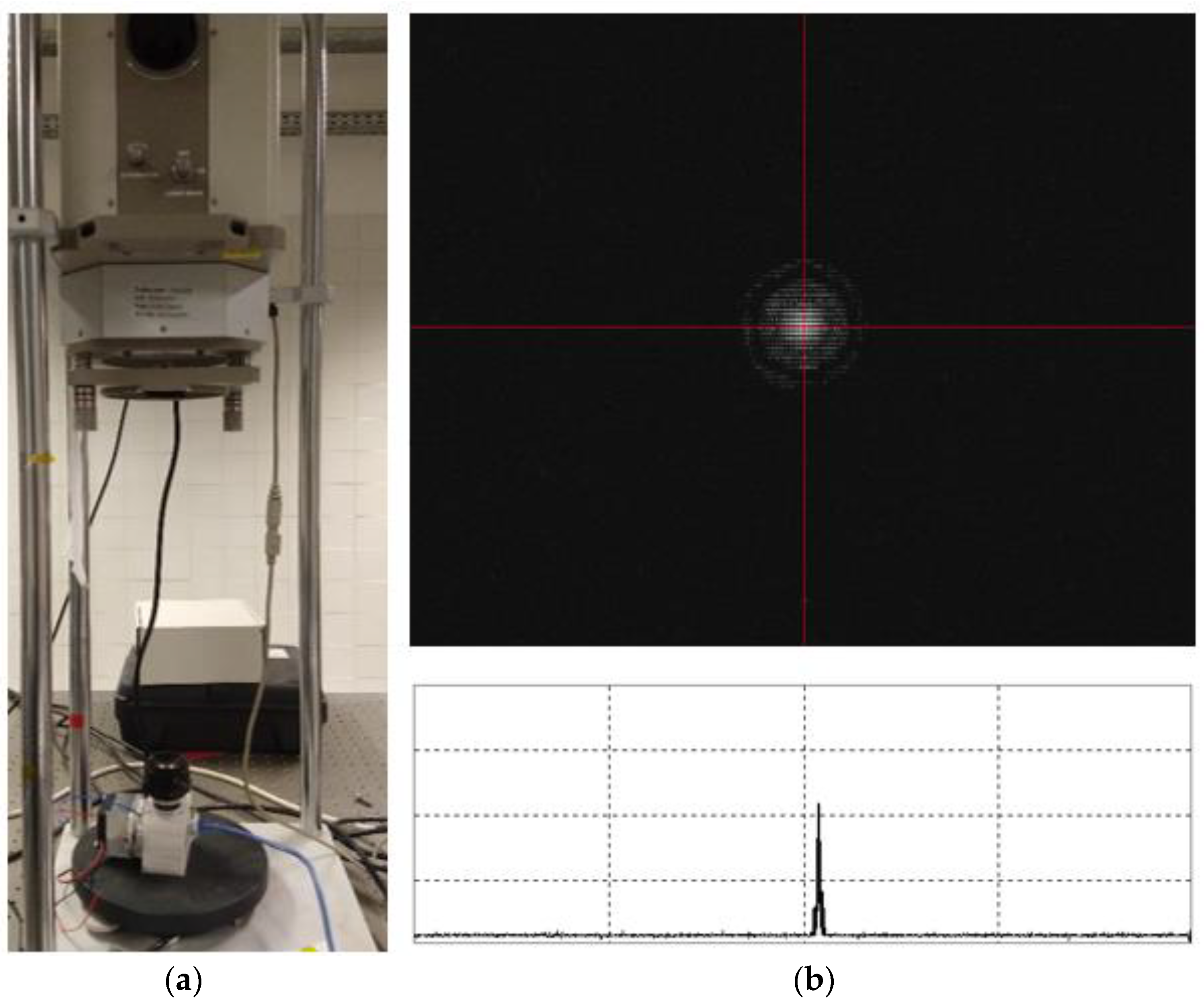
The optical system focus and the full width at half maximum (FWHM) of the signal of a point source were found using an interferometer. The interferometer sends a light beam representing a light source at an infinite distance to the camera. The best configuration for the focus is achieved when the light beam occupies the minimum value of pixels in the sensor, i.e., the minimum FWHM. Figure 5 shows the camera in the interferometer (a) and the image of the focused light beam (b).

After achieving the best result, as seen in Figure 5b, the software ThorCan and SAOImageDS9 were used to determine the number of pixels the light beam signal occupies. A value of 16 pixels was found, also representing the number of pixels an A0-type star occupies in the sensor.

2.3. Estimating the Limiting Magnitude of the Sensor

The limiting magnitude is the maximum threshold value that the sensor can detect, i.e., the minimum brightness. In other words, this magnitude will provide the minimum size of detectable debris. To estimate the limiting magnitude, it is necessary to have information on the sources’ brightness in specific wavebands relative to standard stars and the quantum efficiency of the sensor for different wavelengths.

The Johnson-Cousins filters system was used as the information on the flux calibration of A0-type main-sequence stars for the distinct wavebands that the sensor can detect, namely blue (B), visible (V), red (R), and near-infrared (I) [18]. Also, the spectral sensitivity curve, present in the sensor datasheet [19], provides the values of the sensor quantum efficiency ($QE$) in different wavelengths. Therefore, the A0 star flux ${\mathsf{\Phi }}_0$ measured by the sensor is given by [18]:

$${\mathsf{\Phi }}_0={\displaystyle \sum }_{x=B,V,R,I}{\mathsf{\Phi }}_{x}FWH{M}_{x}Q{E}_{{\lambda }_x}$$

(6)

Thus, the flux is the summation of the flux in different wavebands times the FWHM and quantum efficiency of each waveband as described in (6). After that, the magnitude m is determined by comparing the flux of a standard star, with a well-known magnitude, and the flux of the object of interest:

$$m-m_0=-2.5\log \left(\frac{\mathsf{\Phi }}{{\mathsf{\Phi }}_0}\right)$$

(7)

In (7), the index 0 represents the standard star. Rearranging this equation, the flux for different magnitudes is given by:

$$\mathsf{\Phi }={\mathsf{\Phi }}_0 {10}^{-\frac{m-m_0}{2.5}}$$

(8)

Thus, (8) provides the flux in $\frac{W}{m^2}$ for several values of magnitudes. The flux unit was converted to photons/m² by dividing each waveband flux by its photon energy. Then, our lens’s transmission coefficient, which is 0.7, and its aperture area, as seen in Section 2.1, are multiplied in the outcomes. Hence, the flux has units of photons/s. Therefore, the sensor signal for different magnitudes was obtained by multiplying this result by the integration time. Thereby, signal and total noise values were used to determine the signal-to-noise ratio (SNR) [20]:

$$SNR=\frac{N_{*}}{\sqrt{N_{*}+n_{pix}\left(N_{SN}+N_{DN}+N_{RN}^2\right)}}$$

(9)

In (9), $N_{*}$ is the signal and $n_{pix}$ is the number of pixels considered for the calculation, which was 16 (FWHM calculated in Section 2.2). $N_{SN}$ is the shot noise and is calculated by the square root of the signal. Also, the results estimated in Section 2.2 for the readout noise, $N_{RN}$, and the dark noise, $N_{DN}$, were applied in the SNR calculation.

We considered the canonical SNR = 5 as the reliable detection limit, i.e., a detection is only reliable when its signal is five times higher than the noise levels. Therefore, for three integration times of 1 s, 3 s, and 5 s, the maximum detection magnitudes, i.e., the magnitudes of the faintest detectable objects/stars, were approximately 10.2, 11.4 and 11.9, respectively.

2.4. Visual Magnitude of Debris

The visual magnitude of debris relates to its capability to reflect solar light, which depends on size, phase angle, reflectivity, and the distance between the observer and the debris, known as range. The most common method to estimate the magnitude of an object/debris whose brightness depends only on the light it reflects from the Sun is [11,21,22]:

$$M=m_{sun}-2.5\log \left(\frac{pAF\left(\varphi \right)}{R^2}\right)$$

(10)

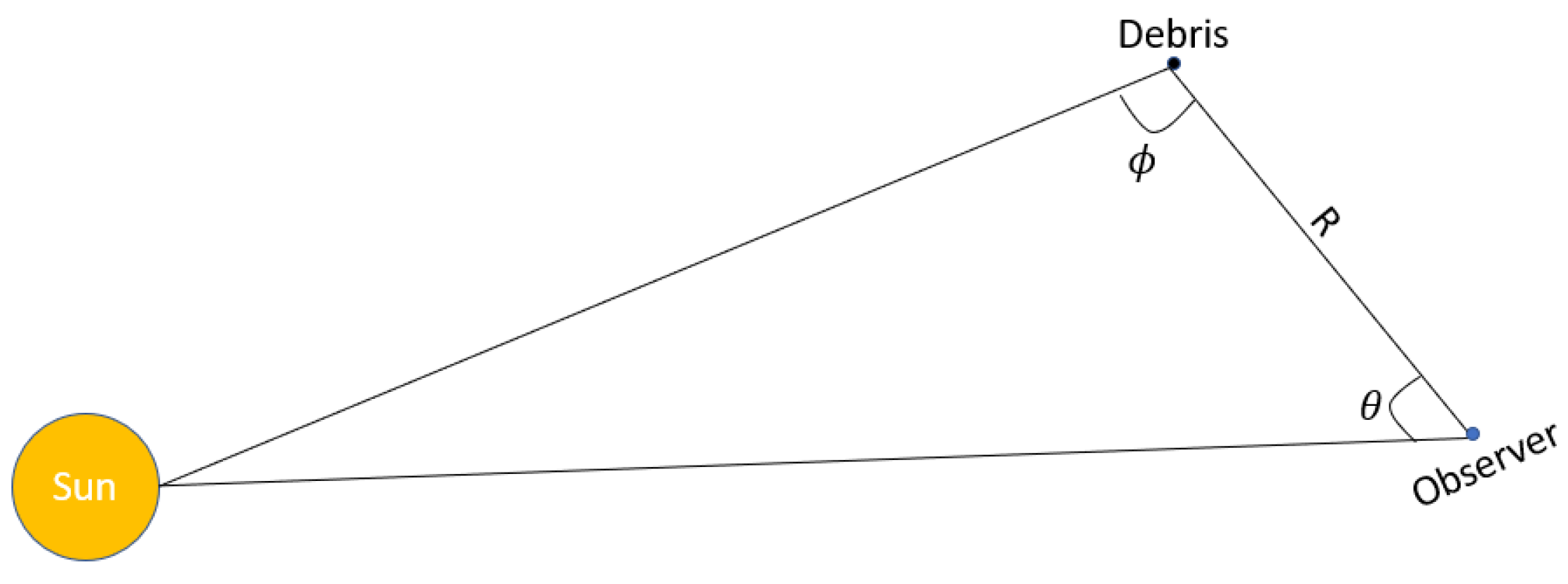
In (10), $m_{sun}$ is the Sun’s visual magnitude, p is the geometric albedo (a specifically quantified form of reflectivity), A is the object cross-section area, R is the distance between the object and the observer/camera (range), and F is the solar-phase angle function, being ϕ the solar-phase angle (i.e., the Sun-object-observer angle as seen in Figure 6). The latest estimation for the average albedo of debris is 0.175 [11]. As a first approximation, the observed object is considered a sphere.

In Figure 6, ϕ is the solar-phase angle, R is the range and θ the Sun-debris angle seen by the observer. The solar-phase angle is related to the illumination condition of an object in space and is defined as the angle between the Sun and the observer seen from the object (in our case, a piece of space debris). Moreover, most of the light reflected by debris is diffuse and not specular. Then, considering an object of unknown shape as an ideal diffusing reflector is a reasonable approximation [21,23,24]. Therefore, the diffuse-phase function for a spherical body is given by:

$$F_{diff}\left(\varphi \right)=\frac{2}{3{\pi }^2}\left[\left(\pi -\varphi \right)\cos \varphi +\sin \varphi \right]$$

(11)

Finally, the solar-phase angle can be calculated by looking at the problem’s geometry. The Sun, the debris, and the observer locations form a triangle in the celestial sphere (see Figure 6). Considering the Horizontal Coordinates of the observer, the Sun-debris angle seen by the observer can be determined by the haversine formula [25], which calculates the angle between two coordinates:

$$\theta =2{\sin }^{-1}\left(\sqrt{{\sin }^2\left(\frac{{\alpha }_{sun}-{\alpha }_{debris}}{2}\right)+\cos {\alpha }_{sun}\cos {\alpha }_{debris}{\sin }^2\left(\frac{A_{sun}-A_{debris}}{2}\right)}\right)$$

(12)

In (12), ${\alpha }_{sun}$ and ${\alpha }_{debris}$ are the elevation of the Sun and the debris, respectively, and $A_{sun}$ and $A_{debris}$, the respective azimuths. Looking again at the triangle Sun-debris-observer, the distance between Sun and debris or Sun and observer is much larger than the range of the debris. Thus, the angle at the corner of the Sun in the triangle is approximately zero. Therefore, the solar phase angle is given by:

$$\varphi =\pi -\theta$$

(13)

Theoretically, the phase angle ranges from 0 deg, representing the best scenario, to 180 deg, the worst illuminated case. However, in practice, the phase angle depends on the observational window, providing a minimal angle higher than 0 deg and a maximal smaller than 180 deg.

2.5. Limiting Magnitude of the Sensor and Visual Magnitude of Debris

The sensor’s limiting magnitude sets its detectability of space debris. In other words, the sensor can only detect objects that reflect enough light, otherwise, they will be under the SNR = 5 threshold for reliable detection. Therefore, different scenarios can be simulated to evaluate the detectability of the camera. Simulations were done considering a spherical debris in a circular orbit of 800 km altitude. After that, the distance between the sensor and the object (range) was changed. Also, the same pessimistic solar-phase angle of $120\mathrm{deg}$ was considered for all the scenarios.

Taking into consideration the limiting magnitude of 10.2 for a fixed source, like a star, at an SNR = 5 and an integration time of 1 s, one would expect to detect the signal of a piece of space debris with the same magnitude. However, space debris are fast-moving objects, and their signal is not integrated over the same pixels but rather spread over its streak. The longer the integration, the longer the streak. For example, a piece of debris orbiting the Earth at an 800 km altitude would have an orbital velocity of $v_{orb}=7.452 \mathrm{km}/\mathrm{s}$, an orbital period of $P_{orb}=6052 \mathrm{s}$, and an angular velocity relative to the Earth center of ${\mathsf{\omega }}_{orb}=214.1 \mathrm{arcsec}/\mathrm{s}$. Its visibility, for an observer on Earth, occurs during an Earth-centered angle of $\mathsf{\psi }=54.617 \mathrm{deg}=196621 \mathrm{arcsec}$. For an observer on the surface of the Earth, and not at its centre, the average sky motion of such object is $\mathsf{\delta }=705.7 \mathrm{arcsec}/\mathrm{s}$.

Since the average pixel scale of our detector is $\mathrm{s}=9.79 \mathrm{arcsec}/\mathrm{pix}$, during a 1 s integration, the debris will trail over 72.1 pixels on the detector, spreading its signal on the streak. While the signal of a fixed point-source is accumulated on 16 pixels, the debris signal will be spread over 342 pixels. Therefore, the maximum magnitude of a piece of space debris on a circular orbit at an altitude of 800 km, detectable at an SNR = 5 with our equipment, for a 1 s exposure is $m=8.6$. For a 3 s exposure, the signal would be spread over 994 pixels, and for 5 s spread over 1651 pixels, resulting in magnitudes of 9.2 and 9.5 respectively.

Analogously, for debris in circular orbits at 1000 km altitude, we get a maximum magnitude of about 8.7, and for circular orbits at 2000 km altitude, we get about 8.9, both for a 1 s exposure. The higher the orbit, the closer to the fixed-star maximum magnitude we get. This apparently counter-intuitive output does not evidently result in a detection of smaller debris at higher altitudes. In order not to leave a streak on the image, a piece of debris would need to be moving at a rate lower than 1 arcsec/s relative to the Earth’s centre, which would mean orbiting at an altitude higher than 200,000 km, an orbit of no immediate interest, and for such distance, only a debris with a diameter larger than about 20 m would be measured with magnitude 10.2 for a 1 s exposure.

Furthermore, considering a scenario where the Sun elevation is ${\alpha }_{sun}=-20 \mathrm{deg}$ (already after astronomical twilight) and the elevation of a debris is ${\alpha }_{debris}=40 \mathrm{deg}$, both with equal azimuths, from (12) we get a sky separation angle between the two of $\theta =60 \mathrm{deg}$ and a phase angle of $\varphi =120 \mathrm{deg}$ considering an observer on the surface of the Earth. In addition, the range is also a function of the satellite elevation and is given by [26]:

$$R=r_E\left(\sqrt{{\left(\frac{H+r_E}{r_E}\right)}^2-{\left(\cos {\alpha }_{debris}\right)}^2}-\sin {\alpha }_{debris}\right)$$

(14)

In (14), $r_E$ is the Earth radius and $H$ the object’s altitude. A piece of space debris exhibiting a magnitude of 8.6, moving on a circular orbit at an altitude of 800 km, being observed with such configuration, is at 1159 km from the observer, using (14). From (10), its estimated diameter is 0.88 m. For an altitude of 1000 km, with a magnitude 8.7 and the same configuration, the distance is 1429 km, and the estimated diameter is 1.03 m. Analogously, for an orbit at 2000 km altitude and observer distance of 2706 km, a magnitude 8.9 leads to an estimated diameter of 1.79 m. For an optimistic phase angle of $20 \mathrm{deg}$, for the 800 km, 1000 km, and 2000 km orbits, the diameters are 0.30 m, 0.35 m, and 0.60 m, respectively (note that the observed magnitude strongly depends on the phase angle). The different observable minimum sizes of debris at several orbiting altitudes, corresponding to different orbital velocities, observed at phase angles of 120 deg and 20 deg, are shown in Figure 7.

Figure 7 shows an expected behavior, where the rough size of the detectable debris decreases with its distance to the sensor (which in our simulated scenario is in a ground-based location) but taking into account that with lesser distance comes a faster orbit and a more largely spread streak. Note that for an optimistic phase angle of $20 \mathrm{deg}$, in the hypothetical scenario of almost non-trailing objects, where all of their signals would be integrated roughly over the same pixels, our sensor would detect debris of 10 cm at a 316 km distance. Such configuration is not achievable with ground-based observations, like those shown in Figure 7, but it can be achieved with a sensor in orbit.

In this sense, our camera in space can detect under-catalogued debris in almost co-orbital orbits at about 300 km distance, i.e., space debris moving almost parallel to the camera leaving virtually no streak at all, being therefore detected at the sensor’s limit magnitude of 10.2 for 1 s exposure as a point-source. It is evident that without a noticeable streak in the image, we would have to use alternative identification algorithms for the debris, but for such an ideal scenario, this limit is indeed reachable. Also note that with ground-based observations tracking the sky at non-sidereal rates, a piece of debris moving in the sky in an orbit such that matches the tracking rate of the sensor would present itself as a point-source, whereas all stars and other debris with distinct moving rates would be recorded as streaks.

3. Experimental Methods and Results

The tests were done at Observatório do Parque Eólico de Vila Nova de Gaia, Miranda do Corvo, Portugal (Geodetic coordinates: 40.0453 N, 8.2764 W). This place is at 930 m of altitude and far from large cities, enabling observations with minimal light pollution.

The breadboard was fixed on a tripod, which enabled the easy movement of the camera. Also, a laser pointer was attached to the breadboard to facilitate the camera’s direction to the correct position in the sky. Figure 8 shows the device on the tripod, with the laser pointer, and plugged into the computer.

The temperature controller was programmed to cool down the system until 15 °C. In other words, this is turned on only if the optical system’s temperature exceeds 15 °C. This is the minimum temperature that the power bank can provide to the system. For lower temperatures, one would need a more powerful power supply. On the night of observation, the temperature measured at the sensor at the beginning was 13 °C and, at the end, 12 °C. Therefore, the cooling system was not necessary.

Satellites and rocket bodies were observed to represent space debris. The software Heavens-Above [27] was used to plan the observations. This software provides information about the objects that will be visible on the desired night, enabling an accurate measurement of the time and position of passing. Thus, 77 images of sources, like the ISS, Starlink satellites, and some rocket bodies, were taken for an integration time of 3 s. This was the best integration time tested, which prevented the saturation signals and provided a complete streak of the object inside the FOV. A few of these images can be seen in Figure 9. The images are shown with a negative filter to facilitate the visualisation.

• Image reduction

For astronomical images, it is usually processed by a process called data reduction [20], which is a technique to remove inhomogeneities in the images using a flat field, a set of pictures of the homogeneous sky at sunset with an integrated time leading to counts about 1/3 lower than saturation, and a bias frame.

This data reduction was executed as follows: the bias frames were combined in a method called stack to generate the master bias. After that, the flat images were stacked into a single image, and the subtraction with the master bias was done to create the master flat. Then, the master bias and master flat were applied to each image from the tests in order to produce calibrated images. The data reduction process is summarised in Figure 10.

• Photometry

In our context, photometry is the technique used to measure the magnitude of astronomical/sideral sources/objects. It is well-defined how to determine the brightness of stars and other point-like sources through methods that calculate the flux received in the image sensor within concentric circles around the object/star. The flux makes it possible to determine the magnitude [28].

Meanwhile, this standard technique is mostly used for point-like sources, which is not the case for debris that do not move at sidereal rates. Photometry for debris follows the same procedure as for asteroids and meteoroids, which accounts for trailed sources that put the objects inside a more suitable geometry than a circle. The photometry was performed using Photutils [29], an open-source software for the photometry of astronomical sources.

The photometry study was performed on the images shown in Figure 9. Each image was uploaded into Astrometry.net [30] for star identification on the FOV. After that, four identified stars were selected to be photometrically measured. The chosen stars are in line ‘Object’ in

Table 3. Measured magnitudes for the observed objects.

	Stars				Observed Object
Object	30 Vul	29 Vul	22 Vul	25 Vul	Starlink-1346
Measured magnitude	−4.506	−4.1944	−3.9902	−3.8428	−3.9606
Real magnitude	4.91	4.82	5.15	5.54
Calibration constant	8.96	9.01	9.14	9.38	Mean: 9.08
Calibrated magnitude: 5.12
Object	56 Cyg	Ruchba	51 Cyg	46 Cyg	Starlink-3601
Measured magnitude	−3.9874	−4.4262	−3.8194	−3.955	−2.6156
Real magnitude	5.04	2.68	5.39	5.45
Calibration constant	9.03	7.11	9.21	9.35	Mean: 9.12
Calibrated magnitude: 6.50
Object	62 Cyg	57 Cyg	60 Cyg	58 Cyg	Starlink-2602
Measured magnitude	−5.2612	−4.6111	−4.0145	−4.9218	−2.1060
Real magnitude	3.7	4.76	5.37	3.93
Calibration constant	8.96	9.37	9.38	8.85	Mean: 9.17
Calibrated magnitude: 7.06
Object	19 Aql	64 Ser	21 Aql	4 Aql	Starlink-1349
Measured magnitude	−3.8655	−3.4995	−3.7081	−4.1174	−2.7039
Real magnitude	5.22	5.55	5.15	5.02
Calibration constant	9.08	9.05	8.86	9.14	Mean: 9.07
Calibrated magnitude: 6.36
Object	2 Her	4 Her	11 CrB	53 Boo	Thor Ablestar
Measured magnitude	−3.8668	−3.4335	−4.4487	−4.1375	−2.2233
Real magnitude	5.38	5.74	4.8	4.98
Calibration constant	9.25	9.17	9.25	9.12	Mean: 9.21
Calibrated magnitude: 6.99
Object	17 Com	16 Com	14 Com	12 Com	ISS
Measured magnitude	−3.3755	−3.5522	−3.5886	−3.7410	−5.3928
Real magnitude	6.62	4.96	4.92	4.81
Calibration constant	9.99	8.51	8.51	8.55	Mean: 8.53
Calibrated magnitude: 3.14

. Then the measured magnitude of each star was compared with its known tabled magnitude to find the calibrated magnitude. For each image, the average of the differences between measured magnitude and calibrated was computed and then used to correct the debris measured magnitude into calibrated magnitude. This result is shown in Table 3 as ‘Calibrated magnitude’. The magnitude of each source in each image was computed by placing the stars inside circles and the debris/streaks inside rectangles and counting the flux measured in every selected element. The background flux was also computed in each image and extracted from the measured flux of every element before converting it into the logarithmic magnitude scale.

From a theoretical approach, the predicted camera’s limiting magnitude was 11.4 for an integration time of 3 s (see Section 2.3). Analysing our images, we were able to detect stars with magnitudes from 10.0 to 10.6 in all of them. Since these measured magnitudes are closer to the $SNR=5$ limit, they should have a magnitude error of $\Delta m \approx \frac{1.0857}{SNR}=0.2$. Therefore, our test results were in a rather good agreement with the theoretical estimation. Also, for typical observations at an elevation above 30 deg, the atmosphere absorbs roughly 0.2 magnitudes to 0.3 magnitudes, meaning that our camera on the ground would not detect objects fainter than 11.1–11.2 with an integration time of 3 s. Since our tests were made with a ground-based configuration, we also dealt with the unavoidable issue of the direct link between the sky trailing rates and the orbital distance of the objects moving at each one of those rates. In a space-based configuration, orbiting the Earth, that link is far more complex, allowing even the detection of orbit-crossing and almost co-orbiting debris of the under-catalogued size-scale from 10 cm up to 110 km of distance, at a pessimistic phase angle of 120 deg, and up to 320 km distance, at an optimistic phase angle of 20 deg.

• Starlink satellites size estimation

With the Starlinks magnitude values and observation data, it was possible to compute an approximate size for each satellite in every image using (10), considering the average albedo of 0.175 and spherical geometry. The orbit information of Starlinks in the TLE (Two Line Element) format is public and can be requested at the CelesTrack website [31]. This data is necessary for this calculation, which is why the Starlinks were chosen among the other observed objects.

Furthermore, the solar-phase angle was determined by the location of the Sun and satellite in Horizontal Coordinates at the time of observation using (12) and (13). The satellite coordinates information was provided by the telemetry code of Tregloan-Reed et al. [24] using the TLE information, and the Sun ephemerides were taken at JPL Solar System Dynamics [32]. Therefore, all necessary information was available, and the Starlink estimated sizes were computed and presented in

Table 4. Observation details and size estimation.

Observation Parameters
Starlink	1346	3601	2602	1349
Date	27 July 2022
Time (UTC)	22:44:43	22:47:15	22:54:56	22:56:35
Exposure time (s)	3
Altitude (km)	548.28	543.37	550.55	549.1
Azimuth (deg)	169.97	310.17	72.70	208.63
Elevation (deg)	50.99	38.12	34.24	46.16
Range (km)	689.40	830.13	906.12	735.25
Sun azimuth (deg)	329.87	330.48	332.33	332.74
Sun elevation (deg)	−25.13	−25.37	−26.07	−26.22
Solar phase angle (deg)	30.10	113.72	67.61	48.16
Estimated magnitude	5.1 ± 0.2	6.5 ± 0.2	7.1 ± 0.2	6.4 ± 0.2
Estimated diameter (cm)	91 ± 16	158 ± 28	63 ± 11	60 ± 11

.

According to Horiuchi et al. [33], Starlinks can be reasonably described as a sphere of 3 m in diameter. Although obtained with a rough method, our estimates presented in Table 4 were within the same order of magnitude. For a better size estimation, multiple observations of the same satellite, accurate albedos, good knowledge of the phase function, and a detailed study of the statistical errors associated with the observations and the photometric measurements are required. This will be an object of future work.

4. Conclusions

This work studied the viability of using a payload camera breadboard to detect space debris in LEO orbits. The breadboard was built with COTS components, choosing Aptina MT9J001 as the image sensor, Arducam as the image controller, and a Fujian lens. The camera was characterised to predict the limiting magnitude. The theoretical results demonstrated an optimistic magnitude value of 10.2 for an integration time of 1 s and 11.4 for an integration time of 3 s for a point-like source. Nonetheless, for streak-creating trailing objects, like space debris in orbit, longer exposures do not result in higher counts over the same pixels but in longer streaks. If stationed on the ground, for circular orbits at an altitude of 800 km, resulting in average sky motions of about $706 \mathrm{arcsec}/\mathrm{s}$, our sensor is able to detect debris with a diameter of 0.88 m (if viewed at a pessimistic phase angle of 120 deg) and with a diameter of 0.30 m (if viewed at an optimistic phase angle of 20 deg). If placed in orbit, where the link between sky trailing rates and orbital distances is much more complex, our sensor would be able to detect almost co-orbiting debris of the under-catalogued size-scale of 10 cm from 110 km to 320 km distance from it, depending greatly on the Sun-debris-sensor phase angle.

Satellites and rocket bodies were observed, from the ground, to test the camera detectability and validate the theoretical simulations, reaching good results and, hence, showing the viability of our breadboard for space surveillance.

References

- NASA. NASA’s Efforts to Mitigate the Risks Posed by Orbital Debris. 2021. Available online: https://oig.nasa.gov/hotline.html (accessed on 22 December 2022).
- ESA. Space Debris by the Numbers. 22 December 2022. Available online: https://www.esa.int/Space_Safety/Space_Debris/Space_debris_by_the_numbers (accessed on 2 January 2023).
- Bonnal, C.; McKnight, D.S. IAA Situation Report on Space Debris 2016; International Academy of Astronautics: Paris, France, 2017. [Google Scholar]
- Fialho, M.A.A.; Mortari, D. Theoretical limits of star sensor accuracy. Sensors 2019, 19, 5355. [Google Scholar] [CrossRef] [PubMed] [Green Version]
- Zacharov, A.; Krusanova, N.; Moskatiniev, I.; Prohorov, M.; Stekol’shchikov, O.; Sysoev, V.; Tuchin, M.; Yudin, A. On Increasing the Accuracy of Star Trackers to Subsecond Levels. Sol. Syst. Res. 2018, 52, 636–643. [Google Scholar] [CrossRef]
- Muruganandan, V.A.; Park, J.H.; Maskey, A.; Jeung, I.-S.; Kim, S.; Ju, G. Development of the Arcsecond Pico Star Tracker (APST). Trans. Jpn. Soc. Aeronaut. Space Sci. 2017, 60, 355–365. [Google Scholar] [CrossRef] [Green Version]
- Sarvi, M.N.; Abbasi-Moghadam, D.; Abolghasemi, M.; Hoseini, H. Design and implementation of a star-tracker for LEO satellite. Optik 2020, 208, 164343. [Google Scholar] [CrossRef]
- Enright, J.; Sinclair, D.; Fernando, K.C. COTS Detectors for Nanosatellite Star Trackers: A Case Study. In Proceedings of the 25th Annual AIAA/USU Conference on Small Satellites, Logan, UT, USA, 19–22 September 2011. [Google Scholar]
- Erlank, A.O.; Steyn, W.H. Arcminute Attitude Estimation for CubeSats with a Novel Nano Star Tracker. IFAC Proc. Vol. 2014, 47, 9679–9684. [Google Scholar] [CrossRef] [Green Version]
- Gutiérrez, S.T.; Fuentes, C.I.; Díaz, M.A. Introducing SOST: An ultra-low-cost star tracker concept based on a raspberry pi and open-source astronomy software. IEEE Access 2020, 8, 166320–166334. [Google Scholar] [CrossRef]
- Clemens, S. On-Orbit Resident Space Object (RSO) Detection Using Commercial Grade Star Trackers. Master’s Thesis, York University, Toronto, ON, Canada, 2019. [Google Scholar]
- Liu, M.; Wang, H.; Yi, H.; Xue, Y.; Wen, D.; Wang, F.; Shen, Y.; Pan, Y. Space Debris Detection and Positioning Technology Based on Multiple Star Trackers. Appl. Sci. 2022, 12, 3593. [Google Scholar] [CrossRef]
- Feiteirinha, J.; Kairiss, V.; Reggestad, V.; Flohrer, T.; Maleville, L.; Siminski, J.; Maestroni, E. Str4sd-Exploring the Concept of Opportunistically Using Star-Trackers for Space Debris Observations. In Proceedings of the 1st NEO and Debris Detection Conference, Darmstadt, Germany, 22–24 January 2019; Available online: http://neo-sst-conference.sdo.esoc.esa.int (accessed on 5 January 2023).
- Kimura, S.; Atarashi, E.; Kashiwayanagi, T.; Fujimoto, K.; Proffitt, R. Low-cost and high-performance visual guidance and navigation system for space debris removal. Adv. Robot. 2021, 35, 1277–1285. [Google Scholar] [CrossRef]
- Kimura, S.; Sawada, H.; Saiki, T.; Mimasu, Y.; Ogawa, K.; Tsuda, Y. Deep Space in Situ Imaging Results of Commercial Off-the-Shelf Visual Monitoring System Aboard the Hayabusa2 Spacecraft. IEEE Aerosp. Electron. Syst. Mag. 2021, 36, 16–23. [Google Scholar] [CrossRef]
- Kimura, S.; Terakura, M.; Miyasaka, M.; Sakamoto, N.; Sawada, H.; Funase, R. A high-performance image acquisition and processing system for IKAROS fabricated using FPGA and free software technologies. In Proceedings of the 61st International Astronautical Congress 2010, Prague, Czech Republic, 27 September–1 October 2010; IAC: New York, NY, USA, 2010; pp. 2211–2216. [Google Scholar]
- Erlank, A.O. Development of CubeStar a CubeSat-Compatible Star Tracker. Master’s Thesis, Stellenbosch University, Stellenbosch, South Africa, 2013. Available online: http://scholar.sun.ac.za (accessed on 13 December 2022).
- Cox, A.N. Allen’s Astrophysical Quantities, 4th ed.; Springer: Los Alamos, CA, USA; New York, NY, USA, 2002. [Google Scholar] [CrossRef]
- OnSemi. MT9J003-1/2.3-Inch 10 Mp CMOS Digital Image Sensor. Available online: www.onsemi.com (accessed on 17 May 2022).
- Howell, S.B. Handbook of CCD Astronomy, 2nd ed.; Cambridge University Press: Cambridge, UK, 2006; Volume 5. [Google Scholar]
- Krantz, H.; Pearce, E.C.; Block, A. Characterization of LEO Satellites With All-Sky Photometric Signatures. In Proceedings of the Advanced Maui Optical and Space Surveillance Technologies Conference (AMOS), Online, 27–30 September 2022; Available online: www.amostech.com (accessed on 6 December 2022).
- Seo, H.; Jin, H.; Song, Y.; Lee, Y.; Oh, Y. The photometric brightness variation of geostationary orbit satellite. J. Astron. Space Sci. 2013, 30, 179–185. [Google Scholar] [CrossRef] [Green Version]
- Ettouati, I.; Mortari, D.; Pollock, T. Space Surveillance using Star Trackers. Part I: Simulations. In Proceedings of the 16th AAS/AIAA Space Flight Mechanics Meeting, Tampa, FL, USA, 22–26 January 2006; Available online: https://www.researchgate.net/publication/238686478 (accessed on 6 December 2022).
- Tregloan-Reed, J.; Otarola, A.; Unda-Sanzana, E.; Haeussler, B.; Gaete, F.; Colque, J.; González-Fernandez, C.; Anais, J.; Molina, V.; González, R.; et al. Optical-to-NIR magnitude measurements of the Starlink LEO Darksat satellite and effectiveness of the darkening treatment. Astron. Astrophys. 2021, 647, A54. [Google Scholar] [CrossRef]
- Smart, W.M. Textbook on Spherical Astronomy, 6th ed.; Cambridge University Press: Cambridge, UK, 1977. [Google Scholar]
- Cakaj, S.; Kamo, B.; Koliçi, V.; Shurdi, O. The Range and Horizon Plane Simulation for Ground Stations of Low Earth Orbiting (LEO) Satellites. Int. J. Commun. Netw. Syst. Sci. 2011, 4, 585–589. [Google Scholar] [CrossRef] [Green Version]
- Heavens-Above. Available online: https://www.heavens-above.com/ (accessed on 22 July 2022).
- Pössel, M. A Beginner’s Guide to Working with Astronomical Data. Open J. Astrophys. 2020, 3, 2. [Google Scholar] [CrossRef]
- Astropy/Photutils: 1.6.0. Available online: https://zenodo.org/record/7419741#.ZA9HLnbP23C (accessed on 13 March 2023).
- Lang, D.; Hogg, D.W.; Mierle, K.; Blanton, M.; Roweis, S. Astrometry.net: Blind astrometric calibration of arbitrary astronomical images. Astron. J. 2010, 139, 1782–1800. [Google Scholar] [CrossRef] [Green Version]
- CelesTrak. Available online: https://celestrak.org/NORAD/archives/sup-request.php?FORMAT=tle (accessed on 20 December 2022).
- NASA. Orbit & Ephemerides. Available online: https://ssd.jpl.nasa.gov/orbits.html (accessed on 20 December 2022).
- Horiuchi, T.; Hanayama, H.; Ohishi, M. Simultaneous Multicolor Observations of Starlink’s Darksat by the Murikabushi Telescope with MITSuME. Astrophys. J. 2020, 905, 3. [Google Scholar] [CrossRef]
Figure 1.
The architecture of the breadboard.
Figure 2.
Mechanical design and assembled breadboard.
Figure 3.
Variance versus mean linear relation for several images extracted by the MT9J001 with the laser beam switched on.
Figure 4.
Mean values of each set of measurements in different integration times.
Figure 5.
Camera in the interferometer (a); image of the light beam focused on the sensor with a horizontal intensity per pixel cut shown (b).
Figure 6.
Schematic illustration of the Sun-object-observer geometry.
Figure 7.
Debris size in the function of the distance from a ground-based sensor and their corresponding orbital velocity, assumed to be circular, for phase angles of 120 deg and 20 deg.
Figure 8.
Breadboard connected to the computer and positioned for the observations.
Figure 9.
Some detected objects.
Figure 10.
Data reduction process of the images of the tests.