Rich Dynamics of a General Producer–Grazer Interaction Model under Shared Multiple Resource Limitations

Abstract

Organism growth is often determined by multiple resources interdependently. However, growth models based on the Droop cell quota framework have historically been built using threshold formulations, which means they intrinsically involve single-resource limitations. In addition, it is a daunting task to study the global dynamics of these models mathematically, since they employ minimum functions that are non-smooth (not differentiable). To provide an approach to encompass interactions of multiple resources, we propose a multiple-resource limitation growth function based on the Droop cell quota concept and incorporate it into an existing producer–grazer model. The formulation of the producer’s growth rate is based on cell growth process time-tracking, while the grazer’s growth rate is constructed based on optimal limiting nutrient allocation in cell transcription and translation phases. We show that the proposed model captures a wide range of experimental observations, such as the paradox of enrichment, the paradox of energy enrichment, and the paradox of nutrient enrichment. Together, our proposed formulation and the existing threshold formulation provide bounds on the expected growth of an organism. Moreover, the proposed model is mathematically more tractable, since it does not use the minimum functions as in other stoichiometric models.

1. Introduction

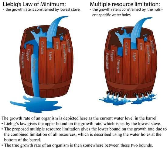
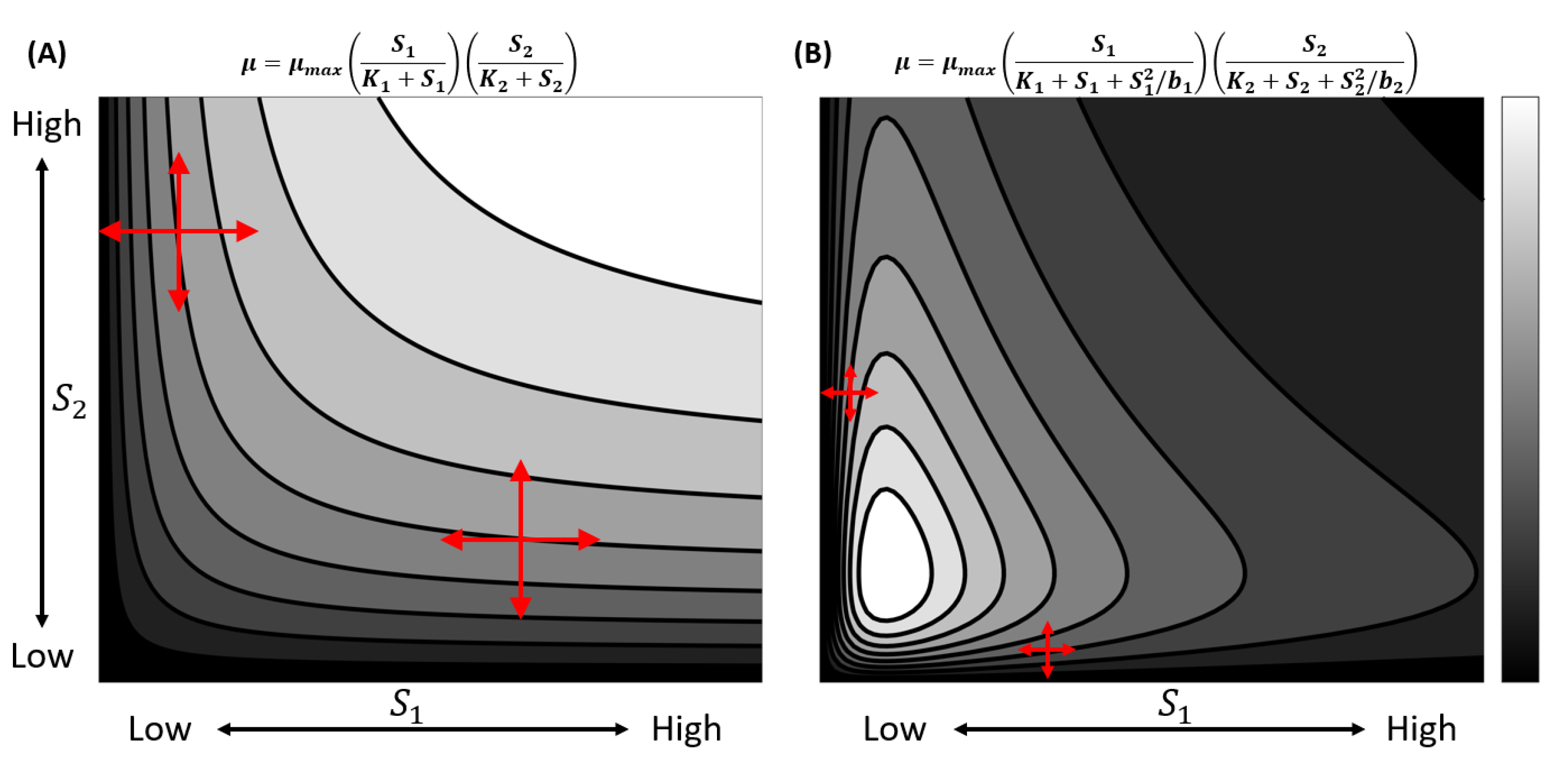
Liebig’s law of the minimum (LLM) posits that the growth rate of an organism is proportional to the supply of the single most limiting resource [1]. However, this may only be true locally and in limited cases [2]. It is more reasonable to consider each biological process within an organism to be determined by a specific set of resources. The overall growth of an organism is then the result of the interactions of all of these resources, or their combined limitation. Furthermore, due to the interconnected nature of these resources, changing the supply of one resource may have a cascading effect on the acquisition and processing of other resources [3,4]. Recent studies have reconciled LLM to be a special case within the complex growth dynamics plane [5,6,7,8]. Figure 1 shows two examples where LLM holds only along the contour curves that are parallel to a particular resource within the complex growth dynamic plane.

Existing frameworks for multiple resource limitation (MRL) often use multiplicative formulations (biochemical interactions) or threshold approaches based on the Droop cell quota growth formulation [5,7,8,9]. Some have studied the biochemical constraints that one resource has on another [6], while others have looked at the heterogeneity of resource limitation in the context of the producer–grazer (or predator–prey) [10,11,12,13]. Biochemical interactions of resources can explain the net result of multiple resource limitations, but MRL is likely more complicated due to the diversity of biochemical processes within an organism [14]. For example, it has been demonstrated that E. coli uses different resource allocation strategies to maintain the same growth rate under various resource limitations [15,16,17]. Others have also shown that plant–virus dynamics are altered under different resource treatments [18,19,20,21]. Growth functions that depend on biochemical constraints often ignore most aspects of the molecular mechanisms for growth, for example, they only consider the available supplies of each resource in proportion to the others. Thus, such functions would not be able to explain the mechanisms behind various growth strategies that arise in response to changes in growth conditions. On the other hand, it is straightforward to incorporate the constraints of growth machinery into threshold growth models [10,12]. However, while multiple resources are modeled in threshold models, growth is explicitly limited by a single resource at any given time. Thus, a gap exists between these two types of model formulations for multiple resource limitation (MRL).

In this study, we formulate a multiple resource limitation version of a previous threshold-type stoichiometric extension of the Lotka–Volterra model [10,11,12,13]. By considering the process of protein translation (an essential process driving growth), we also build a resource-explicit biomass conversion term. The new growth formulation retains key dynamical characteristics, especially at very high or low resource supplies, but also exhibits some unique characteristics. This model provides a description of growth based on multiple resource limitation and accounts for important aspects of the machinery that drives growth. As the threshold formulations of growth limitation often hinder global analysis, we hope that the smoothness of the new model may facilitate global analysis to uncover underlying biological properties and implications [22,23,24,25].

2. Methods

2.1. Formulation of the Multiple Resource Limitation

We first postulate that growth rates can depend on multiple resources. To present our thoughts on growth rate as a function of multiple limiting resources, we recall that Droop’s growth [26,27] rate equation takes the form of

$$\mu ={\mu }_{max}\left(1-\frac{q}{Q}\right).$$

(1)

Here, Q is the internal cell quota of the most growth-limiting resource (nmol cell ${}^{-1}$); q is the minimum or subsistence quota of the limiting resource at which the growth rate is zero; and ${\mu }_{max}$ is the theoretical maximum per capita population growth rate when all resources are abundant. Previous studies have also looked at possible mechanistic derivations of the Droop growth [28]. In the following, we shall formulate the co-limitation of multiple resources using nitrogen (N) and phosphorus (P) as an example due to their relevance in cell growth; however, the framework is also applicable to other resources, for example, the supply of light.

Since cells are made of proteins that are rich in N and protein production requires ribosomes that are rich in P, cell growth rates are functions of cellular N and P quotas. In the following, we assume $q_N$ and $q_P$ are the subsistence quota for N or P, respectively, while $Q_N$ and $Q_P$ are cellular N and P quotas, respectively. In reality, both N and P can be simultaneously limiting. According to LLM, cell growth rates take the form of

$${\mu }_l=min\{{\mu }_N,{\mu }_P\}={\mu }_{max}min\left\{\left(1-\frac{q_N}{Q_N}\right),\left(1-\frac{q_P}{Q_P}\right)\right\},$$

(2)

where ${\mu }_N$ and ${\mu }_P$ are the Droop growth function under the N and P limitation, respectively. Intuitively, since the production of ribosomes requires both N and P at the same time (e.g., ribosomes comprise both ribosomal proteins and RNA), while the production of non-ribosomal proteins does not involve P, one can argue that the protein production speed will be slower when both are in short supply, since it is highly dependent on the allocation of N in the translation phase. Hence, the true cell growth rate will be less, or at most, equal to ${\mu }_l$.

There are two possible extreme scenarios: (1) The cell takes up and uses N and P simultaneously; or (2) the cell takes up and uses N and P independently and sequentially. A real cell is likely to fall somewhere in between these two extreme scenarios, where there may be multiple factories that contribute to growth, but they all take up and process N and P at different rates. In case (1), the cell resource uptake process probably takes the least amount of time, and the cell growth rate may indeed take the form of ${\mu }_L$ assuming other resources may be sufficient for the growth process. In case (2), the resource uptake process probably takes the longest time, which may yield the slowest growth rate. Assume that the time to take up and use N is $T_N$, and the time to take up and use P is $T_P$. If P is abundant, then the cell’s N-limited growth rate is ${\mu }_N=1/T_N$. Likewise, the cell’s P-limited growth rate is ${\mu }_P=1/T_P$ when N is abundant. In case (2), the cell division time can be approximated by $T=T_N+T_P$, which implies that a plausible lower bound for the cell growth rate is approximately:

$${\mu }_m=\frac{1}{T}=\frac{1}{T_N+T_P}=\frac{1}{\frac{1}{{\mu }_N}+\frac{1}{{\mu }_P}}=\frac{{\mu }_N{\mu }_P}{{\mu }_N+{\mu }_P}.$$

(3)

We obtain the following theoretical bounds on growth rate $\mu$ under limitations by N and P:

$${\mu }_m<\mu <{\mu }_l.$$

(4)

If ${\mu }_N$ is much larger than ${\mu }_P$ (or the other way around), then the difference between ${\mu }_m$ and ${\mu }_l$ is much smaller, which gives a tighter range for the true growth rate $\mu$. For more specific considerations of co-limitation by N and P, we refer the readers to previous studies [29,30,31].

The theoretical forms of the multiple resource limitation and Liebig’s law of the minimum resemble two extreme instances of a production chain. Think of Liebig’s law in case (1) as a single large factory that takes in N and P and processes them simultaneously to make parts of a product (the NP-factory). In this case, there is no order for the processing of N or P. Once the relative numbers of the N-part and P-part are produced, they are then combined to make the final product. Thus, in this scenario, the rate that a complete product is produced is limited by the rate of the slower sub-production chain. On the other hand, the proposed multiple resource limitation in case (2) would be akin to two smaller factories in a production chain, where one exclusively handles N (the N-factory) to make product parts out of N, and moves these N-parts to the P-exclusive factory (the P-factory). The P-factory, then builds on these N-parts with P-parts to complete the process. Of course, the order may be reversed, but the key difference is that there is a strict order of operation in the second case. Thus, in this scenario, the uptake and processing times of N and P would then be additive, so the growth is much slower than the simultaneous process in case (1). Figure 2 describes this analogy. We remark that it is possible to formulate the growth equations for Liebig’s law of the minimum and the proposed multiple resource limitation based on these analogies.

A straightforward extension of this approach can yield a (lower) growth rate expression under MRL with more than two complementary limiting resources. Assume a cell grows under limitation by n resources $N_i$, $i=1,2\dots ,n$, and the time to take up and use resource $N_i$ is $T_i$. Then, the growth rate with only an i-th limiting resource is ${\mu }_i=1/T_i$. As in case (1) and case (2), we have

$${\mu }_L=min\{{\mu }_i:i=1,2,\dots n\},$$

(5)

and $T=T_1+T_2+\dots +T_n$, which implies that a plausible lower bound for the cell growth rate is approximately

$${\mu }_M=\frac{1}{T}=\frac{1}{T_1+T_2+\dots +T_n}=\frac{1}{\frac{1}{{\mu }_1}+\dots +\frac{1}{{\mu }_n}}$$

(6)

We thus arrive at the following theoretical bounds on growth rate $\mu$ under the limitations of multiple complementary resources:

$${\mu }_M<\mu <{\mu }_L.$$

(7)

Note that Equation (7) is the generalized version of Equation (4). This constraint is depicted in Figure 3. The graphical abstract depicts ${\mu }_M$ using the effects of the water holes and ${\mu }_L$ by the effect of the shortest stave. We also observe that as more limiting resources are considered, the region bounding the true growth (shaded green) expands solely due to the decrease in the lower bound ${\mu }_M$. This is expected, as the MRL formulation accounts for the contributions of additional limitations, which contrasts with Liebig’s formulation of growth. Furthermore, as one resource becomes more limiting (or the shorter the shortest stave of the barrel), the difference between ${\mu }_M$ and ${\mu }_L$ becomes smaller (Figure 3B).

Using this approach, we can replace Liebig’s growth law in the grazer (predator) equation of the LKE model [10] to obtain a new stoichiometric model with a smooth growth function.

2.2. Producer–Grazer Model Formulation

To formulate the producer–grazer model based on the MRL approach introduced here, we first state three main assumptions, which were used in the formulation of the LKE model [10]:

• The producer–grazer system is closed. This means the total amounts of phosphorus and carbon are conserved at all times. Furthermore, P and C are present either in the grazer or in the producer (i.e., there are no free pools of P or C).
• The minimum P:C ratio for the producer is q.
• The P:C ratio of the grazer is fixed at $\theta$.
• The grazer dies at a constant rate, d.

The model also has a set of assumptions distinct from the LKE model formulation:

5.

Intake phosphorus $P_{IN}$ can be partitioned into multiple parts for different purposes [17].

6.

The density of the producer is limited by light at a maximum K due to self-shading [10].

7.

The energy conversion efficiency for the grazer is an increasing function of the C:P ratio in the producer.

The densities of the producer and grazer are denoted by x and y, respectively, and are measured in terms of carbon in units of [mg C] [L ${}^{-1}$]. The dynamical system can be expressed in words as:

$$\begin{array}{cc}\hfill \left(\mathrm{Producer}\mathrm{rate}\mathrm{of}\mathrm{change}\right)& =\left(\mathrm{Growth}\mathrm{rate}\right)-\left(\mathrm{Predation}\mathrm{rate}\right)\hfill \\ \hfill \left(\mathrm{grazer}\mathrm{rate}\mathrm{of}\mathrm{change}\right)& =\left(\mathrm{Conversion}\mathrm{to}\mathrm{biomass}\right)\times \left(\mathrm{Predation}\mathrm{rate}\right)-\left(\mathrm{Death}\mathrm{rate}\right).\hfill \end{array}$$

By Assumption (4), we have

$$\left(\mathrm{Death}\mathrm{rate}\right)=dy.$$

(8)

Next, we represent the predation rate as a function of the producer x, specifically:

$$\left(\mathrm{Predation}\mathrm{rate}\right)=f\left(x\right)y.$$

(9)

Predation supplies both phosphorus and carbon for the grazer. In order to determine the amount of phosphorus intake per $f\left(x\right)y$, we first need to find the amount of phosphorus per x. We note that P: C is fixed at $\theta$ for the grazer, whose mass/density is given in terms of carbon, so $\theta y$ is the total amount of phosphorus in the grazer population at any given time. Since the total amount of phosphorus (P) is conserved in the system, the total amount of phosphorus in the producer population is given by $(P-\theta y)$. Then, the P:C ratio for the producer is $Q=(P-\theta y)/x$. Thus, the total amount of phosphorus acquired from predation is $Q\times f\left(x\right)y$.

However, not all of the acquired phosphorus is used for biomass production. Some are used to maintain and build cellular machinery that produces new biomass [32,33]. Assumption (5) allows us to partition the intake phosphorus $P_{IN}$ into two parts: $P_R$ and $P_P$. $P_R$ is the amount of phosphorus that goes into maintaining the existing machinery. On the other hand, $P_P$ is the phosphorus reserved to be used for biomass synthesized by $P_R$ (i.e., growth). We consider an optimal proportional function $\alpha (·)$, which optimizes the growth process by optimizing the fraction of phosphorus that goes into $P_P$ and $P_R$. In other words, the most efficient division would have each $P_R$ process the $\alpha (·)$ unit of $P_P$ per unit of time to build biomass. The $\alpha (·)$ relates to the biomass production efficiency; for example, if $\alpha (·)$ is much less than 1, then there is very low efficiency—almost all the P intake goes into maintaining the machinery. On the other hand, if $\alpha (·)$ is large, then most of the P intake goes into making new biomass. Together, we have

$$P_{IN}=P_R+P_P=P_R+\alpha (·)P_R=\left(1+\alpha (·)\right)P_R.$$

(10)

Solving for $P_R$ and $P_P$, we get:

$$P_R=\frac{1}{1+\alpha (·)}{P}_{IN}\mathrm{and}{P}_P=\frac{\alpha (·)}{1+\alpha (·)}{P}_{IN}.$$

(11)

Since the only source of phosphorus acquisition for the grazer in this model is through predation, $P_{IN}=Q\times f\left(x\right)y$. Thus, the rate of phosphorus being used for the synthesis of biomass is:

$$P_P=\frac{\alpha (·)}{1+\alpha (·)}{P}_{IN}=\frac{\alpha (·)}{1+\alpha (·)}Qf\left(x\right)y.$$

(12)

However, note that the biomass synthesis must be in terms of carbon (since units of x and y are given in terms of carbon). This means we need to convert P biomass production to carbon. Since we know that P:C is fixed at $\theta$ for the grazer, the biomass acquired from hunting in terms of carbon is:

$$\left(\mathrm{Conversion}\mathrm{to}\mathrm{biomass}\right)\times \left(\mathrm{Predation}\mathrm{rate}\right)=\left(\frac{1}{\theta }\frac{\alpha (·)}{1+\alpha (·)}\right)\left(Qf\left(x\right)y\right)=\frac{\alpha (·)}{1+\alpha (·)}\frac{Qf\left(x\right)y}{\theta }.$$

(13)

Together, the rate of change equation for the grazer is:

$$\frac{dy}{dt}=\frac{\alpha (·)}{1+\alpha (·)}\frac{Qf\left(x\right)y}{\theta }-dy.$$

(14)

Next, we look at the growth rate of x. By Assumption (6), we can use the Droop formulation for the growth rate of x, so its growth assumes the carbon limitation:

$$\mu \left(1-\frac{x}{K}\right).$$

(15)

Additionally, producer growth can be limited by phosphorus supply. Since the minimum P:C ratio for the producer is q, we have a second upper limit on producer density (in terms of carbon) of $(P-\theta y)/q$. This gives an expression for growth limited by phosphorus as:

$$\mu \left(1-\frac{x}{(P-\theta y)/q}\right)=\mu \left(1-\frac{q}{Q}\right).$$

(16)

Using the proposed co-limitation form of growth in Equation (6) in Section 2.1, the growth of the producer is given by:

$$\mu \frac{\left(1-\frac{x}{K}\right)\left(1-\frac{q}{Q}\right)}{\left(1-\frac{x}{K}\right)+\left(1-\frac{q}{Q}\right)}$$

(17)

In the overall growth under MRL, the net growth is assumed to be modulated by the Droop formula relative to each resource. At infinite resource ($K\to \infty ,Q\to \infty$), the net growth under the proposed MRL formulation converges to half of the absolute maximum growth $\mu$. Together with Equation (14), we obtain the governing equations for the producer–grazer dynamics:

$$\begin{array}{cc}\hfill \frac{dx}{dt}& =\mu \frac{\left(1-\frac{x}{K}\right)\left(1-\frac{q}{Q}\right)}{\left(1-\frac{x}{K}\right)+\left(1-\frac{q}{Q}\right)}x-f\left(x\right)y\hfill \end{array}$$

(18)

$$\begin{array}{cc}\hfill \frac{dy}{dt}& =\frac{\alpha (·)}{1+\alpha (·)}\frac{Qf\left(x\right)y}{\theta }-dy.\hfill \end{array}$$

(19)

We shall use the abbreviation MRL model to denote this new proposed model, which, in contrast to earlier stoichiometric formulation such as the LKE model [10,12], contains no minimum function. In the MRL model, the function $\alpha (·)$ incorporates the effects of energy conversion efficiency using C as a surrogate, as in the previous formulation [10]. By Assumption (7), we take $\alpha (·)$ to be an increasing function of $1/Q$ (or the C:P ratio). We use a saturation function to represent the functional form of $\alpha (·):$

$$\alpha \left(\frac{1}{Q}\right)=a\frac{(1/Q)}{m+(1/Q)}=\frac{a}{mQ+1}.$$

(20)

Here, a is the maximum efficiency of biomass production (which is based on the amount of phosphorus partitioned into biomass production). The m is the half-saturation of biomass production efficiency. This saturation form of $\alpha (·)$ gives:

$$\frac{\alpha (·)}{1+\alpha (·)}=\frac{a}{a+mQ+1}.$$

(21)

Finally, for the predation functional response $f\left(x\right)$, we choose a Monod-type function [10].

$$f\left(x\right)=\frac{cx}{k+x},$$

(22)

where c and k are the maximum ingestion rate of the grazer and the half-saturation of the grazer ingestion response, respectively. We will compare the MRL model with the threshold formulation LKE model [10].

$$\begin{array}{cc}\hfill \frac{dx}{dt}& =\mu x\left(1-\frac{x}{min\left(K,(P-\theta y)/q\right)}\right)-f\left(x\right)y\hfill \end{array}$$

(23)

$$\begin{array}{cc}\hfill \frac{dy}{dt}& =b_{1}min\left(1,\frac{(P-\theta y)/x}{\theta }\right)f\left(x\right)y-dy.\hfill \end{array}$$

(24)

Here, $b_1$ is the efficiency conversion rate for energy (C).

2.3. The LKE and the MRL Models

In summary, the LKE model takes the form:

$$\begin{array}{cc}\hfill \frac{dx}{dt}& =\mu x\left(1-\frac{x}{min\left(K,(P-\theta y)/q\right)}\right)-\frac{cx}{k+x}y\hfill \end{array}$$

(25)

$$\begin{array}{cc}\hfill \frac{dy}{dt}& =b_{1}min\left(1,\frac{(P-\theta y)/x}{\theta }\right)\frac{cx}{k+x}y-dy.\hfill \end{array}$$

(26)

The MRL model takes on the following form for comparison purposes:

$$\begin{array}{cc}\hfill \frac{dx}{dt}& =\mu \frac{\left(1-\frac{x}{K}\right)\left(1-\frac{q}{Q}\right)}{\left(1-\frac{x}{K}\right)+\left(1-\frac{q}{Q}\right)}x-\frac{cx}{k+x}y\hfill \end{array}$$

(27)

$$\begin{array}{cc}\hfill \frac{dy}{dt}& =\frac{a}{a+mQ+1}\frac{cx}{k+x}\frac{Q}{\theta }y-dy.\hfill \end{array}$$

(28)

3. Results

3.1. Basic Biological Properties

We consider several basic biological properties of the proposed model in Equations (18) and (19), and the extension model in Equations (27) and (28). These properties are summarized in Theorem 1. This theorem guarantees the positivity and boundedness of the solution to the system given by Equations (18) and (19), and is a consequence of the biological assumptions in the model formulation.

Theorem 1.

The biological solutions to the system given by Equations (18) and (19) are eventually bounded within the set$\Omega =\left\{(x,y):x,y>0,x\le min\{K,P/q\},y\le P/\theta \right\}$.

To understand why this theorem is true, let us consider the biological assumption of the closed system represented by Equations (18) and (19). For positivity, note that the rates of change for the producer and grazer are proportional to their biomass, so their biomass cannot become negative (otherwise, it would lead to a contradiction). For the upper bound, since the system has a fixed amount of phosphorus P and the producer has a minimum cell quota of q, the producer biomass cannot exceed $P/q$. If the producer biomass exceeds $P/q$, its growth term immediately becomes negative, which results in an overall negative rate of change. The producer biomass is also limited by light (K). Thus, together, the producer biomass cannot exceed $min\{K,P/q\}$. In the case of the grazer, the fixed amount of phosphorus in the system and a fixed P:C ratio $\theta$ imply that its biomass is limited by $P/\theta$. Thus, the set $\Omega$ denotes the biological region of the system. Solutions outside of this region exist, but are not biologically relevant.

3.2. Model Simulation and Comparison

Table 1. Baseline parameter values taken from [10,12]. a and m were chosen so that $\alpha (·)$ gives values in the proximity of $b_1$ (note that $\alpha (·)$ varies with the model dynamics).

Parameter		Value	Unit
P	Total phosphorus	0.025	mg P L ${}^{-1}$
$\mu$	Overall maximal growth rate	1.2	day ${}^{-1}$
K	Producer carrying capacity (light limited)	0.5	mg C L ${}^{-1}$
q	Producer minimal P/C	0.0038	(mg P)/(mg C)
$\theta$	grazer constant P/C	0.03	(mg P)/(mg C)
$b_1$	Theoretical maximum efficiency of biomass production	0.8
a	Maximum efficiency of biomass production (energy)	8
m	Half-saturation of biomass production efficiency	200	(mg C)/(mg P)
c	Maximum ingestion rate of the grazer	0.81	day${}^{-1}$
k	Half-saturation of grazer ingestion response	0.25	mg C L ${}^{-1}$
d	Grazer loss rate	0.25	day ${}^{-1}$

summarizes the baseline parameter values used for the simulation results. While most parameters have been taken from previous studies [10,12]. a and m were chosen so that $\alpha (·)$ gives a similar value to $b_1$. Note that the maximum conversion efficiency for energy (as indexed by C) must be less than 1 due to the second law of thermodynamics. However, in theory, the maximum conversion efficiency for a limiting resource such as P or N can be 1, if the organism can physiologically sequester all resources it obtains from its food or environment.

Loladze and colleagues demonstrated that the LKE model contains “a paradox of energy enrichment”, where energy enrichment (increasing the light-limited carrying capacity K) decreases the grazer density (and, indeed, can cause grazer extinction) by lowering food quality, an important contribution to the theory of predator–prey by highlighting the impacts of food quality. Later models built on the same framework also show similar qualitative properties, which led to the impression that the paradox of energy is unique to the threshold (minimum) formulations in the LKE model [12,22]. Here we show that the MRL model, with its distinct formulation without minimum terms, retains this key feature of the LKE model. Specifically, increasing K results in the deterministic extinction of the grazer in the MRL model, see Figure 4. Furthermore, as expected from the model formulation, the MRL model gives a lower bound on the growth dynamics. For example, when $K=0.25$ mg C/L, the MRL model shows transient oscillations that persist for some time before dampening toward a steady-state with lower values than those seen in the LKE model. When $K=2$ mg C/L, the MRL model also shows a clear distinction in the speed of convergence to the steady-state value. For moderate K, the MRL model shows periodic solutions that are typical of predator–prey models [19,34,35,36]. However, the periodic behaviors in the MRL model seem to act on a slower time scale, creating long phases of slow increase/decrease in the density of the producer and grazer as compared to the LKE model. For example, when $K=0.75$, the oscillation period of the grazer population is about 40 days in the MRL model vs. 20 days in the LKE model. The simulation results in Figure 4 suggest that, due to slower growth dynamics, the MRL model is more susceptible to oscillations, including transient ones, compared to the LKE model. This hints at the possibility that the MRL model may be suitable for the study of periodic behaviors on long time-scales, and thus is relevant for certain biological systems, such as snowshoe hares [37].

Next, we turn our attention to the effect of resource limitation on model dynamics. Figure 5 shows the asymptotic behaviors of the MRL (A) and LKE (B) models with respect to resource limitation parameters K and P. The bifurcation plot confirms the paradox of energy enrichment observed in Figure 4. Furthermore, Elser et al. (2012) and Peace et al. (2013) discussed and formulated models to study a phenomenon known as the “stoichiometric knife-edge” in which excess food resource content (in addition to low food resource content) can lead to the collapse of the grazer population [11,12,22]. In previous studies, the stoichiometric knife edge effect was incorporated by capping the ingestion rate of phosphorus per each unit of the grazer’s biomass per time. Here, we propose to incorporate a mechanism for this observation via a trade-off in energy conversion efficiency using the function $\alpha (·)$. While the MRL model does not result in a deterministic extinction as P increases, the grazer population at high P oscillates dangerously close to 0, which increases the probability of a stochastic extinction event.

When comparing the asymptotic bifurcation of the MRL model to the LKE model as K varies, we find that the MRL model predicts a lower value of K at which extinction occurs ($K\approx 1.5$ vs. $K\approx 1.9$), and at which oscillatory behaviors arise ($K\approx 0.25$ vs. $K\approx 0.55$). Together, the oscillatory region in the MRL model is roughly twice as large as in the LKE model (0.9 vs. 0.45 unit of K). Additionally, as P increases, the LKE model predicts a saturation on the effect of P as K becomes the limiting resource ($P\approx 0.02$). This means the LKE model does not exhibit the stoichiometric knife-edge effect.

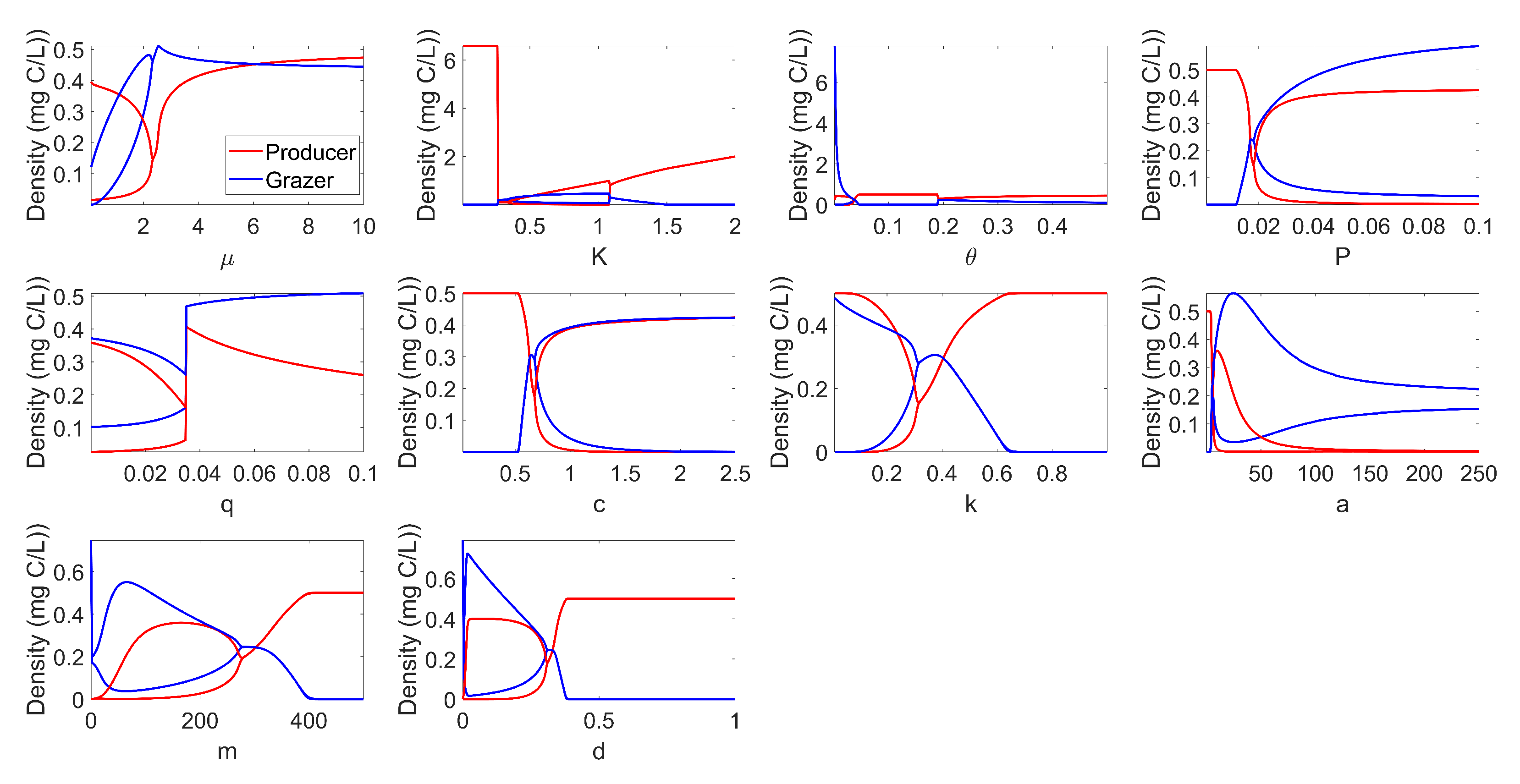
The complete bifurcation analysis of the system with respect to each model parameter is provided in Figure A1 in the Appendix A. Figure A1 demonstrates several interesting bifurcations for this model. First, we note that varying a number of parameters can lead towards or away from a stable periodic solution (Hopf bifurcation). Furthermore, for very low values of K, we see that the solution of the system converges to a very high producer-only equilibrium. While this boundary equilibrium is of mathematical interest, it is not within the biologically relevant region $\Omega$ in Theorem 1.

4. Discussion

The growth of an organism is a complex process governed by trade-offs between the maintenance and operation of various biochemical processes relative to environmental factors [38,39,40,41]. Understanding the interactive network of factors that determines the growth of an organism and its manifestations on a population scale has been of interest to the wider scientific community for a long time, due to many practical applications and the potential to gain insights into fundamental biological processes [42,43,44,45,46,47,48,49,50]. In particular, incorporation of growth laws into predator–prey systems is necessary to explain a range of non-intuitive experimental observations, such as the paradox of energy enrichment, which cannot be explained with the classic Lotka–Volterra model [10,11,12,51].

The proposed multiple resource limitation enforces a lower bound on growth dynamics. Previous threshold models of growth with multiple resources using the minimum function are intrinsically single-resource limited; that is, both resources do not limit growth simultaneously. In order to explicitly incorporate the potential for the interactive effects of multiple resources on the growth of an organism simultaneously, we assume that each resource is taken up and processed independently of other resources. Doing so provides a lower bound on the net processing rate of all resources, giving a lower bound on the growth rate. This contrasts with the symmetric functional growth forms of multiple resource limitations in the literature, which are often built based on Monod growth kinetics. As a consequence of this assumption, our theoretical and numerical simulations show that the proposed model exhibits slower growth dynamics and is more susceptible to oscillatory behavior. We also demonstrated that the proposed model is able to capture a wide range of experimental observations, such as the paradox of enrichment, the paradox of energy enrichment, and the paradox of nutrient enrichment (see the bifurcation with respect to K and P in Figure 5A). Furthermore, we provided a possible mechanism based on resource allocation and energy conversion efficiency to explain why increasing P can result in the collapse of the grazer’s population.

A shift in the paradigm of modeling growth dynamics. In modeling studies, researchers often attempt to find the best model fit to the growth data of an organism. However, the precise growth function is never known, leading to potential issues of interpretation and prediction for the dynamics of the system. Instead, we suggest using upper and lower bounds on growth to constrain possible dynamics of the system. For example, one can use both Liebig’s law of the minimum and the proposed MRL models to look at possible dynamical behaviors of a biological system. Figure 4 shows an example of this approach. Here, the possible dynamical behaviors of the system are expected to fall somewhere between the predicted dynamics of the two models. Thus, instead of trying to match an arbitrary model to the growth data and using the uncertainty associated with the measurements to predict possible dynamical behaviors of the system, our proposed modeling approach does so by accounting for the uncertainty associated with the model formulation. This alternative approach can open new research revenues to develop more insights into the growth of different organisms under different conditions and their impact on the whole system.

Multiple resource limitations and further integration. The importance of multiple resource limitations has been highlighted in various studies, such as the effect of the interaction between resources, such as between N and P, on primary producer communities in various ecosystems [52,53,54,55], and even for essential micro- and macro-nutrients, such as amino acids, sterols, carbohydrates, proteins, and lipids [56,57,58]. Furthermore, the effect of each resource is not independent of others, and their interactive effect can alter how organisms respond to their environment and vice versa [59,60,61,62,63,64,65]. This further supports the use of the multiple resource limitation frameworks. Our formulation of multiple resource limitations provides a lower bound on growth; however, it does not take on any specific functional form of growth. The example of its integration in the LKE model assumes a Droop growth form, but the formulation itself is not restricted to Droop growth. In fact, when considering the limitations of multiple resources with known interactions, suitable growth functions that account for their interactions can also be integrated similarly. Thus, it is possible to extend this approach to better understand complex data of multiple resource limitations, such as in the field of ionomics [66,67,68].

This formulation of a representative system with our proposed multiple resource limitation framework skims over a number of important biological factors, such as the time it takes for resources to be recycled, spatial components, and trait-based variation effects, among others [69,70]. These effects can be incorporated by considering models with a time-delay and spatial structure [71,72], or even pseudo-spatial models that use patches to imitate the spatial structure in populations [73]. We also only consider one producer (prey) and one grazer (predator) species in our integration of the MRL growth form. However, it is straightforward to incorporate the same MRL growth form to richer dynamical systems with multiple trophic levels or multiple species of producers and grazers in various settings (e.g., chemostats) [42,74,75,76,77,78]. Finally, these results suggest the possibility of using both models simultaneously to establish bounds on the growth of an organism. One could perhaps use growth data to test this hypothesis [76,79,80]. Future research can further develop these aspects of the proposed MRL framework and test it using experimental data to explain empirical observations, generalize empirical growth laws, and enhance our understanding of the growth dynamics in multi-species systems.

References

- Von Liebig, J. Die Organische Chemie in Ihrer Anwendung auf Agricultur und Physiologie; Taylor and Walton: London, UK, 1841. [Google Scholar]
- Gorban, A.N.; Pokidysheva, L.I.; Smirnova, E.V.; Tyukina, T.A. Law of the minimum paradoxes. Bull. Math. Biol. 2011, 73, 2013–2044. [Google Scholar] [CrossRef] [PubMed] [Green Version]
- Jeyasingh, P.D.; Sherman, R.E.; Prater, C.; Pulkkinen, K.; Ketola, T. Adaptation to a limiting element involves mitigation of multiple elemental imbalances. J. R. Soc. Interface 2023, 20, 20220472. [Google Scholar] [CrossRef] [PubMed]
- Williams, R.J.P.; Da Silva, J.F. The Chemistry of Evolution: The Development of Our Ecosystem; Elsevier: Amsterdam, The Netherlands, 2005. [Google Scholar]
- Saito, M.A.; Goepfert, T.J.; Ritt, J.T. Some thoughts on the concept of colimitation: Three definitions and the importance of bioavailability. Limnol. Oceanogr. 2008, 53, 276–290. [Google Scholar] [CrossRef] [Green Version]
- Pahlow, M.; Oschlies, A. Chain model of phytoplankton P, N and light colimitation. Mar. Ecol. Prog. Ser. 2009, 376, 69–83. [Google Scholar] [CrossRef]
- Sperfeld, E.; Martin-Creuzburg, D.; Wacker, A. Multiple resource limitation theory applied to herbivorous consumers: Liebig’s minimum rule vs. interactive co-limitation. Ecol. Lett. 2012, 15, 142–150. [Google Scholar] [CrossRef]
- Sperfeld, E.; Raubenheimer, D.; Wacker, A. Bridging factorial and gradient concepts of resource co-limitation: Towards a general framework applied to consumers. Ecol. Lett. 2016, 19, 201–215. [Google Scholar] [CrossRef] [Green Version]
- Cherif, M.; Loreau, M. Towards a more biologically realistic use of Droop’s equations to model growth under multiple nutrient limitation. Oikos 2010, 119, 897–907. [Google Scholar] [CrossRef]
- Loladze, I.; Kuang, Y.; Elser, J.J. Stoichiometry in producer–grazer systems: Linking energy flow with element cycling. Bull. Math. Biol. 2000, 62, 1137–1162. [Google Scholar] [CrossRef]
- Elser, J.J.; Loladze, I.; Peace, A.L.; Kuang, Y. Lotka re-loaded: Modeling trophic interactions under stoichiometric constraints. Ecol. Model. 2012, 245, 3–11. [Google Scholar] [CrossRef]
- Peace, A.; Zhao, Y.; Loladze, I.; Elser, J.J.; Kuang, Y. A stoichiometric producer–grazer model incorporating the effects of excess food-nutrient content on consumer dynamics. Math. Biosci. 2013, 244, 107–115. [Google Scholar] [CrossRef]
- Yamamichi, M.; Meunier, C.L.; Peace, A.; Prater, C.; Rúa, M.A. Rapid evolution of a consumer stoichiometric trait destabilizes consumer–producer dynamics. Oikos 2015, 124, 960–969. [Google Scholar] [CrossRef]
- Isanta-Navarro, J.; Prater, C.; Peoples, L.M.; Loladze, I.; Phan, T.; Jeyasingh, P.D.; Church, M.J.; Kuang, Y.; Elser, J.J. Revisiting the growth rate hypothesis: Towards a holistic stoichiometric understanding of growth. Ecol. Lett. 2022, 25, 2324–2339. [Google Scholar] [CrossRef]
- Li, S.H.J.; Li, Z.; Park, J.O.; King, C.G.; Rabinowitz, J.D.; Wingreen, N.S.; Gitai, Z. Escherichia coli translation strategies differ across carbon, nitrogen and phosphorus limitation conditions. Nat. Microbiol. 2018, 3, 939–947. [Google Scholar] [CrossRef]
- Iyer, S.; Le, D.; Park, B.R.; Kim, M. Distinct mechanisms coordinate transcription and translation under carbon and nitrogen starvation in Escherichia coli. Nat. Microbiol. 2018, 3, 741–748. [Google Scholar] [CrossRef]
- Phan, T.; He, C.; Loladze, I.; Prater, C.; Elser, J.; Kuang, Y. Dynamics and growth rate implications of ribosomes and mRNAs interaction in E. coli. Heliyon 2022, 8, e09820. [Google Scholar] [CrossRef]
- Borer, E.T.; Paseka, R.E.; Peace, A.; Asik, L.; Everett, R.; Frenken, T.; González, A.L.; Strauss, A.T.; Van de Waal, D.B.; White, L.A.; et al. Disease-mediated nutrient dynamics: Coupling host–pathogen interactions with ecosystem elements and energy. Ecol. Monogr. 2022, 92, e1510. [Google Scholar] [CrossRef]
- Phan, T.; Pell, B.; Kendig, A.E.; Borer, E.T.; Kuang, Y. Rich dynamics of a simple delay host-pathogen model of cell-to-cell infection for plant virus. Discret. Contin. Dyn. Syst. B 2021, 26, 515. [Google Scholar] [CrossRef]
- Kendig, A.E.; Borer, E.T.; Boak, E.N.; Picard, T.C.; Seabloom, E.W. Host nutrition mediates interactions between plant viruses, altering transmission and predicted disease spread. Ecology 2020, 101, e03155. [Google Scholar] [CrossRef]
- Pell, B.; Kendig, A.E.; Borer, E.T.; Kuang, Y. Modeling nutrient and disease dynamics in a plant-pathogen system. Math. Biosci. Eng. 2019, 16, 234–264. [Google Scholar] [CrossRef]
- Peace, A.; Wang, H.; Kuang, Y. Dynamics of a producer–grazer model incorporating the effects of excess food nutrient content on grazer’s growth. Bull. Math. Biol. 2014, 76, 2175–2197. [Google Scholar] [CrossRef]
- Kong, J.D.; Salceanu, P.; Wang, H. A stoichiometric organic matter decomposition model in a chemostat culture. J. Math. Biol. 2018, 76, 609–644. [Google Scholar] [CrossRef] [PubMed]
- Peace, A.; Wang, H. Compensatory foraging in stoichiometric producer–grazer models. Bull. Math. Biol. 2019, 81, 4932–4950. [Google Scholar] [CrossRef] [PubMed]
- Ji, J.; Wang, H. Competitive Exclusion and Coexistence in a Stoichiometric Chemostat Model. J. Dyn. Differ. Equ. 2022, 1–33. [Google Scholar] [CrossRef]
- Droop, M. The nutrient status of algal cells in continuous culture. J. Mar. Biol. Assoc. UK 1974, 54, 825–855. [Google Scholar] [CrossRef]
- Wang, H.; Garcia, P.V.; Ahmed, S.; Heggerud, C.M. Mathematical comparison and empirical review of the Monod and Droop forms for resource-based population dynamics. Ecol. Model. 2022, 466, 109887. [Google Scholar] [CrossRef]
- Pahlow, M.; Oschlies, A. Optimal allocation backs Droop’s cell-quota model. Mar. Ecol. Prog. Ser. 2013, 473, 1–5. [Google Scholar] [CrossRef] [Green Version]
- Loladze, I. Iterative chemostat: A modelling framework linking biosynthesis to nutrient cycling on ecological and evolutionary time scales. Math. Biosci. Eng. 2019, 16, 990–1004. [Google Scholar] [CrossRef]
- Loladze, I.; Elser, J.J. The origins of the Redfield nitrogen-to-phosphorus ratio are in a homoeostatic protein-to-rRNA ratio. Ecol. Lett. 2011, 14, 244–250. [Google Scholar] [CrossRef]
- Kafri, M.; Metzl-Raz, E.; Jonas, F.; Barkai, N. Rethinking cell growth models. FEMS Yeast Res. 2016, 16, fow081. [Google Scholar] [CrossRef] [Green Version]
- Sterner, R.W.; Elser, J.J. Ecological stoichiometry. In Ecological Stoichiometry; Princeton University Press: Princeton, NJ, USA, 2017. [Google Scholar]
- Scott, M.; Gunderson, C.W.; Mateescu, E.M.; Zhang, Z.; Hwa, T. Interdependence of cell growth and gene expression: Origins and consequences. Science 2010, 330, 1099–1102. [Google Scholar] [CrossRef]
- Hsu, S.B.; Hwang, T.W.; Kuang, Y. Global analysis of the Michaelis–Menten-type ratio-dependent predator–prey system. J. Math. Biol. 2001, 42, 489–506. [Google Scholar] [CrossRef] [PubMed]
- Gourley, S.A.; Kuang, Y. A stage structured predator–prey model and its dependence on maturation delay and death rate. J. Math. Biol. 2004, 49, 188–200. [Google Scholar] [CrossRef] [PubMed]
- Dai, Y.; Zhao, Y.; Sang, B. Four limit cycles in a predator–prey system of Leslie type with generalized Holling type III functional response. Nonlinear Anal. Real World Appl. 2019, 50, 218–239. [Google Scholar] [CrossRef] [Green Version]
- Wang, H.; Nagy, J.D.; Gilg, O.; Kuang, Y. The roles of predator maturation delay and functional response in determining the periodicity of predator–prey cycles. Math. Biosci. 2009, 221, 1–10. [Google Scholar] [CrossRef]
- Wu, C.; Balakrishnan, R.; Braniff, N.; Mori, M.; Manzanarez, G.; Zhang, Z.; Hwa, T. Cellular perception of growth rate and the mechanistic origin of bacterial growth law. Proc. Natl. Acad. Sci. USA 2022, 119, e2201585119. [Google Scholar] [CrossRef]
- Li, Z.; Liu, B.; Li, S.H.J.; King, C.G.; Gitai, Z.; Wingreen, N.S. Modeling microbial metabolic trade-offs in a chemostat. PLoS Comput. Biol. 2020, 16, e1008156. [Google Scholar] [CrossRef]
- Basan, M.; Honda, T.; Christodoulou, D.; Hörl, M.; Chang, Y.F.; Leoncini, E.; Mukherjee, A.; Okano, H.; Taylor, B.R.; Silverman, J.M.; et al. A universal trade-off between growth and lag in fluctuating environments. Nature 2020, 584, 470–474. [Google Scholar] [CrossRef]
- Guignard, M.S.; Leitch, A.R.; Acquisti, C.; Eizaguirre, C.; Elser, J.J.; Hessen, D.O.; Jeyasingh, P.D.; Neiman, M.; Richardson, A.E.; Soltis, P.S.; et al. Impacts of nitrogen and phosphorus: From genomes to natural ecosystems and agriculture. Front. Ecol. Evol. 2017, 5, 70. [Google Scholar] [CrossRef] [Green Version]
- Klausmeier, C.A.; Litchman, E.; Levin, S.A. Phytoplankton growth and stoichiometry under multiple nutrient limitation. Limnol. Oceanogr. 2004, 49, 1463–1470. [Google Scholar] [CrossRef] [Green Version]
- Packer, A.; Li, Y.; Andersen, T.; Hu, Q.; Kuang, Y.; Sommerfeld, M. Growth and neutral lipid synthesis in green microalgae: A mathematical model. Bioresour. Technol. 2011, 102, 111–117. [Google Scholar] [CrossRef]
- Loladze, I. Hidden shift of the ionome of plants exposed to elevated CO2 depletes minerals at the base of human nutrition. eLife 2014, 3, e02245. [Google Scholar] [CrossRef]
- Marquet, P.A.; Allen, A.P.; Brown, J.H.; Dunne, J.A.; Enquist, B.J.; Gillooly, J.F.; Gowaty, P.A.; Green, J.L.; Harte, J.; Hubbell, S.P.; et al. On theory in ecology. BioScience 2014, 64, 701–710. [Google Scholar] [CrossRef] [Green Version]
- Zhu, C.; Kobayashi, K.; Loladze, I.; Zhu, J.; Jiang, Q.; Xu, X.; Liu, G.; Seneweera, S.; Ebi, K.L.; Drewnowski, A.; et al. Carbon dioxide (CO2) levels this century will alter the protein, micronutrients, and vitamin content of rice grains with potential health consequences for the poorest rice-dependent countries. Sci. Adv. 2018, 4, eaaq1012. [Google Scholar] [CrossRef] [Green Version]
- Curtsdotter, A.; Banks, H.T.; Banks, J.E.; Jonsson, M.; Jonsson, T.; Laubmeier, A.N.; Traugott, M.; Bommarco, R. Ecosystem function in predator–prey food webs—Confronting dynamic models with empirical data. J. Anim. Ecol. 2019, 88, 196–210. [Google Scholar] [CrossRef] [Green Version]
- Heggerud, C.M.; Wang, H.; Lewis, M.A. Transient dynamics of a stoichiometric cyanobacteria model via multiple-scale analysis. SIAM J. Appl. Math. 2020, 80, 1223–1246. [Google Scholar] [CrossRef]
- Peace, A.; Frost, P.C.; Wagner, N.D.; Danger, M.; Accolla, C.; Antczak, P.; Brooks, B.W.; Costello, D.M.; Everett, R.A.; Flores, K.B.; et al. Stoichiometric ecotoxicology for a multisubstance world. BioScience 2021, 71, 132–147. [Google Scholar] [CrossRef]
- Feng, Z.; DeAngelis, D.L. Mathematical Models of Plant-Herbivore Interactions; Chapman and Hall/CRC: Boca Raton, FL, USA, 2017. [Google Scholar]
- Peace, A.; Poteat, M.D.; Wang, H. Somatic growth dilution of a toxicant in a predator–prey model under stoichiometric constraints. J. Theor. Biol. 2016, 407, 198–211. [Google Scholar] [CrossRef] [Green Version]
- Elser, J.J.; Bracken, M.E.; Cleland, E.E.; Gruner, D.S.; Harpole, W.S.; Hillebrand, H.; Ngai, J.T.; Seabloom, E.W.; Shurin, J.B.; Smith, J.E. Global analysis of nitrogen and phosphorus limitation of primary producers in freshwater, marine and terrestrial ecosystems. Ecol. Lett. 2007, 10, 1135–1142. [Google Scholar] [CrossRef] [Green Version]
- Allgeier, J.E.; Rosemond, A.D.; Layman, C.A. The frequency and magnitude of non-additive responses to multiple nutrient enrichment. J. Appl. Ecol. 2011, 48, 96–101. [Google Scholar] [CrossRef]
- Harpole, W.S.; Ngai, J.T.; Cleland, E.E.; Seabloom, E.W.; Borer, E.T.; Bracken, M.E.; Elser, J.J.; Gruner, D.S.; Hillebrand, H.; Shurin, J.B.; et al. Nutrient co-limitation of primary producer communities. Ecol. Lett. 2011, 14, 852–862. [Google Scholar] [CrossRef]
- Prater, C.; Bullard, J.E.; Osburn, C.L.; Martin, S.L.; Watts, M.J.; Anderson, N.J. Landscape controls on nutrient stoichiometry regulate lake primary production at the margin of the Greenland Ice Sheet. Ecosystems 2022, 25, 931–947. [Google Scholar] [CrossRef]
- Lee, K.P.; Simpson, S.J.; Clissold, F.J.; Brooks, R.; Ballard, J.W.O.; Taylor, P.W.; Soran, N.; Raubenheimer, D. Lifespan and reproduction in Drosophila: New insights from nutritional geometry. Proc. Natl. Acad. Sci. USA 2008, 105, 2498–2503. [Google Scholar] [CrossRef] [PubMed] [Green Version]
- Jensen, K.; Mayntz, D.; Toft, S.; Clissold, F.J.; Hunt, J.; Raubenheimer, D.; Simpson, S.J. Optimal foraging for specific nutrients in predatory beetles. Proc. R. Soc. B Biol. Sci. 2012, 279, 2212–2218. [Google Scholar] [CrossRef] [PubMed] [Green Version]
- Wacker, A.; Martin-Creuzburg, D. Biochemical nutrient requirements of the rotifer B rachionus calyciflorus: Co-limitation by sterols and amino acids. Funct. Ecol. 2012, 26, 1135–1143. [Google Scholar] [CrossRef] [Green Version]
- Elser, J.J.; Peace, A.L.; Kyle, M.; Wojewodzic, M.; McCrackin, M.L.; Andersen, T.; Hessen, D.O. Atmospheric nitrogen deposition is associated with elevated phosphorus limitation of lake zooplankton. Ecol. Lett. 2010, 13, 1256–1261. [Google Scholar] [CrossRef]
- Prater, C.; Wagner, N.D.; Frost, P.C. Effects of calcium and phosphorus limitation on the nutritional ecophysiology of D aphnia. Limnol. Oceanogr. 2016, 61, 268–278. [Google Scholar] [CrossRef] [Green Version]
- Halvorson, H.M.; Sperfeld, E.; Evans-White, M.A. Quantity and quality limit detritivore growth: Mechanisms revealed by ecological stoichiometry and co-limitation theory. Ecology 2017, 98, 2995–3002. [Google Scholar] [CrossRef] [Green Version]
- Prater, C.; Wagner, N.D.; Frost, P.C. Seasonal effects of food quality and temperature on body stoichiometry, biochemistry, and biomass production in Daphnia populations. Limnol. Oceanogr. 2018, 63, 1727–1740. [Google Scholar] [CrossRef] [Green Version]
- Isanta Navarro, J.; Fromherz, M.; Dietz, M.; Zeis, B.; Schwarzenberger, A.; Martin-Creuzburg, D. Dietary polyunsaturated fatty acid supply improves Daphnia performance at fluctuating temperatures, simulating diel vertical migration. Freshw. Biol. 2019, 64, 1859–1866. [Google Scholar] [CrossRef]
- Isanta-Navarro, J.; Arnott, S.E.; Klauschies, T.; Martin-Creuzburg, D. Dietary lipid quality mediates salt tolerance of a freshwater keystone herbivore. Sci. Total. Environ. 2021, 769, 144657. [Google Scholar] [CrossRef]
- Laspoumaderes, C.; Meunier, C.L.; Magnin, A.; Berlinghof, J.; Elser, J.J.; Balseiro, E.; Torres, G.; Modenutti, B.; Tremblay, N.; Boersma, M. A common temperature dependence of nutritional demands in ectotherms. Ecol. Lett. 2022, 25, 2189–2202. [Google Scholar] [CrossRef]
- Jeyasingh, P.D.; Goos, J.M.; Thompson, S.K.; Godwin, C.M.; Cotner, J.B. Ecological stoichiometry beyond redfield: An ionomic perspective on elemental homeostasis. Front. Microbiol. 2017, 8, 722. [Google Scholar] [CrossRef] [Green Version]
- Jeyasingh, P.D.; Goos, J.M.; Lind, P.R.; Roy Chowdhury, P.; Sherman, R.E. Phosphorus supply shifts the quotas of multiple elements in algae and Daphnia: Ionomic basis of stoichiometric constraints. Ecol. Lett. 2020, 23, 1064–1072. [Google Scholar] [CrossRef]
- Ipek, Y.; Jeyasingh, P.D. Growth and ionomic responses of a freshwater cyanobacterium to supplies of nitrogen and iron. Harmful Algae 2021, 108, 102078. [Google Scholar] [CrossRef]
- Laubmeier, A.N.; Rebarber, R.; Tenhumberg, B. Towards understanding factors influencing the benefit of diversity in predator communities for prey suppression. Ecosphere 2020, 11, e03271. [Google Scholar] [CrossRef]
- Wootton, K.L.; Curtsdotter, A.; Jonsson, T.; Banks, H.; Bommarco, R.; Roslin, T.; Laubmeier, A.N. Beyond body size—New traits for new heights in trait-based modelling of predator–prey dynamics. PLoS ONE 2022, 17, e0251896. [Google Scholar] [CrossRef]
- Kuang, Y. Delay Differential Equations: With Applications in Population Dynamics; Academic Press: Cambridge, MA, USA, 1993. [Google Scholar]
- Murray, J.D. Mathematical Biology II: Spatial Models and Biomedical Applications; Springer: New York, NY, USA, 2001; Volume 3. [Google Scholar]
- Kang, Y.; Sasmal, S.K.; Messan, K. A two-patch prey-predator model with predator dispersal driven by the predation strength. Math. Biosci. Eng. 2017, 14, 843. [Google Scholar] [CrossRef] [Green Version]
- Hsu, S.B.; Hwang, T.W.; Kuang, Y. Rich dynamics of a ratio-dependent one-prey two-predators model. J. Math. Biol. 2001, 43, 377–396. [Google Scholar] [CrossRef]
- Hsu, S.B.; Hwang, T.W.; Kuang, Y. A ratio-dependent food chain model and its applications to biological control. Math. Biosci. 2003, 181, 55–83. [Google Scholar] [CrossRef]
- Dickman, E.M.; Newell, J.M.; González, M.J.; Vanni, M.J. Light, nutrients, and food-chain length constrain planktonic energy transfer efficiency across multiple trophic levels. Proc. Natl. Acad. Sci. USA 2008, 105, 18408–18412. [Google Scholar] [CrossRef] [Green Version]
- Hsu, S.B.; Wang, F.B.; Zhao, X.Q. Competition for two essential resources with internal storage and periodic input. Differ. Integral Equ. 2016, 29, 601–630. [Google Scholar] [CrossRef]
- Ji, J.; Milne, R.; Wang, H. Stoichiometry and environmental change drive dynamical complexity and unpredictable switches in an intraguild predation model. J. Math. Biol. 2023, 86, 31. [Google Scholar] [CrossRef] [PubMed]
- Peace, A. Effects of light, nutrients, and food chain length on trophic efficiencies in simple stoichiometric aquatic food chain models. Ecol. Model. 2015, 312, 125–135. [Google Scholar] [CrossRef]
- Boersma, M.; Elser, J.J. Too much of a good thing: On stoichiometrically balanced diets and maximal growth. Ecology 2006, 87, 1325–1330. [Google Scholar] [CrossRef]
Figure 1.
Two examples of colimitation with LLM as a special case. and are two resources that co-limit the growth of the organism. Light colors indicate higher growth and darker colors indicate lower growth. Instances of LLM are denoted by the red arrows. (A) No adverse effect and growth become infinite at infinite resources. (B) The inhibitory effect is incorporated at low and high resources. The maximal growth exists in case B, but not in A. These functional forms and additional ones have been studied previously [5,7,8].
Figure 2.
An analogy for Liebig’s law of the minimum and the proposed multiple resource limitation. (A) An NP-factory that concurrently processes both N and P to make the final product as an analogy to Liebig’s law of the minimum. The production rate of the final product is constrained by the slowest rate of making sub-parts from N or P. (B) Two resource-specific ones (N-factory and P-factory) in a strict production chain as an analogy to the proposed multiple resource limitation. The time to make a final product is then the combined time to make N- and P-sub-parts. Note that there is no order of production in A, but a strict order of production in B.
Figure 3.
Comparison of Liebig’s growth law and the MRL growth based on the Droop cell quota model. (A) Red dots are Liebig’s growth, and green dots are MRL growth. Increasing the number of limiting resources decreases the growth rate in the MRL growth, but has no effect on the growth rate under Liebig’s growth. The green shaded region should contain the true growth. In this case, all resources were assumed to have the same limiting effect. (B) Effect of one resource being the most dominant limitation. Blue, magenta, and black represent the scenarios where one resource is slightly, moderately, and significantly more limited than all other resources, respectively. As a resource becomes more limiting, the distance between the two growth formulations decreases. However, this effect quickly saturates as more than three resources are considered. In this case, except for the most limiting resource, all other resources were assumed to be equally limiting.
Figure 4.
Comparison of model dynamics LKE (dashed curves) vs. the MRL model (solid curves). Red color indicates the producer, and blue indicates the grazer.
Figure 5.
Bifurcations with respect to parameter K and P. (A) The MRL model. (B) The LKE model.