Enhancing Spatial Debris Material Classifying through a Hierarchical Clustering-Fuzzy C-Means Integration Approach

Abstract

This paper presents a novel approach for clustering spectral polarization data acquired from space debris using a fuzzy C-means (FCM) algorithm model based on hierarchical agglomerative clustering (HAC). The effectiveness of the proposed algorithm is verified using the Kosko subset measure formula. By extracting characteristic parameters representing spectral polarization from laboratory test data of space debris samples, a characteristic matrix for clustering is determined. The clustering algorithm’s parameters are determined through a random selection of points in the external field. The resulting algorithm is applied to pixel-level clustering processing of spectral polarization images, with the clustering results rendered in color. The experimental results on field spectral polarization images demonstrate a classification accuracy of 96.92% for six types of samples, highlighting the effectiveness of the proposed approach for space debris detection and identification. The innovation of this study lies in the combination of HAC and FCM algorithms, using the former for preliminary clustering, and providing a more stable initial state for the latter, thereby improving the effectiveness, adaptability, accuracy, and robustness of the algorithm. Overall, this work provides a promising foundation for space debris classification and other related applications.

1. Introduction

Space debris, consisting of non-functional man-made objects in orbit or those re-entering the atmosphere, including fragments and components [1], has become the principal source of space pollution. With the growing number of space activities, the accumulation of space debris is becoming an ever-increasing problem. According to the latest data on the Space Track website, there are over 19,000 cataloged fragments larger than >10 cm in size orbiting the Earth. This debris poses a severe threat to spacecraft in near-Earth space, and its uncontrolled re-entry into the atmosphere can also threaten the safety of life and property on the ground. Detecting and identifying space debris is critical for ensuring the safety and sustainability of space resource development and utilization [2,3]. Optical methods, in particular, offer the advantages of high recognition and “what you see is what you get”, making them an important means of debris monitoring [4,5]. In recent years, imaging resolutions have dramatically improved, and the inclusion of spectral information has further enhanced identification accuracy. Nevertheless, there are still challenges such as homospectral dissimilarity and classification difficulties. The results of several studies on space target polarization observation experiments, as well as simulation analyses, have demonstrated the significant advantages of polarization detection methods in enhancing detection capabilities [6], reducing atmospheric effects [7], and retrieving target materials [8]. Recent studies suggest that using optical methods to detect and identify space debris is becoming increasingly important and is expected to be a critical approach in the future [9]. In this context, how to use the extra polarization information to further enhance the ability to classify and identify pieces has become an additional area of intense study interest. The prerequisite of classification is clustering, and research on this is particularly urgent.

Clustering is a technology that groups samples with similar characteristic attributes into the same category for classification. Unlike other methods that rely on external parameters, clustering analyzes the characteristics of existing data to directly cluster data [10,11]. The Fuzzy C-means clustering algorithm (FCM), an unsupervised clustering technique proposed by Bezdek [12,13], is an algorithm that assigns each data point to a cluster based on its degree of membership [14], which overcomes the limitations of binary clustering, and it has become a representative algorithm for clustering targets with a clear number of cluster cores [15]. Its iterative implementation, low storage cost, and high execution efficiency have been widely used in image segmentation processing [16,17], and it can be combined with other algorithms to extract image feature information for fusion classification processing [18,19,20,21]. FCM has found widespread applications in medical brain tissue [22], tumor tissue [23], and cytology images [24]. These applications essentially convert respective images into data information, and cluster the data using FCM [25,26]. FCM is used in reference [27] to further cluster the border pictures, while reference [28] applies the FCM algorithm to classify water color information and optimizes the value of the fuzzy index m to enhance classification accuracy by mitigating the sharp boundaries that can be generated by traditional clustering methods. The fuzzy membership of border points necessitates flexible criteria for determining membership in the method used for spatial debris grouping based on polarization information. Bennani and his team were the first to propose a method that combines generative topographic maps (GTM) and FCM [29,30]; Pedrycz and his team proposed a novel method called Conditional Fuzzy C-Means, which has been extended to neural network classifiers [31,32,33]. In order to further improve the clustering performance of the algorithm, some studies [34,35] have utilized genetic algorithms to optimize the initial clustering center of FCM. Unfortunately, combination algorithms’ complicated structure slows down the algorithm’s execution. Hierarchical agglomerative clustering (HAC) has found various applications in data science, particularly in exploratory data analysis, machine learning, and pattern recognition [36,37,38], including the estimation of the optimal number of clusters in categorical data clustering using a silhouette coefficient [39]. However, the simple upward agglomerative HAC algorithm has a high time complexity and space complexity when dealing with large-scale datasets. To address this, the combination of HAC and fuzzy c-means (FCM) algorithms can make comprehensive use of their advantages and compensate for their shortcomings. Specifically, preliminary clustering of data using the HAC algorithm can improve the stability of clustering by removing noise data, shorten the calculation time by reducing the computational complexity of the FCM algorithm, and improve the accuracy of clustering by dividing the data into relatively small cluster sets. This algorithm is particularly useful for handling spatial debris characteristic data, and can significantly improve the stability, computational efficiency, and accuracy of clustering.

This paper focuses on the spectral polarization characteristics of space debris and utilizes collected characterization data for feature extraction and cluster analysis. A fuzzy C-means (FCM) algorithm model based on hierarchical agglomerative clustering (HAC) is proposed, and the accuracy of the algorithm structure is validated using the Kosko subset measure formula. The experimental results, including data and images from both inner and outer fields, demonstrate the accuracy and superiority of the proposed algorithm. By extracting characteristic parameter combinations that effectively describe spectral polarization and determining the corresponding clustering characteristic matrix, an important contribution is made to the practical application of space debris classification and identification.

2. HAC-FCM Algorithm Establishment

When dealing with the spectral polarization characteristics of space debris, traditional clustering algorithms can struggle due to the complexity and high dimensionality of the data. The FCM algorithm, which utilizes fuzzy theory-based clustering, can provide a degree of membership for each vector point to each category, making it a popular choice. However, the FCM algorithm has some limitations when applied to space debris spectral polarization data. Firstly, when new samples are introduced into the FCM algorithm, it can cause the existing initial sample density to become unbalanced, leading to further unbalanced clustering results within the same cluster. Secondly, the FCM algorithm only considers the point with the minimum distance to a single calculation, which can result in two extreme cases when the class contains too many initial points. The first case is when the points are too close to each other, which can lead to inaccurate clustering. The second case is when the points are too far apart, which can result in the clustering algorithm failing to converge. Additionally, the FCM algorithm cannot incorporate the number of samples into the final operation results, which can cause inaccuracies in clustering, especially for non-spherical data. Finally, the FCM algorithm has limited universality and is not suitable for situations where greater randomness is required.

To overcome the limitations of the FCM algorithm, a combination of hierarchical clustering and FCM can be used for clustering complex and high-dimensional data such as spectral polarization data of space debris. Hierarchical clustering is used to determine the actual clusters and initial center points before applying the FCM algorithm, leading to more accurate and stable clustering results. As a result, a machine learning clustering analysis algorithm is developed for space debris targets based on spectral polarization information, which combines the HAC and FCM clustering algorithms. The algorithmic framework and clustering details of the verification process are illustrated in Figure 1. By combining these two algorithms, the accuracy and robustness of the clustering algorithm are significantly improved, making it more suitable for analyzing complex data such as spectral polarization data of space debris.

The maximum value of a cluster of two points can only be established by HAC using a small-scale test set. In this paper, the number of initialized clusters was set to 1 to obtain a complete clustering tree with all distances of the clustering hierarchy. The standardized European Target Miles was selected as the measurement standard, and its target function is shown in Equation (1). When the number of clusters in the test set is known, the distance dist is calculated by obtaining the weighted mean of the normalized Euclidean distance between the minimum vector cluster and the normalized Euclidean distance within the maximum vector cluster for the specified number of clusters $dist$. Once the distances are obtained, the remaining data are trained and hierarchical cluster is used until there are no more clustering distances less than or equal to $dist$. The hierarchical tree is then cut into clusters to achieve different numbers of clusters. The number of clusters can be allocated from 1 to t (where t is the number of clusters of the final result). At this point, the number of cluster K is the initial cluster of the FCM algorithm, and the cluster $c_i$ is the initial cluster of the FCM algorithm.

$$Cost={\displaystyle \sum _{i=1}^N\left(arg\underset{j}{min}\left({\left|\frac{x_i-c}{S_k}\right|}^2\right)\right)}$$

(1)

The FCM algorithm is a widely used clustering algorithm that partitions N initial data points with no clear affiliation into K clusters, where each cluster center represents the representative value of that cluster. The algorithm iteratively performs operations until the objective function J converges to the global minimum, with a maximum number of iterations set. Upon completion of the iteration, the desired clustering result can be obtained. However, if the initial conditions are not optimal, FCM may produce a local minimum, particularly when adjusting the original cluster center. To avoid producing results that are only relevant within their immediate vicinity, the FCM algorithm often employs a straightforward initial cluster center selection criterion. The algorithm’s objective is to minimize the objective function described in Equation (2), with parameters that vary depending on the data’s specifics and the task’s requirements.

$$\min J_{FCM}(U,C)={\displaystyle \sum _{i=1}^N{\displaystyle \sum _{j=1}^K{u}_{ij}^m}}{\Vert x_i-c_j\Vert }^2$$

(2)

Here, U is the degree matrix of the initial sample, where the $u_{ij}$ is the degree value of the j cluster that completely contains the i sample vector $x_i$. $C=\left[c_1,c_2,\cdots ,c_K\right]$, $c_j$ is the center of the j cluster to calculate the distance between them and the separation points to determine which cluster these points belong to. N is the number of sampling points; m is the operation’s index, with m > 1 representing the fuzzy index of the fuzzy c-means algorithm. This index is a weight-based index and can also be referred to as a smooth index. When m = 1, the objective function becomes the objective function of hard clustering. In this paper, we use m = 2. $x_i$ is the data point for the index value. $\Vert \Vert$ refers to the normalized Euclidean distance metric between the processed point and the cluster center obtained in the previous iteration.

The fuzzy partitioning is achieved by iteratively optimizing the objective function of Equation (2), where the membership and clustering centers are obtained by updating Equations (3) and (4).

$$u_{ij}=\frac{1}{{\displaystyle \sum _{k=1}^K{\left(\frac{\Vert x_i-c_j\Vert }{\Vert x_i-c_k\Vert }\right)}^{\frac{2}{m-1}}}}$$

(3)

$$c_j=\frac{{\displaystyle \sum _{i=1}^N{u}_{ij}^m}\cdot x_i}{{\displaystyle \sum _{i=1}^N{u}_{ij}^m}}$$

(4)

If condition $\max {\{|u}_{ij}^{(k+1)}-u_{ij}^k|\}<\epsilon$ is satisfied, the iteration will be terminated, where $\epsilon$ is the termination criterion between 0 and 1, and k is the number of iteration steps.

At the end of the clustering process, the Kosko subset measure formula is used to make sure that the fusion clustering results are correct. If the results meet the expectation, the calculated output can be used as the final output of the algorithm. In this paper, the threshold of the Kosko subset measuring test is set to ${\epsilon }_1$. The benchmark value is 0.01, and each step of the experiment has a scaling factor $\delta$ with a step size of 0.1. The threshold is tested on the training set until a significant effect is seen. Use Equation (5) to figure out $f_K$, if $f_K<{\epsilon }_1$ says that the results of the cluster algorithm can be trusted. Since fuzzy clustering is used and each sample does not belong to exactly one class, $\Vert u_{ki}-u_{k\mathrm{j}}\Vert <\epsilon$ is defined, $u_{ki}=\underset{1\le \mathrm{m}\le K}{\max }(u_{kM}) \mathrm{or} u_{kj}=\underset{1\le \mathrm{m}\le K}{\max }(u_{kM})$, element $x_k\in c_i\cap c_j(1\le k\le N,1\le i\le K,1\le j\le K,i\ne j)$.

$$f_K(A,B)=\{\begin{array}{l}1,A=\oslash \hfill \\ \frac{M(A\cap B)}{M(A)},A\ne \oslash \hfill \end{array}$$

(5)

Here, $M(X)=\left|X\right|$.

The Kosko subset measuring formula is used to determine two categories, and the smaller the value of $f_K(A,B)$, the better the classification. When the value of the function is greater, the result of the cluster algorithm is vaguer and the degree of distinction is reduced. This means that a higher value of $f_K(A,B)$ indicates that the clusters are less distinct and the cluster algorithm is less effective. Conversely, a lower value of $f_K(A,B)$ indicates that the clusters are well separated and the cluster algorithm is effective in distinguishing between the two categories. The symbols used in this section and their meanings are presented in

Table 1. Symbols and their meanings used in this section.

Symbol	Meaning	Symbol	Meaning
δ	scaling factor	k	the number of iteration steps
ε	termination criterion	K	the set of cluster indices
cj	center of the j cluster	m	operation’s index
C	cluster center matrix	N	initial data points
dist	distance metric function	t	the number of clusters
i	index variables	uij	the degree value of the j cluster that completely contains the i sample vector
j	index variables	U	the degree matrix of the initial sample
J	objective function	Xi	the data point for the index value

.

3. Acquisition of Spectral Polarization Information

To eliminate the impact of extraneous light on the measurement results, the experiment was conducted out in a darkroom, and the experimental apparatus is depicted in Figure 2. A halogen lamp was used as the light source, and measurements were taken at different reflection angles around the specular angle. Ocean Optics fiber optic spectrometer USB2000+ serves as the receiver. The polarization state generator (PSG) consisted of a polarizer (P1) and a spectral filter (SF), while another polarizer (P2) functioned as the polarization state analyzer (PSA). The light emitted by the halogen lamp was transformed into a collimated spot using the beam expander system and then directed towards the sample surface via the PSG, with different polarization states. After being scattered by the surface, the light reached the spectrometer through the PSA. Following calibration with a standard whiteboard, the system was controlled to record the required polarization spectrum data.

The test samples in this study comprise two thermally controlled coating materials (SR107 and S781), two commonly used metallic materials (aluminum and iron plates), and two insulation cladding layers (gold insulation cladding layer and silver insulation cladding layer). The experimental test band covers 370 nm–760 nm, the incident angle ranges from 10° to 60°, and the interval is 10°. A total of 14 sets of reflection angle data were collected, with the specular angle as the center and an interval of 3°. The incident polarization angle and reflection polarization angle were both set to 0°, 45°, 90°, and 135° for each set of data.

Any beam’s polarization state can be represented by the Stokes vector. The polarimetric bidirectional reflectance distribution function (pBRDF) is a Mueller matrix with spatial coordinates that is utilized as an intermediate matrix for the Stokes vector change as the beam traverses the sample. The Stokes vector of the reflected light of a single wavelength can be expressed in terms of the incident Stokes vector and the pBRDF matrix as follows [40]:

$$\left(\begin{array}{c}{S}_0^{\mathrm{r}}\\ S_1^{\mathrm{r}}\\ S_2^{\mathrm{r}}\\ S_3^{\mathrm{r}}\end{array}\right)=\left(\begin{array}{cccc}{f}_{00}& f_{01}& f_{02}& f_{03}\\ f_{10}& f_{11}& f_{12}& f_{13}\\ f_{20}& f_{21}& f_{22}& f_{23}\\ f_{30}& f_{31}& f_{32}& f_{33}\end{array}\right)\left(\begin{array}{c}{S}_0^{\mathrm{i}}\\ S_1^{\mathrm{i}}\\ S_2^{\mathrm{i}}\\ S_3^{\mathrm{i}}\end{array}\right)={\left(\begin{array}{cccc}{\displaystyle \sum _{\mathrm{j}=0}^3{f}_{0\mathrm{j}}{S}_{\mathrm{j}}^{\mathrm{i}}}& {\displaystyle \sum _{\mathrm{j}=0}^3{f}_{1\mathrm{j}}{S}_{\mathrm{j}}^{\mathrm{i}}}& {\displaystyle \sum _{\mathrm{j}=0}^3{f}_{2\mathrm{j}}{S}_{\mathrm{j}}^{\mathrm{i}}}& {\displaystyle \sum _{\mathrm{j}=0}^3{f}_{3\mathrm{j}}{S}_{\mathrm{j}}^{\mathrm{i}}}\end{array}\right)}^{\mathrm{T}}$$

(6)

Here, $f_{\mathrm{ij}}$ (i j, = 0, 1, 2, 3), ${(S_0^{\mathrm{i}},S_1^{\mathrm{i}},S_{{}_2}^{\mathrm{i}},S_3^{\mathrm{i}})}^{\mathrm{T}}$, ${(S_0^{\mathrm{r}},S_1^{\mathrm{r}},S_{{}_2}^{\mathrm{r}},S_3^{\mathrm{r}})}^{\mathrm{T}}$ represents the pBRDF matrix element, incident Stokes vector, and reflected Stokes vector, respectively. By varying the polarization state of the input light source and utilizing the detected polarization state of the reflected light, the value of the pBRDF matrix element of the sample can be determined when the source is 0° polarized, at which time the incident Stokes is ${(1 1 0 0)}^{\mathrm{T}}$. In the simplified case of not considering the circular polarization component and satisfying the coplanar condition [41], both $S_1$ and $S_2$ in the Stokes vector are zero, the reflected light Stokes vector and degree of polarization (DOLP) can be reduced to Equations (7) and (8); the derivation of the detailed formulas can be found in the reference [42]. The intensity value, Stokes value, and pBRDF matrix element value of the sample at each wavelength were chosen as characteristic data for cluster analysis in this paper [43].

$$\left(\begin{array}{c}{S}_0^{\mathrm{r}}\\ S_1^{\mathrm{r}}\\ S_2^{\mathrm{r}}\end{array}\right)=\left(\begin{array}{ccc}{f}_{00}& f_{01}& 0\\ f_{10}& f_{11}& 0\\ 0& 0& f_{22}\end{array}\right)\left(\begin{array}{c}1\\ 1\\ 0\end{array}\right)=\left(\begin{array}{c}{f}_{00}+f_{01}\\ f_{10}+f_{11}\\ 0\end{array}\right)$$

(7)

$${\mathrm{DOLP}}_{0^{\mathrm{o}}}=\frac{\sqrt{{\left(S_1^{\mathrm{r}}\right)}^2+{\left(S_2^{\mathrm{r}}\right)}^2}}{S_0^{\mathrm{r}}}=\frac{f_{10}+f_{11}}{f_{00}+f_{01}}$$

(8)

4. Results and Discussion

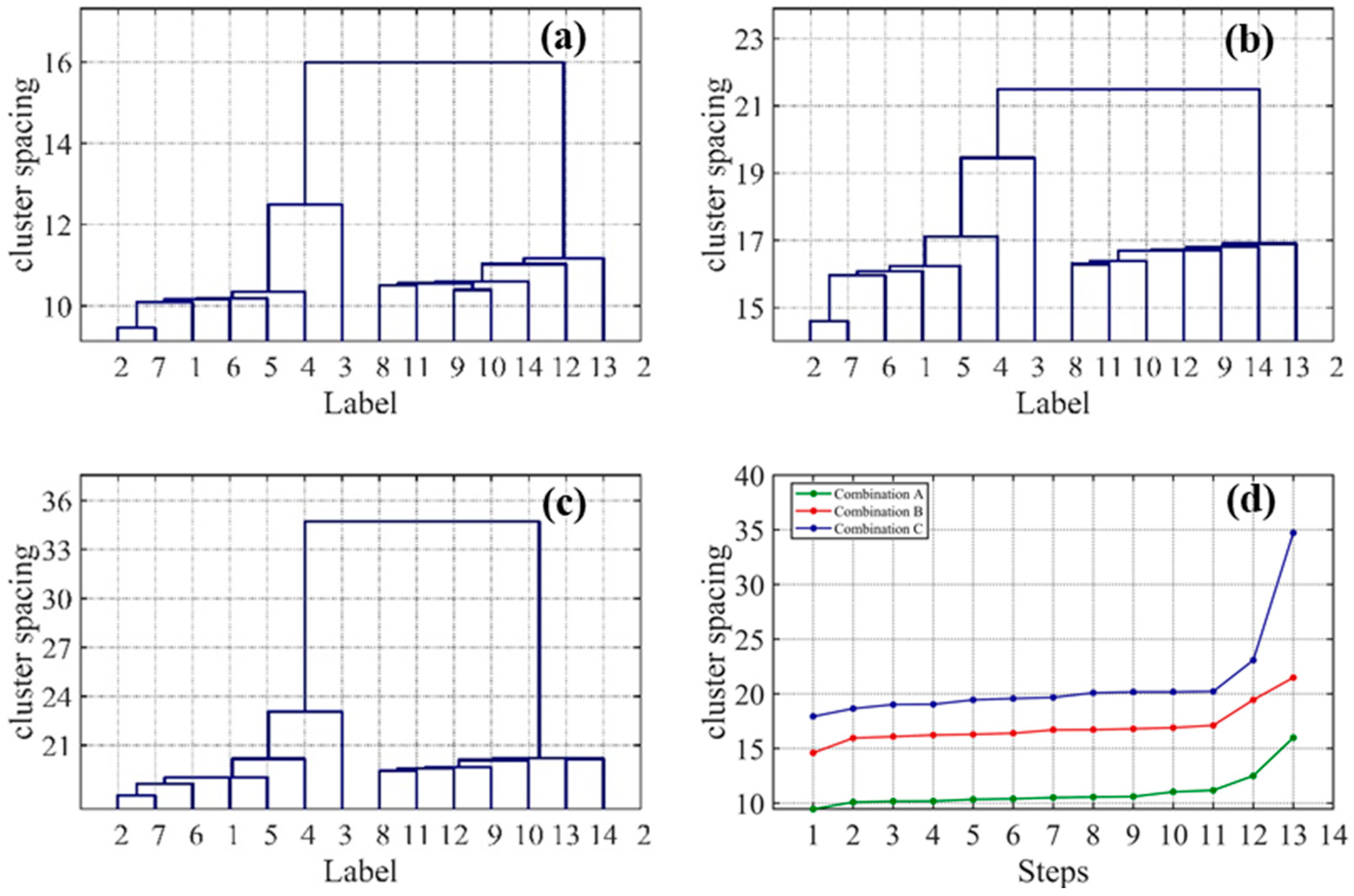
4.1. Clustering of Spectral Polarization Data

Since the sun elevation angle during the 4.2 field experiment was 40 degrees, data collected while the incidence angle in the laboratory is also 40 degrees are picked for analysis. The polarization information at each wavelength was divided into three combination sets: combination A consisting of Stokes data, combination B consisting of Stokes and DOLP, and combination C consisting of Stokes, DOLP, and pBRDF matrix elements. Three different combination matrices were obtained, and half of the vectors in each combination matrix were selected as training set data. Samples were taken from each combined data matrix, and the cluster distance was calculated. The training set was then used in the hierarchical clustering part to run a complete clustering tree as shown in Figure 3a–c.

The goal of clustering is to make data points belonging to the same cluster have a higher degree of similarity, and data points belonging to different clusters have a higher degree of difference, which means that the distance between data points in the same group is small and the distance between groups is as far as possible. Therefore, the steepness of the change in the cluster spacing and intra-cluster distance should be observed as a criterion for judging whether the classification results meet the standard. Figure 3d shows that the boundary points in combination C are steeper than those in combination A and B. From a theoretical analysis point of view, combination C contains richer data information and should have the best results. As a result, the next step is to select combination C as the data set for clustering experiments. Likewise, the cluster distance threshold for combination C when the incident angle is 40° is ε = 32.1446. The overall data profile will be described based on this threshold. This threshold will be used to characterize the entire data profile.

The next step is to calculate the standardized Euclidean distance between all data points to form a square matrix, and set the diagonal to INF(infinity). If the distance between two points is less than the cluster distance threshold, it is established that they are members of the same cluster. The results of the contour characterization are shown in Figure 4, which indicates that the number of clusters calculated based on the cluster distance is 4; hence, the initial parameter K = 4 is substituted into the computation method described in the preceding section. All the initial parameters and overall data obtained above are then fed into the FCM algorithm for the next step of operation.

The data profile parameters and data matrix obtained from the previous HAC were input into the FCM algorithm to obtain the classification results. The Kosko subset measure of the algorithm results was then used to test for ambiguity, and the results were compared and analyzed. Because the amount of data was small, the FCM threshold was set to 0.01 and the maximum number of iterations to 1000. After the clustering algorithm ran and the clusters to which each data point belonged were obtained, the values of all dimensions were first normalized to facilitate observation and comparison of the abscissa. Then, the classification results were projected to the first row of each data in the reorganization matrix above the first dimension and the eighth dimension, forming a two-dimensional clustering scatter diagram as shown in Figure 5. In the figure, data points of the same color belong to the same cluster, which is identified as a material. In the parallel pre-experiment of the six small data sets, the four types of materials were correctly identified and distinguished, and the correct rate of division for the sampling points of each material reached 100%. These experimental results prove the correctness of the algorithm theory and the practicality of implementing it.

Finally, following the Kosko subset measure test, the flag value established to determine whether there is a fuzzy cluster classification mark is 0 for each set of parallel tests, which is displayed as false. Therefore, the precision of the boundary delineation demonstrated by the laboratory experiments is credible. Based on the experimental results and theoretical verification, the proposed algorithm is reasonable and can be used for clustering research in actual scenarios.

4.2. Spectral Polarization Image Clustering Rendering

4.2.1. Random Point Clustering of Spectral Polarization Images

The laboratory experiments have demonstrated the effectiveness of the proposed algorithm in detecting and recognizing space debris targets, particularly for high-dimensional small data sets with large amounts of information. However, traditional single-spectrum, single-polarization images are unable to directly identify and classify targets. Therefore, field experiments are necessary to capture real spectral images of space targets in actual scenarios to validate the robustness of the algorithm.

The algorithm proposed in this paper must rely on the material’s own spectral polarization characteristics, making full use of characteristic parameters that can accurately characterize the spectral polarization characteristics of the space debris. Through the selection of different data combinations, it has been proven through experiments that the optimal data set combination is selected, which is consistent with the results of the characteristic data. Ultimately, the combination of Stokes and DOLP data is chosen as the final data set. Figure 6 depicts the hierarchical clustering tree and line graph of cluster distance in the experimental field spectral polarization characteristic data, from which the critical value of cluster distance ε = 24.9133 is derived. Using this threshold, clustering continues. However, due to the large amount of data, it is not intuitive to directly draw the cluster diagram. According to the clustering result itself, the number of clusters is calculated to be 6.

The scatter diagram in Figure 7a shows the projection of the data vector’s first dimension and 1560th dimension based on the clustering algorithm, and it demonstrates that the six types of points can be separated normally. After setting the threshold, the objective function decreases with each iteration. When the FCM iteration threshold is set to 0.001, the change trend of the objective function J with the number of iterations is displayed in Figure 7b. From the figure, it is evident that the objective function eventually converges to the approximate global optimal value with the increase of the number of iterations, and the decline speed is fast. The convergence is accomplished in 21 iterations, demonstrating the effectiveness of the algorithm developed in this research.

In this paper, the proposed data combination was compared with two classical clustering algorithms: the k-means clustering algorithm and the coalescent upward HAC clustering method. The parameters, such as prior cluster number and prior cluster center, were applied to the two classical algorithms, and the standardized Euclidean distance was used as the vector distance metric. The comparison of the running results of the three algorithms is shown in

Table 2. Three different algorithm cluster results comparison.

Algorithm	Total Points	Correct Points	Recognition Rates
K-means	726	551	75.90%
HAC	726	604	83.20%
Ours	726	726	100%

. The high accuracy of the fusion algorithm is due to the fact that it does not directly assign a certain numerical point to a certain division from the calculation of a certain level like the classical algorithms. Instead, it calculates the degree of membership of the point relative to the cluster after the final convergence. The algorithm flow structure reveals that the k-means algorithm has a time complexity of O(N), but the coalescent upward HAC algorithm has a time complexity of O(N3). With the sample size N being 726 in this paper, the number of iterations of the k-means algorithm should be an integer multiple of 726 (more than double), while the number of iterations of the HAC method is a multiple of the cube of 726. The proposed HAC-FCM algorithm only requires 21 iterations. Therefore, compared with the classical algorithms, the fusion algorithm can obtain clustering results more efficiently and accurately.

4.2.2. Spectral Polarization Image Rendering

In the previous section, points for six materials in the image were randomly selected, and a good clustering result was obtained. In this section, the proposed HAC-FCM algorithm is used to cluster the actual image at the pixel level, and the clustering results are assigned colors, which provides a more intuitive view compared to the polarized grayscale image at each characteristic band. Finding equally spaced single-wavelength images, 11 wavelengths (ranging from 372 nm to 757 nm) are selected from the spectral image. The operation is performed on the image, and the value of the Stokes vector and Dolp are calculated from the intensity value of each pixel to form a three-dimensional reconstruction matrix. Dimensionality reduction was performed on the matrix before applying the fusion algorithm. For the space debris material part in the image, the cluster center obtained in Section 4.2.1 was used as the initial value. After clustering each pixel, the results were color-coded and re-projected onto the original image pixel range to produce the final rendering.

The physical sample of the field experiment is depicted in Figure 8a. The image size of the experiment was 325 × 250, and pixels were colored based on different intensity values. The resulting coloring of the original image at an incident polarization angle of 135° and a wavelength of 442 nm is shown in Figure 8b, with similar results obtained for the other wavelengths. It can be seen that due to high noise interference of background pixels during shooting, the classification effect may be poor. To remove image noise, the Full Average Filter (FAF) method was used to denoise the image, with a filter kernel of 9 × 9 pixels used to smooth the original image. The resulting coloring of the filtered image is shown in Figure 8c, which shows that the background noise is significantly reduced after using the mean filtering method.

Clustering algorithm processing is performed on the image after denoising. As the dataset is large and fuzzy, the FCM threshold is adjusted to 10⁻⁵, while the maximum number of iterations remains 1000. After obtaining the clustering result, the result is colored and reshaped from a one-dimensional vector to the original image shape, and the coloring result is output as an image. The result of denoising image clustering is shown in Figure 9. The image demonstrates that, following mean filtering, the fusion method is able to categorize the filtered image extremely well, with excellent border characteristics. Although there are seven different types of color blocks in the result graph, the algorithm unfortunately recognizes the two coating materials as the same material and separates the material’s outside circle into another category. This is due to the fact that both coating materials are white and have similar surface topography (as shown in Figure 8a), which results in very similar polarization behaviors of the two materials.

The image rendering shows that, except for the very thin iron sheet material, there is a circle of yellow edges around the other material images. This is because the polarization characteristics are extremely sensitive to changes in the material structure, and the thickness of the material cannot be neglected. At the edge where the debris material is in contact with the background, the sudden change in thickness causes a change in its polarization properties. This difference is greater than the difference in polarization properties between the two coatings, which leads the fusion algorithm to group the two coatings together in one class, and the edge as one class. The “edge effect” of the polarization properties was also confirmed by this finding. This effect is brought about by the thickness of the material. Since this effect is caused by the thickness of the material, it is obvious that the edge circle also belongs to the material, so the image is re-rendered, and the result is shown in Figure 10. The clustering results of six space debris materials and one background material in the image are summarized in

Table 3. Analysis of various materials cluster results.

Material	Silver Insulation	Golden Insulation	SR107/S781	Aluminum Block	Iron Sheets	Background Material	Total
error points	1	0	605	1314	3	0	1923
false alarm rate	0.0487%	0	13.67%	39.31%	0.12%	0	3.08%
recognition rates	77.73%	69.71%	86.60%	100%	100%	100%	96.92%

. After denoising the image, the overall false alarm rate of the fusion algorithm is only 3.08%, and the accuracy rate can reach 96.92%. The algorithm still has a good operation effect on pixel clustering, and its universality and robustness have been tested. It can be observed from Figure 9 and Figure 10 that the edges of the four other materials are erroneously classified as aluminum materials, and a circular region inside the thermal insulation cladding material is identified as coating material. This is because the edges of the materials have a significant effect on the polarization characteristics, causing these points to be misclassified as other materials. The relatively high false alarm rate of the aluminum and coating materials in Table 3 is also indicative of this issue. Recognizing these patterns will be the focus of our future work to enhance the fusion algorithm.

5. Discussion and Operational Applications

In this section, the spectral and polarization characteristics of space debris are studied using selected feature parameters. The characteristics of spectral polarization data are analyzed, with a focus on discussing the limitations of the HAC and FCM algorithms when used separately. The suitability of these algorithms for spatial target data characteristics is also examined. Finally, the limitations of the algorithm and possible future research directions are discussed.

Figure 11 depicts the spectrum curves of six types of space debris materials. As shown in the figure, there is little variation in the wavelengths of the characteristic peaks obtained from different materials. Moreover, the commonly used characteristic parameter half-wave width cannot clearly distinguish the spectral characteristics of different materials. Therefore, spectral characteristic data cannot be used as a basis for directly distinguishing space debris materials. Figure 12 and Figure 13 directly classify space debris materials based on their Stokes vector and degree of polarization, respectively. However, it can be observed that the classification results are not satisfactory.

The spectral polarization characteristics of space debris possess multidimensional, hierarchical, and fuzzy features, posing a challenge for effective data clustering. In this regard, we propose the HAC-FCM algorithm, which is a clustering approach that integrates the HAC and FCM clustering techniques. The HAC algorithm is used to determine the initial cluster centers and cluster distances by recursively dividing the data into subsets until each subset contains only one data point. This hierarchical clustering strategy is well-suited for spatial fragmented spectral polarimetric data, which often exhibit complex hierarchical structures across multiple scales. Meanwhile, the FCM algorithm assigns data points to different categories with varying degrees of membership to address the fuzziness of the data.

By integrating the HAC and FCM clustering techniques, the HAC-FCM algorithm proposed in this study effectively addresses the multi-scale, hierarchical, and fuzzy features of spatial fragmented spectral polarimetric data. Specifically, the HAC algorithm is used to recursively divide the data into subsets, followed by FCM clustering on each subset to obtain the final clustering result. However, it is worth noting that the HAC-FCM algorithm may encounter computational efficiency issues when dealing with large data volumes and dimensions, highlighting the importance of carefully selecting the fuzzy index to achieve optimal clustering results. Moreover, expert interpretation may be required to fully understand the clustering outcomes in domain-specific applications.

In order to address these limitations, further research could investigate the potential of integrating other clustering algorithms or including additional spectral and polarization features to enhance the accuracy and computational efficiency of clustering space debris data. It should be noted that the HAC-FCM algorithm has wide-ranging applications in diverse fields, such as remote sensing, image processing, and machine learning. Thus, it has significant potential to advance various scientific and technological domains.

6. Conclusions

In this paper, we proposed a novel fused clustering algorithm that combines polarization and spectral information for the optical detection and identification of space debris targets. Our algorithm achieved a high classification accuracy of 96.92% for six types of samples and outperformed classical methods in an actual scene. The combination of HCA and FCM algorithms provided a stable and robust initial state for the FCM algorithm, thereby improving the effectiveness, adaptability, accuracy, and robustness of clustering for multidimensional space debris datasets. The proposed clustering method demonstrates superior performance in distinguishing spatial target materials with different spectral polarization properties, fully utilizing color discrimination ability, and providing a favorable output format for human vision. Our research provides a better theoretical basis and practical results for space debris detection and identification. In the future, the proposed method has the potential to be further improved with more advanced algorithms as better instruments become available and larger datasets of space objects become available.

References

1. Liou, J.C. USA Space Debris Environment, Operations, and Research Updates. In Proceedings of the 53rd Session of the Scientific and Technical Subcommittee Committee on the Peaceful Uses of Outer Space, United Nations, Vienna, Austria, 15–26 February 2016. [Google Scholar]
2. Jahirabadkar, S.; Pande, P.; R., A. A Survey on Image Processing based Techniques for Space Debris Detection. In Proceedings of the 2022 IEEE Bombay Section Signature Conference (IBSSC), Mumbai, India, 8–10 December 2022; pp. 1–6. [Google Scholar]
3. Jiang, C.; Tan, Y.; Qu, G.; Lv, Z.; Gu, N.; Lu, W.; Zhou, J.; Li, Z.; Xu, R.; Wang, K.; et al. Super diffraction limit spectral imaging detection and material type identification of distant space objects. Opt. Express 2022, 30, 46911–46925. [Google Scholar] [CrossRef] [PubMed]
4. Tapia, S.; Beavers, W.I.; Cho, Y.K. Photopolarimetric observations of satellites. Proc. SPIE 1990, 1317, 252–262. [Google Scholar]
5. Culp, R.D.; Gravseth, I.J. Space-debris identification using optical calibration of common spacecraft materials. J. Spacecr. Rocket. 2015, 33, 262–266. [Google Scholar] [CrossRef]
6. Ratliff, B.M.; Lemaster, D.A.; Mack, R.T.; Villeneuve, P.V.; Weinheimer, J.J.; Middendorf, J.R. Detection and tracking of RC model aircraft in LWIR microgrid polarimeter data. In Polarization Science and Remote Sensing V; SPIE: Bellingham, WA, USA, 2011. [Google Scholar]
7. Namer, E.; Shwartz, S.; Schechner, Y.Y. Skyless polarimetric calibration and visibility enhancement. Opt. Express 2009, 17, 472–493. [Google Scholar] [CrossRef] [Green Version]
8. Chun, C.S.L.; Sadjadi, F.A. Polarimetric laser radar target classification. Opt. Lett. 2005, 30, 1806–1808. [Google Scholar] [CrossRef]
9. Zhang, X.; Zhu, J.; Zong, K.; Huang, L.; Zhai, L.; Zhang, Y.; Wang, H.; Zhang, N.; Cai, Y. Exact optical path difference and complete performance analysis of a spectral zooming imaging spectrometer. Opt. Express 2022, 30, 39479–39491. [Google Scholar] [CrossRef]
10. Saxena, A.; Prasad, M.; Gupta, A.; Bharill, N.; Patel, O.P.; Tiwari, A.; Er, M.J.; Ding, W.; Lin, C. A review of clustering techniques and developments. Neurocomputing 2017, 267, 664–681. [Google Scholar] [CrossRef] [Green Version]
11. Tao, Z.; Huiling, L. Clustering algorithm research advances on data mining. Comput. Eng. Appl. 2012, 48, 100–111. [Google Scholar]
12. Bezdek, J.C. Pattern Recognition with Fuzzy Objective Function Algorithms; Plenum Press: New York, NY, USA, 1981. [Google Scholar]
13. Bezdek, J.C.; Ehrlich, R.; Full, W. FCM: The fuzzy c-means clustering algorithm. Comput. Geosci.-UK 1984, 10, 191–203. [Google Scholar] [CrossRef]
14. Askari, S. Fuzzy C-Means clustering algorithm for data with unequal cluster sizes and contaminated with noise and outliers: Review and development. Expert Syst. Appl. 2021, 165, 113856. [Google Scholar] [CrossRef]
15. Havens, T.C.; Bezdek, J.C.; Leckie, C.; Hall, L.O.; Palaniswami, M. Fuzzy c-Means Algorithms for Very Large Data. IEEE T. Fuzzy Syst. 2012, 20, 1130–1146. [Google Scholar] [CrossRef]
16. Ji, B.; Hu, X.; Ding, F.; Ji, Y.; Gao, H. An effective color image segmentation approach using superpixel-neutrosophic C-means clustering and gradient-structural similarity. Optik 2022, 260, 169039. [Google Scholar] [CrossRef]
17. Wu, C.; Peng, S. Robust interval type-2 kernel-based possibilistic fuzzy clustering algorithm incorporating local and non-local information. Adv. Eng. Softw. 2023, 176, 103377. [Google Scholar] [CrossRef]
18. Bentabet, L.; Zhu, Y.M.; Dupuis, O.; Kaftandjian, V.; Babot, D.; Rombaut, M. Use of fuzzy clustering for determining mass functions Dempster-Shafer theory. In 2000 5th International Conference on Signal Processing Proceedings, Vols I–III; Baozong, Y., Xiaofang, T., Eds.; IEEE: New York, NY, USA, 2000; pp. 1462–1470. [Google Scholar]
19. Xu, W.; Tang, C.; Xu, M.; Lei, Z. Fuzzy c-means clustering based segmentation and the filtering method for discontinuous ESPI fringe patterns. Appl. Opt. 2019, 58, 1442–1450. [Google Scholar] [CrossRef] [PubMed]
20. Wu, C.; Guo, X. A novel interval-valued data driven type-2 possibilistic local information c-means clustering for land cover classification. Int. J. Approx. Reason. 2022, 148, 80–116. [Google Scholar] [CrossRef]
21. Yang, L.; Zenian, S.; Zakaria, R. Image Enhancement Method based on an Improved Fuzzy C-Means Clustering. Int. J. Adv. Comput. Sci. Appl. 2022, 13, 855–859. [Google Scholar] [CrossRef]
22. Wen, Y.; He, L.; Von Deneen, K.M.; Lu, Y. Brain tissue classification based on DTI using an improved Fuzzy C-means algorithm with spatial constraints. Magn. Reson. Imaging 2013, 31, 1623–1630. [Google Scholar] [CrossRef]
23. Al-Saeed, Y.; Gab-Allah, W.A.; Elmogy, M. Fuzzy C-Means Based CAD Sytem for Liver Tumors Segmentation from CT Scans. In Proceedings of the 2022 18th International Computer Engineering Conference (ICENCO), Cairo, Egypt, 29 December 2022; Volume 1, pp. 44–49. [Google Scholar]
24. Mohammdian-Khoshnoud, M.; Soltanian, A.R.; Farhadian, M.; Dehghan, A. Optimization of fuzzy c-means (FCM) clustering in cytology image segmentation using the gray wolf algorithm. BMC Mol. Cell Biol. 2022, 23, 9. [Google Scholar] [CrossRef]
25. Mabel Rani, A.J.; Pravin, A. Multi-objective Hybrid Fuzzified PSO and Fuzzy C-Means Algorithm for Clustering CDR Data. In Proceedings of the 2019 International Conference on Communication and Signal Processing (ICCSP), Chennai, India, 4–6 April 2019. [Google Scholar]
26. Zhao, W.; Ma, J.; Liu, Q.; Song, J.; Tysklind, M.; Liu, C.; Wang, D.; Qu, Y.; Wu, Y.; Wu, F. Comparison and application of SOFM, fuzzy c-means and k-means clustering algorithms for natural soil environment regionalization in China. Environ. Res. 2023, 216, 114519. [Google Scholar] [CrossRef]
27. Li, S.; Zhang, J.; Liu, B.; Jiang, C.; Ren, L.; Xue, J.; Song, Y. An Algorithm to Extract the Boundary and Center of EUV Solar Image Based on Sobel Operator and FLICM. Photonics 2022, 9, 889. [Google Scholar] [CrossRef]
28. Bi, S.; Li, Y.; Xu, J.; Liu, G.; Song, K.; Mu, M.; Lyu, H.; Miao, S.; Xu, J. Optical classification of inland waters based on an improved Fuzzy C-Means method. Opt. Express 2019, 27, 34838. [Google Scholar] [CrossRef] [PubMed]
29. Younès, B.; Mohamad, G.; Nistor, G. Collaborative multi-view clustering. In Proceedings of the 2013 International Joint Conference on Neural Networks (IJCNN), Dallas, TX, USA, 4–9 August 2013. [Google Scholar]
30. Ghassany, M.; Bennani, Y. Collaborative Fuzzy Clustering of Variational Bayesian Generative Topographic Mapping. Int. J. Comput. Intell. Appl. 2015, 14, 1. [Google Scholar] [CrossRef]
31. Pedrycz, W. Conditional fuzzy C-means. Pattern Recogn. Lett. 1996, 17, 625–631. [Google Scholar] [CrossRef]
32. Pedrycz, W.; Hirota, K. A consensus-driven fuzzy clustering. Pattern Recogn. Lett. 2008, 29, 1333–1343. [Google Scholar] [CrossRef]
33. Roh, S.; Oh, S.; Pedrycz, W.; Seo, K.; Fu, Z. Design methodology for Radial Basis Function Neural Networks classifier based on locally linear reconstruction and Conditional Fuzzy C-Means clustering. Int. J. Approx. Reason. 2019, 106, 228–243. [Google Scholar] [CrossRef]
34. Ding, Y.; Fu, X. Kernel-based fuzzy c-means clustering algorithm based on genetic algorithm. Neurocomputing 2016, 188, 233–238. [Google Scholar] [CrossRef]
35. Ding, W.; Feng, Z.; Andreu-Perez, J.; Pedrycz, W. Derived Multi-population Genetic Algorithm for Adaptive Fuzzy C-Means Clustering. Neural Process. Lett. 2022. [Google Scholar] [CrossRef]
36. Murtagh, F.; Contreras, P. Algorithms for hierarchical clustering: An overview. Wires. Data Min. Knowl. 2012, 2, 86–97. [Google Scholar] [CrossRef]
37. Govender, P.; Sivakumar, V. Application of k-means and hierarchical clustering techniques for analysis of air pollution: A review (1980–2019). Atmos. Pollut. Res. 2020, 11, 40–56. [Google Scholar] [CrossRef]
38. Ran, X.; Xi, Y.; Lu, Y.; Wang, X.; Lu, Z. Comprehensive survey on hierarchical clustering algorithms and the recent developments. Artif. Intell. Rev. Int. Sci. Eng. J. 2022, 1–46. [Google Scholar] [CrossRef]
39. Dinh, D.; Fujinami, T.; Huynh, V. Estimating the Optimal Number of Clusters in Categorical Data Clustering by Silhouette Coefficient; Springer Singapore Pte. Limited: Singapore, 2019; Volume 1103, pp. 1–17. [Google Scholar]
40. Priest, R.G.; Gerner, T.A. Polarimetric BRDF in the Microfacet Model: Theory and Measurements. In Proceedings of the Meeting of the Military Sensing Symposia Specialty Group on Passive Sensors, Ann Arbor, MI, USA, 1 March 2000. [Google Scholar]
41. Hyde, M.T.; Schmidt, J.D.; Havrilla, M.J.; Cain, S.C. Enhanced material classification using turbulence-degraded polarimetric imagery. Opt. Lett. 2010, 35, 3601–3603. [Google Scholar] [CrossRef] [PubMed]
42. Wang, K.; Zhu, J.; Liu, H.; Du, B. Expression of the degree of polarization based on the geometrical optics pBRDF model. J. Opt. Soc. Am. A Opt. Image Sci. Vis. 2017, 34, 259–263. [Google Scholar] [CrossRef] [PubMed]
43. Hyde, M.T.; Schmidt, J.D.; Havrilla, M.J. A geometrical optics polarimetric bidirectional reflectance distribution function for dielectric and metallic surfaces. Opt. Express 2009, 17, 22138–22153. [Google Scholar] [CrossRef] [PubMed]
Figure 1. Schematic diagram of HAC-FCM clustering algorithm structure.
Applsci 13 04754 g001
Figure 2. Typical target material polarization spectrum scattering characteristics test system. PSA, polarization state detector, PSG, polarization state generator, P1 and P2, linear polarizer, SF, spectral filter.
Applsci 13 04754 g002
Figure 3. Data training set hierarchical cluster tree and cluster distance folding line change diagram. (a) Combination A Stokes dataset (b) Combination B Stokes and DOLP dataset (c) Combination C Stokes, DOLP, and pBRDF matrix element dataset (d) Combining hierarchical cluster distance folding line change diagram with data.
Applsci 13 04754 g003
Figure 4. The data contour port at incident angle is 40°.
Applsci 13 04754 g004
Figure 5. FCM algorithm in a 2D scatter plot.
Applsci 13 04754 g005
Figure 6. Training set hierarchical clustering tree and cluster distance line diagram. (a) Stokes and DOLP combination data set hierarchical cluster tree (b) Data combination layer cluster distance folding line change diagram.
Applsci 13 04754 g006
Figure 7. Results scattered point diagram and iteration change diagram. (a) FCM algorithm in a 2D scatter plot (b) FCM target function J iteration change diagram.
Applsci 13 04754 g007
Figure 8. (a) Physical picture, (b) color map, (c) color map after denoising.
Applsci 13 04754 g008
Figure 9. Coloring result of clustering.
Applsci 13 04754 g009
Figure 10. Image after edge processing.
Applsci 13 04754 g010
Figure 11. Spectral characteristic curve of space debris material.
Applsci 13 04754 g011
Figure 12. Spatial distribution of normalized Stokes vectors of space debris.
Applsci 13 04754 g012
Figure 13. Probability density distribution characteristics of the degree of polarization for different space debris materials.
Applsci 13 04754 g013