
Genetic Algorithms Optimized Adaptive Wireless Network Deployment

Department of Computer Science and Engineering, University of Nevada Reno, NV 89512, USA
*
Author to whom correspondence should be addressed.
Appl. Sci. 2023, 13(8), 4858; https://0-doi-org.brum.beds.ac.uk/10.3390/app13084858
Submission received: 15 March 2023
/
Revised: 5 April 2023
/
Accepted: 7 April 2023
/
Published: 12 April 2023
(This article belongs to the Special Issue Evolutionary Computation: Theories, Techniques, and Applications)
Abstract
:Advancements in UAVs have enabled them to act as flying access points that can be positioned to create an interconnected wireless network in complex environments. The primary aim of such networks is to provide bandwidth coverage to users on the ground in case of an emergency or natural disaster when existing network infrastructure is unavailable. However, optimal UAV placement for creating an ad hoc wireless network is an NP-hard and challenging problem because of the UAV’s communication range, unknown users’ distribution, and differing user bandwidth requirements. Many techniques have been presented in the literature for wireless mesh network deployment, but they lack either generalizability (with different users’ distributions) or real-time adaptability as per users’ requirements. This paper addresses the UAV placement and control problem, where a set of genetic-algorithm-optimized potential fields guide UAVs for creating long-lived ad hoc wireless networks that find all users in a given area of interest (AOI) and serve their bandwidth requirements. The performance of networks deployed using the proposed algorithm was compared with the current state of the art on several experimental simulation scenarios with different levels of communication among UAVs, and the results show that, on average, the proposed algorithm outperforms the state of the art by to .
1. Introduction
UAVs are gaining traction as a useful tool in many different domains, including search and rescue [1,2], surveillance [3], cargo transport [4], surveying and mapping [5,6], disaster relief [7], and Internet of Things (IoTs) [8,9]. This paper specifically focuses on the search and rescue application domain, where the challenge is to establish an on-demand UAV-based wireless network in remote areas or when existing communication infrastructure fails to operate due to natural calamity or stress on the existing network.
In network deployment, a set of UAVs is deployed within a given AOI to provide wireless connectivity to ground users for an extended period. For known user distributions, centralized network deployment algorithms are used to generate wireless mesh networks. However, deploying networks to serve users with unknown distributions is challenging. While many techniques for network deployment in unknown environments have been proposed in the literature, generalizability and real-time adaptation to uniformly and non-uniformly distributed users remain challenges. This paper aims to present an approach that is generalizable to different types of user distributions and adaptable to users’ requirements.
The deployment of a UAVs-based ad hoc network in unknown environments is usually divided into two sub-challenges. The first challenge is to find the users’ distribution. This is a relatively easier task and several geometrical-based algorithms [10,11] have been proposed in the literature to deploy static networks. The second challenge is to adaptively re-deploy UAVs in real-time to connect users with the command center [12], which is an NP-hard problem. Compared to static networks, less work exists on the part of the re-configuration of networks that adapts to users’ requirements in real-time. The reconfiguration of networks is difficult due to the limited communication range between UAVs, limited battery life of UAVs, and various environmental conditions. This problem needs more attention and has many real-world applications.
This paper presents a two-phase approach to network deployment, where potential fields (PFs) govern the movement of UAVs. In the first phase, a set of potential field parameters is derived for static network deployment. For the second phase, a genetic optimization approach is presented, genetic adaptive network deployment (GANet), that optimally deploys UAVs to create an ad hoc wireless network. The problem has been formulated as an optimization problem with the aim of maximizing the sum of bandwidth coverage provided to users and the longevity of the deployed network. To provide more bandwidth coverage, UAVs move under the influence of a set of potential fields toward users in the AOI, and to increase the longevity of the deployed network, UAVs position themselves to share the bandwidth demanded by users while maintaining connectivity to the command center.
In the simulation, each UAV’s movement is controlled by a set of potential fields, where each potential field has two parameters [13,14], and these parameters can be tuned to achieve the desired behavior from UAVs. However, searching for parameters that optimally control the movement of UAVs to create optimal wireless networks is difficult for two reasons: (1) due to the non-linearity of potential fields and (2) because of the large search space. In the literature, it has been shown that genetic algorithms (GAs) work well with non-linear problems and problems with a large search space. Thus, a genetic algorithm has been used to evolve solutions. The potential field parameters are encoded in a real-valued chromosome and the GA searches through the space of potential field parameters. Note that other search algorithms can also be applied for searching through this space, and, in the results section, the GAs performance is compared with two other search algorithms. The network deployment problem is divided into two phases to deal with two different problems: (1) the search phase, for searching users on the ground by deploying a static network, and (2) the service phase, to reconfigure a deployed network adaptively to better serve users.
The proposed two-phase approach deploys networks in real-time and adapts to users’ requirements. However, this does not guarantee generalizability and robustness. To obtain generalizable solutions (a set of potential field parameters) that work for unknown user distributions, four different training scenarios with varying user distributions (uniform and non-uniform) were generated. The aim is to tune the potential field parameters to be distribution-agnostic and enable UAVs to better serve users. To measure the generalizability and robustness of the proposed approach, the performance of the best evolved solution was measured on 100 different test scenarios with varying user distributions. These test scenarios were designed to simulate real-world scenarios and provide a comprehensive evaluation of the approach’s performance.
The experimental results show that the networks deployed using the best solution evolved using GANet on four training scenarios outperformed the networks deployed using the current best network deployment algorithm, adaptive triangular network deployment (ATRI) [15], on training scenarios. More importantly, it was found that this performance advantage also holds over the never before seen 100 test scenarios. Furthermore, different levels of information exchange between UAVs have been considered to measure the differences in the performance of deployed networks. Specifically, we compared the performance of networks deployed considering one-hop (neighbor) UAV-to-UAV communication with two-hop (neighbor’s neighbors) communication. The results show that the performance of two-hop GANet is statistically significantly better than one-hop GANet and ATRI.
This work makes two significant contributions. First, we propose a unified approach that can be used for both static and dynamic network deployment. Second, our proposed approach is adaptive, generalizable, and demonstrates a superior performance compared to the current state-of-the-art network deployment algorithms when deploying dynamic networks. The remainder of this paper is organized as follows. Section 2 describes prior work in mesh networks and potential fields-based UAVs movement. Section 3 sets up the problem and Section 4 describes the UAV’s movement model under the influence of potential fields. Section 5 explains the two-phase proposed algorithm. The experimental setup and results constitute Section 6 and the last section provides conclusions.
2. Related Work
Many challenges arise when deploying a wireless mesh network in unknown environments. Optimal UAV placement, fast deployment, maintaining a mesh network connected to a command center, minimizing the number of deployed UAVs, maximizing the lifetime of deployed networks, routing [16], and channel allocation all present significant challenges [12,17]. In the literature, several techniques have been introduced for positioning UAVs based on Delaunay triangulation (DT) [15], the circle packing theorem (CPT) [10], and Voronoi diagrams (VDs) [11] to create static networks. A network deployed using DT has no coverage gap while having minimum overlap between UAV’s sensing areas. CPT computes the locations of UAVs while ensuring no overlap and a minimum coverage gap. A VD divides the entire AOI into different segments and places a UAV in each segment to provide bandwidth coverage to users. Such static network deployment is primarily used for area coverage. Lam [18] deployed a heterogeneous sensor network using circle packing by filling the given AOI with circles of different radii corresponding to different UAV types. Lyu [19] proposed a placement optimization technique that first deploys a network using CPT and then adjusts the altitude of deployed UAVs to cover the entire AOI with fewer UAVs while providing wireless coverage to ground terminals. These are computational geometry model-based techniques used to compute the position of UAVs and they do not adapt to users’ locations or bandwidth requirements. Our proposed GANet, on the other hand, adapts to both while maximizing network longevity.
Researchers have presented modifications to make static networks more adaptive to users’ requirements. Ming [15] introduced the state-of-the-art adaptive triangular network deployment algorithm, ATRI, by taking inspiration from Delaunay triangulation. Using one-hop neighbor’s state information, ATRI generates a mesh network by adjusting the distance between neighboring UAVs in order to better share bandwidth within a given AOI. Unlike our approach, ATRI, however, does not work well when users are distributed non-uniformly or clustered in groups. In [20], the authors initially deployed UAVs using CPT and presented a mathematical model to adjust the altitude of deployed UAVs for near-optimal coverage. Increasing the altitude of UAVs increases the coverage range but decreases the signal strength, resulting in a poorer coverage quality. In this work, UAVs were deployed at a fixed altitude and only moved in two-dimensional space. Bartolini [21] proposed a Voronoi polygon-based adaptive network deployment algorithm to deploy heterogeneous mobile sensors. The algorithm computes different polygons for different sensors and moves a sensor only when the sensor does not detect any users on the ground. Amar [22] presented a dynamic algorithm to serve a sub-region within the AOI that requires more bandwidth. Both of these papers assume a uniform users’ distribution whereas this paper deals with non-uniform users’ distribution as well. Section 5 of this paper describes how to use potential fields to deploy networks in the first phase to mimic DT and then re-deploy UAVs using a set of potential fields optimized by a genetic algorithm to maximize the bandwidth coverage and longevity during the second phase.
The potential-field-based real-time control of mobile agents was first introduced by Khatib [23]. Owing to their simplicity, many researchers used potential fields to control UAVs and other autonomous agents in different domain-specific tasks [14,24,25]. Howard [26] used potential fields to deploy mobile sensor networks to cover an area. In their approach, an agent experienced repelling potential fields based on the distance from other agents and obstacles and moved toward unexplored areas. Poduri [27] introduced a mobile network deployment algorithm with the constraint that each agent has at least K neighbors, where K is a user-defined number. Poduri’s paper provides evidence that potential fields can be used to generate a static mesh network similar to that generated by Delaunay triangulation or the circle packing theorem. Zhao [28] presented a centralized algorithm and a potential-field-based distributed algorithm for UAV deployment while maintaining connectivity among UAVs. However, the authors considered only two different types of user distributions: uniformly random and in three clusters spread around the AOI with a command center in the middle. All of these approaches work well in a relatively uniform distribution of users but not as well when users are distributed non-uniformly.
Machine-learning-based approaches have been used for optimal UAV deployment [29]. Genetic algorithms have been particularly popular for deploying static networks in the AOI. For example, Reina [30] presented a multi-layout multi-subpopulation genetic algorithm that optimizes coverage, fault-tolerance, and redundancy. Dina [31] used a variable-length genetic algorithm to optimize the area coverage and deployment cost using non-homogeneous sensors. Subash [32] proposed a GA-based deployment algorithm that maximizes longevity by activating and deactivating sensor nodes. Ruetten [33] developed a GA-based area optimizer that maximizes the covered area. Aziz [34] used a hybrid of particle swarm optimization (PSO) and Voronoi diagrams to find the optimal deployment of nodes/UAVs for best coverage, and Li [35] used the artificial bee colony (ABC) algorithm to maximize throughput. Abdulrab [36] used the Harris hawk’s optimization (HHO) algorithm to find the optimal sensor placement for maximum coverage and connectivity. These approaches typically encode locations in chromosomes and are not generalizable. Table 1 compares different network deployment methods based on their control mechanism, applicability toward uniform and non-uniform user distributions, and generalizability, providing readers with a clear overview of the current state of research in this field.
Unlike previous works that solely focus on UAV position optimization, this paper introduces a genetic algorithm to evolve potential field parameters that guide real-time collision-free UAV movement toward optimal positions. By fine-tuning the potential parameters, the proposed algorithm can optimally place UAVs regardless of the distribution of users and other UAVs in the area of interest. The resulting UAV network is deployed in real-time and is highly generalizable. This approach not only provides UAV positions but also ensures safe and efficient movement to these positions.
The next section presents the problem formulation, fitness computation, and an elitist genetic algorithm.
3. Problem Formulation
3.1. System Model
The network deployment problem was formulated as an optimization problem to maximize the performance of the network in terms of bandwidth coverage and longevity. Assume that a set of N identical UAVs need to be deployed in a given AOI of with a command center located in the middle at [37]. All UAVs are initially located at the center within a area and fly at a constant altitude of 100 m. Each UAV is equipped with sensors that can detect users on the ground within a ground-sensing range of 100 m and can communicate with its neighbors within an air-to-air communication range of 300 m [22]. A total of m users, each with a position and a bandwidth requirement , are distributed over the AOI. Therefore, the users can be represented by a list of pairs: . These simulation parameters can be easily changed. In the results section, we demonstrate the performance of our proposed algorithm with various AOIs, numbers of UAVs and users, and different user distributions. Additionally, other parameters, such as the range of UAV–UAV communication, range of UAV–user communication, and initial energy, can also be adjusted as needed. This paper treats the network deployment problem as a search problem and thus channel modeling for communication among UAVs and between UAVs and users is a subject for future work.
3.2. Fitness Computation
Assume that each UAV has a limited initial energy of joules and consumes energy while hovering/moving and providing data to users [22]. Intuitively, if more UAVs share the bandwidth demanded by users, the per UAV bandwidth service can be reduced, leading to less energy consumption and longer UAV flight times. Thus, the aim is to deploy UAVs to increase the bandwidth coverage while sharing bandwidth demands. Each UAV is classified as either an active UAV (AU) or an inactive UAV (IU) based on whether or not the UAV is serving a user. If a UAV finds users within its ground-sensing range, , the UAV is an AU; otherwise, it is an IU. The number of AUs is proportional to the network lifetime. The more AUs, the more bandwidth that can be distributed among AUs, leading to less power consumption per AU and thus a longer battery life to stay aloft and keep the network alive. A variable represents the status of UAVs, where is 1 for active UAVs and 0 for inactive UAVs.
Equation (1) calculates the aggregate bandwidth that is provided to users, where i sums over N UAVs and denotes the bandwidth served by the ith UAV. The objective function value increases as the bandwidth coverage expands. In the same vein, Equation (2) tallies the total number of active UAVs, , in the deployed network. As the number of increases, the per AU data rate decreases and the energy consumption decreases as well. To ensure that the bandwidth coverage lasts for an extended period, and are combined in Equation (3) to form the fitness function, where is the bandwidth requirement of the jth user and m is the number of users.
It is worth mentioning that the first and second terms of the fitness function were normalized due to the uncertainty surrounding the maximum bandwidth demand from users and the number of available UAVs for deployment. By normalizing the components of the fitness function, the maximum and minimum values are always confined within a fixed range. The maximum value of each term in the Equation (3) is 1, which limits the fitness value to a range of [0–2]. When computing the objective function using Equation (3), several constraints must be satisfied. Each UAV must be positioned within the specified AOI; thus, the UAV’s x and y coordinates must be . Our simulation used the plane for the horizontal plane, , where , which is the maximum bandwidth a UAV can provide in Mbps [22].
3.3. Genetic Algorithms
A () elitist genetic algorithm shown in Algorithm 1 searches through the space of potential field parameter values, which is encoded in the real-value chromosome. The () elitist genetic algorithm is a variant of the genetic algorithm that combines the best individuals from the parent population and offspring population to form a new population. It uses elitism to ensure that the best individuals are preserved from one generation to the next [38]. In Algorithm 1 , are probabilities of crossover and mutation, g is the number of generations, h is the number of hops for communication between UAVs, is the population size, and is the number of children generated through recombination. A number of prototyping experiments were conducted to explore different and g values, types of selection strategies, crossover types, and mutation algorithms and associated probabilities. Based on these preliminary experiments, simulated binary crossover, polynomial mutation, and binary tournament selection were chosen.
| Algorithm 1 An elitist genetic algorithm |
 |
The aim is to show that the genetic algorithm evolved potential field parameters that work across a wide range of user distributions in the AOI, and the results (Section 6) show that using the average performance over the four training scenarios translates robustly to testing scenarios. The next section explains the UAV’s movement under the influence of potential fields. Subsequently, Section 5 explains how to derive these potential field parameters to deploy a static network in the search phase and how to use GA-tuned parameters to reconfigure the deployed network.
The aim is to evolve high-quality and robust solutions for wireless network deployment. However, earlier work has shown that solutions evolved on one scenario (user distribution) may not be robust [13,39]; that is, potential field parameters evolved on one scenario may over-fit and thus not work well in other scenarios. Therefore, four training scenarios with different user distributions were created to evolve robust solutions, as shown in Figure 1. The genetic algorithm seeks to maximize the average objective function value, computed using Equation (3), over all four scenarios. The robustness of the best-evolved solution was tested on 100 different unseen test scenarios, and three of those are shown in Figure 2.
4. Potential-Field-Based UAV Movement Modeling
Potential fields have been used to guide autonomous agents [14,25] in complex environments and in real-time. This section briefly explains how potential fields guide UAVs. Assume that, initially, N UAVs are placed near the center of the AOI and are hovering at 100 m altitude with zero horizontal speed (). The maximum speed of a UAV is fixed to 15 m/s, with an acceleration of 0.1 . Assume that a UAV (kth) can communicate with n neighbors directly and experience an attractive () and repulsive () potential field based on the distance from each of its neighbors. The vector sum of these potential fields () is given by Equation (4), which provides a heading or direction for the kth UAV () to move along.
In the literature, potential fields of the form have been used to control the movement of autonomous agents [40], where coefficient and exponent are optimizable parameters that determine the field effect. In Equation (4), both and can be substituted by the form of as shown by Equation (5).
In the above equation, is a unit vector pointing from the kth UAV to the ith neighbor and vice-versa for , is the distance between the kth and ith UAVs, are potential field coefficients, and are potential field exponents. The genetic algorithm optimizes these coefficients and exponents to control each UAV’s movement, and ’s direction specifies the kth UAV’s heading to move along. In our model, UAVs change their current heading to this new heading (computed using Equation (5)) instantaneously with velocity () and position () computed using Equation (6).
Since UAVs move under the influence of potential fields, their movement comes to a halt when the resultant field value () reaches zero or falls below a threshold value. So far, the background of the problem, the fitness criteria, training, and testing scenarios, and the UAV’s movement model have been discussed. The next section presents the proposed network deployment algorithm in two phases to deploy on-demand wireless networks.
5. Proposed Network Deployment
The proposed network deployment works in two phases. The first phase deals with static network deployment to find the user distribution in an unknown environment. In the second phase, we present the genetic adaptive network deployment algorithm, GANet (shown in Algorithm 2), which adaptively reconfigures the deployed static network (in the first phase) as per user demand.
| Algorithm 2 Genetic Adaptive Network Deployment (GANet) |
 |
5.1. First Phase: Search
In this phase, UAVs move to cover the entire AOI, also called static network deployment. Potential fields are used to deploy UAVs for maximal area coverage with minimal overlap. This is performed to find the distribution of users within the area.
5.1.1. Derivation of Parameters
To generate a static network using potential fields, the sum of potential fields must be zero; that is, (from Equation (4)) for each UAV. We thus need to find values of such that, when , = as shown by Equation (7). It has been shown that, for , the coverage is optimal [15]. Equation (7) is derived from Equation (4) by substituting .
In the equation, the directions of unit vectors and are opposite to each other ( = ). Earlier work in potential-fields-based movement control has shown that the attractive potential should be proportional to the distance and the repulsive potential field should be inversely proportional to the distance squared to provide collision-free cohesive movement [41,42]; thus, and are set to 1 and −2, respectively.
In the simulation experiment, meters, and Equation (7) shows the relationship between and . Assuming that , we obtain .
5.1.2. Deployment of Static Networks of Different Sizes
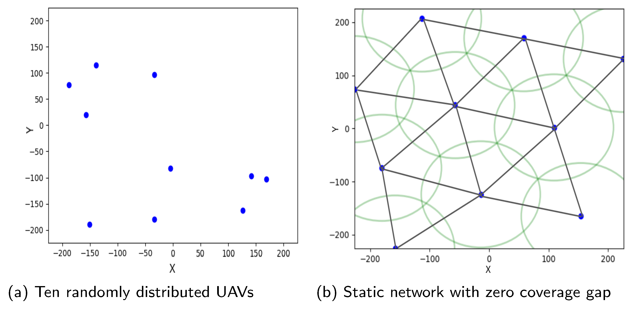
These derived parameters can be used to guide UAVs to create a static network of different sizes. For example, Figure 3a shows 10 randomly distributed UAVs, where each UAV starts at the locations indicated by the blue dots. The UAVs then move under the influence of attractive and repulsive potential fields from neighbors using the above parameters, and Figure 3b shows the resulting static network when the UAVs stop moving. This positioning is identical to Delauney triangulation [15], and this shows that potential-field-based static network deployment can subsume Delaney-triangulation-based network deployment. Furthermore, potential field parameters can also be derived to deploy networks similar to CPT [10]. Note that there exist multiple sets of values of the coefficients and exponents that will result in similar static network deployments.
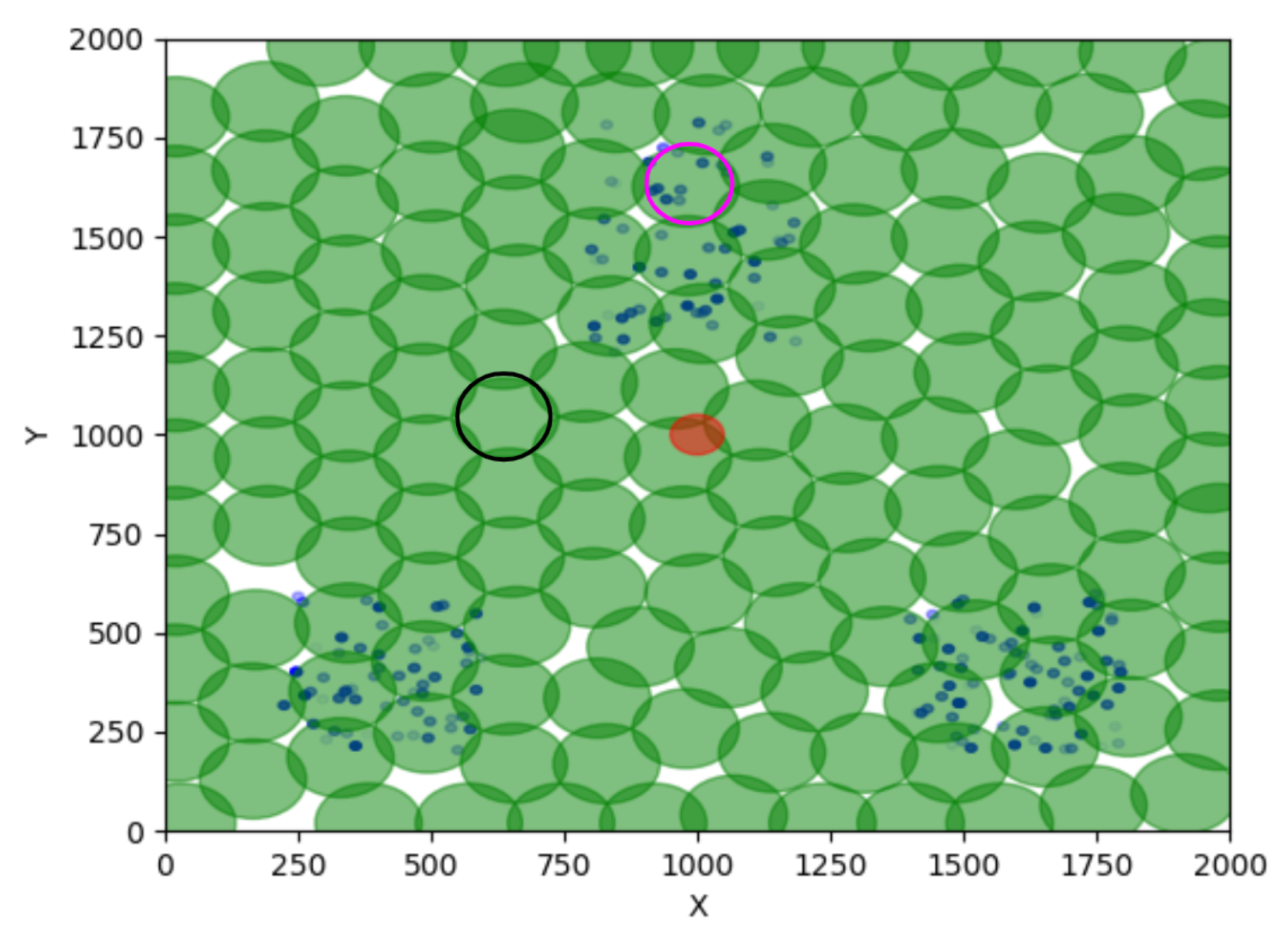
The same parameters can also be used to create static networks with different numbers of UAVs. For example, 156 UAVs are deployed in an AOI of , where UAVs start within an area of near the center of the AOI. The search phase runs for 1500 time steps and Figure 4 shows the UAVs’ positioning (green circles) at the end, where users (blue dots) are distributed in three clusters. Green circles show UAV coverage areas with the UAV in the center of each circle, and the red circle represents the command center. A black circle shows a UAV serving no users within , thus acting as an inactive UAV. Similarly, the magenta circle shows a UAV serving multiple users and is an example of an active UAV. Increasing the number of UAVs that serve the same users leads to bandwidth sharing that decreases the active UAV energy consumption and thus increases the network longevity. The second phase of the network deployment seeks to increase the number of active UAVs by moving UAVs from areas with lower bandwidth requirements (fewer users) to areas with higher bandwidth requirements (more users) while maintaining network connectivity with the command center.
5.2. Second Phase: Service
In this phase, a different set of potential fields optimized by a genetic algorithm re-deploys UAVs to better serve users found in the first phase. The movement of UAVs in the service phase is specified by Algorithm 2, GANet. The algorithm first re-configures the static networks by controlling the movement of UAVs using a set of potential field parameters encoded in a candidate solution and then computes the fitness of the candidate solution.
5.2.1. Re-Configuration of Static Network
In Algorithm 2, MS is the number of training scenarios (4), MT is the maximum simulation time steps (1500), CS is a candidate solution provided by the GA that encodes potential field coefficients and exponents, and h is the number of communication hops allowed between UAVs. At each simulation step (t), every UAV scans for users (AssociateUsers) within to find their positions and bandwidth requirements. The time complexity of this operation is . Similarly, FindNeighbors finds other UAVs within distance and records them as neighbors with the time complexity of . ActivePotentials finds a set of potential fields depending on the hop count (h), and ComputeDir computes the resultant potential field for each UAV by summing all potential fields acting on a UAV using Equation (8).
Next, MoveAll(Dir) moves the kth UAV in the direction of . These three previous functions take a constant time for execution. After time steps, the algorithm computes the fitness for each training scenario by summing the normalized bandwidth coverage and the normalized number of active AUs. Finally, once the evaluation of all four scenarios is over, the algorithm returns the average of these fitness values as the fitness of this candidate solution to the genetic algorithm.
Note that, in Equation (8), h refers to the number of hops for communication. The vector sum of the potential fields for UAV k given by provides a desired heading for the kth UAV to turn toward. Each term in the equation describes a potential field whose parameters need to be optimized. To move the kth UAV toward users, an attractive potential field is generated based on users’ bandwidth requirements (), and to reduce the per UAV bandwidth coverage and save energy, the kth UAV uses an attractive potential field toward neighboring UAVs whose magnitude depends on the neighbor’s bandwidth load (), as shown by Figure 5. At the same time, to avoid collisions, a repulsive potential field, , ensures that UAVs do not collide with each other. This potential field only applies to UAVs that are less than distance away, and we used the Dirac delta function, , to model this, where . When UAV j is less than distance away, then ; otherwise, it is 0. Lastly, when a UAV has no users within and no UAVs within —that is, the UAV is inactive—it moves toward the command center as a default behavior. This is achieved with an attractive potential field () based on the distance to the command center. Here, is another Dirac delta function used to ensure that this potential field only acts on inactive UAVs.
5.2.2. h-hop Network Deployment
To account for the limited communication range of UAVs, Equation (8) is modified for one-hop and two-hop neighbors, resulting in Equations (9) and (10), respectively. These equations represent potential fields in the form of , where the values of the coefficients and exponents are optimized to generate the desired UAV movements.
Here, are the coefficients, are the exponents of the potential fields, is the number of users within the kth UAV sensing range, is the number of one-hop neighbors, and is the number of two-hop neighbors. is the bandwidth required by the ith user and points towards the user. is the bandwidth being served by the jth one-hop neighbor of kth UAV and points toward this neighbor. is the vector difference between the positions of UAV k and UAV j and points from j to k. In the last term, is the vector difference between the command center position and UAV k pointing from k to the command center.
Note that, for and , the kth UAV experiences four and six different potential fields, respectively. In general, for h-hop communication, the kth UAV will experience different potential fields. Since each potential field has two tunable parameters (), a total of potential field parameters will need to be optimized. Due to the non-linearity of potential fields, optimizing their parameters is difficult and thus a genetic algorithm is used. Coefficients and exponents are encoded in chromosomes, where , , and ranges between . Once GA evolved solutions, we compared the deployed network performance using GANet against the performance of the current state-of-the-art ATRI algorithm.
6. Experimental Results and Discussion
This section first evaluates the performance of genetic algorithm parameter tuning on a simple tractable problem and compares it against a random exhaustive search and a hill climber (gradient ascent). Later, we conducted more extensive experiments on 4 training and 100 testing scenarios. In order to carry this out, we created various training and testing scenarios with diverse user distributions using the Unity 3D game engine [43]. The entire simulation was implemented in the language. Since network deployment simulation is computationally expensive, we parallelized the simulation using Open MPI [44] to increase the evaluation speed.
6.1. A Simple Test Problem
Starting with a test problem of deploying 10 UAVs to provide bandwidth coverage to 10 users in a small area of , where the command center is located at , a static network was deployed using the derived potential field parameters. In Figure 6a, blue dots represent users, the red circle is the command center, and green circles show the coverage of UAVs. The objective is to find another set of potential field parameters that can re-configure the static network using one-hop information to maximize the fitness.
Three different search methods were employed to search for optimal potential field parameters that result in the optimum fitness of 2. Note that the maximum fitness according to Equation (3) is 2. Simulation experiments were conducted ten times with different initializations, and the average performance was recorded. All three techniques found optimal solutions and a network deployed using an optimal solution is shown by Figure 6b, where each UAV is serving users and sharing the total bandwidth demanded by users to reduce the per UAV data rate. Figure 6c compares the performance of the three algorithms and shows that the genetic algorithm finds the optimum in significantly fewer evaluations than the others. The genetic algorithm (39) is more than twice as fast as its nearest competitor (92). These results demonstrate the effectiveness of GA for searching potential field parameters. The next subsection discusses the results obtained from the four training scenarios.
6.2. Experiments on Training Scenarios
Experiments were conducted using 156 UAVs and 200 users on four training scenarios. A total of 156 UAVs were selected as they provide sufficient coverage to completely cover the AOI without any gaps in coverage. In each scenario, the simulation ran for 1500 steps, and, in each time step, UAVs moved toward users under the influence of a GA-optimized set of potential fields as given in Algorithm 2. To find GA parameter settings, the population size varied between 10 to 60, the number of generations between 10 to 90, and, through a grid search, a population size of 20 and 20 generations was chosen. Offspring were produced using simulated binary crossover, with a crossover probability of 0.90, and polynomial mutation, with a probability of 0.05 [38].
6.2.1. Comparing the Performance of Evolved Solutions
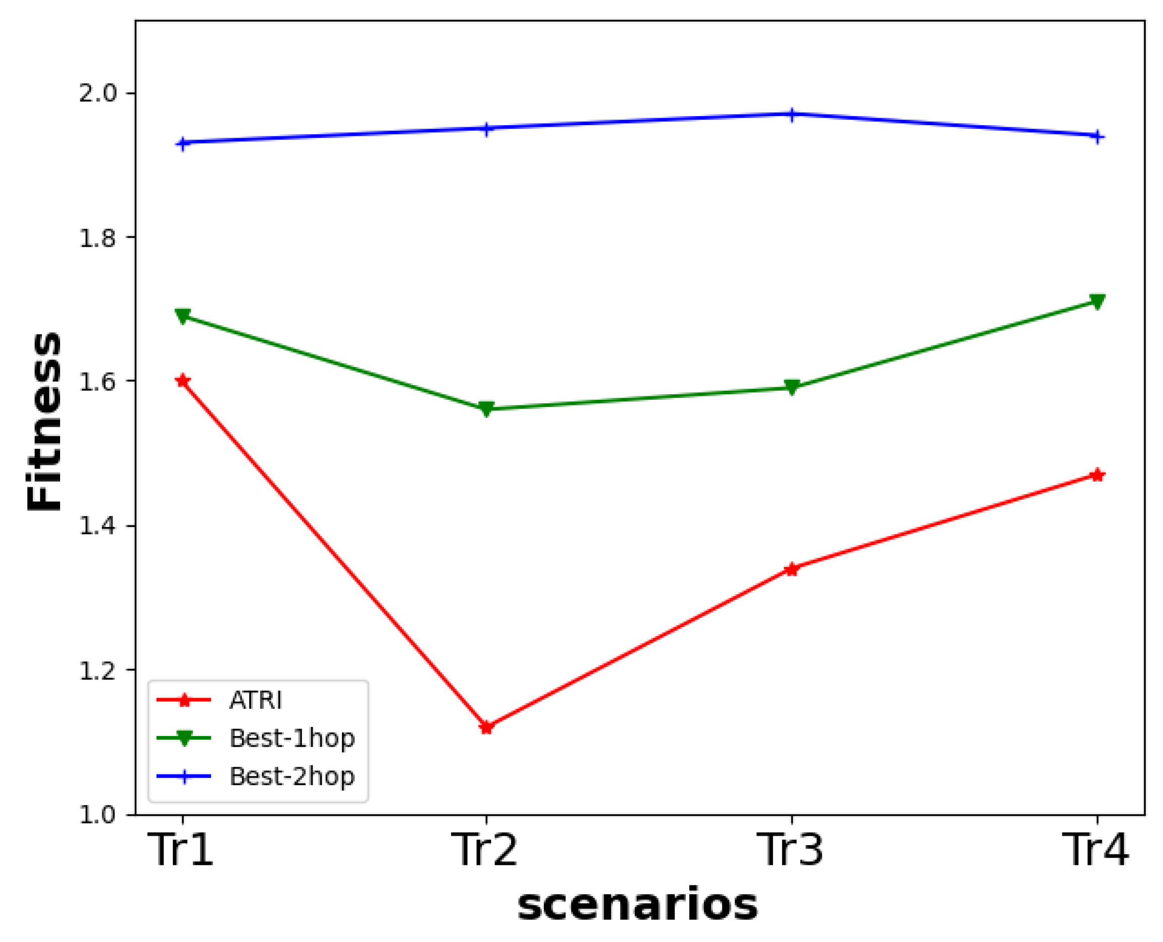
The simulation experiments ran 10 times with different random seeds to evolve solutions considering one-hop and two-hop communication between UAVs. Figure 7 and Table 2 show the fitness obtained using , , and ATRI [15] on the four training scenarios with 156 UAVs and 200 users, where and are the best solutions evolved using GA considering one-hop and two-hop communication respectively. Table 2 shows that, on , the performance is higher than , and higher than ATRI.
In addition, the performance of is higher than ATRI. Similar performance improvements are observed on , , and . On average, the performance is higher than and higher than ATRI. Similarly, the fitness is more than ATRI.
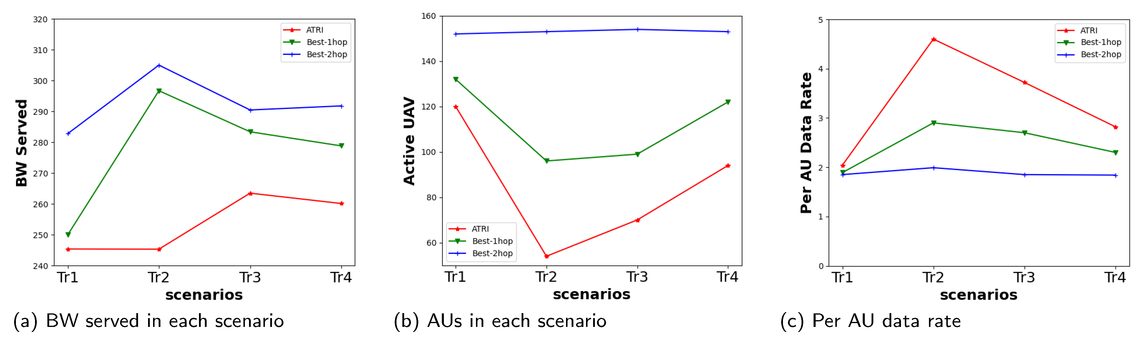
Close inspection indicates that the fitness of is higher because networks deployed using provide more bandwidth coverage to users compared to others and have larger numbers of AUs as shown in Figure 8. Note that fitness is the combination of the percentage bandwidth coverage and percentage of active UAVs. Figure 8 compares (a) the bandwidth served and (b) the number of active UAVs in networks deployed using the , , and ATRI in four scenarios, respectively.
The larger the number of AUs, the smaller the per AU data rate provided to users, leading to less energy consumption and increasing the longevity of the network. Figure 8c shows that the per AU data rate for is smaller than the other two, indicating a higher number of AUs and thus a higher fitness. The figure also shows that the per AU data rate for is smaller than ATRI, again indicating higher fitness than ATRI. These results provide evidence that the proposed genetic-algorithm-optimized network deployment approach is better than ATRI, the current best dynamic network deployment technique. Additional experiments were conducted by considering three-hop communication between UAVs, but no significant performance improvement was observed.
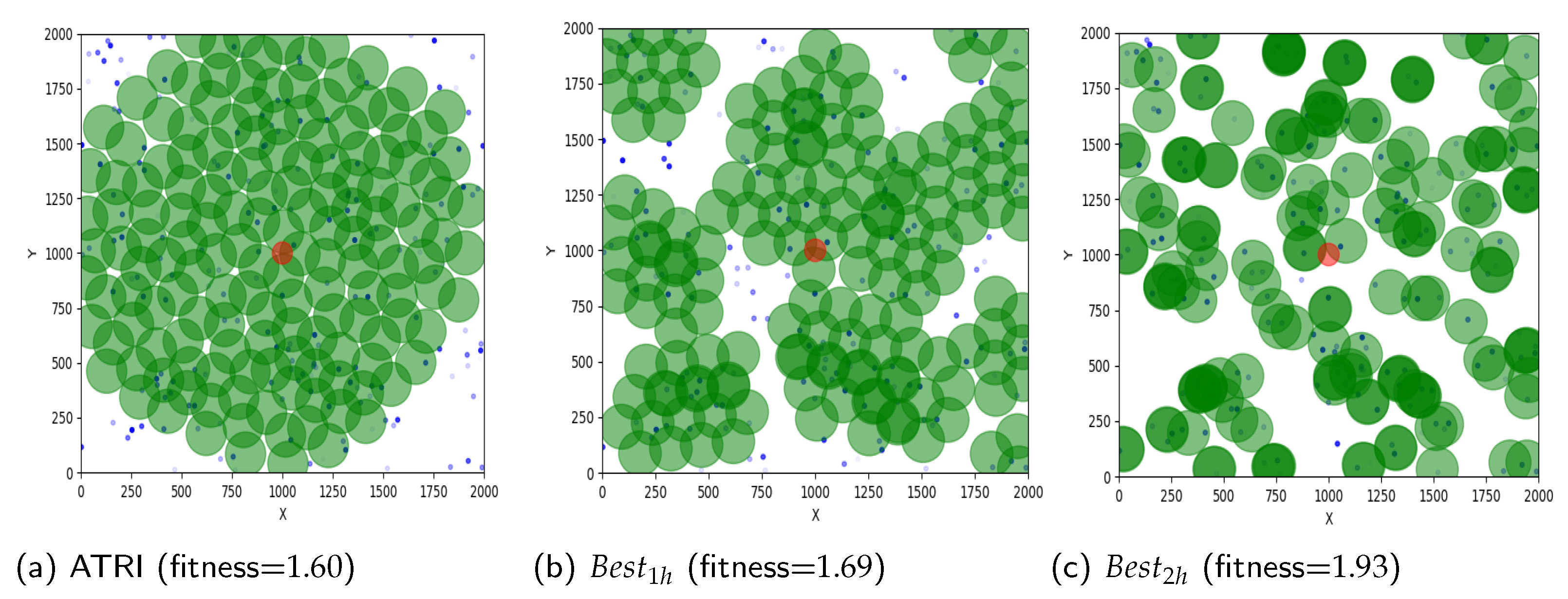
To determine why ATRI’s performance is inferior to GANet, UAVs distributions in the networks deployed using ATRI, , and on the first training scenario () are shown by Figure 9. The figure illustrates that solutions (, ) evolved using GA allow UAVs to move close to users that are distributed throughout the AOI (see Figure 9b,c) while maintaining connectivity with the command center. The evolved potential field parameters guide UAVs toward the area with more user concentration to serve them better. This leads to a higher number of AUs in the deployed network, better network capacity utilization, and higher fitness. However, in the case of ATRI as shown by Figure 9a, the distribution of UAVs does not cover corners, has a circular deployment pattern, and also contains a larger number of IUs (inactive UAVs), resulting in less fitness compared to GANet. It is important to note that ATRI uses one-hop communication for the network deployment, and thus a comparison of ATRI with GANet one-hop is best suited. The next subsection explicitly compares ATRI and GANet one-hop.
6.2.2. GANet-1 hop vs. ATRI
Figure 10 shows networks deployed using ATRI and on the second () and third () training scenarios. In , which has two user clusters, ATRI’s performance is lower than ’s. A similar pattern can be seen for as well. ATRI-deployed UAVs are more uniformly distributed across the AOI, whereas, with GANet, UAVs have learned parameter values that enable them to cluster around users while maintaining connectivity to the command center. This increases the number of AUs (active UAVs) in the network and thus increases the fitness and reduces the per active UAV data rate to users. Note that, on , where users are more uniformly distributed, ATRI’s performance is comparable to GANet. However, in the remaining scenarios, where the users’ distribution is non-uniform, GANet performed better, pointing out the weakness of the ATRI technique over non-uniform users’ distributions.
6.3. Generalizability of Evolved Solutions
Previous subsections have demonstrated that outperforms other solutions when there are 200 users and 156 UAVs. However, the number of users and UAVs can vary depending on situations; thus, in order to find the robustness and generalizability of evolved solutions in different environments, the same set of experiments was conducted using the same evolved solutions (, ) but with varied numbers of users, UAVs, and distributions of users. We changed the number of users and UAVs by at a time (200, 150, 100, and 50 users and 156, 117, and 78 UAVs) and recorded the fitness of each unique pair of UAVs and users. Table 3 and Table 4 compare the fitness obtained with varied numbers of UAVs and users. Based on Table 3, on average, over four scenarios, the performance of is between 17.11–45.94% larger than and ATRI. Similarly, according to Table 4, the fitness is to higher than ATRI, and between 14.46–27.27% more than . We also observed a similar performance improvement pattern between and ATRI, where ’s fitness is higher by to .
These tables show that with changes in either the number of users or both the number of UAVs and users, the performance is still the best, indicating that evolved solutions are robust and generalizable. Figure 11a shows the distribution of fitness for each unique pair of users and UAVs using ATRI, , and on the training scenarios. Here, performed statistically significantly better than both and ATRI with p-value . This provides evidence that, even with a different numbers of users and UAVs, GANet works well in training scenarios.
Similar experiments were conducted on 100 testing scenarios, and the fitness of each unique pair of UAVs and users was recorded on every testing scenario. Figure 11b shows the fitness distribution on 100 testing scenarios, where again the performance of is statistically significant, with a p-value against the other two. These results provide evidence that once GANet optimizes potential field values for a set of UAVs on a set of training scenarios, the performance remains the same on new unseen scenarios with different numbers of users, UAVs, and user distributions.
6.4. Maximizing the Minimum Objective
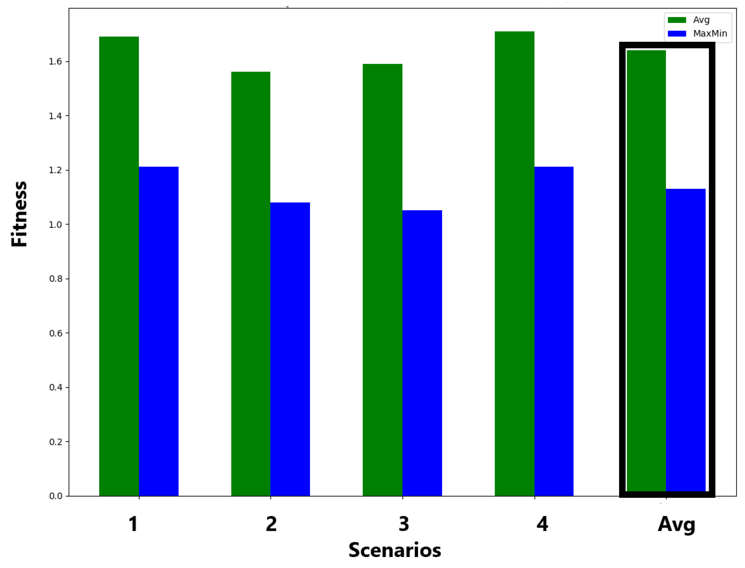
In all previous experiments, the goal was to optimize the fitness score computed as the average performance (Equation (3)) over four training scenarios. Another approach is to maximize the minimum performance [45,46]. However, when comparing the GANet one-hop performance between maximizing the minimum (maximin) and maximizing the average, we found that maximizing the average performs significantly better. Figure 12 shows that the best solution evolved using the averaged fitness, green bar, performed better than the best solution evolved with the maximin fitness, blue bar, on all four scenarios. On average, the averaged fitness performed better than the maximin fitness. We believe that the averaging performance better preserves diversity in the population, leading to more exploration by the genetic algorithm and ultimately resulting in a better performance.
7. Conclusions and Future Work
This paper introduces a unified approach for deploying networks using genetic algorithms optimization. Unlike prior works, the proposed approach unifies the representation across both the search and service phases of network deployment using potential fields. The proposed GANet optimizes potential field parameters that work robustly for different user distributions. In the first phase, the potential field parameters are derived, and, in the second phase, an elitist genetic algorithm optimizes another set of non-linear potential field parameters to maximize the bandwidth while increasing the network longevity.
The results indicate that GANet deployment is significantly better than the current state-of-the-art network deployment algorithm, ATRI. Additionally, the study demonstrates how different levels of information exchange between UAVs affect performance. GANet with two-hop UAV communications outperformed one-hop UAV communication. The experiments show that the offline evolved solutions are robust and work well on 100 never-before-seen test scenarios with different numbers of UAVs and users, providing evidence for the potential-fields-based approach’s robustness and generalizability. GANet adapts better when users are non-uniformly distributed and matches or exceeds ATRI’s performance with more uniform distributions.
In the future, we plan to extend this work by considering dynamic bandwidth requirements for users and maintaining coverage and bandwidth as users move towards the rescue.
Author Contributions
Conceptualization R.D., S.J.L.; methodology, R.D., S.J.L.; formal analysis, R.D.; investigation, R.D.; resources, R.D., S.J.L.; data curation, R.D.; writing—original draft preparation, R.D.; writing—review and editing, R.D., S.J.L.; visualization, R.D.; supervision, S.J.L.; project administration, S.J.L.; funding acquisition, S.J.L. All authors have read and agreed to the published version of the manuscript.
Funding
This material is based upon research supported by, or in part by, the U. S. Office of Naval Research under award number N00014-22-1-2122.
Institutional Review Board Statement
Not applicable.
Informed Consent Statement
Not applicable.
Data Availability Statement
All data used to support the findings of the study is included in this paper.
Conflicts of Interest
The authors declare no conflict of interest.
Abbreviations
The following abbreviations are used in this manuscript:
| GA | Genetic Algorithms |
| GANet | Genetic Adaptive Network Deployment |
| AOI | Area of Interest |
| ATRI | Adaptive Triangulation |
| PF | Potential Field |
| UAV | Unmanned Aerial Vehicle |
| DT | Delaunay Triangulation |
| CPT | Circle Packing Theorem |
References
- Silvagni, M.; Tonoli, A.; Zenerino, E.; Chiaberge, M. Multipurpose UAV for search and rescue operations in mountain avalanche events. Geomat. Nat. Hazards Risk 2017, 8, 18–33. [Google Scholar] [CrossRef] [Green Version]
- Tomic, T.; Schmid, K.; Lutz, P.; Domel, A.; Kassecker, M.; Mair, E.; Grixa, I.L.; Ruess, F.; Suppa, M.; Burschka, D. Toward a Fully Autonomous UAV: Research Platform for Indoor and Outdoor Urban Search and Rescue. IEEE Robot. Autom. Mag. 2012, 19, 46–56. [Google Scholar] [CrossRef] [Green Version]
- Li, X.; Savkin, A.V. Networked Unmanned Aerial Vehicles for Surveillance and Monitoring: A Survey. Future Int. 2021, 13, 174. [Google Scholar] [CrossRef]
- Lee, S.J.; Lee, D.; Kim, H.J. Cargo Transportation Strategy using T3-Multirotor UAV. In Proceedings of the 2019 International Conference on Robotics and Automation (ICRA), Montreal, QC, Canada, 20–24 May 2019; pp. 4168–4173. [Google Scholar] [CrossRef]
- Carrera-Hernández, J.; Levresse, G.; Lacan, P. Is UAV-SfM surveying ready to replace traditional surveying techniques? Int. J. Remote Sens. 2020, 41, 4820–4837. [Google Scholar] [CrossRef]
- Nex, F.; Remondino, F. UAV for 3D mapping applications: A review. Appl. Geomat. 2014, 6, 1–15. [Google Scholar] [CrossRef]
- Erdelj, M.; Król, M.; Natalizio, E. Wireless sensor networks and multi-UAV systems for natural disaster management. Comput. Netw. 2017, 124, 72–86. [Google Scholar] [CrossRef]
- Boursianis, A.D.; Papadopoulou, M.S.; Diamantoulakis, P.; Liopa-Tsakalidi, A.; Barouchas, P.; Salahas, G.; Karagiannidis, G.; Wan, S.; Goudos, S.K. Internet of things (IoT) and agricultural unmanned aerial vehicles (UAVs) in smart farming: A comprehensive review. Int. Things 2020, 18, 100187. [Google Scholar] [CrossRef]
- Motlagh, N.H.; Bagaa, M.; Taleb, T. UAV-Based IoT Platform: A Crowd Surveillance Use Case. IEEE Commun. Mag. 2017, 55, 128–134. [Google Scholar] [CrossRef] [Green Version]
- Gáspár, Z.; Tarnai, T. Upper bound of density for packing of equal circles in special domains in the plane. Period. Polytech. Civ. Eng. 2000, 44, 13–32. [Google Scholar]
- Chevet, T.; Maniu, C.S.; Vlad, C.; Zhang, Y. Voronoi-based UAVs formation deployment and reconfiguration using MPC techniques. In Proceedings of the IEEE International Conference on Unmanned Aircraft Systems (ICUAS), Dallas, TX, USA, 12–15 June 2018; pp. 9–14. [Google Scholar]
- Mozaffari, M.; Saad, W.; Bennis, M.; Nam, Y.H.; Debbah, M. A tutorial on UAVs for wireless networks: Applications, challenges, and open problems. IEEE Commun. Surv. Tutor. 2019, 21, 2334–2360. [Google Scholar] [CrossRef] [Green Version]
- Dubey, R.; Louis, S.J.; Sengupta, S. Evolving Dynamically Reconfiguring UAV-hosted Mesh Networks. In Proceedings of the 2020 IEEE Congress on Evolutionary Computation (CEC), Glasgow, UK, 19–24 July 2020; pp. 1–8. [Google Scholar] [CrossRef]
- Dubey, R.; Ghantous, J.; Louis, S.; Liu, S. Evolutionary Multi-objective Optimization of Real-Time Strategy Micro. In Proceedings of the 2018 IEEE Conference on Computational Intelligence and Games (CIG), Maastricht, The Netherlands, 14–17 August 2018; pp. 1–8. [Google Scholar]
- Ma, M.; Yang, Y. Adaptive triangular deployment algorithm for unattended mobile sensor networks. IEEE Trans. Comput. 2007, 56, 847–946. [Google Scholar] [CrossRef]
- Binh, L.H.; Truong, T.K. An efficient method for solving router placement problem in wireless mesh networks using multi-verse optimizer algorithm. Sensors 2022, 22, 5494. [Google Scholar] [CrossRef] [PubMed]
- Wang, J.; Jiang, C.; Han, Z.; Ren, Y.; Maunder, R.G.; Hanzo, L. Taking drones to the next level: Cooperative distributed unmanned-aerial-vehicular networks for small and mini drones. IEEE Veh. Technol. Mag. 2017, 12, 73–82. [Google Scholar] [CrossRef] [Green Version]
- Lam, M.L.; Liu, Y.H. Heterogeneous Sensor Network Deployment Using Circle Packings. In Proceedings of the 2007 IEEE International Conference on Robotics and Automation, Rome, Italy, 10–14 April 2007; pp. 4442–4447. [Google Scholar]
- Lyu, J.; Zeng, Y.; Zhang, R.; Lim, T.J. Placement optimization of UAV-mounted mobile base stations. IEEE Commun. Lett. 2016, 21, 604–607. [Google Scholar] [CrossRef] [Green Version]
- Mozaffari, M.; Saad, W.; Bennis, M.; Debbah, M. Efficient deployment of multiple unmanned aerial vehicles for optimal wireless coverage. IEEE Commun. Lett. 2016, 20, 1647–1650. [Google Scholar] [CrossRef]
- Bartolini, N.; Calamoneri, T.; La Porta, T.F.; Silvestri, S. Autonomous deployment of heterogeneous mobile sensors. IEEE Trans. Mob. Comput. 2010, 10, 753–766. [Google Scholar] [CrossRef] [Green Version]
- Patra, A.N.; Regis, P.A.; Sengupta, S. Distributed allocation and dynamic reassignment of channels in UAV networks for wireless coverage. Pervasive Mob. Comput. 2019, 54, 58–70. [Google Scholar] [CrossRef]
- Khatib, O. Real-Time Obstacle Avoidance for Manipulators and Mobile Robots. Int. J. Robot. Res. 1986, 5, 90–98. [Google Scholar] [CrossRef]
- Woods, A.C.; La, H.M. A novel potential field controller for use on aerial robots. IEEE Trans. Syst. Man Cybern. Syst. 2017, 49, 665–676. [Google Scholar] [CrossRef] [Green Version]
- Dubey, R.; Louis, S.; Gajurel, A.; Liu, S. Comparing Three Approaches to Micro in RTS Games. In Proceedings of the 2019 IEEE Congress on Evolutionary Computation (CEC), Wellington, New Zealand, 10–13 June 2019; pp. 777–784. [Google Scholar]
- Howard, A.; Matarić, M.J.; Sukhatme, G.S. Mobile Sensor Network Deployment Using Potential Fields: A Distributed, Scalable Solution to the Area Coverage Problem; Springer: Berlin/Heidelberg, Germany, 2002; pp. 299–308. [Google Scholar]
- Poduri, S.; Sukhatme, G.S. Constrained coverage for mobile sensor networks. In Proceedings of the IEEE International Conference on Robotics and Automation, ICRA’04, New Orleans, LA, USA, 26 April–1 May 2004; Volume 1, pp. 165–171. [Google Scholar]
- Zhao, H.; Wang, H.; Wu, W.; Wei, J. Deployment algorithms for uav airborne networks toward on-demand coverage. IEEE J. Sel. Areas Commun. 2018, 36, 2015–2031. [Google Scholar] [CrossRef]
- Anbalagan, S.; Bashir, A.K.; Raja, G.; Dhanasekaran, P.; Vijayaraghavan, G.; Tariq, U.; Guizani, M. Machine-learning-based efficient and secure RSU placement mechanism for software-defined-IoV. IEEE Internet Things J. 2021, 8, 13950–13957. [Google Scholar] [CrossRef]
- Reina, D.; Tawfik, H.; Toral, S. Multi-subpopulation evolutionary algorithms for coverage deployment of UAV-networks. Ad Hoc Netw. 2018, 68, 16–32. [Google Scholar]
- Deif, D.S.; Gadallah, Y. Wireless Sensor Network Deployment Using A Variable-Length Genetic Algorithm. In Proceedings of the 2014 IEEE Wireless Communications and Networking Conference (WCNC), Istanbul, Turkey, 6–9 April 2014; pp. 2450–2455. [Google Scholar] [CrossRef]
- Harizan, S.; Kuila, P. Coverage and connectivity aware energy efficient scheduling in target based wireless sensor networks: An improved genetic algorithm based approach. Wirel. Netw. 2019, 25, 1995–2011. [Google Scholar]
- Ruetten, L.; Regis, P.A.; Feil-Seifer, D.; Sengupta, S. Area-optimized UAV swarm network for search and rescue operations. In Proceedings of the 2020 10th Annual Computing and Communication Workshop and Conference (CCWC), Las Vegas, NV, USA, 6–8 January 2020; pp. 613–618. [Google Scholar]
- Ab Aziz, N.A.B.; Mohemmed, A.W.; Alias, M.Y. A wireless sensor network coverage optimization algorithm based on particle swarm optimization and Voronoi diagram. In Proceedings of the 2009 International Conference on Networking, Sensing and Control, Okayama, Japan, 26–29 March 2009; pp. 602–607. [Google Scholar]
- Li, J.; Lu, D.; Zhang, G.; Tian, J.; Pang, Y. Post-disaster unmanned aerial vehicle base station deployment method based on artificial bee colony algorithm. IEEE Access 2019, 7, 168327–168336. [Google Scholar]
- Abdulrab, H.Q.; Hussin, F.A.; Abd Aziz, A.; Awang, A.; Ismail, I.; Saat, M.S.M.; Shutari, H. Optimal coverage and connectivity in industrial wireless mesh networks based on Harris’ hawk optimization algorithm. IEEE Access 2022, 10, 51048–51061. [Google Scholar]
- Patra, A.N.; Regis, P.A.; Sengupta, S. Dynamic self-reconfiguration of unmanned aerial vehicles to serve overloaded hotspot cells. Comput. Electr. Eng. 2019, 75, 77–89. [Google Scholar]
- Deb, K.; Pratap, A.; Agarwal, S.; Meyarivan, T. A fast and elitist multiobjective genetic algorithm: NSGA-II. IEEE Trans. Evol. Comput. 2002, 6, 182–197. [Google Scholar]
- Tian, X.; Guo, Y.; Negenborn, R.R.; Wei, L.; Lin, N.M.; Maestre, J.M. Multi-scenario model predictive control based on genetic algorithms for level regulation of open water systems under ensemble forecasts. Water Resour. Manag. 2019, 33, 3025–3040. [Google Scholar]
- Louis, S.J.; Liu, S. Multi-objective evolution for 3D RTS micro. In Proceedings of the 2018 IEEE Congress on Evolutionary Computation (CEC), Rio de Janeiro, Brazil, 8–13 July 2018; pp. 1–8. [Google Scholar]
- Liu, S.; Louis, S.; Ballinger, C. Evolving Effective Micro Behaviors in Real-Time Strategy Games. IEEE Trans. Comput. Intell. Games 2016, 8, 351–362. [Google Scholar] [CrossRef]
- Dubey, R.; Louis, S.J. Evolving potential field parameters for deploying UAV-based two-hop wireless mesh networks. In Proceedings of the Genetic and Evolutionary Computation Conference Companion (GECCO 21), Lille, France, 10–14 July 2021; pp. 311–312. [Google Scholar]
- Unity3D. Available online: https://unity.com/ (accessed on 25 March 2023).
- OpenMPI. Available online: ttps://www.open-mpi.org/ (accessed on 25 March 2023).
- Wang, H.; Feng, L.; Jin, Y.; Doherty, J. Surrogate-assisted evolutionary multitasking for expensive minimax optimization in multiple scenarios. IEEE Comput. Intell. Mag. 2021, 16, 34–48. [Google Scholar] [CrossRef]
- Pióro, M.; Żotkiewicz, M.; Staehle, B.; Staehle, D.; Yuan, D. On max–min fair flow optimization in wireless mesh networks. Ad Hoc Netw. 2014, 13, 134–152. [Google Scholar] [CrossRef] [Green Version]
Figure 1.
Four training scenarios, where blue dots show the location of users. Lighter color represents low-bandwidth-demanding users and darker color shows higher bandwidth demand.
Figure 1.
Four training scenarios, where blue dots show the location of users. Lighter color represents low-bandwidth-demanding users and darker color shows higher bandwidth demand.

Figure 2.
The figures show three testing scenarios (, and ). The robustness of the best-evolved solution will be tested in these scenarios.
Figure 2.
The figures show three testing scenarios (, and ). The robustness of the best-evolved solution will be tested in these scenarios.

Figure 3.
UAVs moving under the influence of potential fields with parameters () as (1, 1, , −2) to create a network with zero coverage gap.
Figure 3.
UAVs moving under the influence of potential fields with parameters () as (1, 1, , −2) to create a network with zero coverage gap.

Figure 4.
Deployment of UAVs at the end of the first phase on the third training scenario. Blue dots represent users, green circles represent UAVs’ coverage areas, and the red circle represents the location of the command center. A black circle shows an inactive UAV and the magenta circle shows an inactive UAV.

Figure 5.
The figure shows five UAVs with blue-colored regions representing UAV’s ground coverage and five users represented by light yellow-colored dots. Red and black arrows show directions of and . Kth UAV has two users within its ( = 2): three one-hop ( = 3) and one two-hop ( = 1) neighbors. In this example, = 0 and = 0.

Figure 6.
UAV deployment within an AOI with 10 users (blue dots). (a) shows initial UAV positions covering the area, (b) shows the final UAV positions focusing on user locations and bandwidth sharing, and (c) compares the three search algorithms.
Figure 6.
UAV deployment within an AOI with 10 users (blue dots). (a) shows initial UAV positions covering the area, (b) shows the final UAV positions focusing on user locations and bandwidth sharing, and (c) compares the three search algorithms.

Figure 7.
Comparing the best fitness obtained using GANet 1-hop, GANet 2-hop, and ATRI.

Figure 8.
Comparing results on four training scenarios: (a) bandwidth served by deployed networks, (b) the number of AUs in the networks, and (c) per AU data rate.
Figure 8.
Comparing results on four training scenarios: (a) bandwidth served by deployed networks, (b) the number of AUs in the networks, and (c) per AU data rate.

Figure 9.
(a–c) show networks on using ATRI, GANet 1-hop, GANet 2-hop. GANet obtains better performance by focusing more on areas with users and avoiding areas with no users.
Figure 9.
(a–c) show networks on using ATRI, GANet 1-hop, GANet 2-hop. GANet obtains better performance by focusing more on areas with users and avoiding areas with no users.

Figure 10.
Network deployments of and ATRI on and . In both scenarios, performed better than ATRI because GANet allows UAVs to move toward users with bandwidth demand.
Figure 10.
Network deployments of and ATRI on and . In both scenarios, performed better than ATRI because GANet allows UAVs to move toward users with bandwidth demand.

Figure 11.
(a,b) show the distribution of fitness for each unique pair of UAVs and users on 4 training and 100 testing scenarios, respectively. In each case, better indicates better transferability of evolved solutions.
Figure 11.
(a,b) show the distribution of fitness for each unique pair of UAVs and users on 4 training and 100 testing scenarios, respectively. In each case, better indicates better transferability of evolved solutions.

Figure 12.
GANet performance when maximizing the average performance across four training scenarios (green) compared to maximizing the minimum performance over four (blue).
Figure 12.
GANet performance when maximizing the average performance across four training scenarios (green) compared to maximizing the minimum performance over four (blue).


Table 1.
Comparison of wireless network deployment methods.
| Papers | Methods | Network | Control | User Distribution | Generalizable |
|---|---|---|---|---|---|
| Static (S) | Centralized (CC) | Uniform (U) | |||
| Dynamic (D) | Distributed (DC) | Non-Uniform (NU) | |||
| [10] | CPT | S | DC | U, NU | No |
| [11] | VD | S | DC | U, NU | No |
| [15] | ATRI | D | DC | U, NU | No |
| [18] | CPT | S | CC | U, NU | No |
| [19] | CPT | D | CC | U | No |
| [20] | CPT | D | CC | U | No |
| [21] | VD | D | DC | U | No |
| [22] | DT | D | DC | U | No |
| [26] | PF | S | DC | U, NU | Yes |
| [27] | PF | S | DC | U, NU | Yes |
| [28] | PF | D | DC | U, NU | No |
| [30] | GA | S | CC | U, NU | No |
| [31] | GA | S | CC | U, NU | No |
| [32] | GA | S | CC | U, NU | No |
| [33] | GA | S | CC | U | No |
| [34] | PSO | S | CC | U, NU | No |
| [35] | ABC | S | CC | U, NU | No |
| [36] | HHO | S | CC | U | No |
| proposed | GA and PF | D | DC | U, NU | Yes |
Table 2.
Comparing fitness obtained with 156 UAVs and 200 users on training scenarios.
| Users | Methods | ||||
|---|---|---|---|---|---|
| ATRI | 1.60 | 1.12 | 1.34 | 1.47 | |
| 200 | GANet-1 hop | 1.69 | 1.56 | 1.59 | 1.71 |
| GANet-2 hop | 1.93 | 1.95 | 1.97 | 1.94 |
Table 3.
Comparing fitness with different numbers of UAVs and 200 users on training scenarios.
| Users | Methods | ||||||||
|---|---|---|---|---|---|---|---|---|---|
| 117 UAVs | 78 UAVs | ||||||||
| ATRI | 1.50 | 1.02 | 1.29 | 1.40 | 1.32 | 0.76 | 1.13 | 1.26 | |
| 200 | GANet-1 hop | 1.52 | 1.53 | 1.61 | 1.62 | 1.47 | 1.25 | 0.98 | 1.57 |
| GANet-2 hop | 1.64 | 1.88 | 1.90 | 1.84 | 1.65 | 1.53 | 1.59 | 1.69 | |
Table 4.
Comparing fitness with different numbers of UAVs and users on training scenarios.
| Users | Methods | ||||||||||||
|---|---|---|---|---|---|---|---|---|---|---|---|---|---|
| 156 UAVs | 117 UAVs | 78 UAVs | |||||||||||
| ATRI | 1.52 | 1.11 | 1.29 | 1.43 | 1.38 | 1.09 | 1.28 | 1.33 | 1.20 | 0.71 | 1.14 | 1.28 | |
| 150 | GANet-1 hop | 1.58 | 1.44 | 1.53 | 1.62 | 1.52 | 1.52 | 1.62 | 1.71 | 1.36 | 1.38 | 0.93 | 1.60 |
| GANet-2 hop | 1.97 | 1.96 | 1.95 | 1.93 | 1.69 | 1.88 | 1.80 | 1.91 | 1.63 | 1.66 | 1.64 | 1.66 | |
| ATRI | 1.34 | 1.13 | 1.24 | 1.42 | 1.26 | 1.40 | 1.28 | 1.34 | 1.10 | 0.81 | 0.93 | 1.23 | |
| 100 | GANet-1 hop | 1.58 | 1.29 | 1.39 | 1.55 | 1.42 | 1.33 | 1.48 | 1.57 | 1.24 | 1.31 | 1.50 | 1.58 |
| GANet-2 hop | 1.84 | 1.98 | 1.93 | 1.98 | 1.78 | 1.86 | 1.78 | 1.91 | 1.61 | 1.49 | 1.66 | 1.78 | |
| ATRI | 1.18 | 1.13 | 1.16 | 1.20 | 1.05 | 1.06 | 1.12 | 1.06 | 0.81 | 0.37 | 0.71 | 0.84 | |
| 50 | GANet-1 hop | 1.23 | 1.20 | 1.29 | 1.38 | 1.22 | 1.27 | 1.36 | 1.25 | 1.08 | 1.34 | 1.27 | 1.15 |
| GANet-2 hop | 1.32 | 1.92 | 1.29 | 1.64 | 1.51 | 1.77 | 1.85 | 1.60 | 1.21 | 1.70 | 1.67 | 1.55 | |
Disclaimer/Publisher’s Note: The statements, opinions and data contained in all publications are solely those of the individual author(s) and contributor(s) and not of MDPI and/or the editor(s). MDPI and/or the editor(s) disclaim responsibility for any injury to people or property resulting from any ideas, methods, instructions or products referred to in the content. |
© 2023 by the authors. Licensee MDPI, Basel, Switzerland. This article is an open access article distributed under the terms and conditions of the Creative Commons Attribution (CC BY) license (https://creativecommons.org/licenses/by/4.0/).
Share and Cite
MDPI and ACS Style
Dubey, R.; Louis, S.J. Genetic Algorithms Optimized Adaptive Wireless Network Deployment. Appl. Sci. 2023, 13, 4858. https://0-doi-org.brum.beds.ac.uk/10.3390/app13084858
AMA Style
Dubey R, Louis SJ. Genetic Algorithms Optimized Adaptive Wireless Network Deployment. Applied Sciences. 2023; 13(8):4858. https://0-doi-org.brum.beds.ac.uk/10.3390/app13084858
Chicago/Turabian StyleDubey, Rahul, and Sushil J. Louis. 2023. "Genetic Algorithms Optimized Adaptive Wireless Network Deployment" Applied Sciences 13, no. 8: 4858. https://0-doi-org.brum.beds.ac.uk/10.3390/app13084858
Note that from the first issue of 2016, this journal uses article numbers instead of page numbers. See further details here.