
Effects of “S”-Type Bowed Guide Vanes on Unsteady Flow in 1.5-Stage Axial Compressors
1
State Key Laboratory of Strength and Vibration of Mechanical Structures, School of Energy and Power Engineering, Xi’an Jiaotong University, Xi’an 710049, China
2
MOE Key Laboratory of Thermo-Fluid Science and Engineering, School of Energy and Power Engineering, Xi’an Jiaotong University, Xi’an 710049, China
*
Author to whom correspondence should be addressed.
Appl. Sci. 2023, 13(8), 5071; https://0-doi-org.brum.beds.ac.uk/10.3390/app13085071
Submission received: 1 April 2023
/
Revised: 15 April 2023
/
Accepted: 17 April 2023
/
Published: 18 April 2023
(This article belongs to the Topic Fluid Mechanics)
Abstract
:In axial compressors, the unsteady flow caused by the interaction between dynamic and static cascades will make the moving vanes subject to periodic forces and increase the risk of high-cycle fatigue fractures. In this study, an “S”-type bowed guide vane was designed and a 1.5-stage axial compressor model was established. For five guide vanes with different bending coefficients, unsteady numerical simulation was carried out under design conditions and near-blockage conditions. The influence of the guide vane bending coefficient on the pressure ratio and efficiency is analyzed, and the aerodynamic exciting force on moving vanes is analyzed by using the fast Fourier transform. The study shows that the model with an “S”-type bowed guide vane can greatly reduce the amplitude of aerodynamic exciting force on moving vanes. The model with a guide vane bending coefficient of −10 mm can reduce the tangential and axial aerodynamic exciting force amplitudes at the first-order blade-passing frequency by 90.82% and 90.39% under the design conditions, respectively. Under the near-blockage condition, the tangential and axial aerodynamic exciting force amplitudes can be reduced by 85.84% and 86.58%, respectively. This can greatly improve the vibration safety of the moving vane.
1. Introduction
The unsteady flow caused by the relative motion between the moving and static vanes is an intrinsic unsteady phenomenon in fluid machinery, and has certain periodic laws. The outlet aerodynamic parameters of the upstream vane are not uniform, but show a periodic distribution [1], so the downstream moving vane will bear the high-frequency periodic aerodynamic exciting force during rotation. For axial flow compressors, the high-frequency aerodynamic exciting force on the moving vane will increase the high-cycle fatigue fracture risk and reduce the compressor service life. It is also an important part of the compressor aerodynamic noise. Therefore, it is very important to study the unsteady flow phenomena in axial flow compressors and explore efficient measures to reduce the flow exciting force of moving vanes for safe and stable operations [2].
Many scholars have carried out detailed research on unsteady flow in axial flow compressors. Gallus et al. [3,4] experimentally measured the pressure fluctuation on the surface of the moving and stator blades in the subsonic compressor as well as the shape of the moving wake. The results show that the higher-order harmonics of potential flow interaction attenuate very quickly. In most cases, the amplitude of the second harmonic is only 20% to 40% of the first harmonic, and the influence of the higher harmonic on the blade vibration is very small. When the axial clearance of the cascade row is small, the potential flow interference and the wake maintain the same order of magnitude. Thus, increasing the axial clearance can reduce the discrete tone level. The research by Gorrell [5] shows that, in transonic compressors, with a smaller axial clearance between moving and stator blades, the aerodynamic loss caused by stator–rotor interactions increases gradually, resulting in the decline of axial compressor performance. Douglas et al. [6] studied the unsteady flow characteristics generated by the interaction between guide vane wakes and moving blades of axial compressors through experiments, and analyzed the probability distribution of the wake characteristics. The results indicate that the relative position between the moving and stator blades have a strong correlation with unsteady aerodynamic response of the moving vanes, but this correlation would be weakened with the decrease of the flow rate under working conditions. Burkhardt et al. [7] conducted the unsteady measurements of the moving and stator blades for the high load 1.5-stage axial compressor and studied the influence of different working conditions on boundary layer transition. Smith et al. [8] explored the influence of the interaction between upstream blades on the downstream blade boundary layer transition position through a 3-stage axial compressor test rig.
The research on unsteady aerodynamic exciting forces can be traced back to the 1960s. Lefcort [9] used a simple analysis model to predict the pressure fluctuation of adjacent blades. However, due to the lack of cognition at that time, the author could only make rough assumptions about the research model, which pose a limitation on its adaptability. Daigji et al. [10] studied the correlation between wake and unsteady aerodynamic forces, and the influence of wake on moving cascades is studied through the combination of the finite element method and the finite difference method. Mailach et al. [11] studied the influence mechanism of unsteady blade row interference on unsteady aerodynamic forces of a 4-stage compressor. In this research, the time and frequency domain distribution of aerodynamic forces are analyzed. It is pointed out that the amplitude and shape of aerodynamic forces are not only related to the wake strength and flow field potential, but also affected by the interaction between the wake and the potential flow field. Smith et al. [12] set up a three-stage axial compressor test platform and used high-frequency response pressure sensors to conduct tests. The results show that the rotor wake and tip clearance flow are the main reasons for the unsteady load fluctuation of the downstream stator blades. The two rows of moving vanes adjacent to the stator blade have a significant effect on the unsteady pressure fluctuation on its surface, and the timing effect has obvious effects on the dynamic–static interference.
It can be found that the unsteady flow in the compressor is mainly caused by the interference of the potential flow field and wake. The stator–rotor interaction plays a decisive role in the unsteady force on the blade. Many scholars have designed the structure of the blade in an effort to improve the unsteady aerodynamic performance as well as reduce the aerodynamic exciting force and noise. Monk et al. [13] analyzed the effect of asymmetric stator distribution on unsteady flow by researching a three-stage compressor. It can be found from Fourier transform results that the number of stator blades is asymmetric, which reduces the amplitude of aerodynamic excitation and deflects the excitation frequency. Wenjie et al. [14] studied the method of reducing the dynamic and static interference noise using nonuniform trailing edge blowing. Through numerical simulation, they found that the axial force amplitude of the moving vane at the first-order blade-passing frequency can be reduced by 63.83%. Milidonis et al. [15] studied the effects of clocking on acoustic noise-generation characteristics in a 1.5-stage axial compressor using high-fidelity and low-order numerical methods. It is found that stator clocking has little effect on compressor efficiency and tonal acoustic noise levels in the far field but the amplitude varies differently when the clocking position varies in the near field. Asymmetric stator distribution and nonuniform trailing edge blowing can play a better role in reducing the amplitude of the airflow exciting force. However, the structure of these designs is very complex and the cost is greatly increased.
Improving unsteady performance by changing the vane stacking in space is also a research direction. Weir et al. [16] measured the influence of forward swept rotors and inclined guide vane on rotor–stator interaction noise. The results show that the noise of the improved fan model is lower than that of the original model in most conditions. Bamberger et al. [17] changed the sweep strategy and geometrical parameters to optimize the sound emission and efficiency of a low-pressure axial fan using the simplex method, and verified it via experiments and numerical methods. Bohn et al. [18] compared the 3D unsteady flow field of a cylindrical-designed blade and bow-blade with numerical calculations, and found that bow-blades can reduce the wake intensity and the unsteady profile pressure fluctuations. Laborderie et al. [19] established a two-stagger-angle method to predict the vane camber effects on fan noise. It has been shown that the interaction noise sources are predominant in the leading-edge region. Ling et al. [20] optimized the stacking line of the compressor curved vane of a linear compressor, analyzed the influence of a stack line on aerodynamic loss, and obtained the optimum stack line under different geometric parameters and aerodynamic conditions. Rajesh et al. [21] proposed a variable camber inlet guide to increase the stable operating range of a low-speed axial compressor and analyzed its stable operating range and efficiency at an off-design point using numerical simulation. Wadia et al. [22] designed a swept and leaned-outlet guide vane. Through numerical calculation, it is found that it can reduce the potential flow interaction of stators and rotors and reduce the back-pressure disturbance. Keke et al. [23] studied the influence of a stator blade camber on the unsteady performance of axial turbines, and found that a bowed stator can effectively reduce the airflow exciting force amplitude of rotor blades. Xiangyi et al. [24] studied the effect of variable-camber inlet guide vanes on the performance of compressors using a numerical method. Results show that the stall margin and the total pressure rise of the compressor rotor are sensitive to the span range of the variable-camber. Lei et al. [25] studied the effect of bowed outlet guide vanes in gas turbines on the heat conduction and aerodynamic performance near the endwall using numerical simulations. It was found that the bowed vanes can effectively reduce the endwall heat transfer. Niu et al. [26] found that forward-swept and positive-leaned vanes can reduce the exciting force and make the output power more stable for gas turbines using numerical calculations. Liu et al. [27] conducted numerical and aeroacoustic studies on axial flow compressors with different lean angles of the stator, and found that a positive leaned stator has better noise reduction effect than the negative. Zhu et al. [28] found that the combination of blade lean and blade clocking can improve unsteady aerodynamic performance and adiabatic efficiency through the numerical simulation of 1.5-stage axial turbines.
Through the above research, it can be found that most of the researches are aimed at improving unsteady aerodynamic performance or reducing aerodynamic noise. However, in order to ensure the safe and stable operation of the compressor, the unsteady force on the vane is also very important. In addition, changing the vane stacking line in the tangential direction has a greater impact on the unsteady aerodynamic performance of fluid machinery, and the effect of reducing unsteady aerodynamic force is more obvious. However, most of the designs are leaned vanes and “C”-type bowed vanes. This study improved the structure of the guide vane of the axial compressor with an “S”-type bowed guide vane, and the improvement is validated on a 1.5-stage axial compressor model. For five guide vane models with different bending coefficients, the unsteady numerical simulation was carried out under design conditions and near-blockage conditions, respectively. The influence of the “S”-type bowed guide vane on the aerodynamic performance and the aerodynamic exciting force on moving vanes are both studied to explore the optimal structure of the guide vane of the 1.5-stage axial compressor.
2. Methods
2.1. The 1.5-Stage Axial Compressor with the “S”-Type Bowed Guide Vane
In this study, based on a civil axial compressor, a numerical calculation model of a 1.5-stage full three-dimensional axial compressor including a guide vane, moving vane, and stator vane was established. The structural parameters of the compressor model are shown in Table 1.
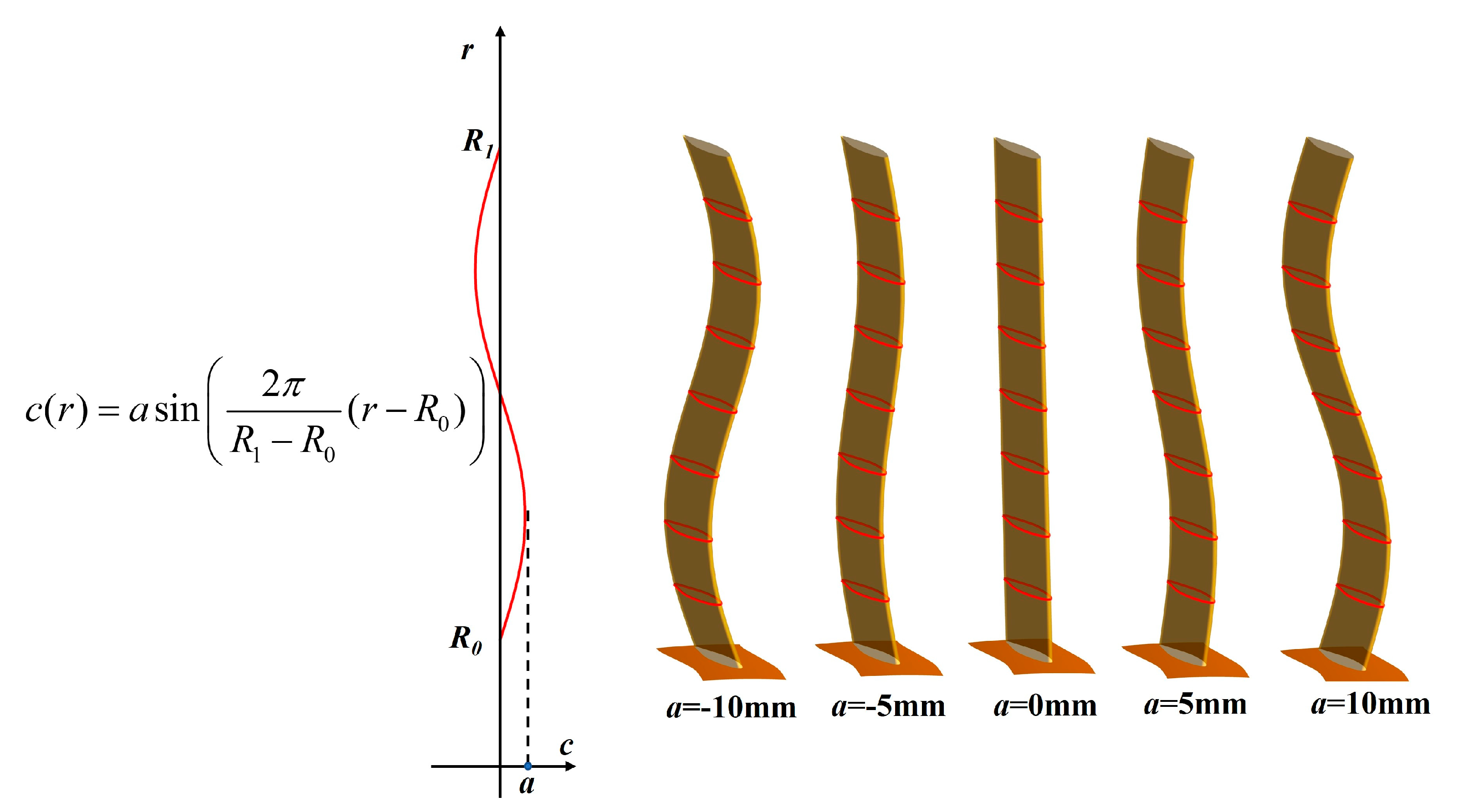
The guide vane of the original model is straight. We fix the endwall sections and ensure that the profiles at different blade height positions are the same. The stacking line is bent into the “S”-type in the form of a sine function in the tangential direction and its position in the axial direction is unchanged. The stacking line of the “S”-type bowed curved guide vane can be expressed as shown in Equation (1) in the cylindrical coordinate system:
where is defined as the guide vane bending coefficient, which represents the maximum distance of the “S”-type bowed guide vane from the original vane in the tangential direction. R1 is the outer diameter of the guide vane, R0 is the inner diameter of the guide vane, r is the radial coordinate of the stacking line, and c is the tangential coordinate of the stacking line. Figure 1 shows the guide vanes with different bending coefficients.
In this study, the 1.5-stage axial compressor with different bending coefficient is numerically simulated under the design condition and near-blockage condition, respectively. The boundary conditions of the two working conditions are shown in Table 2.
2.2. Numerical Method
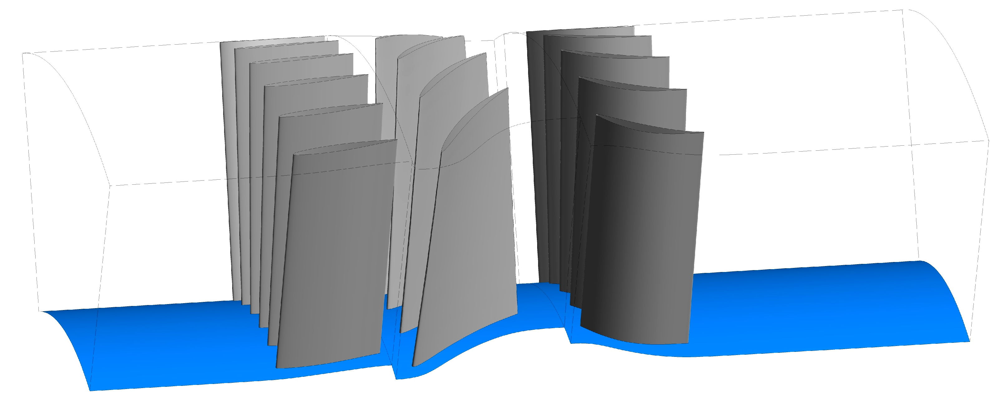
The full three-dimensional unsteady Navier–Stokes equations are used for numerical calculation, while real air is used as the working medium. The SST k-ω turbulence model is selected for unsteady aerodynamic analysis in this study. The computational domain of aerodynamic analysis is established with the number of guide vanes, moving vanes, and stator vanes being 6, 4, and 5, respectively. The computational domain is one-ninth of the whole axial compressor model. The computational domains extend two times of the guide vane chord ahead of the guide vane and three times of the stator chord length behind the stator vane to improve the computational accuracy. Taking the = 0 mm model as an example, the geometric model of the aerodynamic computational domain is shown in Figure 2.
The numerical analysis is completed using the ANSYS CFX 16.0 software. The transient rotor stator method [29,30] is adopted for dynamic and static interfaces. The transient rotor stator method can well simulate the relative motion between the guide vane and the moving vane as well as the relative motion between the moving vane and the stator vane by using a sliding interface. The relative position of the grids on each side of the interface is updated each timestep with the rotation of the moving vane. A high accuracy difference scheme is adopted for convection terms and a second-order upwind scheme is adopted for time-term discretization. The inlet turbulence intensity is 5% for a fully developed flow. The time step equals 7.668 × 10⁻⁶ s, which means it takes 30-time steps for a moving vane to sweep through a guide vane. In the unsteady calculation, the axial force and the tangential force of a single moving vane are detected. When there are more than 10 regular cycles, the calculation is considered to be convergent.
The frequency-domain distribution of unsteady aerodynamic exciting forces is obtained using fast Fourier transform, and the frequency-domain distribution law of unsteady aerodynamic forces can be obtained, including excitation amplitude and excitation frequency, so as to further reveal the mechanism of aerodynamic excitation. In this study, the function with a period of 2π is used to express the unsteady force of the moving vane, as shown in Equation (2) [23].
The spectrum function can be obtained using Fourier transformation of Equation (1), as shown in Equation (3) [23].
For the overall quantities, we validated the numerical calculation method through the numerical analysis of NASA Rotor 67. Strazisar et al. [31] gave detailed test measurement values of the blade. For the blade of Rotor 67, the number of grid nodes of the single channel numerical model is 0.921 million, and the number of elements is 0.854 million. The grid is densified at the tip clearance and the blade surface. Parameter settings for numerical analysis are as follows: (1) The calculation domain is set as the rotation domain, the rotational speed is 16,043 rpm, and the working medium is ideal gas. The turbulence model is SST k-ω; (2) The total inlet pressure is set to 101,325 Pa, and the total temperature is set to 288.15 K; (3) By adjusting the back pressure at the outlet, the pressure ratio and efficiency under various flow conditions are calculated; (4) The position of the inner wall of the hub and the gearbox is under the condition of a no-slip wall. Based on the above settings, the aerodynamic performance of the R67 fan blade is calculated. At 100% speed, the blockage flow of the fan blade is 34.56 kg·s−1, the test data are 34.96 kg·s−1, and the relative error of numerical simulation is 1.1%. In order to facilitate the comparison, the flow results under all calculation conditions are dimensionless treated with the blockage flow, and the change curve of performance parameters under the dimensionless flow rate is obtained. The pressure ratio of fan blades is defined as:
where is the total outlet pressure, and is the total inlet pressure. The isentropic efficiency of fan blades is defined as:
where is the outlet enthalpy value of the compressor under isentropic compression, is the inlet enthalpy value of the compressor, and is the actual outlet enthalpy of the compressor.
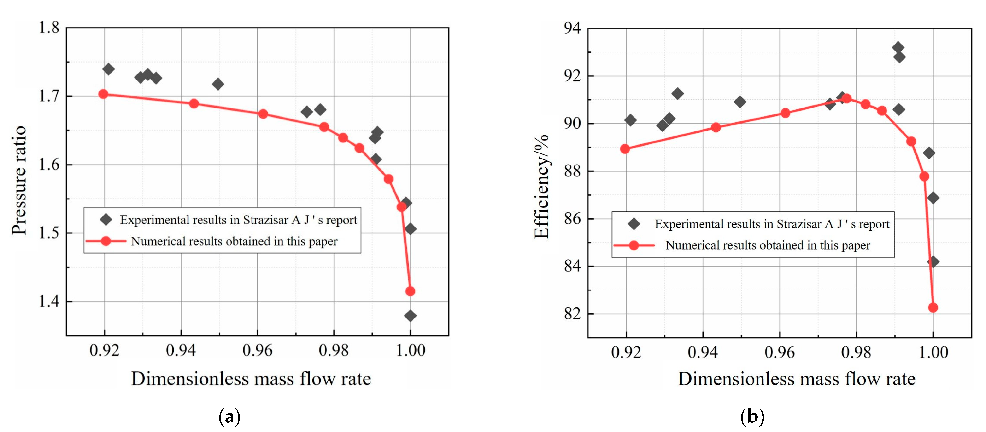
Figure 3 shows the pressure ratio and efficiency obtained via numerical calculation with the experimental data. The red curve is the fitting result of numerical calculations, and the black point is the test result. The pressure ratio and efficiency obtained using numerical calculations are in good agreement with the experimental data. In the whole flow rate range, the maximum error of the pressure ratio obtained via experiments and numerical simulations is less than 2.0%, and the maximum error of efficiency is less than 3.0%, which verifies the accuracy of the numerical method for the overall quantities analysis of compressor blades.
For an unsteady computation method, Zhu et al. [32] performed unsteady aerodynamic analysis on a 1.5-stage subsonic axial compressor through the same turbulence model and numerical method and compared it with experimental data [33,34]. The average error of efficiency between CFD and the experimental results is about 4%, while the maximum error of total pressure coefficients is about 0.8%. In addition, the main frequencies of the flow field obtained using CFD are consistent with experimental data. Therefore, the unsteady numerical method used in this study is appropriate and accurate.
2.3. Numerical Validation
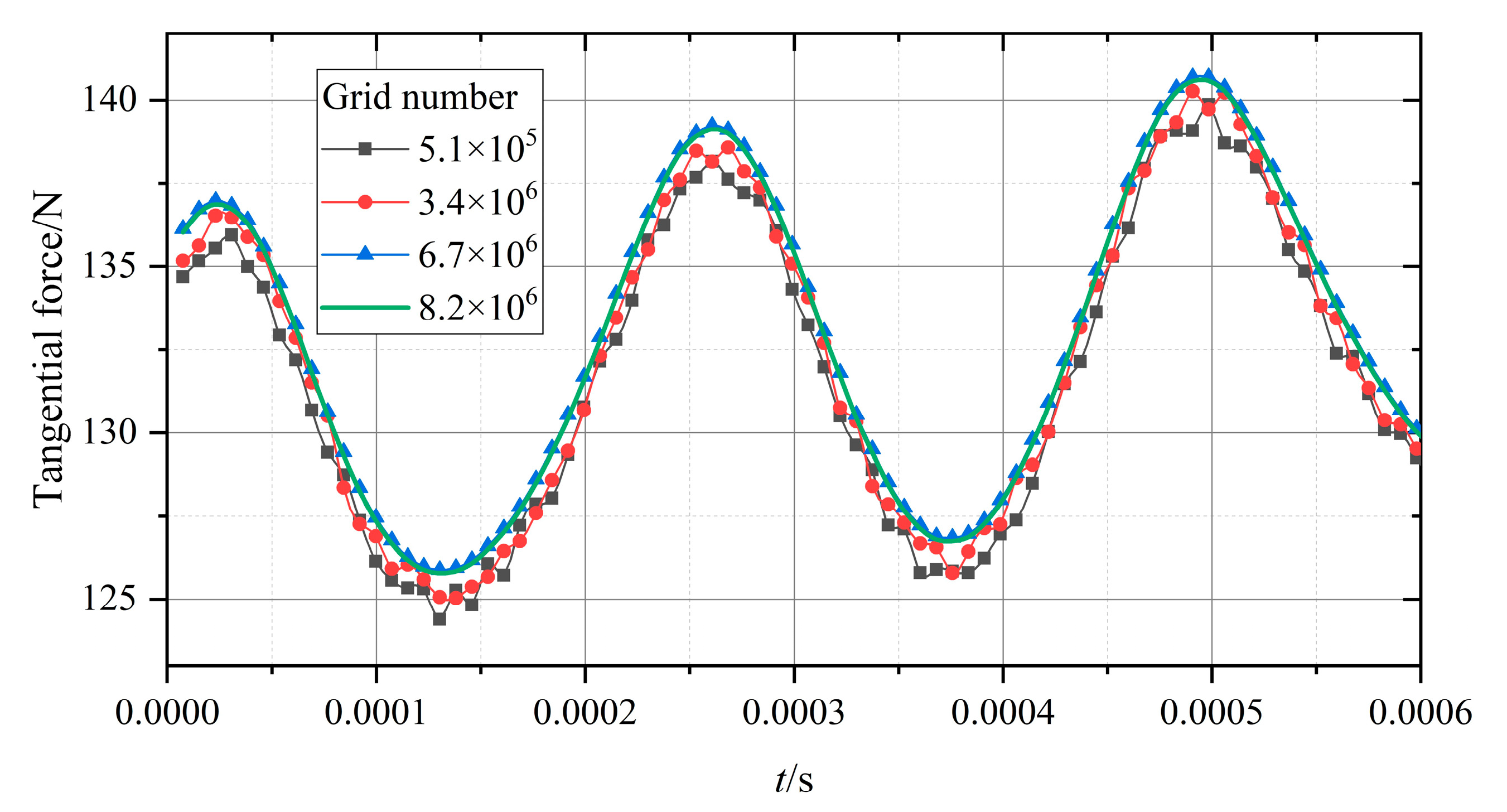
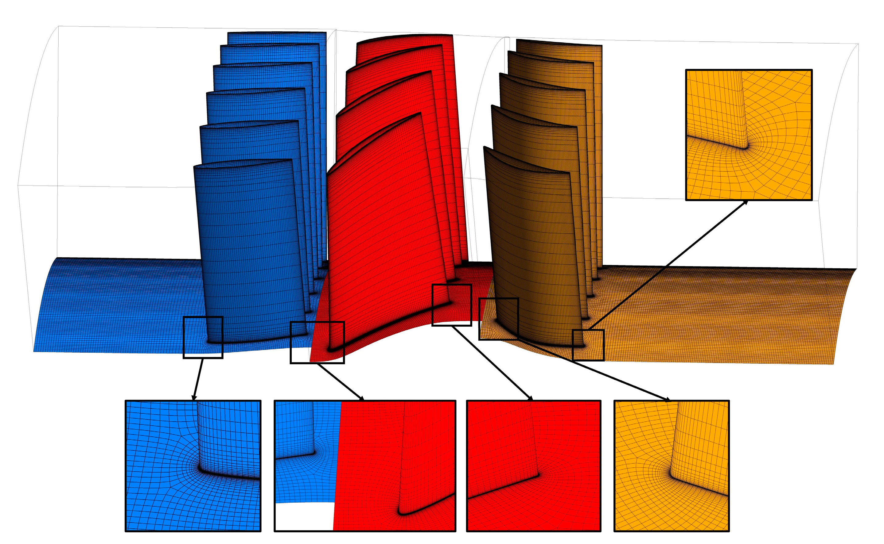
The whole fluid domain is divided into high-quality hexahedral grids. The O-type grid is applied around vanes and the H-type grid is mainly applied in the flow channels. The grids near the wall are densified to ensure the accuracy of the aerodynamic parameter calculations of the boundary layer. The value of y+ near the wall is less than 1. The grid is also densified at the trailing edge and leading edge to fully reflect the geometric characteristics. Taking the = 0 mm model as an example, Figure 4 shows the unsteady tangential force on the moving vane with different grid numbers under design condition. When the grid numbers increase from 6.7 million to 8.2 million, the maximum relative error of the tangential force is less than 0.1%. The number of grids is determined to be 6.7 million. Figure 5 shows the grids used in this study.
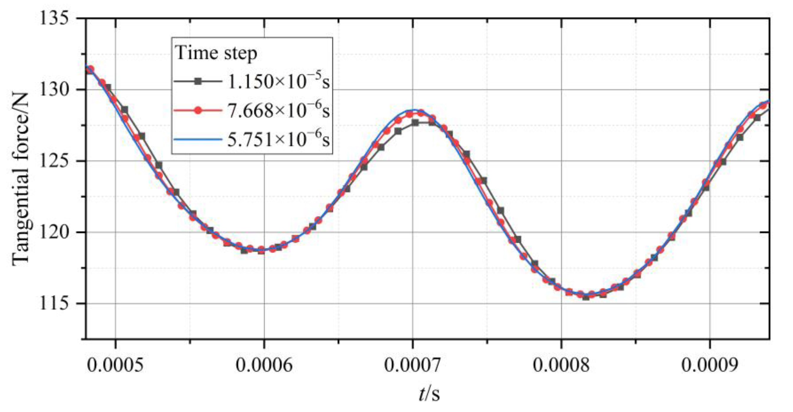
The time step used in the unsteady calculation is also verified. Taking the = 0 mm model as an example, Figure 6 shows the unsteady tangential force on the moving vane with different time steps under the design condition. The maximum error of the model with time steps of 7.668 × 10⁻⁶ s and 5.751 × 10⁻⁶ s is less than 0.2%. Therefore, setting the time step to 7.668 × 10⁻⁶ s can not only accurately show the unsteady parameters, but also do not increase the unnecessary calculation.
3. Results and Discussion
3.1. Unsteady Aerodynamic Results under the Design Condition
Table 3 shows the pressure ratio and total efficiency of different guide vane bending coefficients under the design condition. It can be seen that the guide vane bending coefficient has little effect on the overall aerodynamic performance. The pressure ratio decreases with the increase of . The pressure ratio of the = 10 mm model decreases by 0.18% compared with the = 0 mm model. The total efficiency of the “S”-type bowed models is reduced. The total efficiency of the structure with the = −10 mm decreases the most, which is 0.57%.
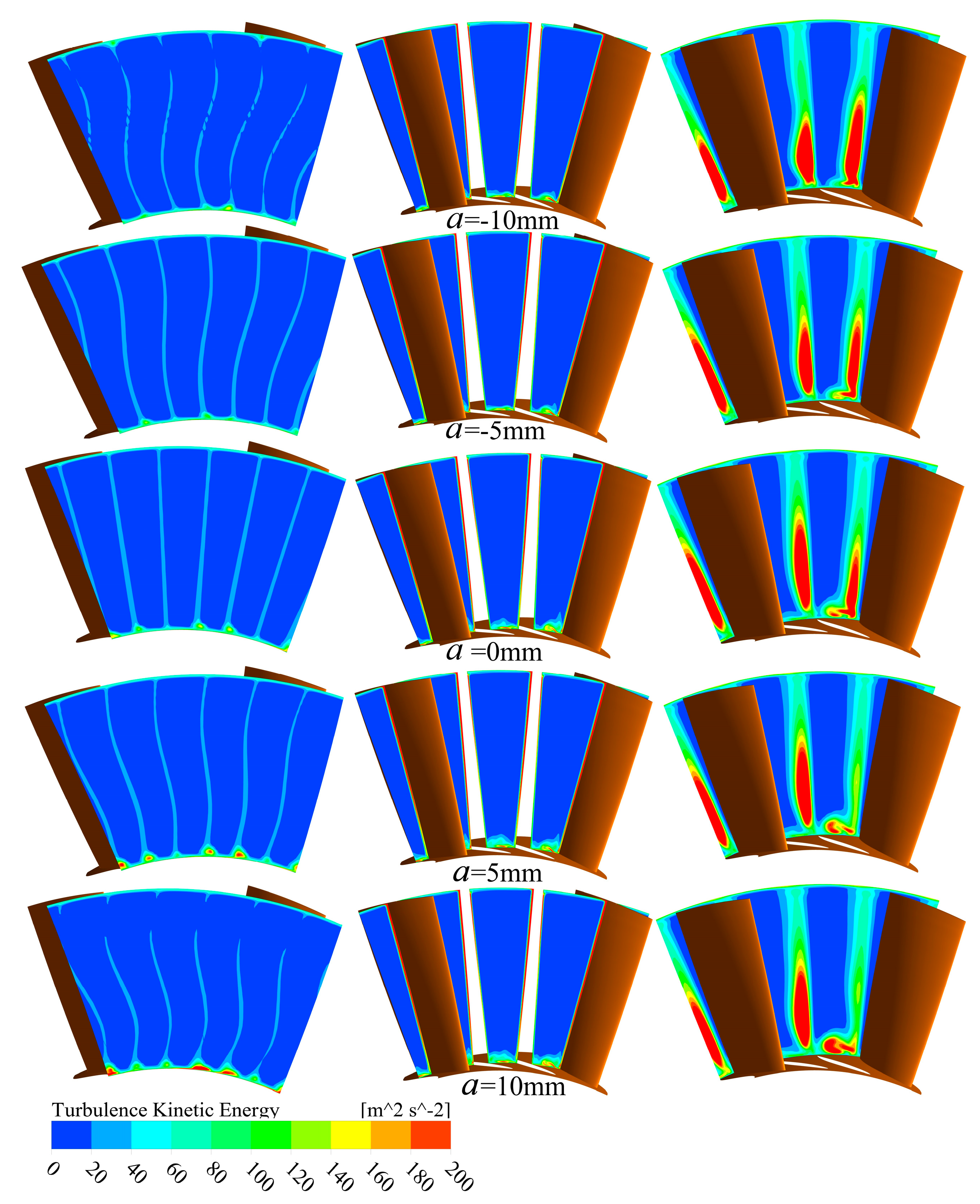
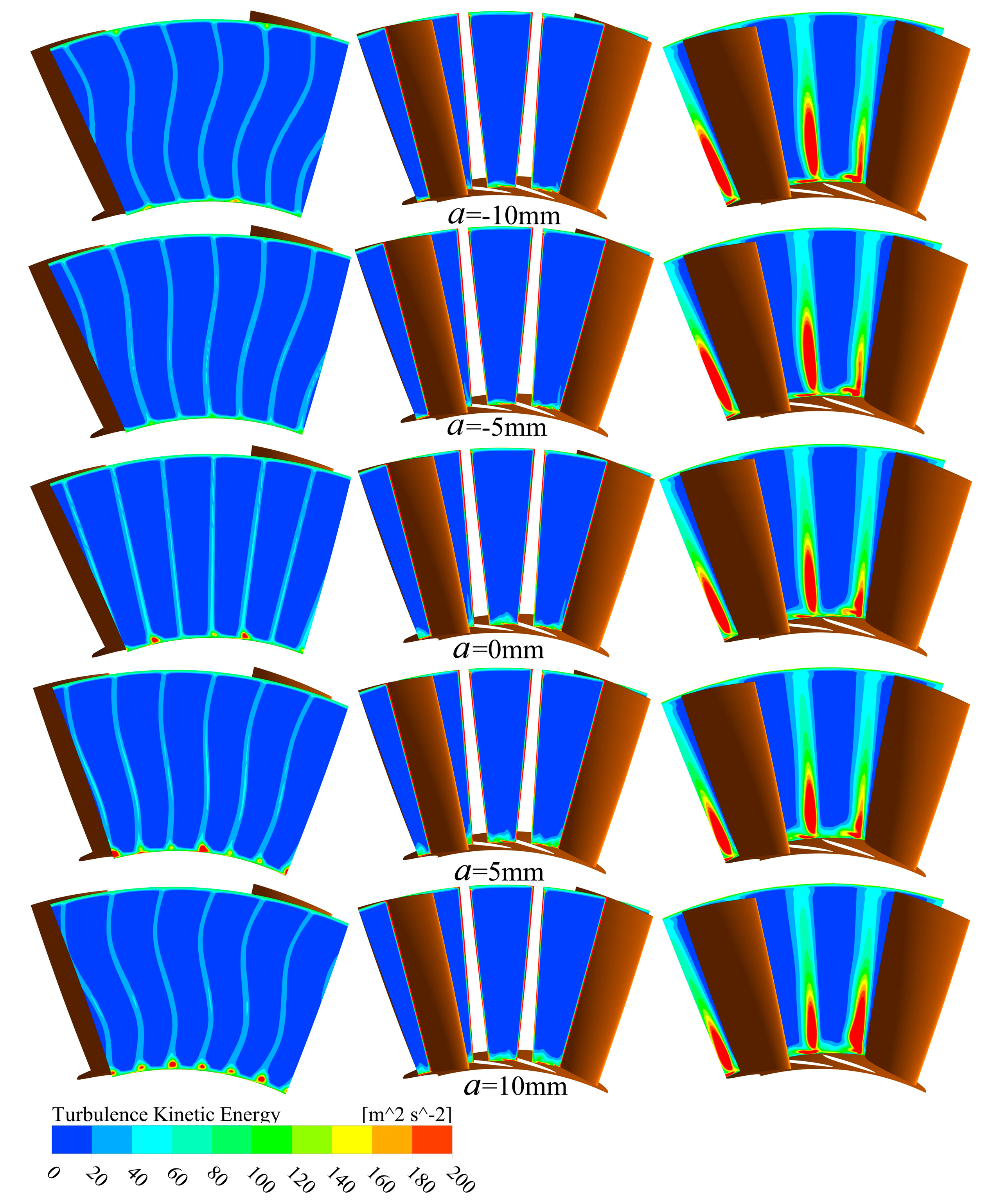
Figure 7 shows the turbulent kinetic energy distribution of models with different bending coefficients at different axial positions under the design condition at the time t = 0 T. The left figure is the front 2 mm position of the moving vane, which is the inflow of the moving vane. The middle figure is the middle position of the moving vane passage. The right figure is the back 2 mm position of the moving vane, which is downstream of the moving vane. It can be seen that, although the flow channels are geometrically symmetrical, the turbulent kinetic energy distribution of different flow channels is different, which is caused by the inherent unsteadiness of turbulence. At the inflow of the moving vane, the distribution of the high turbulent kinetic energy region is the same as the guide vane shape. This is because as the fluid flows downstream, the guide vane surface boundary layer changes to the turbulent boundary layer. The flow in the turbulent boundary layer is disordered. The turbulent boundary layers on both sides fall off and converge at the guide vane trailing edge, forming a wake area with higher turbulence intensity and more vortices. In addition, there are also regions with higher turbulent kinetic energy near the endwall, where the turbulent kinetic energy intensity near the hub is higher than that near the shroud. The area with higher turbulence kinetic energy regions near the shroud of the = −5 mm model is very small while that of the other models is large.
In the moving vane channel, the turbulent kinetic energy of the main flow area is low, and the areas with high turbulent kinetic energy are mainly concentrated on the moving vane surface and endwall, which is caused by the boundary layer. Among them, the turbulent kinetic energy near the hub is significantly higher. This is because the fluid domain of the moving vane is a rotating domain. Under the effect of centrifugal forces, the fluid in the moving vane channel tends to move in the radial direction, so the fluid near the hub is easier to perform flow separation. Among them, the turbulent kinetic energy of the = −5 mm model is the smallest near the hub. With the increase of , the turbulent kinetic energy near the hub shows an increasing trend. In addition, the intensity of turbulent kinetic energy near the suction surface of the moving vane is also significantly higher than that near the pressure surface. This is depended by the shape of the vane. The pressure surface is concave while the suction surface is convex. Fluid flow separation is more likely to occur when flowing through a convex surface.
Turbulent kinetic energy distribution downstream of the moving vane is also uneven in the circumferential direction according to the shape of the moving vane. The turbulent kinetic energy intensity is high in the wake area near the moving vane trailing edge, and low in the mainstream area near the middle of the moving vane channel. In the wake of the moving vane, the turbulent kinetic energy distribution along the blade height is also uneven. The turbulent kinetic energy intensity is higher at the position with a lower blade height. In the = 0 mm, = 5 mm, and = 10 mm models, the area near the hub with high turbulent kinetic energy is separated from the moving vane wake area, which has a great impact on the mainstream.
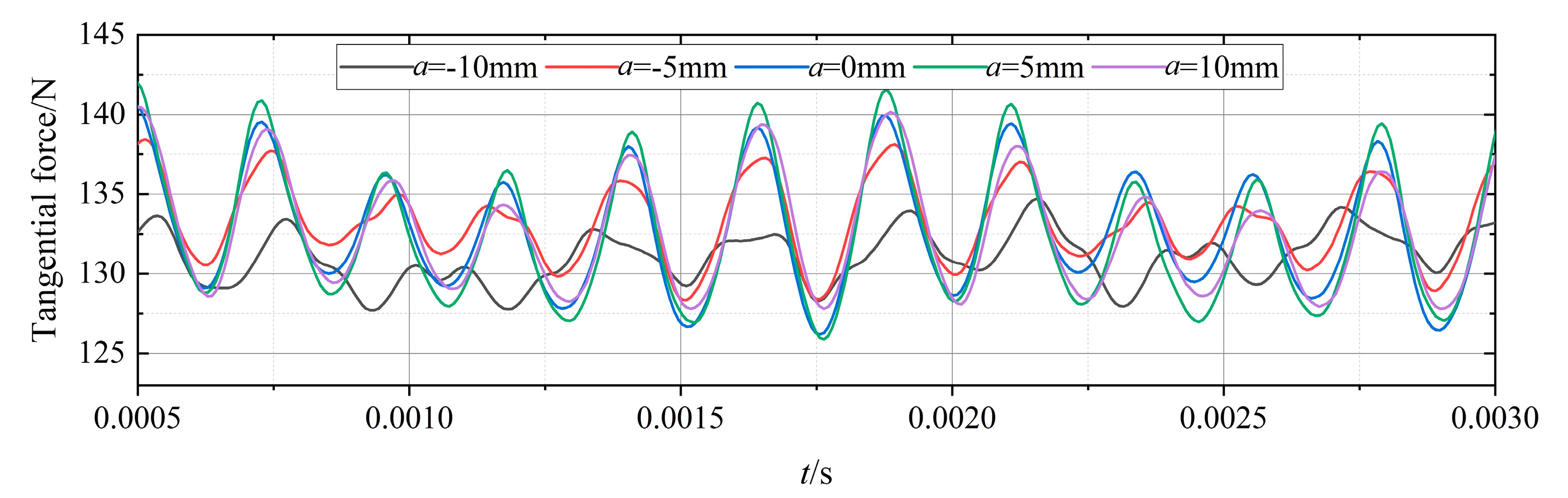
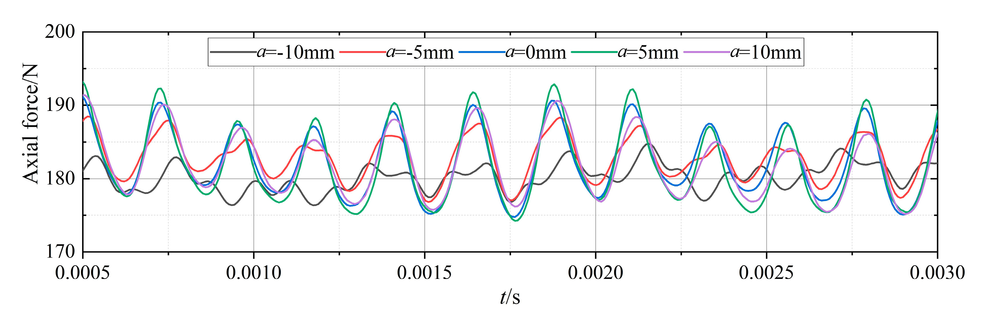
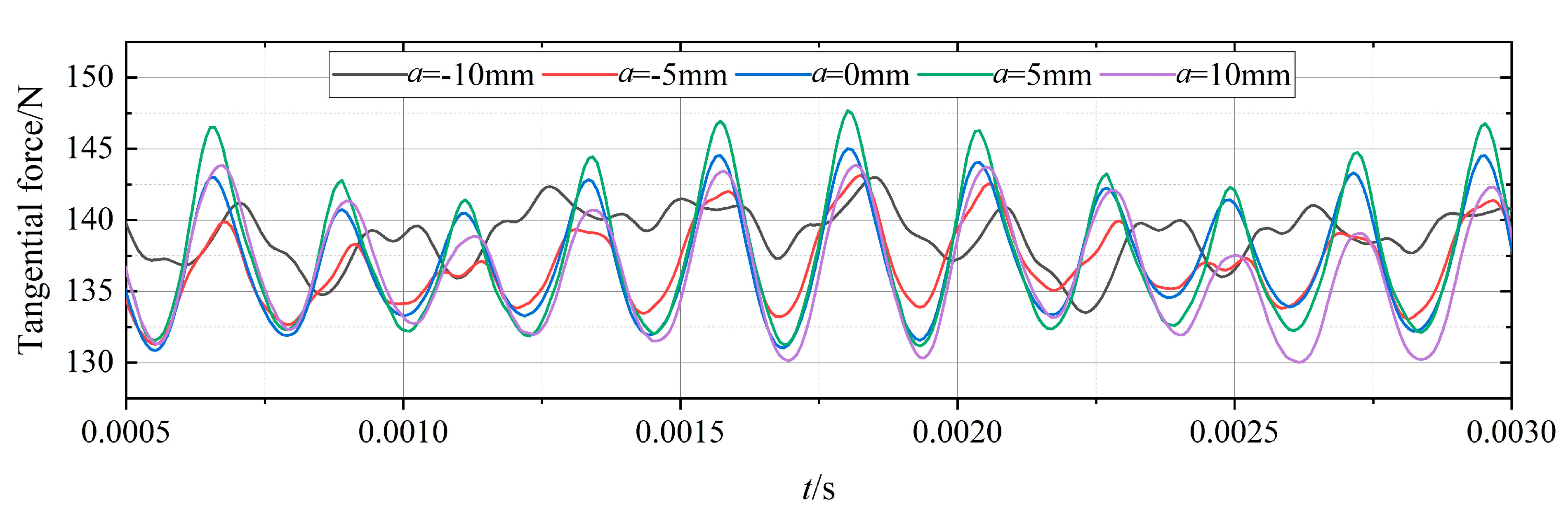
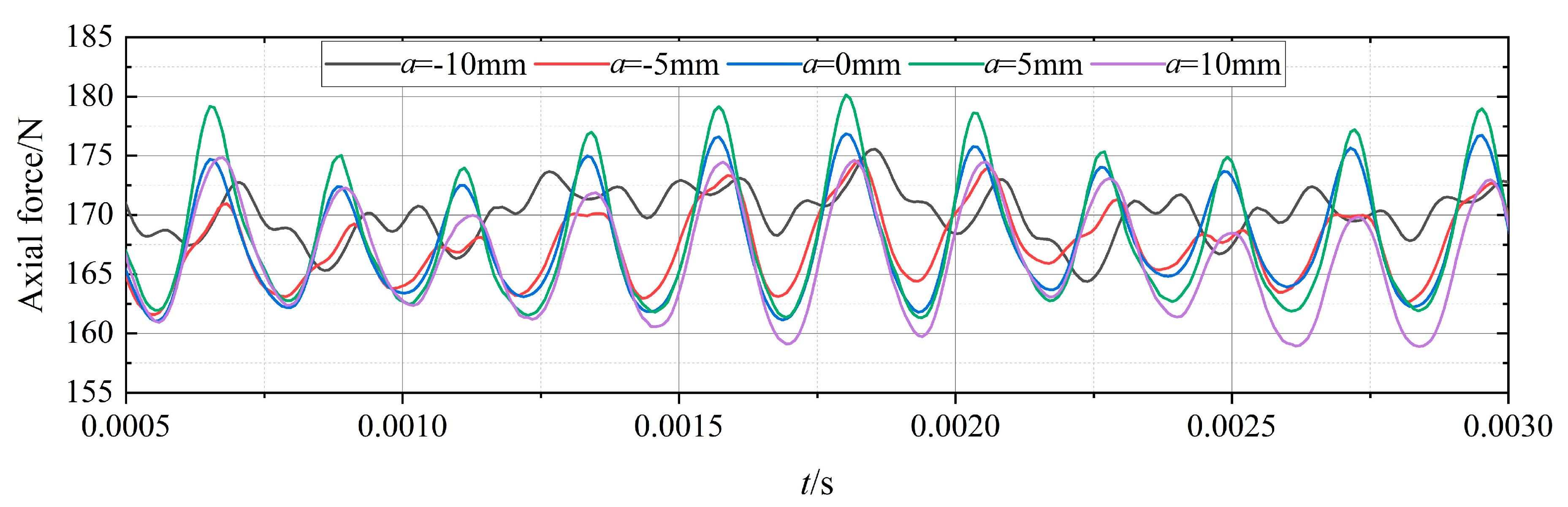
Figure 8 and Figure 9 show the tangential and axial exciting force–time domain distribution on moving vanes of different bending coefficient models under the design condition. It can be seen that the tangential and axial aerodynamic exciting forces show obvious periodicity. In the = −5 mm, = 0 mm, = 5 mm, and = 10 mm models, the time domain distribution of the exciting force is close to the form of sine functions. The time domain distribution of the aerodynamic exciting force of the = −10 mm model is very different from other models. Although the exciting force of the = −10 mm also shows a certain periodicity, its distribution is not in the form of a sine function, and the amplitude is significantly reduced compared with other models. The periodic aerodynamic exciting force will easily cause high-cycle fatigue fracture of the moving vane, reducing the service life of the blade. In addition, the phases of axial force and tangential force of different models are almost the same, which indicates that the tangential force and axial force reach the maximum and minimum values almost simultaneously. It means that the amplitude of the resultant force of the moving vane is larger, which is more unfavorable to the vibration safety of the blade.
Theoretically, the frequency of a high-frequency aerodynamic exciting force should be equal to the first-order blade-passing frequency. The number of guide vanes is 54 and the speed is 4830 rpm, so the time for a single moving vane to sweep through a guide vane channel is 2.3 × 10⁻⁴ s, and the first order blade-passing frequency is 4347 Hz.
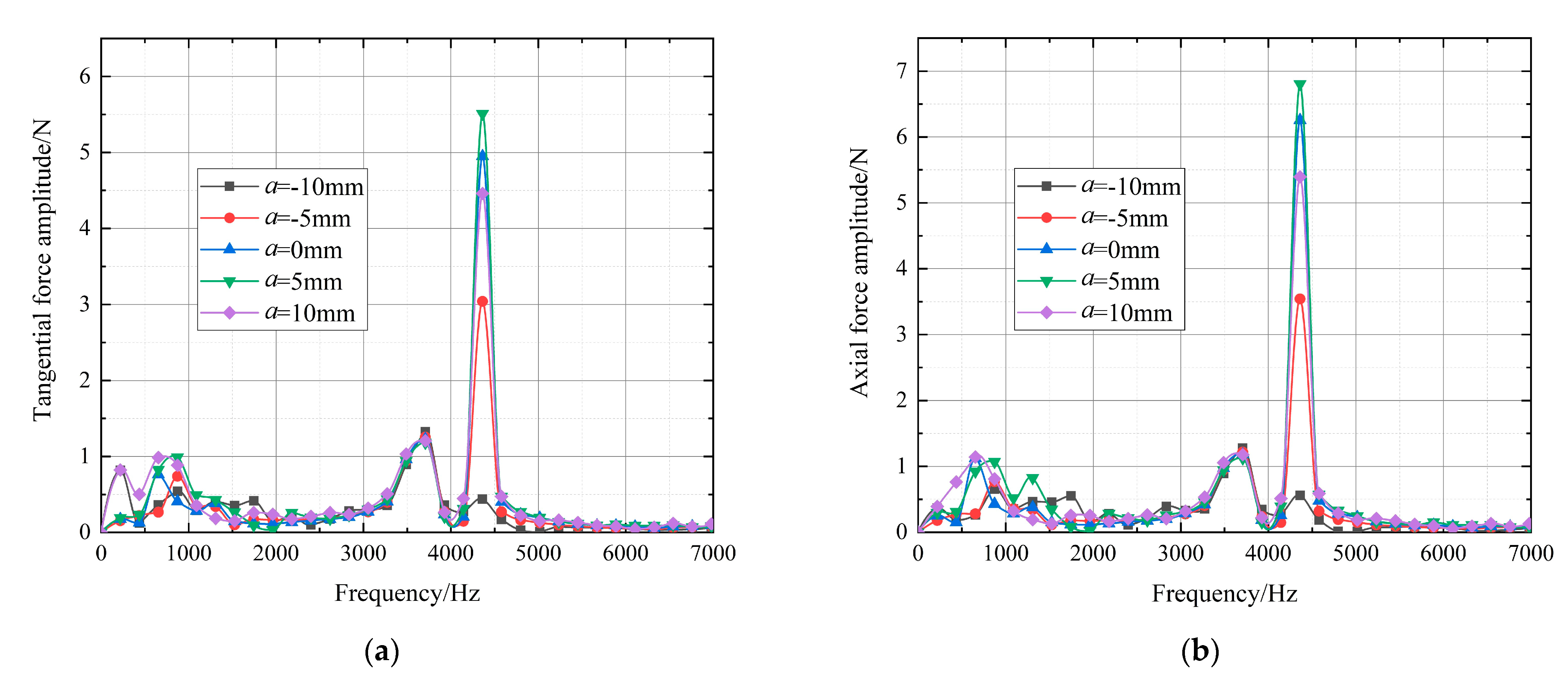
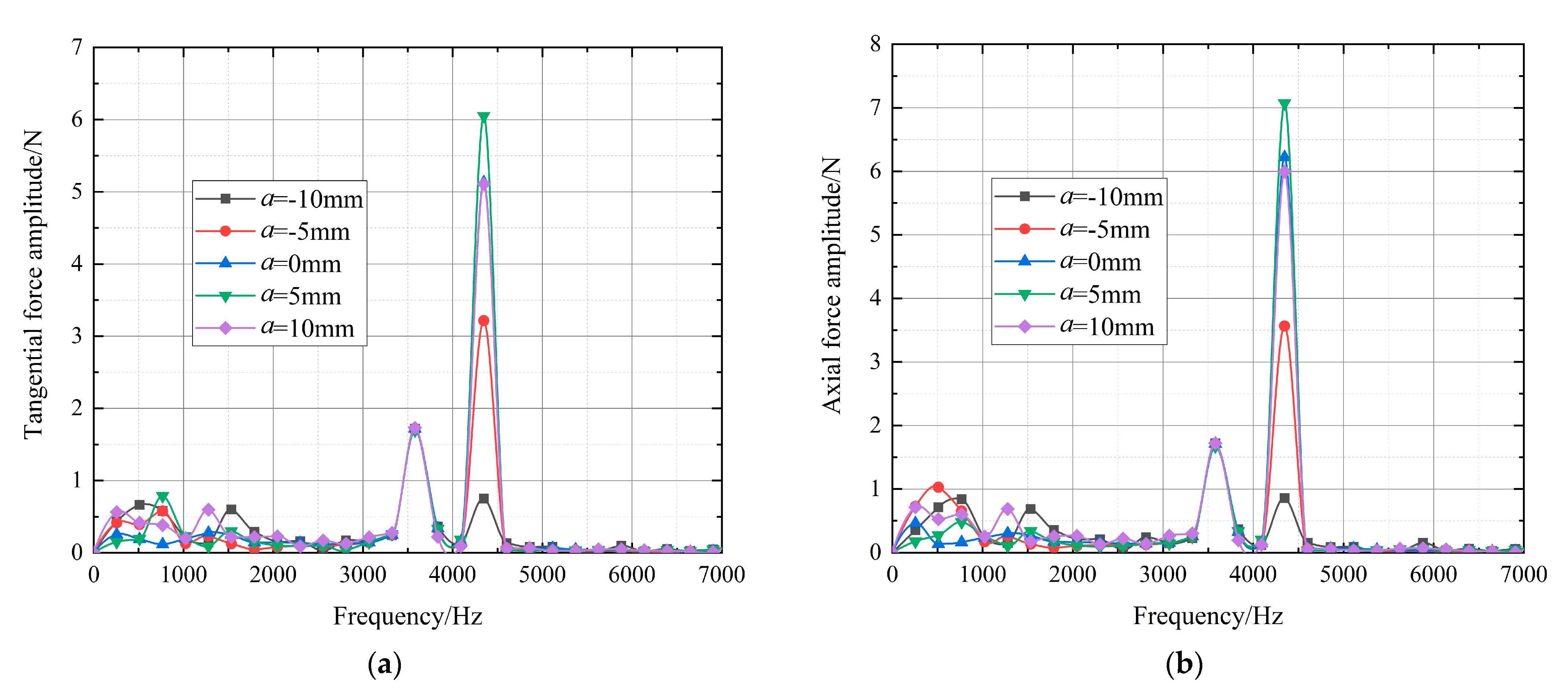
The time domain distribution of aerodynamic exciting forces is analyzed by using fast Fourier transform, and the frequency–domain distribution under design conditions shown in Figure 10 is obtained. It can be seen that, for models with different bending coefficients, there is a high local amplitude at the first-order blade-passing frequency, but the magnitude of the amplitude is very different. Table 4 shows the time mean value and the amplitude value at the first-order blade-passing frequency of aerodynamic exciting forces with different bending coefficients. Compared with the = 0 mm model, the aerodynamic exciting force amplitude of the = 5 mm model increases, in which the tangential exciting force amplitude increases by 14.89% and the axial exciting force amplitude increases by 14.35%. The aerodynamic exciting force amplitudes of the other models decreased, of which the = −10 mm model decreased the most, the tangential exciting force amplitude decreased by 90.82%, and the axial exciting force amplitude decreased by 90.39%.
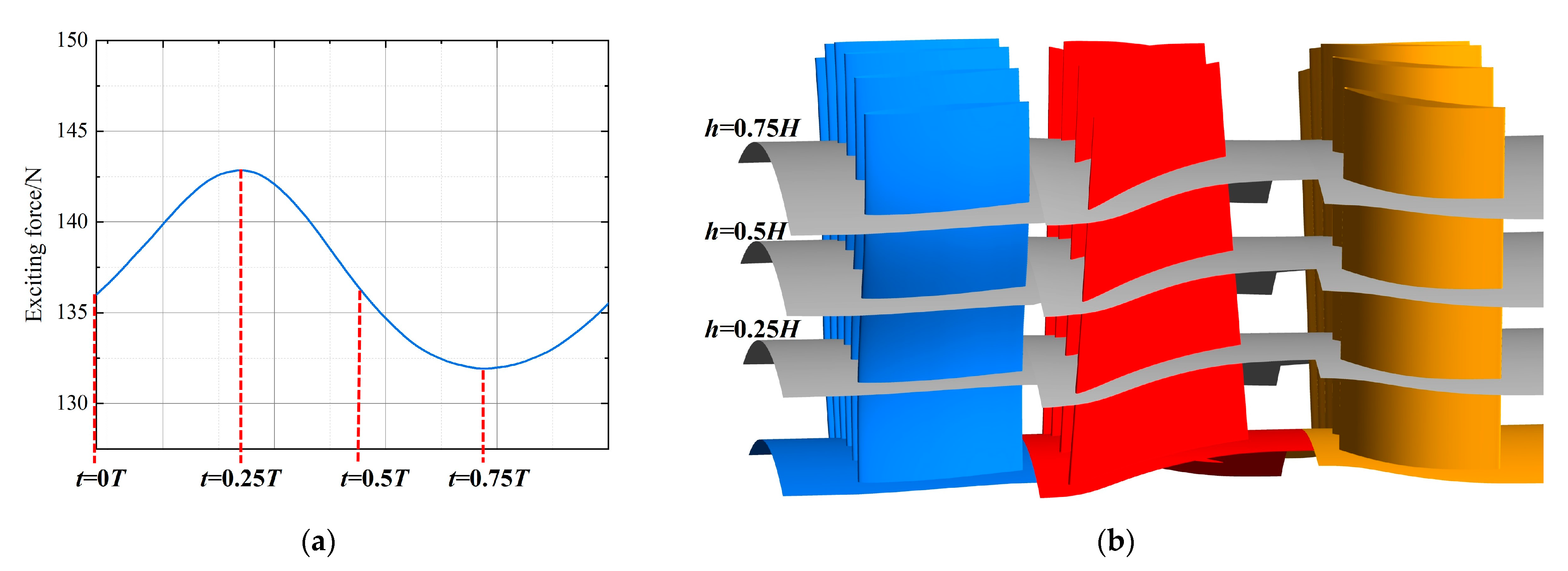
Since the time–domain distribution of the air flow exciting force has obvious periodicity, the time when a single moving vane sweeps through a guide vane channel is taken as a period, and four times are selected in each period to analyze the flow field characteristics. The time selection method is shown in Figure 11a, where 0.25 T is the time when the exciting force is the maximum and 0.75 T is the time when the aerodynamic exciting force is the minimum. In space, three section locations with different blade heights are selected for flow-field analysis. The selection method of blade–height section is shown in Figure 11b. For the “S”-type bowed guide vanes, 0.25 H and 0.75 H blade–height sections are the locations where the guide vane deviates most from the original model.
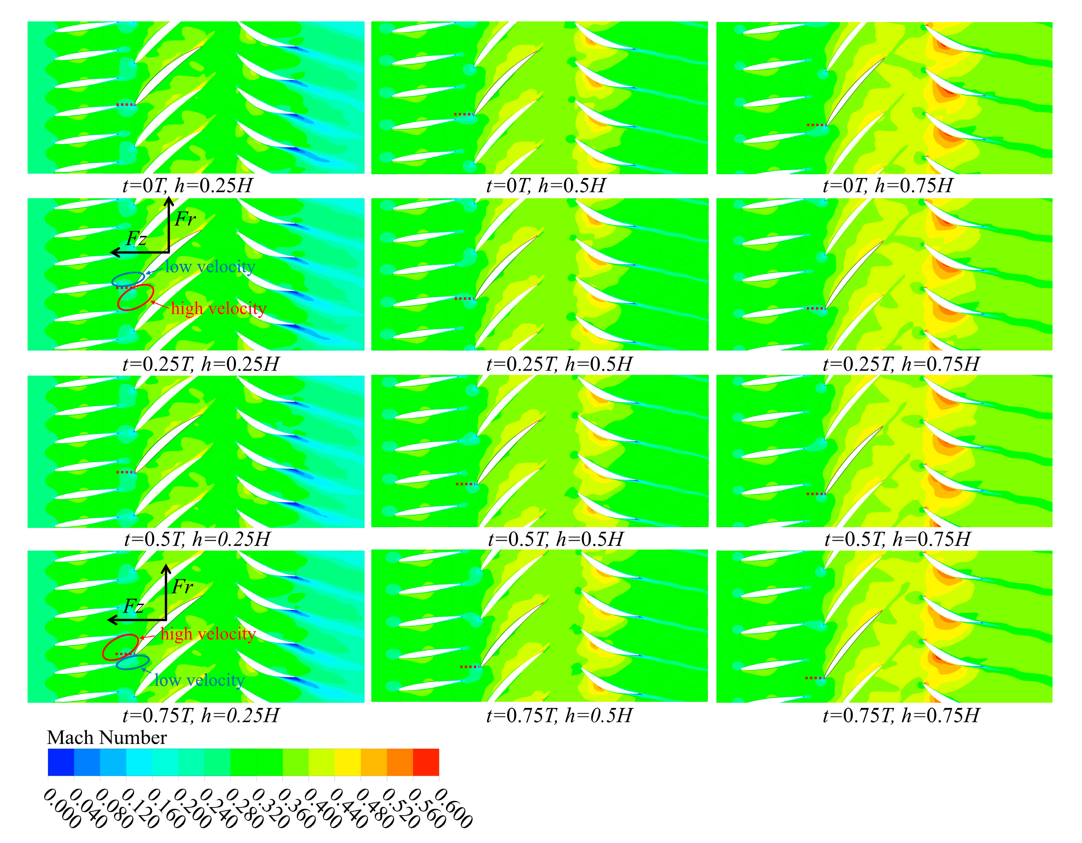
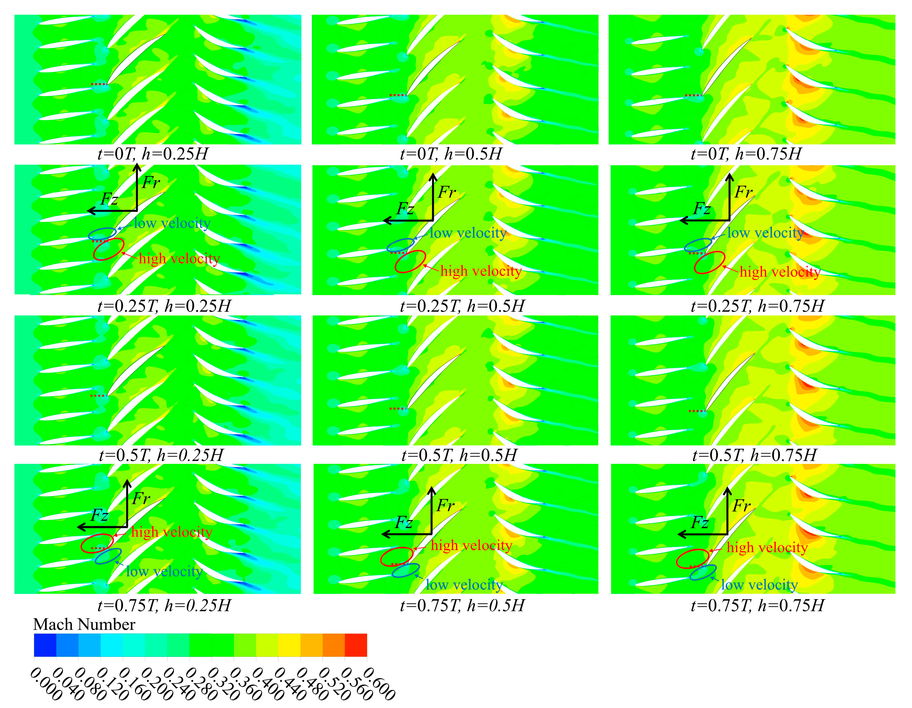
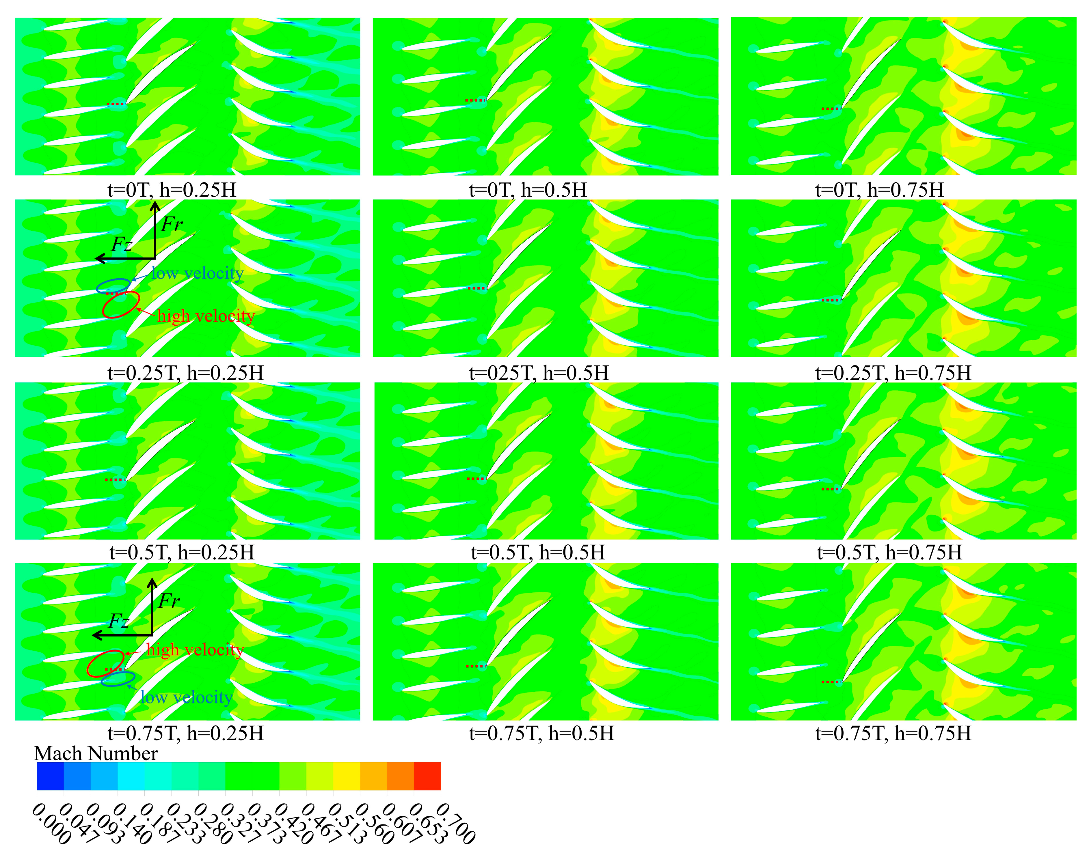
Figure 12 shows the Mach number distribution of different positions at different times of the model with a guide vane bending coefficient = 0 mm under the design condition. The moving vane with a black outline is the moving vane monitored in the unsteady aerodynamic calculation. The fluid forms a boundary layer on the guide vane surface. When the fluid flows out of the guide vane passage, the boundary layers on both sides fall off and converge at the trailing edge, forming a vortex zone with low velocity behind. The velocity of the mainstream near the middle of the guide vane channel is high, which results in uneven velocity distribution at the guide vanes outlet. The moving vanes will be alternately impacted by the high-speed fluid in the mainstream area and the low-speed fluid in the vortex area, so they will be subject to the periodic unsteady aerodynamic exciting force.
At the position of h = 0.25 H, the overall Mach number changes little from the inlet to the outlet of the guide vane. In the moving vane passage, the Mach number increases significantly. The Mach number near the pressure surface is relatively low while the Mach number near the suction surface is high. The maximum Mach number at the blade height of h = 0.25 H appears near the suction surface trailing edge. After the fluid flows through the stator vane passage, the Mach number gradually decreases along the flow direction, and a vortex zone with a lower flow velocity is formed behind the stator vanes trailing edge. The Mach number at the stator outlet is also relatively low, even lower than that at the guide vane inlet.
At the h = 0.5 H position, the flow field distribution in the guide vane and moving vane passage is similar to that at the position of h = 0.25 H, but the maximum Mach number appears at the stator vanes suction surface. The Mach number at the stator outlet is lower than that in the moving vane passage, but slightly higher than that at the guide vane inlet. At the h = 0.75 H position, the Mach number in the stator passage is further increased, a large area of the high Mach number appears on the pressure stator surface side, and the Mach number at the stator outlet is also significantly increased compared with that at the inlet of the guide vane. In summary, the Mach number tends to increase with the increase of the blade height. The increase at the downstream position is more obvious.
The red dotted line marks the relative position of the moving vane leading edge and the guide vane. For the = 0 mm model, although the guide vane is straight, the moving vane is designed to be twisted, so the relative position at different blade heights is slightly different. At t = 0.25 T, the moving vane leading edge is roughly at the position just passing the guide vane trailing edge, although relative positions of different blade heights are slightly different. We analyze the influence of the guide vane wake on the exciting force of the moving vane at this time. If there is no guide vane in this compressor stage, the moving vane incoming flow is uniform along the tangential direction. The flow force acting on the moving vane should be constant. The direction of the force is indicated by the black arrows in the figure. When the guide vane exists, the moving vane incoming flow is uneven. At the time t = 0.25 T, the low-speed fluid from the guide vane wake impacts the suction surface of the moving vane as shown in the blue circle, while the high-speed fluid from the main flow area of the guide vane impacts the pressure surface of the moving vane as shown in the red circle. Since the higher the speed, the higher the momentum, so the fluid force on both sides of the moving vane is different, and the fluid force on the pressure surface is higher than the suction surface. Since the direction of force caused by the uneven incoming flow is consistent with the direction of the aerodynamic force originally received by the moving vane, the aerodynamic force received by the moving vane reaches the maximum value at t = 0.25 T.
At the time t = 0.5 T, the moving vane leading edge rotates to the middle position of the guide vane channel, and the tangential force and axial force decrease. At time t = 0.75 T, with the rotation of the moving vane, the moving vane leading edge is close to the wake area of the next guide vane. The low-speed fluid in the guide vane wake area impacts the pressure surface of the moving vane, and the high-speed fluid in the main flow area of the guide vane impacts the suction surface. The fluid force on the suction surface is higher than that on the pressure surface. Since the direction of the force caused by the uneven incoming flow is opposite to the direction of the aerodynamic force originally received by the moving vane, the aerodynamic force received by the moving vane reaches the minimum value at t = 0.75 T.
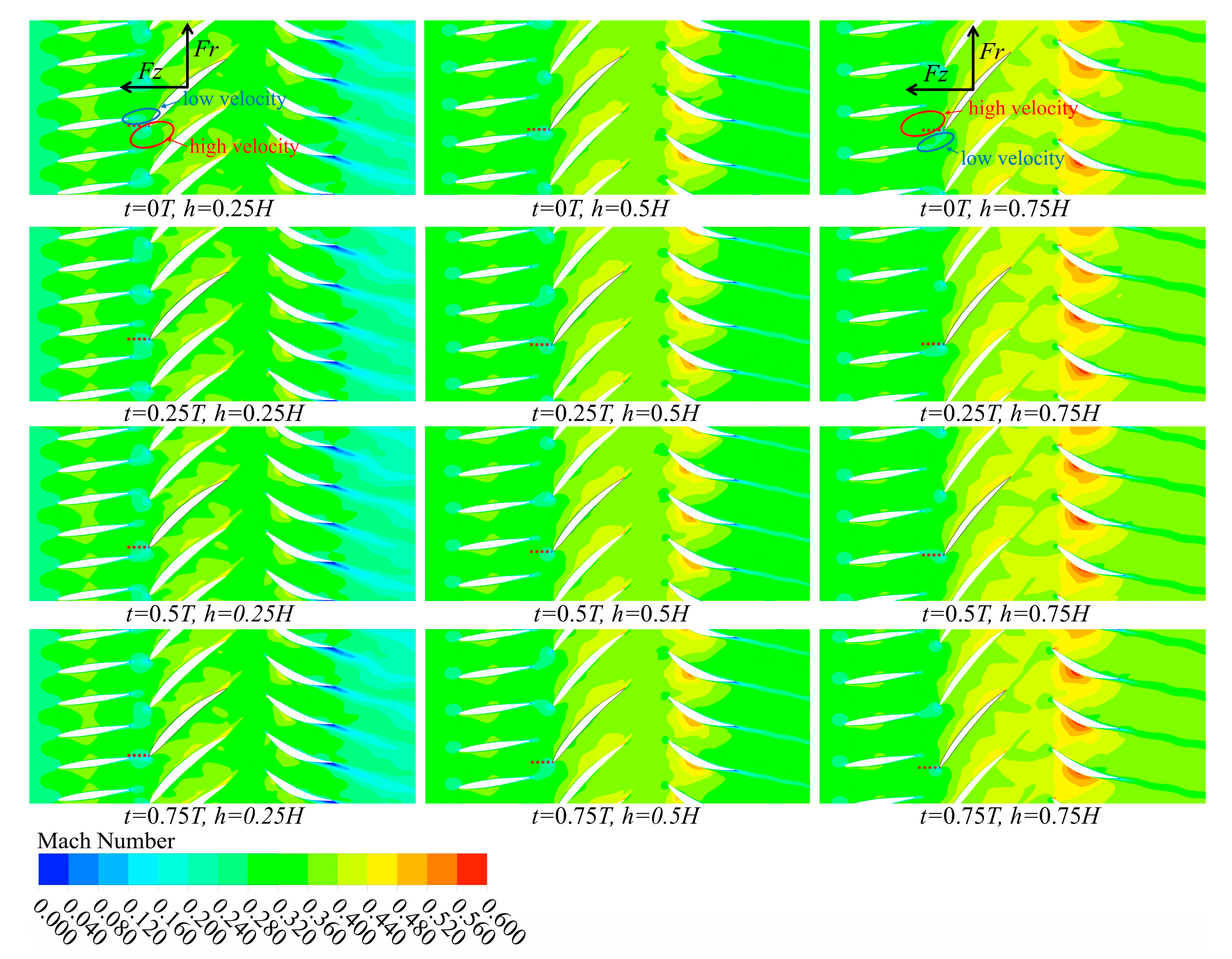
Since the aerodynamic exciting force amplitude of the = 5 mm model is the largest, the unsteady flow field distribution of the = 5 mm model is analyzed in detail. Figure 13 shows the Mach number distribution of different positions at different times of the model with a guide vane bending coefficient = 5 mm under the design condition. The overall distribution of the Mach number is basically consistent with that of the = 0 mm model. The Mach number tends to increase with the increase in blade height. The increase at the downstream position is more obvious. This shows that the = 5 mm model will not have too much deviation from the = 0 mm model in overall aerodynamic parameters.
The red dotted line marks the relative position of the moving vane leading edge and the guide vane. It can be seen that, at different blade heights, the relative position of the moving vane leading edge and the guide vane is almost the same. This results in that, at the same time, the influence of uneven flow field on the moving vane is almost the same at different blade heights.
At t = 0.25 T, the moving vane leading edge is roughly at the position just passing the guide vane trailing edge. The low-speed fluid from the guide vane wake impacts the suction surface of the moving vane as shown in the blue circle, while the high-speed fluid from the main flow area of the guide vane impacts the pressure surface of the moving vane as shown in the red circle. The fluid force on the pressure surface is higher than that on the suction surface. The direction of the force caused by the uneven incoming flow is consistent with the direction of the aerodynamic force originally received by the moving vane. Moreover, at different blade heights, the effect of increasing aerodynamic force is almost the same, which further increases the aerodynamic force.
At t = 0.75 T, the moving vane leading edge is roughly close to the trailing edge of the other guide vane. A low-speed fluid from the guide vane wake impacts the pressure surface of the moving vane as shown in the blue circle, while the high-speed fluid from the main flow area of the guide vane impacts the suction surface of the moving vane as shown in the red circle. The fluid force on the suction surface is higher than the pressure surface. The direction of the force caused by the uneven incoming flow is opposite to the direction of the aerodynamic force originally received by the moving vane. Furthermore, at different blade heights, the effect of reducing the aerodynamic force is almost the same, which further reduces the aerodynamic force at this time. Therefore, the = 5 mm model will increase the aerodynamic exciting force amplitude on the moving vane.
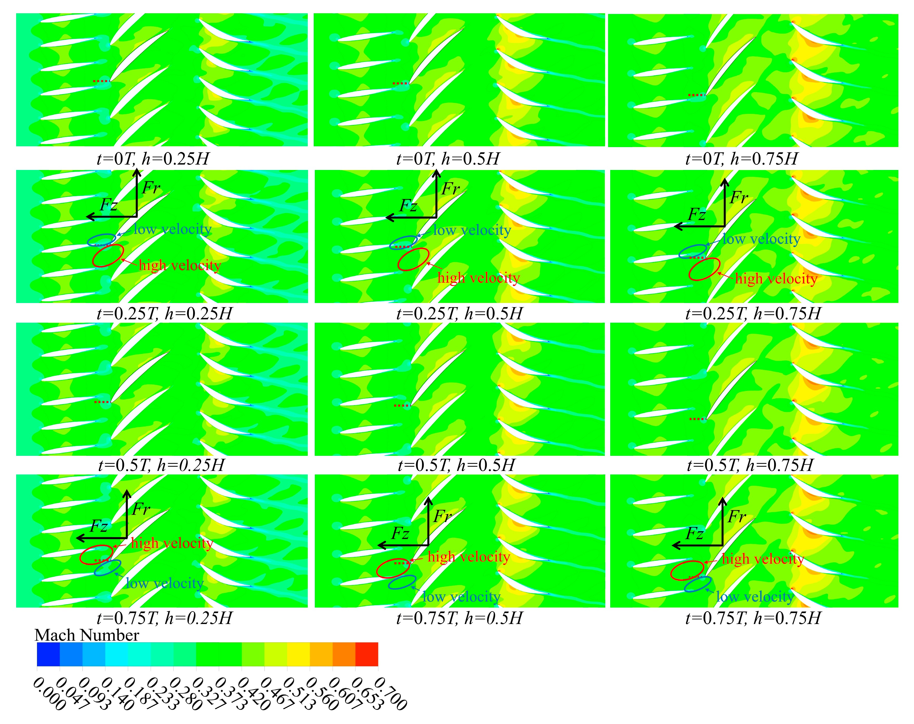
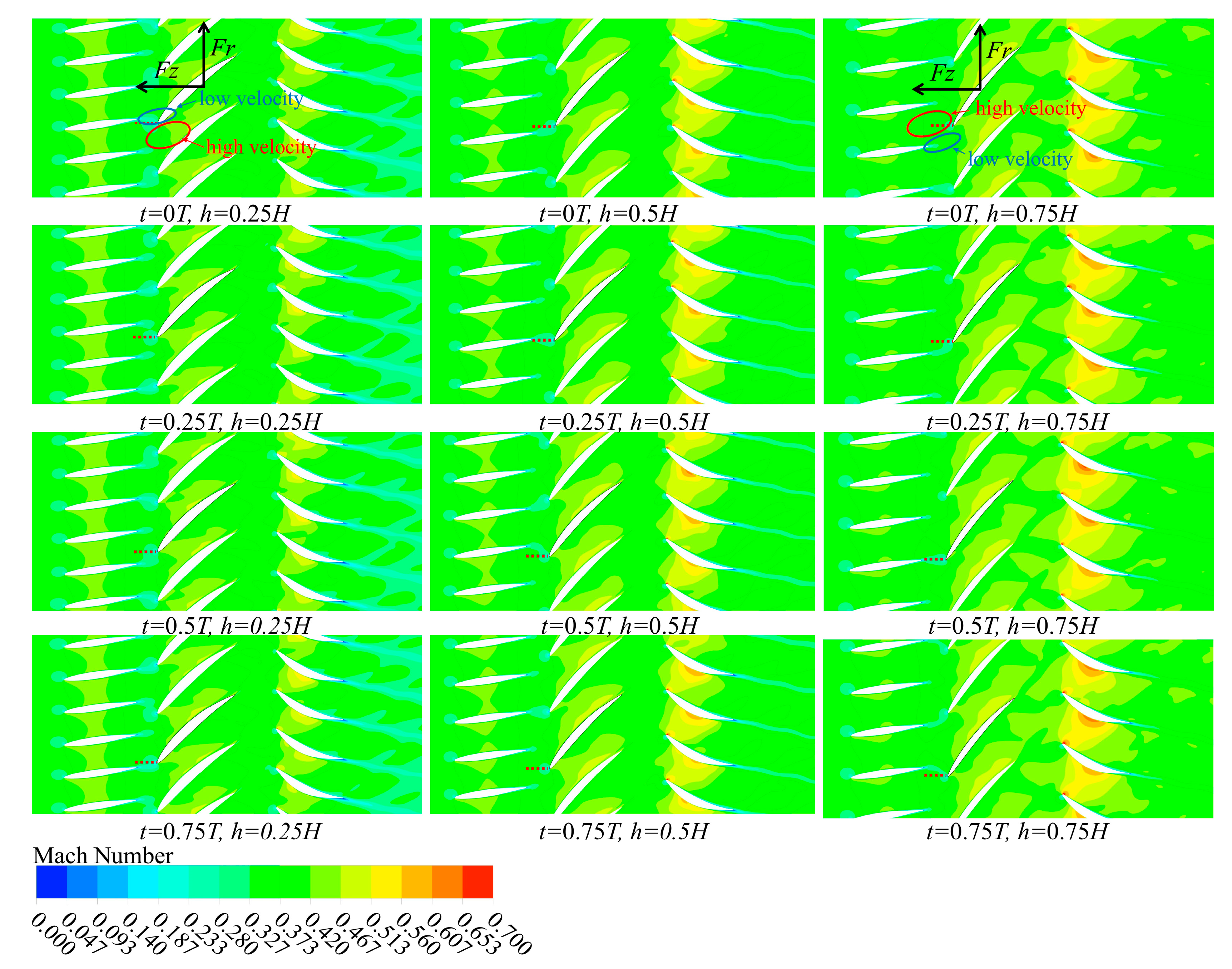
Since the aerodynamic exciting force amplitude of the = −10 mm model is minimal, the unsteady flow field distribution of the = −10 mm model is analyzed in detail. Figure 14 shows the Mach number distribution of different positions at different times of the model with a guide vane bending coefficient = −10 mm under design conditions. The overall distribution of the Mach number is basically consistent with that of the = 0 mm model. This shows that the = −10 mm model will also not have too much deviation from the = 0 mm model in overall aerodynamic parameters.
The red dotted line marks the relative position of the moving vane leading edge and the guide vane. It can be seen that, at different blade heights, the relative position difference between the moving vane leading edge and the guide vane is very large. Taking the time t = 0 T as an example, at h = 0.25 H, the moving vane leading edge is at the position just passing the trailing edge of the guide vane. A low-speed fluid from the guide vane wake impacts the suction surface of the moving vane, as shown in the blue circle, while the high-speed fluid from the main flow area of the guide vane impacts the pressure surface of the moving vane, as shown in the red circle. The fluid force on the pressure surface is higher than that on the suction surface. The direction of the force caused by uneven incoming flow is consistent with the direction of the aerodynamic force originally received by the moving vane. This increases the aerodynamic force on the moving vane.
At t = 0.75 T, the moving vane leading edge is roughly close to the trailing edge of the other guide vane. A low-speed fluid from the guide vane wake impacts the pressure surface of the moving vane, as shown in the blue circle, while the high-speed fluid from the main flow area of the guide vane impacts the suction surface of the moving vane, as shown in the red circle. The fluid force on the suction surface is higher than that on the pressure surface. The direction of the force caused by the uneven incoming flow is opposite to the direction of the aerodynamic force originally received by the moving vane. This will reduce the aerodynamic force on the moving vane. This means that, at different blade heights, the uneven flow field at the guide vane outlet may have the opposite effect on the force of the moving vane. Therefore, the amplitude of the exciting force on the moving vane of the = −10 mm model is very small, and the time–domain distribution curve of the exciting force is not like other models showing regular sine-like curves.
3.2. Unsteady Aerodynamic Results under Near-Blockage Conditions
Table 5 shows the pressure ratio and total pressure of different guide vane bending coefficients under near-blockage conditions. The effect of the guide vane bending coefficient on the overall aerodynamic performance is consistent with that of the design condition under the condition of near-blockage. The pressure ratio decreases with the increase in bending coefficients. When the bending coefficient = 10 mm, the pressure ratio decreases by 0.22% compared with the prototype. The total efficiency of the “S”-type bowed models is reduced. The total efficiency of the structure with = −10 mm decreases the most, which is 0.87%. In addition, the pressure ratio and total efficiency under the near-blockage condition are generally lower than that in the design condition.
Figure 15 shows the turbulent kinetic energy distribution of models with different bending coefficients at different axial positions of the moving vane under near-blockage conditions at the time t = 0 T. The left figure is the front 2 mm position of the moving vane, which is the inflow of the moving vane. The middle figure is the middle position of the moving vane passage. The right figure is the back 2 mm position of the moving vane, which is downstream of the moving vane.
The turbulent kinetic energy distribution of the near-blockage condition is similar to that of the design condition on the whole, but it is different locally. The difference is that the turbulent kinetic energy intensity in the guide vane wake region under the near-blockage condition is higher than that under design conditions. This is due to the greater flow of near-blockage conditions. When the boundary layer on the guide vane surface is transformed into a turbulent boundary layer, the turbulence intensity is higher, which leads to higher turbulent kinetic energy of the guide vane wake.
In addition, the turbulent kinetic energy intensity downstream of the moving vane under near-blockage conditions is obviously lower than that under the design conditions. This is because for the 1.5-stage axial compressor, the pressurization process is mainly completed in the rotor passage. Therefore, the flow in the moving vane channel is inverse the pressure gradient flow, which will cause more serious flow separation on the moving vane surface, making the turbulent kinetic energy of the moving vane wake larger. The pressure ratio of the near-clogging condition is smaller, so the flow separation caused by the inverse pressure gradient is lighter.
Figure 16 and Figure 17 show the tangential and axial exciting force–time domain distribution on the moving vane of different models under near-blockage conditions. In the = −5 mm, = 0 mm, = 5 mm, and = 10 mm models, the time–domain distribution is close to the form of the sine function. The time–domain distribution of the aerodynamic exciting force of the = −10 mm model is very different from other models.
The time–domain distribution of the air flow exciting force under near-blockage conditions is analyzed using a fast Fourier transform, and the spectrum distribution is obtained as shown in Figure 18. The amplitude of the = −10 mm model is much lower than that of other models.
Table 6 shows the time mean value and the amplitude value at the first-order blade-passing frequency of the aerodynamic exciting force with different bending coefficients. Compared with the design condition, the mean value of the tangential force increased slightly, the mean value of the axial force decreased, and the amplitude of the exciting force under each model increased compared with the design condition. It can be seen that, compared with the = 0 mm model, the aerodynamic exciting force amplitude of the = 5 mm model increases, in which the tangential exciting force amplitude increases by 19.09% and the amplitude of the axial exciting force increases by 17.19%. The aerodynamic exciting force amplitudes of the other models decreased, of which the = −10 mm model decreased the most, the tangential exciting force amplitude decreased by 85.84%, and the axial exciting force amplitude decreased by 86.58%.
Figure 19 shows the Mach number distribution for the = 0 mm model under the near-blockage conditions. The overall Mach number of the near blocking condition is higher than that of the design condition. At the position of h = 0.25 H, the Mach number of the stator outlet is almost the same as the inlet Mach number of the guide vane in the near-blockage condition, which is different from the design condition.
In addition, at the position of h = 0.75 H, the Mach number in the stator passage is not much higher than that in the guide vane and moving vane passage. The Mach number difference of different blade heights is reduced in the near-blockage condition compared to the design condition. At the time t = 0.25 T, the exciting force on the moving vane is the largest, and the leading edge of the moving vane is at the position just passing the guide vane trailing edge. At the time t = 0.75 T, the exciting force on the moving vane is the smallest, and the leading edge of the moving vane is at the position near the trailing edge of the next guide vane. The relative position of the moving vane and guide vane is consistent with that under the design condition.
Under the near-blockage condition, the aerodynamic exciting force amplitude of the = 5 mm model is the highest and the aerodynamic exciting force amplitude of the = −10 mm model is the lowest. Figure 20 and Figure 21 show the Mach number distributions of = 5 mm and = −10 mm under near-blocking conditions. The Mach number distribution of different models is not much different. It shows that the “S”-type bowed guide vane will not have a great impact on the overall aerodynamic performance under near-blockage conditions. The reason for the increase and decrease of the aerodynamic exciting force amplitude is the same as that of the design condition, which is determined by the relative position of the moving vane and the guide vane of different blade heights. The reason for the change of the aerodynamic exciting force amplitude is the same as that of the design condition, which is determined by the relative position of the moving vane and the guide vane at different blade heights.
4. Conclusions
In this study, an “S”-type bowed guide vane was designed, and a 1.5-stage axial compressor model was established. For five guide vane models with different bending coefficients, an unsteady numerical simulation was carried out under the design condition and the near-blockage condition. The influence of the “S”-type bowed guide vane on the overall aerodynamic performance, unsteady flow field distribution, and air flow exciting force is analyzed. The main conclusions are as follows:
- (1)
- The pressure ratio decreases with the increase in the guide vane bending coefficient. Compared with the original straight vane, the pressure ratio under the design condition and the near-blockage condition decreases by 0.18% and 0.22%, respectively, in the = 10 mm models. The total efficiency of the model with the “S”-type bowed guide vane is reduced. The total efficiency of the = −10 mm model decreases the most, which is 0.57% and 0.87% in the design condition and near-blockage condition, respectively.
- (2)
- The turbulence kinetic energy near the hub of the guide vane will increase with the increase in the absolute value of the bending coefficient. The turbulence kinetic energy of the guide vane wake under the near-blockage condition is higher than that under the design condition due to the higher velocity. However, in the moving vane passage and the wake of the moving vane, due to the low-pressure ratio under the near-blockage condition, the flow separation caused by the inverse pressure gradient is relatively small.
- (3)
- The = 5 mm model will increase the aerodynamic exciting force amplitude on the moving vane. The = −10 mm model can reduce the tangential and axial aerodynamic exciting force amplitudes under the first-order blade-passing frequency of the moving vane by 90.82% and 90.39% under the design condition, respectively. Under the near-blockage condition, the reduced values are 85.84% and 86.58%, respectively. This is because, for the = −10 mm model, at different blade heights, the relative position difference between the moving vane leading edge and the guide vane is very large. This means the uneven flow field at the guide vane outlet may have the opposite effect on the force of the moving vane at different blade heights.
This shows that the “S”-type bowed guide vanes can greatly reduce the aerodynamic exciting force amplitude under the premise of reducing aerodynamic efficiency, which provides an idea for compressor design under some conditions with extremely high requirements for vibration safety. Subsequently, we can consider the design of the moving vane near the end wall to improve the efficiency of the compressor with the “S”-type bowed guide vanes.
Author Contributions
Each author has contributed to different work in this study. Y.L. (Yupeng Liu) is mainly responsible for data curation, methodology and writing—original draft. The validation and visualization were completed by Y.L. (Yunzhu Li); G.L., Y.X. and D.Z. undertook the task of writing—review and editing. All authors have read and agreed to the published version of the manuscript.
Funding
This research was funded by the National Science and Technology Major Project grant number [J2019-IV-0022-0090].
Institutional Review Board Statement
Not applicable.
Informed Consent Statement
Not applicable.
Data Availability Statement
Data sharing is not applicable to this article.
Acknowledgments
All the authors in the paper express great gratitude for the financial support by the National Science and Technology Major Project (J2019-IV-0022-0090).
Conflicts of Interest
The authors declare that they have no known competing financial interest or personal relationships that could have appeared to influence the work reported in this paper.
References
- Matsunuma, T. Unsteady flow field of an axial-flow turbine rotor at a low Reynolds number. J. Turbomach. 2007, 129, 360–371. [Google Scholar] [CrossRef]
- Maroldt, N.; Amer, M.; Seume, J.R. Forced Response Due to Vane Stagger Angle Variation in an Axial Compressor. J. Turbomach. 2022, 144, 081011. [Google Scholar] [CrossRef]
- Gallus, H.E.; Lambertz, J.; Wallmann, T. Blade-Row Interaction in an Axial-Flow Subsonic Compressor Stage. J. Eng. Power 1980, 102, 169–177. [Google Scholar] [CrossRef]
- Gallus, H.E.; Grollius, H.; Lambertz, J. The Influence of Blade Number Ratio and Blade Row Spacing on Axial-Flow Compressor Stator Blade Dynamic Load and Stage Sound Pressure Level. J. Eng. Power 1982, 104, 633–641. [Google Scholar] [CrossRef]
- Gorrell, S.E.; Okiishi, T.H.; Copenhaver, W.W. Stator-Rotor Interactions in a Transonic Compressor—Part 1: Effect of Blade-Row Spacing on Performance. J. Turbomach. 2003, 125, 328–335. [Google Scholar] [CrossRef]
- Douglas, M.B.; Sanford, F. Axial Compressor Blade-to-Blade Unsteady Aerodynamic Variability. J. Propuls. Power 2015, 19, 242–249. [Google Scholar]
- Burkhardt, O.; Nitsche, W.; Goller, M.; Swoboda, M.; Guemmer, V. Rotor-stator interaction in a highly-loaded, single-stage, low-speed axial compressor: Unsteady measurements in the rotor relative frame. In Unsteady Aerodynamics, Aeroacoustics and Aeroelasticity of Turbomachines; Hall, K.C., Kielb, R.E., Thomas, J.P., Eds.; Springer: Dordrecht, The Netherlands; Berlin/Heidelberg, Germany, 2006; pp. 603–614. [Google Scholar]
- Smith, N.R.; Key, N.L. Unsteady vane boundary layer response to rotor–rotor interactions in a multistage compressor. J. Propuls. Power 2014, 30, 416–425. [Google Scholar] [CrossRef]
- Lefcort, M.D. An Investigation into Unsteady Blade Forces in Turbomachines. J. Eng. Power 1965, 87, 345–354. [Google Scholar] [CrossRef]
- Daigji, H.; Shirahara, H. A finite element solution of cascade flow in a large-distorted periodic flow. Bull. JSME 1978, 21, 824–831. [Google Scholar] [CrossRef]
- Mailach, R.; Müller, L.; Vogeler, K. Rotor-stator interactions in a four-stage low-speed axial compressor—Part II: Unsteady aerodynamic forces of rotor and stator blades. J. Turbomach. 2004, 126, 519–526. [Google Scholar] [CrossRef]
- Smith, N.R.; Key, N.L. Blade-row interaction effects on unsteady stator loading in an embedded compressor stage. J. Propuls. Power 2017, 33, 248–255. [Google Scholar] [CrossRef]
- Monk, D.J.; Key, N.L.; Fulayter, R.D. Reduction of aerodynamic forcing through introduction of stator asymmetry in axial compressors. J. Propuls. Power 2016, 32, 134–141. [Google Scholar] [CrossRef]
- Wenjie, W.; Peter, J.T. Acoustic Improvement of Stator-Rotor Interactionwith Nonuniform Trailing Edge Blowing. Appl. Sci. 2018, 8, 994–1004. [Google Scholar]
- Milidonis, K.; Semlitsch, B.; Hynes, T. Effect of Clocking on Compressor Noise Generation. AIAA J. 2018, 56, 4225–4231. [Google Scholar] [CrossRef]
- Weir, D.S.; Podboy, G.G. Flow Measurements and Multiple Pure Tone Noise from a Forward Swept Fan. In Proceedings of the 43rd AIAA Aerospace Sciences Meeting and Exhibit, Reno, NV, USA, 10–13 January 2005. [Google Scholar]
- Bamberger, K.; Carolus, T. Optimization of axial fans with highly swept blades with respect to losses and noise reduction. Noise Control. Eng. J. 2012, 60, 716–725. [Google Scholar] [CrossRef]
- Bohn, D.E.; Ren, J.; Tümmers, C.; Sell, M. Unsteady 3D-numerical investigation of the influence of the blading design on the stator-rotor interaction in a 2-stage turbine. In Proceedings of the ASME Turbo Expo 2005: Power for Land, Sea, and Air, Reno, NV, USA, 6–9 June 2005. [Google Scholar]
- Laborderie, J.D.; Blandeau, V.; Node-Langlois, T.; Moreau, S. Extension of a Fan Tonal Noise Cascade Model for Camber Effects. AIAA J. 2015, 53, 863–876. [Google Scholar] [CrossRef]
- Ling, J.; Du, X.; Wang, S.; Wang, Z. Relationship between optimum curved blade generate line and cascade parameters in subsonic axial compressor. In Proceedings of the ASME Turbo Expo 2014: Turbine Technical Conference and Exposition, Düsseldorf, Germany, 16–20 June 2014. [Google Scholar]
- Rajesh, E.; Roy, B. Numerical study of variable camber inlet guide vane on low speed axial compressor. In Proceedings of the ASME 2015 Gas Turbine India Conference, Hyderabad, India, 2–3 December 2015. [Google Scholar]
- Wadia, A.R.; Szucs, P.N.; Gundy-Burlet, K.L. Design and Testing of Swept and Leaned Outlet Guide Vanes to Reduce Stator–Strut–Splitter Aerodynamic Flow Interactions. J. Turbomach. 1999, 121, 416–427. [Google Scholar] [CrossRef]
- Keke, G.; Yonghui, X.; Di, Z. Effects of stator blade camber and surface viscosity on unsteady flow in axial turbine. Appl. Therm. Eng. 2017, 118, 748–764. [Google Scholar]
- Chen, X.; Chu, W.; Wang, G.; Yan, S.; Shen, Z.; Guo, Z. Effect of span range of variable-camber inlet guide vane in an axial compressor. Aerosp. Sci. Technol. 2021, 116, 106–136. [Google Scholar] [CrossRef]
- Luo, L.; Wang, C.; Wang, L.; Sundén, B.; Wang, S. Endwall heat transfer and aerodynamic performance of bowed outlet guide vanes (OGVs) with on- and off-design conditions. Numer. Heat Transf. Part A Appl. 2016, 69, 352–368. [Google Scholar] [CrossRef]
- Niu, X.; Wang, L.; Li, D.; Du, Q. Reduction of Turbine Blade Unsteady Forces by Shape Modification of Vanes for Industrial Gas Turbines. In Proceedings of the ASME Turbo Expo 2016: Turbomachinery Technical Conference and Exposition, Seoul, South Korea, 13–17 June 2016. [Google Scholar]
- Liu, H.J.; Ouyang, H.; Tian, J.; Wu, Y.D.; Du, Z.H. Aeroacoustics benefit of stator lean effect for rotor-stator interactions. Noise Control. Engr. J. 2013, 61, 389–399. [Google Scholar] [CrossRef]
- Zhu, Y.; Luo, J.; Liu, F. Influence of blade lean together with blade clocking on the overall aerodynamic performance of a multi-stage turbine. Aerosp. Sci. Technol. 2018, 80, 329–336. [Google Scholar]
- Hwang, S.; Son, C.; Seo, D.; Rhee, D.H.; Cha, B. Comparative study on steady and unsteady conjugate heat transfer analysis of a high pressure turbine blade. Appl. Therm. Eng. 2016, 99, 765–775. [Google Scholar] [CrossRef]
- Cornelius, C.; Biesinger, T.; Galpin, P.; Braune, A. Experimental and computational analysis of a multistage axial compressor including stall prediction by steady and transient CFD methods. J. Turbomach. 2014, 136, 061013. [Google Scholar] [CrossRef]
- Strazisar, A.J.; Powell, J.A. Laser Anemometer Measurements in a Transonic Axial Flow Compressor Rotor. J. Eng. Gas Turbines Power 1981, 103, 430–437. [Google Scholar] [CrossRef]
- Zhu, G.; Liu, X.; Yang, B.; Song, M. A Study of influences of inlet total pressure distortions on clearance flow in an axial compressor. J. Eng. Gas Turbines Power 2021, 143, 101010. [Google Scholar] [CrossRef]
- Song, M.R.; Yang, B.; Dong, G.M.; Liu, X.L.; Wang, J.Q.; Xie, H.; Lu, Z.H. Research on Accuracy of Flowing Field Based on Numerical Simulation for Tonal Noise Prediction in Axial Compressor. In Proceedings of the ASME Turbo Expo 2018: Turbomachinery Technical Conference and Exposition, Oslo, Norway, 11–15 June 2018. [Google Scholar]
- Yang, B.; Gu, C.G. The Effects of Radially Distorted Incident Flow on Performance of Axial-Flow Fans with Forward-Skewed Blades. J. Turbomach. 2013, 135, 011039. [Google Scholar] [CrossRef]
Figure 1.
Guide vanes with different bending coefficients.

Figure 2.
Full geometry of the investigated case. The gray parts are the vanes and the blue parts are the hubs.
Figure 2.
Full geometry of the investigated case. The gray parts are the vanes and the blue parts are the hubs.

Figure 3.
Calculation result verification of a R67 fan blade. (a) Comparison of pressure ratio results; (b) Comparison of isentropic efficiency results.
Figure 3.
Calculation result verification of a R67 fan blade. (a) Comparison of pressure ratio results; (b) Comparison of isentropic efficiency results.

Figure 4.
Grid independence verification.

Figure 5.
Aerodynamic analysis grids. The blue parts show the guide vanes grids, the red parts show the moving vanes grids, and the yellow parts show the stator vanes grids.
Figure 5.
Aerodynamic analysis grids. The blue parts show the guide vanes grids, the red parts show the moving vanes grids, and the yellow parts show the stator vanes grids.

Figure 6.
Time step verification.

Figure 7.
Turbulent kinetic energy distribution of the different models under design conditions.

Figure 8.
Tangential force–time domain distribution under design conditions.

Figure 9.
Axial force–time domain distribution under design conditions.

Figure 10.
Frequency domain distribution of aerodynamic exciting force under design conditions. (a) Tangential aerodynamic exciting force; (b) Axial aerodynamic exciting force.
Figure 10.
Frequency domain distribution of aerodynamic exciting force under design conditions. (a) Tangential aerodynamic exciting force; (b) Axial aerodynamic exciting force.

Figure 11.
Selection of location and time of unsteady flow field. (a) Time selection; (b) Blade–height location selection. The blue parts show the guide vanes, the red parts show the moving vanes, and the yellow parts show the stator vanes.
Figure 11.
Selection of location and time of unsteady flow field. (a) Time selection; (b) Blade–height location selection. The blue parts show the guide vanes, the red parts show the moving vanes, and the yellow parts show the stator vanes.

Figure 12.
Mach number distribution of the = 0 mm model under design conditions.

Figure 13.
Mach number distribution of the = 5 mm model under design conditions.

Figure 14.
Mach number distribution of the = −10 mm model under design conditions.

Figure 15.
Turbulent kinetic energy distribution of different models under near-blockage condition.

Figure 16.
Tangential force–time domain distribution under near-blockage conditions.

Figure 17.
Axial force–time domain distribution under near-blockage conditions.

Figure 18.
Frequency domain distribution of the aerodynamic exciting force under near-blockage conditions. (a) Tangential aerodynamic exciting force; (b) Axial aerodynamic exciting force.
Figure 18.
Frequency domain distribution of the aerodynamic exciting force under near-blockage conditions. (a) Tangential aerodynamic exciting force; (b) Axial aerodynamic exciting force.

Figure 19.
Mach number distribution of the = 0 mm model under near-blockage conditions.

Figure 20.
Mach number distribution of the = 5 mm model under near-blockage conditions.

Figure 21.
Mach number distribution of the = −10 mm model under near-blockage conditions.


Table 1.
Structure parameters of the 1.5-stage axial compressor.
| Parameters | Guide Vane | Moving Vane | Stator Vane |
|---|---|---|---|
| number of blades | 54 | 36 | 45 |
| inner diameter of vane/mm | 260 | 260 | 260 |
| outer diameter of vane/mm | 447 | 445 | 442 |
| rated speed/rpm | — | 4830 | — |
Table 2.
Boundary conditions of the design condition and near-blockage condition.
| Parameters | Design Condition | Near-Blockage Condition |
|---|---|---|
| inlet total pressure/kPa | 101.32 | 101.32 |
| inlet total temperature/K | 288.15 | 288.15 |
| outlet flow rate/kg·s−1 | 48.75 | 56 |
Table 3.
Overall aerodynamic performance under the design condition.
| Bending Coefficient /mm | −10 | −5 | 0 | 5 | 10 |
|---|---|---|---|---|---|
| pressure ratio | 1.1908 | 1.1904 | 1.1903 | 1.1901 | 1.1882 |
| total efficiency/% | 82.39 | 82.66 | 82.93 | 82.64 | 82.51 |
Table 4.
Exciting force under design conditions.
| Bending Coefficient /mm | −10 | −5 | 0 | 5 | 10 |
|---|---|---|---|---|---|
| tangential exciting force mean value/N | 131.2 | 132.8 | 131.9 | 131.4 | 132.2 |
| axial exciting force mean value/N | 181.1 | 182.3 | 182.2 | 181.6 | 180.7 |
| tangential exciting force amplitude value/N | 0.448 | 3.033 | 4.882 | 5.609 | 4.460 |
| axial exciting force amplitude value/N | 0.578 | 3.722 | 6.013 | 6.876 | 5.423 |
Table 5.
Overall aerodynamic performance under near-blockage conditions.
| Bending Coefficient /mm | −10 | −5 | 0 | 5 | 10 |
|---|---|---|---|---|---|
| pressure ratio | 1.1651 | 1.1637 | 1.1636 | 1.1632 | 1.1610 |
| total efficiency/% | 80.87 | 81.59 | 81.74 | 81.72 | 81.21 |
Table 6.
Exciting force under near-blockage conditions.
| Bending Coefficient /mm | −10 | −5 | 0 | 5 | 10 |
|---|---|---|---|---|---|
| tangential exciting force mean value/N | 138.2 | 136.1 | 137.3 | 137.9 | 136.1 |
| axial exciting force mean value/N | 169.7 | 167.2 | 168.3 | 168.7 | 166.6 |
| tangential exciting force amplitude value/N | 0.719 | 3.114 | 5.081 | 6.051 | 5.223 |
| axial exciting force amplitude value/N | 0.823 | 3.641 | 6.133 | 7.184 | 6.010 |
Disclaimer/Publisher’s Note: The statements, opinions and data contained in all publications are solely those of the individual author(s) and contributor(s) and not of MDPI and/or the editor(s). MDPI and/or the editor(s) disclaim responsibility for any injury to people or property resulting from any ideas, methods, instructions or products referred to in the content. |
© 2023 by the authors. Licensee MDPI, Basel, Switzerland. This article is an open access article distributed under the terms and conditions of the Creative Commons Attribution (CC BY) license (https://creativecommons.org/licenses/by/4.0/).
Share and Cite
MDPI and ACS Style
Liu, Y.; Liao, G.; Li, Y.; Xie, Y.; Zhang, D. Effects of “S”-Type Bowed Guide Vanes on Unsteady Flow in 1.5-Stage Axial Compressors. Appl. Sci. 2023, 13, 5071. https://0-doi-org.brum.beds.ac.uk/10.3390/app13085071
AMA Style
Liu Y, Liao G, Li Y, Xie Y, Zhang D. Effects of “S”-Type Bowed Guide Vanes on Unsteady Flow in 1.5-Stage Axial Compressors. Applied Sciences. 2023; 13(8):5071. https://0-doi-org.brum.beds.ac.uk/10.3390/app13085071
Chicago/Turabian StyleLiu, Yupeng, Guangqing Liao, Yunzhu Li, Yonghui Xie, and Di Zhang. 2023. "Effects of “S”-Type Bowed Guide Vanes on Unsteady Flow in 1.5-Stage Axial Compressors" Applied Sciences 13, no. 8: 5071. https://0-doi-org.brum.beds.ac.uk/10.3390/app13085071
Note that from the first issue of 2016, this journal uses article numbers instead of page numbers. See further details here.