A Health Management Technology Based on PHM for Diagnosis, Prediction of Machine Tool Servo System Failures

Abstract

The computer numerically controlled (CNC) system is the key functional component of CNC machine tool control systems, and the servo drive system is an important part of CNC systems. The complex working environment will lead to frequent failure of servo drive systems. Taking effective health management measures is the key to ensure the normal operation of CNC machine tools. In this paper, the comprehensive effect of fault prediction and fault diagnosis is considered for the first time, and a health management system for machine tool servo drive systems is proposed and applied to operation and maintenance management. According to the data collected by the system and related indicators, the technology can predict the state trend of equipment operation, identify the hidden fault characteristics in the data, and further diagnose the fault types. A health management system mainly includes fault prediction and fault diagnosis. The core of fault prediction is the gated recurrent unit (GRU). The attention mechanism is introduced into a GRU neural network, which can solve the long-term dependence problem and improve the model performance. At the same time, the Nadam optimizer is used to update the model parameters, which improves the convergence speed and generalization ability of the model and makes it suitable for solving the prediction problem of large-scale data. The core of fault diagnosis is the self-organizing mapping (SOM) neural network, which performs cluster analysis on data with different characteristics, to realize fault diagnosis. In addition, feature standardization and principal component analysis (PCA) are introduced to balance the influence of different feature scales, enhance the feature of fault data, and achieve data dimensionality reduction. Compared with the other two algorithms and their improved versions, the superiority of the health management system with high-dimensional data and the enhancement effect of fault identification are verified. The relative relationship between fault prediction and diagnosis is further revealed, and the adjustment idea of the production plan is provided for decision makers. The rationality and effectiveness of the system in practical application are verified by a series of tests of fault data sets.

1. Introduction

The manufacturing industry is an important embodiment of national strength and an important force supporting the sustained growth of the global economy. The rapid development of the new generation of information technology and advanced manufacturing technology has brought an opportunity for the transformation of the traditional manufacturing industry. At present, more and more intelligent manufacturing elements have appeared in the manufacturing industry [1,2]. The emergence of the computer numerically controlled (CNC) machine tool has fundamentally changed the pattern of the manufacturing industry. The CNC machine tool is widely used in the manufacturing industry with its advantages of high precision, high efficiency, and high reliability. With the increasing requirements on processing efficiency and product quality, improving the processing performance and accuracy of CNC machine tools has become an urgent problem to be solved [3,4,5]. The CNC system is composed of a variety of functional modules, is the key to the normal operation of the machine tool control system, is affected by many factors in the processing process, and its stability directly determines the working state of the entire machine tool [6]. Unpredictable changes in the machining operating environment will often lead to unexpected equipment failures, which will lead to a decline in the overall reliability of the equipment, so the use of appropriate strategies to predict and identify machine tool failures and healthy management of the operating state of the machine tool are important prerequisites for ensuring the productivity and reliability of CNC machine tools.

Prediction and health management (PHM) is a cutting-edge integrated technology, which can predict the future health state of the system based on information such as system performance, control, and operation and maintenance knowledge and data to dynamically support improved operation and maintenance decisions [7]. Over the past decade, PHM has undergone intense research and flourished, becoming a popular interdisciplinary field in academia and industry, involving mathematics, computer science, communications, physics, chemistry, materials science, operations research, engineering, and other disciplines. In the fields of aerospace, energy, civil, chemical, process, and industrial engineering and transportation and manufacturing, PHM is recognized as an important enabling technology to improve mission service and production reliability, operational safety, equipment maintenance efficiency, and affordability [8].

Recurrent neural networks are widely used in nonlinear time series modeling. Typical recurrent neural networks include long short-term memory (LSTM), LSTM with coupled inputs and forgetting gates, gated loop units, etc. The recurrent neural network does not need to select the number of values of the delayed input time series. These recurrent neural networks have been shown to be successful in many applications such as natural language processing, residual useful lifetime prediction, traffic flow prediction, etc. [9]. For the rapid detection of structural anomalies, Smriti Sharma et al. [10] proposed a real-time method based on LSTM, which uses an unsupervised LSTM prediction network for detection, and then a supervised classifier network for localization. Liu et al. [11] proposed a hybrid real-time method for determining the start time of rolling bearing failure. Based on the dynamic 3σ interval and the voting mechanism, the startup time can be adaptively predicted. First, the LSTM neural network is used to predict the trend of the bearing’s future operation. Then, an exponential model is used to estimate its remaining useful life (RUL). Zheng et al. [12] proposed a mechanical state prediction method for high-voltage circuit breakers based on an LSTM neural network and support vector machine (SVM). This method can accurately predict the mechanical state of HV circuit breakers, laying a foundation for realizing the predictive maintenance of the mechanical state of HV circuit breakers. By combining the LSTM architecture of deep learning methods with a glass SVM and based on training data composed entirely of healthy signals (i.e., semi-supervised), Kilian Vos et al. [13] developed an automatic algorithm capable of identifying any abnormal mechanical behavior captured by vibration measurements.

Lu et al. [14] proposed a RUL prediction model based on the auto-encoder gated recursive unit (AE-GRU), in which the auto-encoder (AE) extracted important features from the original data and the gated recurrent unit (GRU) selected information from the sequence to predict RUL. Zhang et al. [15] proposed an innovative algorithm that combines a hybrid spatial and temporal attention-based gated recursive unit (HSTA-GRU) with the seasonal trend decomposition program Loess (STL) to predict more fault information from multiple time series data. Based on the graph convolutional network (GCN) and GRU models, Man et al. [16] proposed a new GCG framework combining a GCN and GRU to extract features and predict shaft temperature. Chen et al. [17] developed a hybrid prediction method for mechanical degradation. In this method, an algorithm based on 3r criteria was introduced to detect the initial time point of degradation, and the GRU network was used to learn the degradation characteristics based on existing data, to predict the long-term degradation trend through multiple prediction programs.

At present, how to quickly and accurately identify the faults generated during the operation of equipment has become a research hotspot in the prediction and maintenance management of mechanical equipment health status [18]. To diagnose equipment faults timely and accurately and maintain the normal operation of the equipment, a variety of intelligent diagnosis methods have been proposed, mainly including signal processing methods [19] and data-driven methods [20].

With the support of an intelligent data acquisition system to obtain a large amount of original available data, data-driven fault diagnosis technology has gradually entered the research field [21,22]. General intelligent diagnosis and prediction methods are mainly composed of two parts, namely feature extraction and fault classification [23]. At present, many machine learning methods have been applied to mechanical fault diagnosis such as the artificial neural network (ANN) [24], SVM [25], hidden Markov model (HMM) [26], and so on.

Different from traditional machine learning methods that adopt supervised learning, unsupervised-learning-based deep learning can realize fault diagnosis when samples are scarce, providing an effective solution for fault feature diagnosis and analysis. This advantage makes unsupervised feature learning methods gradually enter the field of mechanical fault diagnosis [27,28]. Niu et al. [29], for example, proposed a hybrid flexible diagnosis framework for rolling bearings based on a DBN model as a reliable and effective general method for bearing fault diagnosis. Shi et al. [30] proposed a fault diagnosis method based on a sparse auto-encoder (SAE) for advanced feature learning and bearing fault classification, which improved diagnosis accuracy and efficiency. Liu et al. [31] proposed a partial adversarial domain adaptive (SPADA) model based on stacked auto-encoders to solve the fault diagnosis problem in PDA, and the diagnostic performance of SPADA is superior to existing methods. In the field of unsupervised learning, the self-organizing mapping (SOM) neural network is a popular algorithm in the field of data clustering, and it is often used in the field of fault diagnosis because of its excellent effect of cluster analysis. Lu et al. [32] proposed a gear fault intelligent diagnosis model based on the SOM neural network, which can predict the remaining service life of gear transmission systems according to state indicators. You et al. [33] proposed a method to diagnose the converter fault of wind turbines by using the SOM method, which avoids training many samples and has high accuracy. Xiao et al. [34] opposed a gear fault diagnosis method based on variational mode decomposition (VMD) and SOM neural networks based on kurtosis criteria, which has a good effect on gear fault diagnosis. Wang et al. [35] proposed a fault diagnosis method based on integrated empirical mode decomposition (EEMD) time-frequency energy and SOM neural networks, and the diagnosis results of this method have good visibility.

The input of high-dimensional data may have an impact on subsequent diagnostic efficiency and accuracy. Therefore, the reduction and feature extraction of high-dimensional process data are of great significance before fault identification [36]. Principal component analysis (PCA) is a typical method for feature extraction and data analysis, and an effective tool for dimensionality reduction analysis [37]. Wang et al. [38] obtained the finite sample approximate result of CDM-based PCA through matrix perturbation and obtained the final estimate of CDM-based PCA. Zhou et al. [39] improved the diagnostic accuracy by combining PCA and contribution analysis for fault isolation.

This paper presents a health management method based on an improved gated loop unit and self-organizing mapping neural network. In the fault prediction stage, the multi-layer GRU neural network prediction model is established, and the attention mechanism is introduced into the GRU neural network, which improves the long-term dependence problem of the GRU neural network, improves the model performance, and provides the explanation and interpretability. At the same time, the Nadam optimizer is used to update the model parameters, which improves the convergence speed and generalization ability of the model, making it suitable for solving the prediction problem of large-scale data. In the fault diagnosis stage, the competitive learning mechanism is used to perform cluster analysis on different kinds of data, find the winning neurons, change the weights of the connections between the winning neurons and the input layer, make similar input variables similar to the weights of the connections between the output neurons, cluster similar input variables into the same class, and output the results through the SOM competition layer. In addition, the PCA method is used to find the most important features affecting the whole from the high-dimensional features to improve the expression ability of features, reduce the complexity of training, and achieve data dimensionality reduction.

The rest of this article is structured as follows. The second part analyzes the fault of a servo drive system and determines three main fault types. The third part reviews the basic theories and techniques of LSTM and SOM and discusses their limitations. The fourth part introduces and analyzes the health management process of the machine tool servo system and introduces the Attention-MLGRU and PCA-SOM methods in detail. The fifth part introduces the process of predictive model selection and analyzes the equipment operation data set based on a health management system, including fault prediction and fault diagnosis. Finally, the conclusion is given in the sixth part.

2. Analysis

Nowadays, all countries in the world are vigorously developing advanced manufacturing technology and intelligent production equipment to improve manufacturing capacity, which is also an important way to promote economic development and improve comprehensive national strength. As a next-generation manufacturing system, intelligent manufacturing can improve quality, increase productivity, reduce costs, and improve the flexibility of manufacturing [40]. The control system is the core component of CNC machine tools, its control performance directly affects the quality of CNC machine tool product processing and processing efficiency, and its failure rate and reliability have become important factors restricting the development of advanced manufacturing technology and equipment.

2.1. Brief Introduction of CNC System

Taking a five-axis CNC machine tool as the research object, Figure 1 is its system frame diagram. According to the structure characteristics and actual use of a high-grade CNC system, the software and hardware of the high-grade CNC system are divided into several functional modules, including the CNC panel, spindle drive unit, feed drive unit, detection unit, electrical system, preprocessing module, monitoring, and diagnosis module.

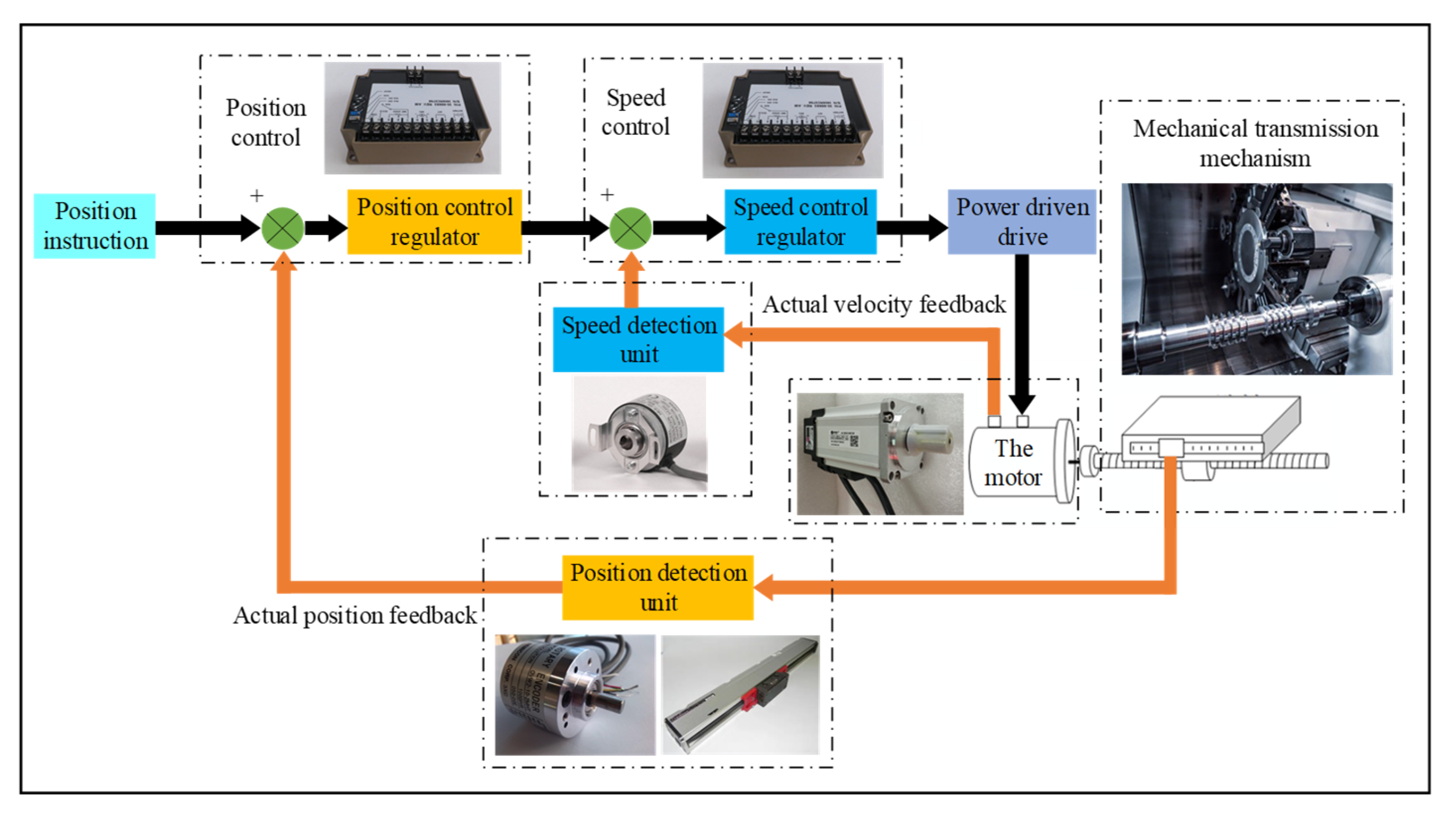
The CNC machine tool servo system mainly includes a feed servo system and spindle servo system, and Figure 2 shows its composition and workflow diagram. The feed servo system operates mainly through the numerical control system to transmit information and control the movement of the device to achieve the speed control of feed movement, while accurately controlling the moving position of the workpiece. The CNC machine tool spindle feed servo system includes a servo motor and servo drive device in two parts, of which the spindle feed servo system is connected to the speed control system, with speed control function and positive and negative rotation function. The speed control range is wide, controlled by the CNC device, and can also be controlled by a programmable controller. At present, the common spindle feed servo system includes a DC spindle control system and AC spindle control system, and the fault types are also significantly different.

2.2. Failure Data Analysis of CNC System

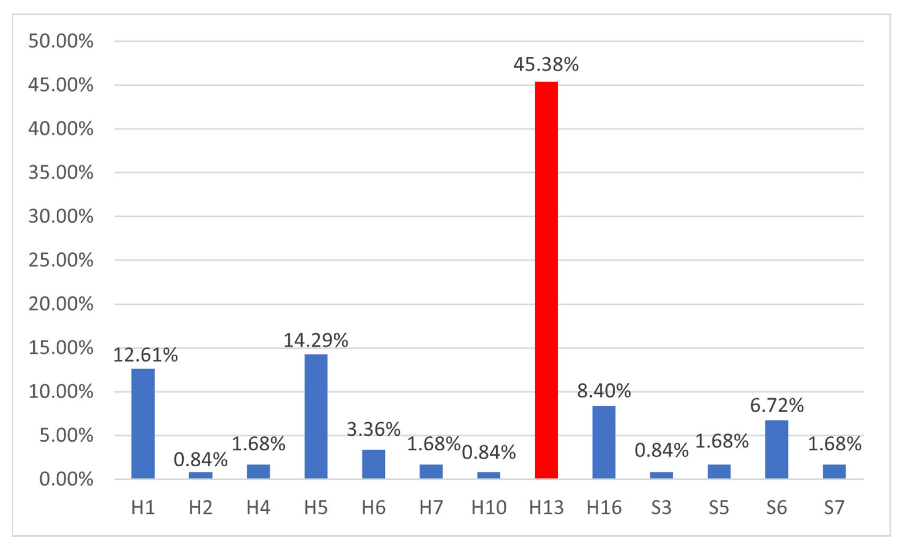
The fault analysis of a certain type of high-grade numerical control system is carried out. The fault data of the CNC machine tool with this type of CNC system are tracked and recorded for three years, and the fault data related to the CNC system are extracted from the obtained data. According to the division of function modules and faulty parts, the faulty parts of the numerical control system are statistically analyzed. The number and frequency of failures in each faulty part are shown in

Table 1. Number and frequency of faulty parts of CNC system.

Code	Position	Times	Frequency
H1	Motherboard	15	12.61%
H2	CPU	1	0.84%
H4	RAM	2	1.68%
H5	Power Supply	17	14.29%
H6	CNC Panel	4	3.36%
H7	Machine Operation Panel	2	1.68%
H10	Manual Box	1	0.84%
H13	Feed Servo System	54	45.38%
H16	Electrical System	10	8.4%
S3	Preprocessing Module	1	0.84%
S5	Position Control Module	2	1.68%
S6	PLC Software Module	8	6.72%
S7	Real-Time Management Module	2	1.68%

and Figure 3.

From the statistical data, the most common part in CNC system failure is the feed drive unit, and its failure frequency is much higher that of than other parts. This shows that the servo drive system is the main component affecting the stability of the machine tool but also the key to improve its reliability.

2.3. Fault Analysis of Feed and Spindle Servo System

The fault types of CNC machine tools are diverse, including feed system, spindle servo system and auxiliary mechanism, and other parts, and any link problems will affect the normal operation of CNC machine tools. In practical applications, the servo system of CNC machine tools has a high probability of failure. Some faults can be displayed through the CRT or the operation panel alarm, some can be displayed using the hardware display on the servo unit, and some only show that the feed movement is abnormal, but there is no warning information, so such faults are more difficult to judge and bring great difficulty for subsequent maintenance and management work. In such a complex situation, it is of great significance to predict, diagnose, and eliminate various faults quickly and accurately to improve the production efficiency and machining accuracy of the machine tool.

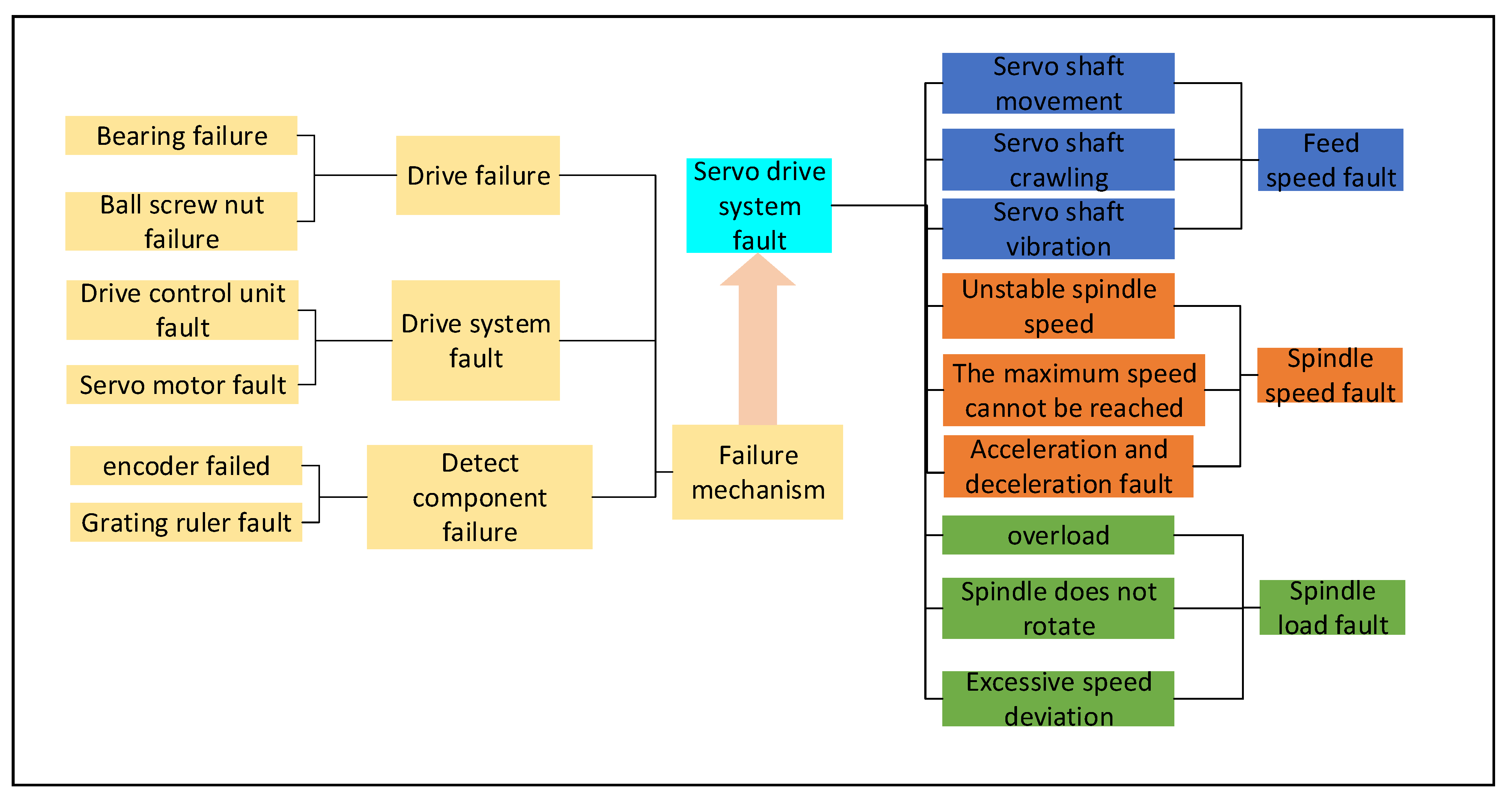
To determine and eliminate the system fault timely and accurately, a comprehensive overview of the common fault types of the existing servo drive system is made, and its fault mechanism is deeply analyzed, as shown in Figure 4. The types of fault that occur in the servo system can include the servo shaft moving, the spindle speed becoming unstable, being unable to reach the highest speed, acceleration and deceleration failure, speed deviation being too large, etc. Some of the reasons for these failures are analyzed as follows:

Servo shaft moving: feed transmission chain has reverse clearance, servo drive gain is too large.

Servo shaft crawling: servo system gain is too low, poor lubrication of the feed transmission chain, etc.

Servo shaft vibration: the bearing of the motor is poorly lubricated, the fastening screw inside the motor is loose, etc.

The spindle speed is unstable: the tachometer generator installed at the tail of the spindle fails, the speed command voltage is poor or wrong, etc.

Cannot reach the highest speed: motor excitation current adjustment is too large, the excitation control loop is bad.

Acceleration and deceleration failure: current feedback loop setting, mechanical transmission system is poor.

Overload: excessive load, poor lubrication of the feed transmission chain, etc.

Spindle does not turn: machine load is too large, mechanical connection falls off, etc.

Excessive speed deviation: improper adjustment of setting of speed regulator or speed measurement feedback loop, etc.

The root cause of servo drive failure is explored, and it is found that it is related to the transmission device, drive system, and detection components of the machine tool. When the transmission device fails, the power of the motor and other devices cannot be transferred to the actuator, and the failure mostly occurs in the coupling, lead screw, bearing, machine tool guide, and other parts. The drive system refers to the servo motor and other driving devices, and the failure of the drive system mainly includes the failure of the drive control unit and the servo motor. The detection parts mainly include the encoder, grating ruler, and other detection parts, and the fault of the detection part is mainly manifested as the feedback data error being too large or no feedback.

The faults of the servo drive system mentioned in the above analysis can be classified into three categories according to the fault nature: feed speed fault, spindle speed fault, and spindle load fault. In the case of complex fault causes, the accurate identification of the fault category can provide help for the subsequent determination of the fault location and the formulation of maintenance plans, which is of great significance to ensure the production reliability and efficiency of CNC machine tools.

3. Method

3.1. Basic Theory and Techniques for LSTM

The LSTM neural network is a special kind of recurrent neural network (RNN), which has a wide range of applications in sequence data processing and timing prediction tasks [41]. Compared with traditional RNNs, LSTM solves the problem of gradient disappearance and gradient explosion in traditional RNNs by introducing a long short-term memory unit, making it better able to capture long-term dependencies.

The core idea of the LSTM network is to control the flow of information and the update of memory by a gating mechanism. Each LSTM unit contains an input gate, a forget gate, an output gate, and a memory unit, which control the weights of input, forgetting, and output. The input gate determines the weight of the new input, the forget gate determines the degree of retention of the memory unit at the previous moment, the output gate determines the weight of the output, and the memory unit is responsible for storing and transmitting information.

The flexibility of the LSTM through the gating mechanism enables it to adaptively and selectively ignore or retain information in the input data, thus better capturing long-term dependencies in the sequence. In addition, LSTM also has trainable parameters that can be trained end-to-end using backpropagation algorithms. By training on a large amount of data, LSTM can learn patterns and regularities in the data to achieve predictions of future time series data. At the same time, LSTM can also build a deeper neural network model by stacking multiple LSTM layers or combining with other neural network layers to improve the expressiveness and performance of the model.

3.1.1. LSTM Algorithm Flow

LSTM cell structure is shown in Figure 5. LSTM uses two gates to control the content of cell state c, one is the forget gate, which determines how much of the cell state $c_{t-1}$ at the previous time is retained to the current time ${\mathrm{c}}_{\mathrm{t}}$. The other is the input gate, which determines how much of the network’s input $x_t$ is saved to the cell state ${\mathrm{c}}_{\mathrm{t}}$ at the current moment. LSTM uses an output gate to control how much of the ${\mathrm{c}}_{\mathrm{t}}$ state of the unit is output to the LSTM’s current output value ${\mathrm{h}}_{\mathrm{t}}$.

$$\mathrm{Forgotten} \mathrm{gate}:f_t=\sigma \left({\mathit{W}}_{\mathit{f}}\cdot \left[h_{t-1},x_t\right]+b_f\right),$$

(1)

In the above formula, ${\mathit{W}}_{\mathit{f}}$ is the weight matrix of the forget gate, $\left[h_{t-1},x_t\right]$ represents joining two vectors into a longer vector, $b_f$ is the bias term of the forget gate, and $\sigma$ is the sigmoid function. If the dimension of the input is ${\mathrm{d}}_{\mathrm{x}}$, the dimension of the hidden layer is ${\mathrm{d}}_{\mathrm{h}}$, and the dimension of the cell state is ${\mathrm{d}}_{\mathrm{c}}$ (usually ${d_c=\mathrm{d}}_{\mathrm{h}}$), then the dimension of the weight matrix ${\mathit{W}}_{\mathit{f}}$ of the forget gate is $d_c\times ({\mathrm{d}}_{\mathrm{h}}+d_x)$. In fact, the weight matrix ${\mathit{W}}_{\mathit{f}}$ is a concatenation of two matrices: one is ${\mathit{W}}_{\mathit{f}\mathit{h}}$, which corresponds to the input $h_{t-1}$, whose dimension is $d_c\times {\mathrm{d}}_{\mathrm{h}}$. The other is ${\mathit{W}}_{\mathit{f}\mathit{x}}$, which corresponds to the input $x_t$, whose dimension is $d_c\times {\mathrm{d}}_{\mathrm{x}}$. ${\mathit{W}}_{\mathit{f}}$ can be written as:

$$\left[{\mathit{W}}_{\mathit{f}}\right]\left[\begin{array}{c}{h}_{t-1}\\ x_t\end{array}\right]=\left[\begin{array}{cc}{\mathit{W}}_{\mathit{f}\mathit{h}}& {\mathit{W}}_{\mathit{f}\mathit{x}}\end{array}\right]\left[\begin{array}{c}{h}_{t-1}\\ x_t\end{array}\right]={\mathit{W}}_{\mathit{f}\mathit{h}}{h}_{t-1}+{\mathit{W}}_{\mathit{f}\mathit{x}}{x}_t,$$

(2)

$$\mathrm{Input} \mathrm{gate}:i_t=\sigma (W_i\cdot [h_{t-1},x_t]+b_i),$$

(3)

In the above formula, $W_i$ is the weight matrix of the input gate and $b_i$ is the offset term of the input gate.

$\widetilde{c_t}$ is used to describe the cell state of the current input, which is calculated based on the last output and the current input:

$$\widetilde{c_t}=tanh\left(W_c\cdot \left[h_{t-1},x_t\right]+b_c\right),$$

(4)

$c_t$ is the state of the cell at the current time. It is produced by multiplying the previous cell state $c_{t-1}$ by element by the forget gate $f_t$, then multiplying the current input cell state $\widetilde{c_t}$ by element by the input gate $i_t$, and adding the two products:

$$c_t=f_t\circ c_{t-1}+i_t\circ \widetilde{c_t},$$

(5)

The symbol $\circ$ means multiplication by element.

LSTM can combine the current memory $\widetilde{c_t}$ with the long-term memory $c_{t-1}$ to form the new cell state $c_t$. Thanks to the control of the forget door, it can save information from a long time ago, and because of the control of the input door, it can avoid the current insignificant content in the memory.

$$\mathrm{Output} \mathrm{gate}:o_t=\sigma (W_o\cdot [h_{t-1},x_t]+b_o),$$

(6)

The final output of the LSTM is determined by the output gate and the cell state:

$$\mathrm{Output}: h_t=o_t\circ tanh\left(c_t\right),$$

(7)

Table 2. Activation function description.

The Activation Function	The Formula
Sigmoid	$Sigmoid\left(x\right)=\frac{1}{1+e^{-x}}$
TanH	$Tanh\left(x\right)=\frac{e^x-e^{-x}}{e^x+e^{-x}}$

shows the formula of the activation function.

3.1.2. Drawbacks of the LSTM Method

When there are enough sample data, LSTM can perform the prediction task based on time series well. However, LSTM also has some defects in time series forecasting:

(1) LSTM has a relatively complex structure, including more gating units and memory units, which may lead to higher model complexity. This results in LSTM being computationally more complex, requiring more computational resources and time for training and reasoning, while being more prone to overfitting, requiring more data to generalize and improve performance.

(2) Because LSTM has more parameters and a more complex structure, it may require longer training time and more data to converge and achieve optimal performance. In addition, the LSTM training process is also more prone to gradient disappearance or explosion problems, and skill is needed to alleviate these problems.

(3) The complexity and number of parameters of the LSTM may lead to an increased risk of overfitting. In a timing prediction task, overfitting can result in a model that performs well on training data but poorly on previously unseen test data. Therefore, when using LSTM for timing prediction, proper regularization and model selection need to be paid attention to avoid overfitting problems.

3.2. Basic Theory and Techniques for GRU

The GRU is a variant of the RNN that uses gating mechanisms to better capture and remember long-term dependencies in sequence data [42]. There are some similarities between the GRU and the LSTM in that both have gating mechanisms that control the flow of information and the updating of memories. The main difference between them is the internal structure and the number of gating mechanisms. The GRU simplifies the structure of the LSTM and consists of only two gated units: update gate and reset gate. The update gate controls whether the memory unit from the previous moment is passed to the current moment, while the reset gate controls how the input from the current moment is combined with the memory unit from the previous moment. Because of their simpler structure and fewer parameters, GRUs can train models faster and have better computational efficiency than LSTM in some cases.

3.2.1. GRU Algorithm Flow

The GRU unit structure is shown in Figure 6. The basic flow of the GRU algorithm is as follows:

$$\mathrm{U}\mathrm{p}\mathrm{d}\mathrm{a}\mathrm{t}\mathrm{e} \mathrm{g}\mathrm{a}\mathrm{t}\mathrm{e}:z_t=\sigma (w_z\cdot [h_{t-1},x_t\left]\right)$$

(8)

$${\mathrm{R}\mathrm{e}\mathrm{s}\mathrm{e}\mathrm{t} \mathrm{g}\mathrm{a}\mathrm{t}\mathrm{e}:r}_t=\sigma (w_r\cdot [h_{t-1},x_t\left]\right)$$

(9)

The reset gate is used to decide how to merge the hidden state of the previous moment with the input of the current moment, and the update gate is used to decide whether to pass the hidden state of the previous moment to the current moment.

Calculation of candidate hidden state of GRU:

$$\widetilde{h_t}=tanh(w_h\cdot [r_t⨀h_{t-1},x_t\left]\right)$$

(10)

where ⊙ means multiplication by element.

GRU hidden status update:

$$h_t=(1-z_t)⨀h_{t-1}+z_t⨀\widetilde{h_t}$$

(11)

The final hidden state, $h_t$, will be the output at the current moment and passed to the GRU as input at the next moment.

In the above formula, $x_t$ represents the input at the current moment, $h_{t-1}$ represents the hidden state at the previous moment, $z_t$ is the update gate, $r_t$ is the reset gate, $\widetilde{h_t}$ is the candidate hidden state, and $h_t$ is the hidden state at the current moment. By iterating over the above process, the GRU can gradually update the hidden state based on the input sequence and output the corresponding hidden state at each moment. This allows the GRU to effectively capture long-term dependencies in sequence data, suitable for tasks such as natural language processing, time series prediction, and more.

3.2.2. Limitations of GRU Method in Failure Prediction

As a common recurrent neural network, the GRU is often used for timing processing tasks, and although the GRU performs well in many sequence modeling tasks, there are still some limitations in fault prediction:

(1) Long-term dependence: Although the GRU solves the problem of gradient disappearance or explosion in the traditional circulating neuron through the gating mechanism, there are still limitations in the modeling of long-term dependence. In failure prediction, some failures may be caused by complex factors over a long period of time in the past, and the GRU may not be able to effectively capture this long-term dependence.

(2) Difficulty in parameter adjustment: Many parameters in the GRU model need to be adjusted, including learning rate, regularization, etc. In fault prediction, the selection of these parameters may be affected by factors such as data quality, sample size, and fault type, so adjustments need to be made, increasing the difficulty of modeling.

3.3. Basic Theory and Techniques for SOM

SOM is an unsupervised neural network, which effectively retains the original topology of input samples in an intuitive visual form, and is an important tool for fault diagnosis and monitoring [43]. SOM employs competitive learning, in which each neuron or node competes with other nodes or neurons to get closer to the input data point. Finally, the network is formed by clustering and grouping similar input data points together. As a kind of unsupervised learning competitive neural network, SOM has good topological relationship preservation performance and strong self-learning ability and has great advantages in visualization, so it is widely used in the field of cluster analysis.

SOM consists of a grid map and a low-dimensional matrix, with each node considered to be a neuron. The neurons in the network each have a weight vector the same size as any input data point. This matrix is used to evaluate the distance of any input vector from each cell weight in the data set. In the initialization phase, the weights of each cell are randomly assigned, and then the data points find the closest neuron and are assigned to the nearest neuron. The neuron with the smallest distance can be called the best matched unit (BMU). The weight of the BMU is then updated as neurons move towards the data point. During the same iteration, the weights of neurons adjacent to the BMU are also updated so that they move in the same direction as the displaced BMU, but at a lower rate. As more iterations are made during the training process, the amount of change in the neuron weights decreases as the grid map gradually approaches the input data points with each iteration. All data points in the training process are ongoing. After the network training is complete, each data point is assigned to a cell of the grid map. Inputs with similar data characteristics are grouped around adjacent cells, and SOM networks are often constructed as two-dimensional, regularly arranged lattice arrays of neurons, as shown in Figure 7.

3.3.1. SOM Algorithm Flow

The SOM neural network obtains the winning node by outputting neurons in the competition layer, and the weight of the connection between the winning neuron and the input layer needs to be changed. The weight value is changed to make the difference between the input variable and the winning neuron smaller and smaller, so that similar input variables are like the weight of the output neuron connection, and similar input variables are clustered into the same class.

The specific algorithm steps are as follows:

(1) Initialize

Set the initial value of learning rate $\alpha \left(0\right)$, the initial value of neighborhood radius $r\left(0\right)$, and the neuron weight vector $w_{ii}$.

(2) Look for winning neurons

Calculate the distance $d_j$ between the input vector and the output neuron to find the winning neuron.

$${\mathrm{d}}_{\mathrm{j}}=\sqrt{{\sum }_{\mathrm{i}=1}^{\mathrm{m}}{(x_{\mathrm{i}}-w_{\mathrm{i}\mathrm{j}})}^2},$$

(12)

where ${\mathrm{X}}_{\mathrm{i}}$ is the selected vector; ${\mathrm{W}}_{\mathrm{i}\mathrm{j}}$ is the weight of the ith neuron in the input layer and the jth neuron in the output layer. The one with the smallest distance is the winning neuron. The neuron satisfies Equation (10).

$$\mathrm{s}\left(\mathrm{i}\right)=\arg \mathrm{m}\mathrm{i}\mathrm{n}\left|\right|x_{\mathrm{i}}-w_{\mathrm{i}\mathrm{j}}\left|\right|$$

(13)

(3) Update weights

The weight of the winning neuron within the radius of the neighborhood is updated, and the learning adjustment of the weight vector is shown in Equations (11) and (12).

$$w\left(\mathrm{t}\right)=w\left(\mathrm{t}-1\right)+\alpha \left(\mathrm{t}\right)\mathrm{A}\left(x_{\mathrm{i}}-w_{\mathrm{j}}\right),$$

(14)

$$\mathrm{A}=\left\{\begin{array}{c}1, \mathrm{c}=\mathrm{q}\\ 0.5, \mathrm{c}\in {\mathrm{r}}_{\mathrm{q}}\left(\mathrm{t}\right)\\ 0, \mathrm{others} \end{array}\right.,$$

(15)

Where c represents neurons in the output layer; q is the winning neuron; $r_q\left(t\right)$ is the winning neighborhood.

(4) Update learning rate and neighborhood radius

$$\eta \left(\mathrm{t}\right)=\left(1-t/\mathrm{T}\right)\times \mathsf{\eta }\left(0\right),$$

(16)

$$r\left(\mathrm{t}\right)=\left(1-t/\mathrm{T}\right)\times \mathrm{r}\left(0\right),$$

(17)

(5) Judge whether the training times reach the preset value and, if so, end the training; otherwise continue training.

3.3.2. Limitations of SOM Method in Fault Diagnosis

As a clustering and visualization algorithm, SOM is commonly used in the field of fault diagnosis. However, due to the performance limitations of SOM itself, there are some limitations in handling fault diagnosis tasks, especially when dealing with large data samples and high-dimensional data:

(1) Data volume limitation: The SOM method has certain limitations when dealing with large-scale data. The data sample size of the fault diagnosis task is large, and the SOM method needs more iterations to converge to a stable result, which increases the calculation time and cost. Meanwhile, the SOM method may be affected by data sampling and distribution, resulting in increased instability of model training results.

(2) Data dimension limitation: The SOM method has limited processing capacity for high-dimensional data. SOM has a good clustering effect when processing low-dimensional data, but when performing fault diagnosis tasks, the data dimensions are high, and the mapped results may lose some feature information of the original data, resulting in errors in the identification of cluster centers and aliasing.

4. Proposed Method

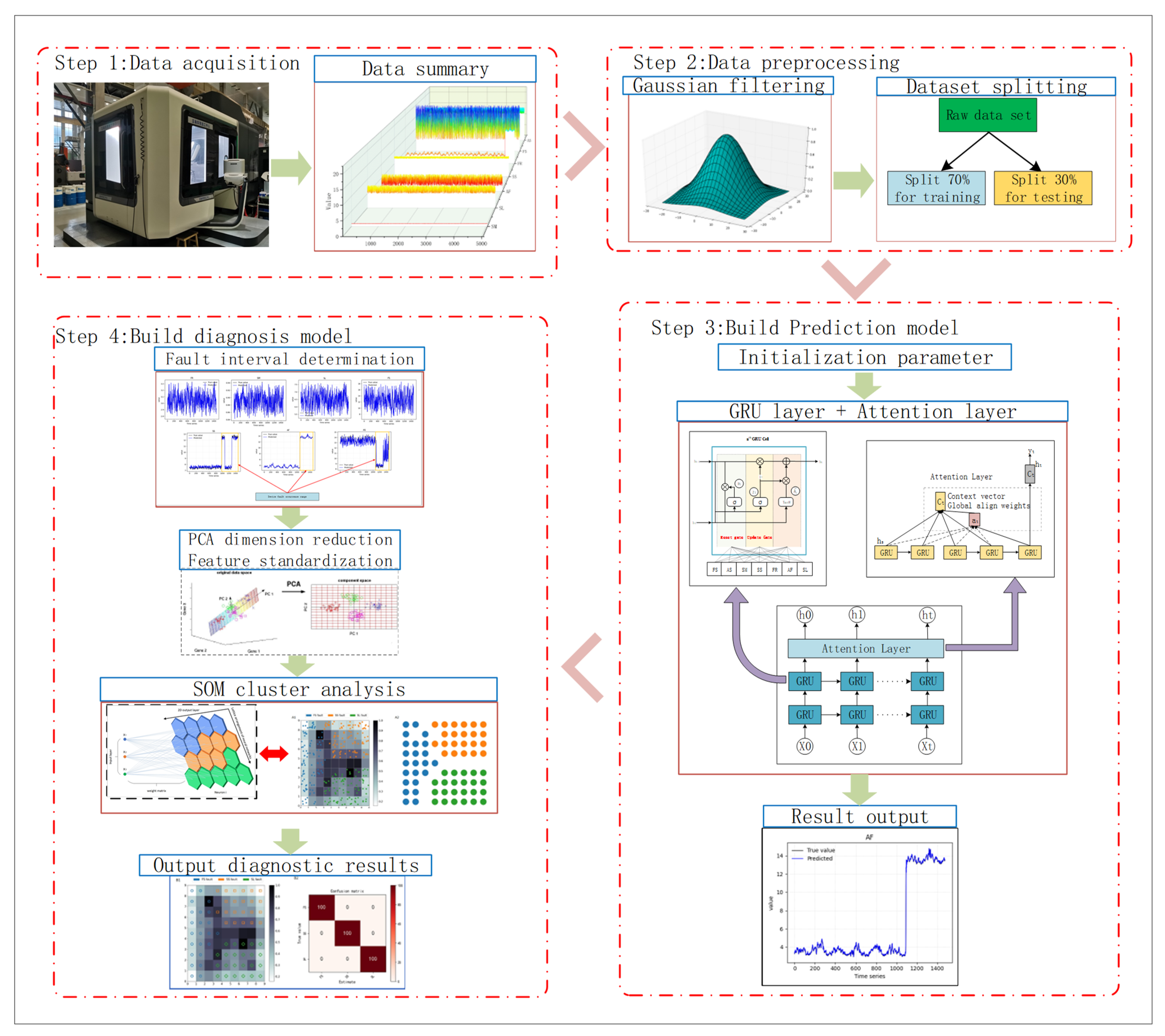
4.1. Health Management Process Based on Attention-MLGRU and PCA-SOM Algorithms

To ensure the normal operation of a CNC machine tool servo drive system for a long time, a health management method of a machine tool servo drive system based on the Attention-MLGRU and PCA-SOM algorithms was proposed. The core of this method includes two parts, fault prediction and fault diagnosis. In the fault prediction stage, a multi-layer GRU neural network is used to predict the time sequence of the operating parameters, and the attention mechanism is introduced to establish the fault prediction model of the servo drive system. The introduction of the attention mechanism in GRU neural networks can improve the long-term dependence problem of GRU neural networks, improve model performance, handle variable-length input sequences, and provide interpretability and interpretability. This makes the model more flexible, accurate, and interpretable in sequence tasks.

In the fault diagnosis stage, the SOM neural network is used for cluster analysis, and feature standardization and PCA are introduced into the SOM neural network to establish the fault diagnosis model of the servo drive system. The fault diagnosis effect of the model is better than that of the traditional method, and it can realize the dimensionality reduction analysis of high-dimensional fault data and can accurately identify the fault characteristics of the data, which solves the problem that the fault causes of the existing CNC machine tool servo drive control system are complicated and difficult to diagnose and provides a good idea for the fault diagnosis of the CNC machine tool servo drive system and improves the operation reliability of the machine tool. The specific process of health management is shown in Figure 8.

Step 1: Use the workshop detailed manufacturing data and process system (MDC system) to monitor the actual production status of CNC machine tools and collect data for some key production parameters.

Step 2: According to the production data of the field equipment of the MDC system, select appropriate data as the sample data set and conduct data preprocessing. The data preprocessing adopts the Gaussian filter method, and the processed data set is used as the input for fault prediction and fault diagnosis analysis.

Step 3: Fault prediction

(1) Initialization of parameters: Initialize the weight and bias of the multi-layer GRU neural network.

(2) Forward propagation: For each time step, calculate the current input and the hidden state of the previous time step, as well as the attention weight. The input sequence is weighted and summed according to the attention weight to obtain the attention-weighted representation. The attention-weighted representation is input into a multi-layer GRU, and the hidden state of the current time step is calculated.

(3) Calculate the loss: Input the hidden state of the last time step into the output layer, calculate the predicted value, and calculate the loss function according to the predicted value and the target label.

(4) Backpropagation: Calculate the gradient of the loss function to the predicted value and calculate the gradient of each parameter in the multi-layer GRU neural network through the backpropagation algorithm.

(5) Use the Nadam algorithm to update network parameters, adjust weights and bias.

Step 4: Fault diagnosis

(1) Carry out feature standardization processing for different types of input sample data sets and determine the parameters of the output layer.

(2) Establish an improved self-organizing neural network fault diagnosis model, input the feature standardized sample data set into the model, and conduct PCA dimensionality reduction to obtain the sample data after dimensionality reduction.

(3) Conduct SOM cluster analysis on the sample data after dimensionality reduction and output the cluster analysis results.

(4) Output fault diagnosis results according to cluster analysis results and determine the fault diagnosis accuracy rate.

4.2. Instructions on Data Set Creation

4.2.1. Potential Challenges in Data Set Creation

In the construction of a health management system, data are crucial, and given the reality of production, the establishment of data sets faces some potential challenges and limitations:

(1) Difficulty in obtaining data: Generally speaking, the data required for fault prediction and diagnosis may need to be obtained from multiple sources, including equipment logs, maintenance records, etc. There may be difficulties in obtaining these data at the same time, such as data access restrictions, data integration problems between devices and systems, etc., so appropriate ways are needed to obtain relevant data.

(2) Insufficient amount of data: The establishment of an effective fault prediction and diagnosis model usually requires a large amount of data to train, especially for the diagnosis of complex systems and multiple types of faults. In actual production, there may be an insufficient volume of data, which affects the performance and generalization ability of the model.

(3) Poor data quality: the actually collected data may have quality problems, such as outliers, noise, etc., which may affect the training and prediction accuracy of the model, so it is necessary to clean and preprocess the acquired data in an appropriate way to ensure the quality of the data set.

4.2.2. MDC System Overview

Intelligent monitoring plays an important role in the intelligent automation of manufacturing systems, and advanced data collection technology has been widely used to promote real-time data collection [44]. The Manufacturing Data Collection & Status Management (MDC) system is a software and hardware solution for real-time acquisition, charting, and reporting of detailed manufacturing processes and data on the shop floor. MDC uses a variety of flexible methods to obtain real-time data from the production site (including equipment, people, production tasks, etc.), store it in databases such as Access, SQL, and Oracle, and build on the lean manufacturing management philosophy. Combined with nearly 100 kinds of special calculation, analysis, and statistical methods of the system, it directly reflects the production status of the workshop in the form of a variety of reports and charts and helps the production department of the enterprise to make scientific and effective decisions. Figure 9 is the MDC system diagram.

The MDC system has the following characteristics when processing data:

(1) Real-time data acquisition: The MDC system can collect all kinds of data in the production process in real time, including equipment operation data, sensor data, etc. Compared with traditional data acquisition methods, the MDC system has the characteristics of automation and real time, which can greatly improve the efficiency and accuracy of data acquisition.

(2) Data consistency: By automating data collection and processing, the MDC system ensures data consistency and accuracy, avoiding errors and inconsistencies caused by manual operations and ensuring data reliability and availability.

(3) Historical data recording: The MDC system can record and store historical data to form a complete historical data record to ensure the integrity and quantity of data, which is important for fault analysis and the fault prediction model.

Using the MDC system to obtain data ensures data availability and quantity requirements are met.

4.2.3. Data Preprocessing Method—Gaussian Filter

Gaussian data filtering is a common signal processing technique used to reduce high-frequency noise in data, smooth data, and retain low-frequency information in data. Its principle is based on the characteristics of the Gaussian function, by weighted average data to achieve filtering.

The Gaussian function is a continuous distribution function in the shape of a bell curve. In data filtering, the Gaussian function is used as the convolution kernel of the filter. The convolution kernel is the core function of weighted summation of input data, smoothing input data, and reducing noise in the data. In Gaussian data filtering, the convolution kernel is determined by a standard deviation parameter. The higher the standard deviation, the higher the smoothing degree of the filter and the better the filtering effect of the data noise. In the filtering process, each point in the convolution checks data and its adjacent points are weighted to calculate the filtering value of the point.

By using Gaussian filtering, the high-frequency noise in the data can be removed to smooth the data, while retaining the low-frequency information in the data, improving the quality and accuracy of the data, so as to ensure the data quality of the data set.

4.2.4. Introduction to Data Characteristics

The MDC system is used to collect the actual running data of CNC machine tools, and some working parameters that can characterize the running state of the machine tools are analyzed, including feed speed, actual speed, spindle ratio, spindle speed, feed rate, actual feed, and spindle load, as shown in

Table 3. Equipment parameter type.

Device Parameter Type	The Symbol	Device Parameter Type	The Symbol
Feed speed	FS	Feed rate	FR
Actual speed	AS	Actual feed	AF
Spindle magnification	SM	Spindle load	SL
Spindle speed	SS	Label	LA

.

According to the seven field equipment production data collected by the MDC system, data are selected as a sample data set at a certain time interval and taken as input, as shown in

Table 4. Equipment fault types and corresponding indicators.

The Fault Types	On the Limit	Under the Limit	Ideal Value	Unit
Feed speed fault	20 × 10−3	5 × 10−3	18.8 × 10−3	in/r
Actual speed fault	15	12	13.5	in/r
Spindle magnification fault	0.95	0.83	0.89	%
Spindle speed fault	8 × 103	7 × 103	7.5 × 103	r/min
Feed rate fault	3.4	2.7	3.2	mm/r
Actual feed fault	6.5	2	4.7	mm/r
Spindle load fault	8	5	5.3	%

, which includes three types of fault data that can characterize the servo drive system, including feed speed, spindle speed, and spindle load. Three types of trouble-free data, including actual speed, spindle rate feed, and actual feed are included. The label value indicates the fault type of the data sample, where “1” indicates the feed speed fault, “2” indicates the spindle speed fault, and “3” indicates the spindle load fault. Table 4 shows the fault indicators of each fault type. When the working parameters are within the target range, the servo drive system is in a normal working state; when the working parameters are beyond the target range, the corresponding fault occurs. A waterfall diagram of the running parameters of the machine tool is shown in Figure 10.

4.3. Fault Prediction Method

4.3.1. Attention Mechanism Principle

The attention mechanism is a mechanism for weighting information at different locations in the sequence data [45]. The introduction of the attention mechanism in the neural network model allows the model to make different attention adjustments to the input at different moments when processing the sequence data so that the key information in the sequence can be processed more flexibly. The structure of the attention mechanism is shown in Figure 11.

The formula expression of the attention mechanism can vary according to the specific variant. The following is a general formula expression of the attention mechanism:

Given the input sequence $H=(h_1$, $h_2$,……, $h_t)$, the attention mechanism calculates the attention weight\alpha and the context vector c as follows:

1. Calculate attention weight:

$${ \alpha }_i=\frac{exp\left(e_i\right)}{{\sum }_{i=1}^{T}exp\left(e_j\right)}$$

where $e_i$ is the result of the score function score, which measures the correlation of position i with other positions in the sequence.

2. Calculate the context vector:

$$c={\sum }_{i=1}^T{\mathsf{\alpha }}_{\mathrm{i}}{\mathrm{h}}_{\mathrm{i}}$$

In the self-attention mechanism, the common scoring function score has the following forms:

Product attention: $e_i=h_i\cdot h_i$;

Additive attention: $e_i=tanh\left(W_x{h}_i+b\right)$;

Where $W_x$ is a learnable weight matrix and b is a learnable bias vector.

Scaled dot product attention: $e_i=\frac{h_i\cdot h_i}{\sqrt{d}}$;

Where d is the dimension of the input sequence.

The above formula is the general form of the attention mechanism, and the specific application scenario and model will determine the appropriate scoring function and calculation method.

The introduction of attention mechanisms in neural networks can improve the long-term dependency problem of LSTM and GRU neural networks, improve model performance, handle variable-length input sequences, and provide interpretability and explainability. This makes the model more flexible, accurate, and interpretable in sequence tasks.

4.3.2. Type of Neural Network Structure

In general, neural network structures come in many variants, including single-layer, multi-layer, and bidirectional neural network structures. In general, a single-layer neural network has a simple structure and high computational efficiency, but its learning ability is limited. A multi-layer neural network has stronger representation and learning ability, which is suitable for various complex tasks. A bidirectional neural network can make use of bidirectional dependency to provide more comprehensive context information when processing sequence data. Choosing a suitable neural network structure depends on the complexity of the task and the characteristics of the data.

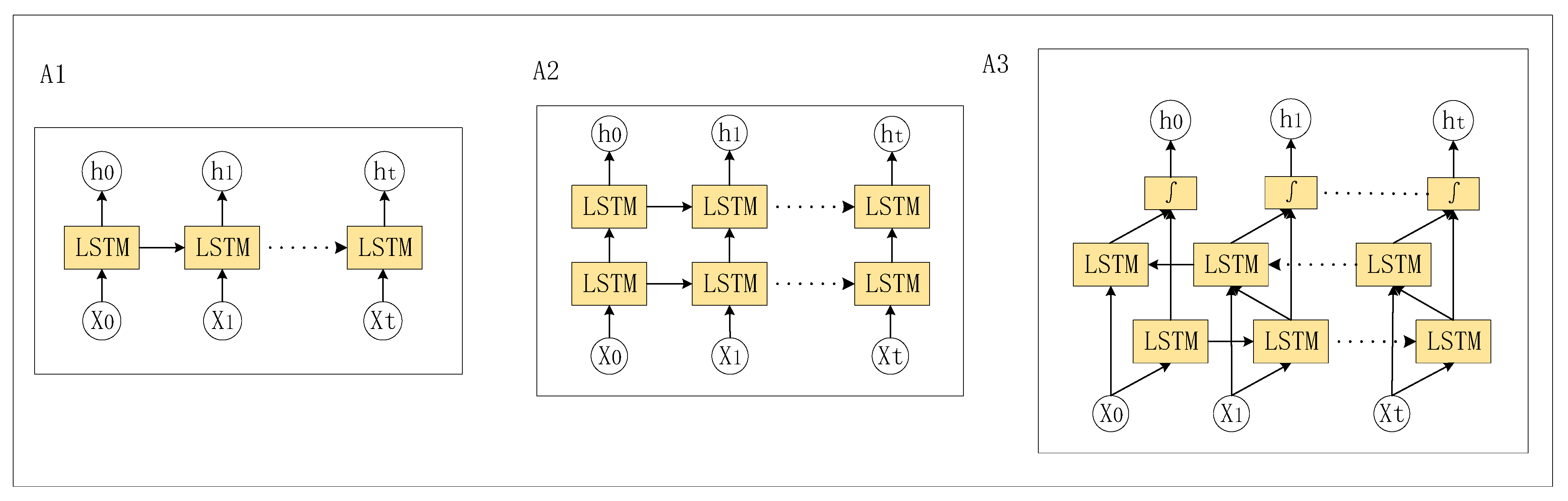
Several variants of the LSTM structure are shown in Figure 12, including:

1. Single-layer LSTM: Also known as standard LSTM, it contains three gate control units (input gate, forget gate, and output gate), as well as a memory unit (cell state), which can conduct long-term dependency modeling of sequence data.

2. Multi-layer LSTM: A network structure composed of multiple LSTM layers. Each LSTM layer can obtain input from the output of the previous layer and increase the complexity and representation of the model by stacking multiple LSTM units.

3. Bidirectional LSTM: Based on the standard LSTM, the forward and reverse LSTM units are introduced, which can model the sequence data in both forward and backward directions at the same time to capture more comprehensive context information.

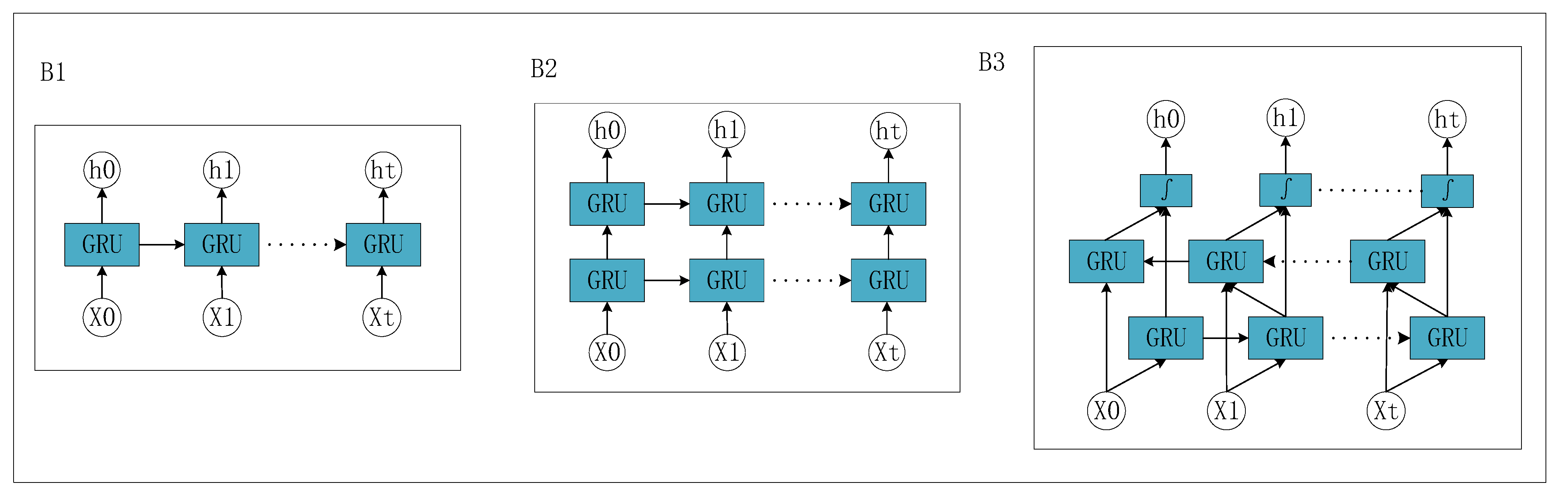
Several variations of the GRU structure are shown in Figure 13, including:

1. Single-layer GRU neural network: The single-layer GRU neural network contains only one GRU hidden layer and, compared with LSTM, the GRU has a more simplified structure, reducing a part of the gating unit, and the number of calculations and parameters is lower. Single-layer GRUs show better performance when dealing with simple sequential tasks. The training speed is relatively fast, which is suitable for medium-scale data sets.

2. Multi-layer GRU neural network: The multi-layer GRU neural network contains multiple GRU hidden layers, and the output of the upper layer serves as the input of the next layer. The multi-layer structure can capture more complex sequence patterns and abstract representations, while increasing the depth and expressiveness of the network. It is suitable for processing more complex sequences, but the complexity of training and parameter adjustment is higher. More computing resources and more data are needed to avoid overfitting.

3. Bidirectional GRU neural networks: Bidirectional GRU neural networks consider both past and future contextual information. At each time step, the input sequence is passed forward and backward to the two GRU hidden layers, and their outputs are merged. Bidirectional architecture can better capture dependencies and context information in sequence data and is suitable for sequential tasks such as speech recognition, machine translation, etc., but the training time and computing resource consumption are relatively high.

Choosing a single-layer, multi-layer, or bidirectional neural network architecture requires trade-offs based on the specific task and complexity of the data set, as well as training time and computational resource constraints. The LSTM and GRU neural network structures with an attention mechanism are shown in Figure 14 and Figure 15.

4.3.3. Attention-MLGRU Algorithm Flow

The attention-based multi-layer GRU neural network is a recursive neural network structure that combines attention mechanisms for processing sequence data. By introducing attention mechanisms, it can automatically learn and focus on key information in the input sequence.

1. Forward propagation:

It is assumed that there is a multi-layer GRU network with an L-layer, and the attention mechanism is introduced. The calculation process of each GRU unit can be expressed as:

The reset gate of the GRU unit on level l:

$${\mathrm{r}}_{\mathrm{t}}^{\left(\mathrm{l}\right)}=\mathsf{\sigma }({\mathrm{W}}_{\mathrm{r}}^{\left(\mathrm{l}\right)}{\mathrm{x}}_{\mathrm{t}}+{\mathrm{U}}_{\mathrm{r}}^{\left(\mathrm{l}\right)}{\mathrm{h}}_{\mathrm{t}-1}^{\left(\mathrm{l}\right)}+V_r^{\left(l\right)}{c}_t+{\mathrm{b}}_{\mathrm{r}}^{\left(\mathrm{l}\right)})$$

(18)

The update gate of the GRU unit on level l:

$${\mathrm{z}}_{\mathrm{t}}^{\left(\mathrm{l}\right)}=\mathsf{\sigma }({\mathrm{W}}_{\mathrm{z}}^{\left(\mathrm{l}\right)}{\mathrm{x}}_{\mathrm{t}}+{\mathrm{U}}_{\mathrm{z}}^{\left(\mathrm{l}\right)}{\mathrm{h}}_{\mathrm{t}-1}^{\left(\mathrm{l}\right)}+V_z^{\left(l\right)}{c}_t+{\mathrm{b}}_{\mathrm{z}}^{\left(\mathrm{l}\right)})$$

(19)

The candidate hidden state of the GRU unit on level l:

$${\tilde{h}}_{\mathrm{t}}^{\left(\mathrm{l}\right)}=\mathrm{t}\mathrm{a}\mathrm{n}\mathrm{h}({\mathrm{W}}_{\mathrm{h}}^{\left(\mathrm{l}\right)}{\mathrm{x}}_{\mathrm{t}}+{\mathrm{U}}_{\mathrm{h}}^{\left(\mathrm{l}\right)}(r_t^{\left(l\right)}⨀h_{t-1}^{\left(l\right)})+V_z^{\left(l\right)}{c}_t+{\mathrm{b}}_{\mathrm{h}}^{\left(\mathrm{l}\right)})$$

(20)

where $x_t$ is the input vector, $h_{\mathrm{t}-1}^{\left(\mathrm{l}\right)}$ is the hidden state of layer l at the previous moment, ${\mathrm{r}}_{\mathrm{t}}^{\left(\mathrm{l}\right)}$ is the reset gate, ${\mathrm{z}}_{\mathrm{t}}^{\left(\mathrm{l}\right)}$ is the update gate, and ${\tilde{h}}_{\mathrm{t}}^{\left(\mathrm{l}\right)}$ is the candidate hidden state.

Calculation of attention vector:

$$e_t^{\left(l\right)}=tanh(U_a^{\left(l\right)}{h}_{t-1}^{\left(l\right)}+V_a^{\left(l\right)}{c}_t+b_a^{\left(l\right)})$$

(21)

$${\alpha }_t^{\left(l\right)}=\frac{exp\left(e_t^{\left(l\right)}\right)}{{\sum }_{j=1}^{T}exp\left(e_j^{\left(l\right)}\right)}$$

(22)

$$c_t={\sum }_{j=1}^T{\alpha }_t^{\left(l\right)}{\tilde{h}}_j^{\left(l\right)}$$

(23)

where $e_t^{\left(l\right)}$ is the intermediate result of the attention vector, ${\alpha }_t^{\left(l\right)}$ is the attention weight, $c_t$ is the attention-weighted context vector, and ${\tilde{h}}_j^{\left(l\right)}$ is the candidate always hidden state of the l-level GRU unit.

Hidden state update:

$$h_{\mathrm{t}}^{\left(\mathrm{l}\right)}=\left(1-z_t^{\left(l\right)}\right)⨀{\mathrm{h}}_{\mathrm{t}-1}^{\left(\mathrm{l}\right)}+z_t^{\left(l\right)}⨀{\tilde{h}}_t^{\left(l\right)}$$

(24)

where $h_{\mathrm{t}}^{\left(\mathrm{l}\right)}$ is the hidden state of layer l at the current moment.

The forward propagation process of the entire multi-layer GRU neural network can be expressed as:

$$h_{\mathrm{t}}^{(\mathrm{l})}={\mathrm{G}\mathrm{R}\mathrm{U}}^{\left(l\right)}(x_t,h_{t-1}^{\left(l\right)},c_t)$$

(25)

where ${\mathrm{G}\mathrm{R}\mathrm{U}}^{\left(l\right)}$ represents the GRU unit of layer l.

2. Calculate the loss function:

Use an appropriate loss function, such as the mean square error loss, to calculate the error between the predicted value and the true label.

3. Backpropagation:

According to the loss function, calculate the gradient of the loss relative to the parameter. Through the backpropagation algorithm, it is possible to calculate the gradient of the loss function to the network parameters and use the optimization algorithm (such as gradient descent) to update the parameters to train and optimize the network.

4. Parameter update (Nadam optimizer):

The Nadam optimizer uses the following formula to update parameters:

$$m_t={\beta }_1\cdot m_{t-1}+(1-{\beta }_1)\cdot g_t$$

(26)

$$v_t={\beta }_2\cdot m_{t-1}+(1-{\beta }_2)\cdot g_t$$

(27)

$${\widehat{m}}_t=\frac{m_t}{1-{\beta }_1^t}$$

(28)

$${\widehat{v}}_t=\frac{v_t}{1-{\beta }_2^t}$$

(29)

$${\theta }_t={\theta }_{t-1}-\frac{{\widehat{m}}_t}{\sqrt{{\widehat{v}}_t}+ϵ}\cdot \left({\beta }_1\cdot {\widehat{m}}_t+(1-{\beta }_1)\cdot g_t+\frac{{\beta }_1\cdot (1-{\beta }_1^{t-1})}{1-{\beta }_1^t}\cdot ({\widehat{m}}_t-m_{t-1})\right)$$

(30)

where $m_t$ and $v_t$ represent the first moment estimate and second moment estimate of the gradient, respectively, $g_t$ represents the gradient at the current moment, ${\beta }_1$ and ${\beta }_2$ are adjustable hyperparameters with a general value of 0 and 0.999, $\alpha$ denotes the learning rate, $ϵ$ is a small number (such as 1 × 10⁻⁸) used for numerical stability. $\widehat{m_t}$ and $\widehat{v_t}$ are deviation corrections for the first and second moment estimates of gradients used to solve the deviation problem of the Adam optimizer. By introducing the correction term of Nesterov momentum, the first moment estimation of the gradient is more accurate.

The weight parameters and bias terms in the above formula are updated according to the rules of gradient descent to minimize the loss function. The above steps are repeated for multiple rounds of iterative training until a predetermined stopping condition or convergence is reached. By using the attention mechanism and the Nadam optimizer, attention weights and learning rates can be adjusted adaptively in multi-layer GRU neural networks to optimize the updating process of network parameters.

4.4. Fault Diagnosis Method

4.4.1. Introduction to Principal Component Analysis

PCA is a standard method applied to reduction and feature extraction and is the most used linear dimension reduction method. The purpose of PCA for dimensionality reduction is to reduce the original features as far as possible to ensure that “information is not lost” and obtain the maximum data information (maximum variance) in the dimension of the projection. In other words, the original feature is projected onto the dimension with the maximum projection information, so that the information loss after dimensionality reduction is minimized [46] and the characteristics of more original data points are retained while the data dimension is reduced.

4.4.2. PCA-SOM Algorithm Flow

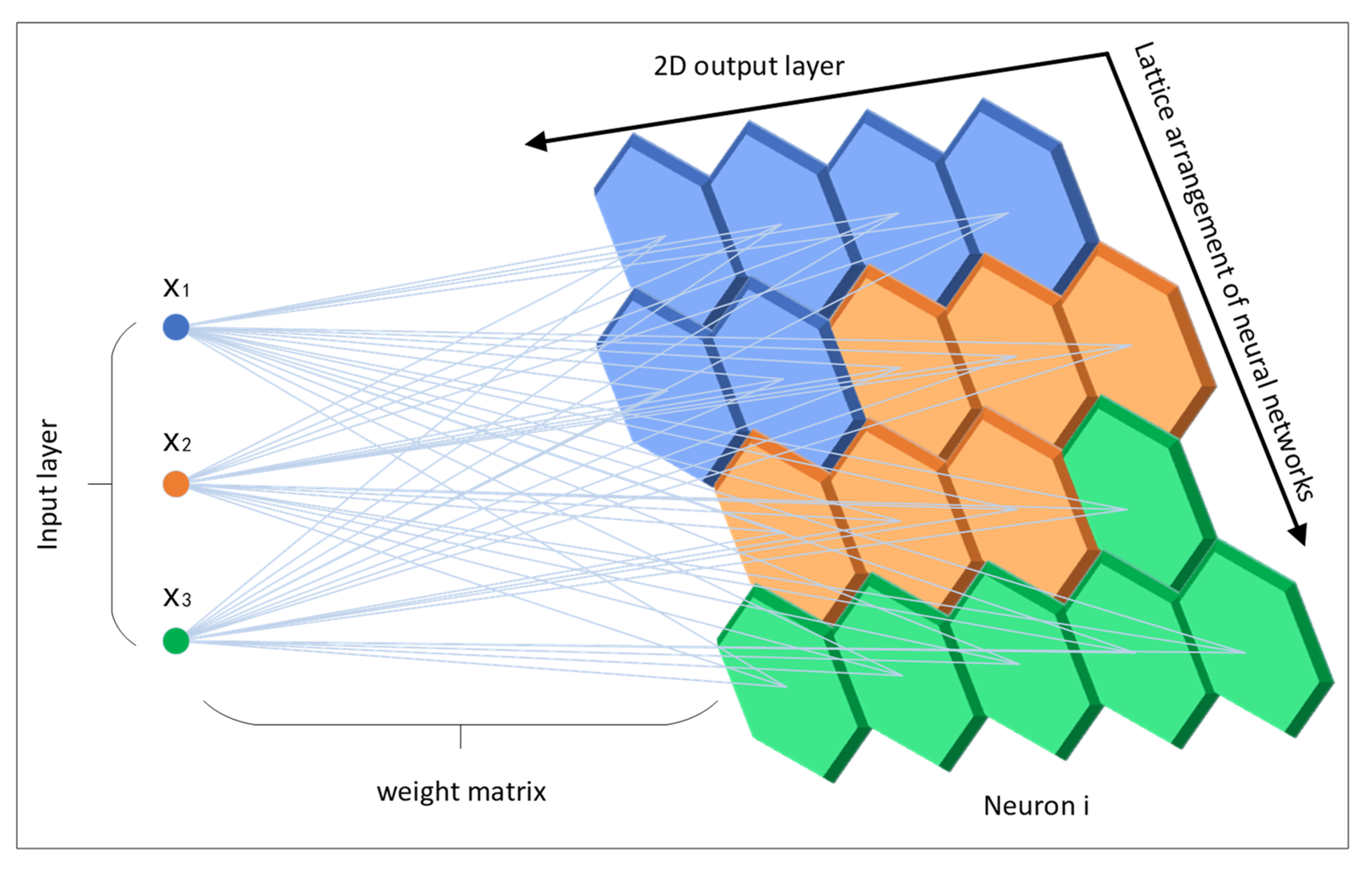
To improve the operation rate, clustering accuracy, and data processing ability of the SOM neural network, a PCA-SOM neural network is proposed by combining a PCA neural network with a SOM neural network. At the same time, feature standardization is introduced into the SOM neural network to balance the influence of different feature scales, and then the SOM neural network is further optimized. The network structure is mainly composed of an input layer and output layer. The input layer accepts high-dimensional data and transforms them into two-dimensional data visual output through a competitive learning mechanism. For the operation parameters of the equipment to be evaluated, the SOM neural network can output a two-dimensional topology after the monitoring data are processed, assuming that the number of neurons in the output layer is L. The specific algorithm process is as follows:

(1) Data feature standardization processing

Conduct feature standardization processing on the input training data matrix ${\mathit{D}}_0$, and the processed data matrix is D:

$$\mathit{D}=\frac{{\mathit{D}}_0-\mathrm{m}\mathrm{e}\mathrm{a}\mathrm{n}\left({\mathit{D}}_0\right)}{\mathrm{s}\mathrm{t}\mathrm{d}\left({\mathit{D}}_0\right)}$$

(31)

where: ${\mathit{D}}_0$ (Nxd) is the training data, where N is the number of training samples, d is the dimension of sample data, mean (${\mathit{D}}_0$) is the mean value of matrix data, and std (${\mathit{D}}_0$) is the standard deviation of matrix data.

(2) Determine parameters

Determine the number of nodes X and Y in the output layer:

$$\mathrm{X}=\mathrm{Y}=\sqrt{5\sqrt{\mathrm{N}}}$$

(32)

(3) PCA dimensionality reduction

(1) Calculate the covariance matrix

According to the data matrix D after feature standardization, the corresponding covariance matrix is calculated as S:

$$\mathit{D}=\left[\begin{array}{cccc}\widehat{x_{11}}& \widehat{x_{12}}& \dots & \widehat{x_{1D}}\\ \widehat{x_{21}}& \widehat{x_{22}}& \cdots & \widehat{x_{2D}}\\ ⋮& ⋮& \ddots & ⋮\\ \widehat{x_{N1}}& \widehat{x_{N2}}& \cdots & \widehat{x_{ND}}\end{array}\right]$$

(33)

$$\mathit{S}=\frac{1}{\mathbf{M}-1}{\mathit{X}}^{\mathbf{T}}\mathit{X}$$

(34)

(2) Calculate the eigenvalues of the covariance matrix and corresponding eigenvectors

The eigenvalues of the covariance matrix S are decomposed, and then the eigenvalues and corresponding eigenvectors are calculated.

$$\mathit{S}=\mathit{P}\mathit{\Lambda }{\mathit{P}}^{\mathbf{T}}=\mathrm{P}\mathrm{d}\mathrm{i}\mathrm{a}\mathrm{g}({\lambda }_1,{\lambda }_2{,\dots ,\lambda }_D){\mathit{P}}^{\mathrm{T}}$$

(35)

$$\mathrm{s}.\mathrm{t}. {\lambda }_1\ge {\lambda }_2\ge \dots {\ge \lambda }_D\ge 0$$

where: Λ represents the diagonal matrix; P represents the eigenvector matrix composed of corresponding eigenvectors in descending order. The largest eigenvalue and corresponding eigenvector can represent the variance and direction of the first principal component, and the smallest eigenvalue and corresponding eigenvector can represent the variance and direction of the last principal component.

(3) The original feature is projected onto the selected feature vector to obtain the new K-dimensional feature after dimensionality reduction, and $\widehat{x_k}$ is the real-time sample vector after dimensionality reduction.

$$\left[\begin{array}{c}\widehat{x_1}\\ \widehat{x_2}\\ ⋮\\ \widehat{x_k}\end{array}\right]=\left[\begin{array}{cccc}{P}_1^{\mathrm{T}}·(\widehat{x_{11}}& \widehat{x_{12}}& \dots & \widehat{x_{1D}}{)}^{\mathrm{T}}\\ P_2^{\mathrm{T}}·(\widehat{x_{21}}& \widehat{x_{22}}& \cdots & \widehat{x_{2D}}{)}^{\mathrm{T}}\\ ⋮& ⋮& \ddots & ⋮\\ P_k^{\mathrm{T}}·(\widehat{x_{N1}}& \widehat{x_{N2}}& \cdots & \widehat{x_{ND}}{)}^{\mathrm{T}}\end{array}\right]$$

(36)

(4) SOM clustering

(1) Weight vector initialization

After PCA feature dimensionality reduction, the weight vector matrix $w_l\left(n\right)$ between the real-time sample vector $\widehat{x_k}$ and the Lth neuron of the output layer in the period of ($t_k,t_{k+1}$) is, after n updates,

$$w_l\left(n\right)=\left[w_{l1}\left(n\right),w_{l2}\left(n\right),\cdots \cdots w_{lD}\left(n\right)\right]$$

(37)

After random replication and normalization of L weight vectors in the output layer, the initial superior domain $M_l\left(0\right)$, the initial learning rate ${\mu }_l\left(0\right)$, and the initial weight vector $w_l\left(0\right)$ are determined.

(2) Look for winning neurons

The real-time sample vector $\widehat{x_k}$ after dimensionality reduction is combined with the weight vector $w_l\left(n\right)$ of each neuron in the output layer to obtain $d_l$, in which the neuron with the largest inner product $d_l$ is the winning neuron. The winning neuron can be obtained by calculating the minimum Euclidean distance, so the inner product $d_l$ can be improved to

$$d_l=‖\widehat{x_k}{-w}_l\left(n\right)‖=\sqrt{{\sum }_{\mathrm{d}=1}^{\mathrm{D}}{(\widehat{x_{kd}}-w_{ld}(n\left)\right)}^2}$$

(38)

(3) Adjust the winning areas

Taking the winning neuron as the center, the winning domain $w_l\left(n\right)$ is adjusted to determine the winning region. A variety of distance functions can be used to determine the winning field, and common ones such as Euclidean distance functions are used in this paper.

(4) Adjust the weight value

Adjust the weight vector of all neurons in the winning domain and update the formula as follows:

$$w_l\left(n+1\right)=w_l\left(n\right)+{\mu }_l\left(n\right)\left(\widehat{x_k}{-w}_l\left(n\right)\right)=\left(1-{\mu }_l\left(n\right)\right)w_l\left(n\right)+{\mu }_l\left(n\right)\widehat{x_k}$$

(39)

(5) End the iteration

When the learning rate ${\mu }_l\left(n\right)$ decays to the preset threshold, the SOM neural network can be trained and the optimal weight vector $w_l^{\mathrm{*}}$ of each neuron in the output layer can be obtained.

(6) Output cluster analysis results

5. Results and Discussion

By analyzing and summarizing the data collected by the MDC system, an appropriate device running parameter data set for health management analysis can be selected. The data set of equipment operating parameters includes seven types of operating parameter, which are feed speed, actual speed, spindle ratio, spindle speed, feed rate, actual feed, and spindle load. The health management analysis process mainly includes two steps, which are fault prediction and fault diagnosis. The analysis process of health management is detailed below.

5.1. Fault Prediction Phase

In the fault prediction stage, model optimization should be carried out. The criterion of model optimization is based on the prediction evaluation index, and the object of model optimization includes the algorithm optimizer, model structure, and neural network type. After selecting and determining the neural network model, fault prediction is carried out to predict the operating parameters of the machine tool, and the predicted operating parameters of the machine tool are used to prepare for the subsequent fault diagnosis process.

5.1.1. Prediction and Evaluation Index

Prediction evaluation indexes are used to measure the performance and accuracy of machine learning models in prediction tasks. The selection of appropriate evaluation indexes needs to consider the characteristics of tasks, data distribution, and model objectives. Appropriate evaluation indicators can help us understand the performance of models and carry out model selection, tuning, and comparison. The following are the types of prediction evaluation indicators selected.

1. Mean square error (MSE)

$$\mathrm{M}\mathrm{S}\mathrm{E}=\frac{1}{m}{\sum }_{i=1}^m{(y_i-{\widehat{y}}_i)}^2$$

(40)

where $y_i-{\widehat{y}}_i$ is the true–predicted value on the test set.

The range of MSE is [0, +∞), which is equal to 0 when the predicted value is exactly consistent with the true value, that is, the perfect model. The greater the value, the greater the error, and the smaller the value, the more accurate the machine learning network model.

2. Root mean square error (RMSE)

$$\mathrm{R}\mathrm{M}\mathrm{S}\mathrm{E}=\sqrt{\frac{1}{m}{\sum }_{i=1}^m{(y_i-{\widehat{y}}_i)}^2}$$

(41)

RMSE = sqrt (MSE)

The root mean square error is a measure of the difference between the observed value and the true value. Similarly to MSE, the smaller the gap between our predicted value and the true value, the higher the accuracy of the model.

3. Mean absolute error (MAE)

$$\mathrm{M}\mathrm{A}\mathrm{E}=\frac{1}{m}{\sum }_{i=1}^m\left|(y_i-{\widehat{y}}_i)\right|$$

(42)

The range of MAE is [0, +∞) and, like MSE and RMSE, when the difference between the predicted value and the true value is smaller, the model is better; conversely, the model is worse.

4. Mean absolute percentage error (MAPE)

$$MAPE=\frac{100\mathrm{\%}}{n}{\sum }_{i=1}^n\left|\frac{y_i-{\widehat{y}}_i}{y_i}\right|$$

(43)

The range of MAPE is [0, +∞), where a MAPE of 0% indicates a perfect model and a MAPE greater than 100% indicates a poor model.

5. R-squared ($R^2$)

$$R^2=\frac{{\sum }_i{({\widehat{y}}_i-{\overline{y}}_i)}^2}{{\sum }_i{(y_i-{\overline{y}}_i)}^2}=1-\frac{{\sum }_i{(y_i-{\widehat{y}}_i)}^2}{{\sum }_i{(y_i-{\overline{y}}_i)}^2}$$

(44)

where the numerator part represents the sum of squared variances of the true value and the predicted value, which is like the mean square variance (MSE). The denominator part represents the sum of the square variance of the true value and the mean, similar to the variance Var.

The value range of R-squared is [0, 1]. If the value is 0, the model fitting effect is poor. If the value is 1, the model is error-free. The larger the R-squared, the better the model fitting effect. R-squared reflects the approximate accuracy, because with the increase in the number of samples, R-squared will inevitably increase, and the accuracy cannot be truly quantified, only the approximate quantity can be found.

6. Explained variance score (EVS)

$$EVS=1-\frac{Var(y_i-{\tilde{y}}_i)}{Var\left(y_i\right)}$$

(45)

where Var represents variance.

EVS is an indicator used to evaluate the performance of a regression model, which measures the degree of explanatory variance of the model for the target variable. EVS ranges from [−∞, 1]. The closer the value is to 1, the better the explanatory ability of the model. If EVS is 1, it means that the model perfectly explains the variability of the target variable. If EVS is negative, it means that the performance of the model prediction is worse than simply averaging.

5.1.2. Algorithm Optimizer Selection

According to the equipment operation parameter data set, an AF data item is selected to optimize the algorithm model. This experiment applied cross-validation to compare a total of five algorithm optimizers: Adam, SGD, Adagrad, RMSprop, and Nadam. After comparison of multiple groups of experiments, it was found that the multi-layer GRU neural network model could better reflect the influence of different optimizers, so the model was displayed using multi-layer GRU neural network. Figure 16 shows the prediction results.

The parameter settings of each optimization algorithm are the best results proposed in the literature. Most current neural networks use Adam to optimize the loss function. The advantage of the Adam algorithm is that it converges quickly and can deal with high noise and sparse gradient problems. The proposed Nadam optimization algorithm changes the Adam momentum and speeds up the convergence of the model.

Table 5. Comparison of the predicted results of evaluation indexes from different optimizers.

Model	Optimizer	Prediction Evaluation Index
		MSE	RMSE	MAE	MAPE	R2	EVS
MLGRU	Adam	0.00163	0.04031	0.01803	0.29742	0.99992	99.99%
	SGD	0.14438	0.37998	0.25664	4.95808	0.99255	99.26%
	Adagard	0.12446	0.35279	0.27877	5.66912	0.99358	99.37%
	RMSprop	0.02471	0.15721	0.10667	1.43667	0.99872	99.88%
	Nadam	0.00123	0.03509	0.01227	0.23866	0.99994	99.99%

shows the prediction evaluation indexes of MLGRU combined with different optimizers. The results show that the prediction accuracy of the Nadam optimizer is higher, so the Nadam optimizer is selected.

5.1.3. Algorithm Model Selection

According to the equipment operation parameter data set, an AF data item is selected to optimize the established algorithm prediction model. In this experiment, a total of 12 model methods were cross-verified, and the prediction results were shown in Figure 17, where curves of different colors respectively represented the prediction results of different models.

Table 6. Comparison of results of the evaluation indexes of the algorithm prediction.

Model	Prediction Evaluation Index
	MSE	RMSE	MAE	MAPE	R2	EVS
SLSTM	0.01598	0.12642	0.08161	1.72489	0.99918	99.94%
MLSTM	0.01694	0.13014	0.05334	0.11771	0.99913	99.92%
Bi-LSTM	0.00478	0.06911	0.06299	1.49578	0.99975	99.99%
SLSTM-Attention	0.01149	0.10719	0.08338	1.71055	0.99941	99.97%
MLSTM-Attention	0.00657	0.08107	0.06687	1.35809	0.99966	99.99%
Bi-LSTM-Attention	0.01142	0.10687	0.0634	1.50937	0.99941	99.96%
GRU	0.00274	0.05234	0.04463	1.02071	0.99986	99.99%
MLGRU	0.00135	0.03678	0.01738	0.30526	0.99993	99.99%
Bi-LGRU	0.0013	0.03599	0.01867	0.27339	0.99993	99.99%
GRU-Attention	0.00519	0.07205	0.03083	0.72028	0.99973	99.98%
MLGRU-Attention	0.00127	0.0356	0.01683	0.39899	0.99993	99.99%
Bi-LGRU-Attention	0.00247	0.0497	0.02308	0.302	0.99987	99.99%

shows the prediction evaluation indexes of different models. The results show that the Attention-GRU method proposed in this paper can more accurately predict the operating parameters of the machine tool servo drive system. When the operating parameters are abnormal, Attention-MLGRU can predict them in advance. Therefore, Attention-MLGRU is chosen as the prediction model.

By introducing attention mechanisms and multi-layer GRU structures, the Attention-MLGRU model can dynamically focus on important information at different locations in the input sequence, while better controlling the complexity of the model and reducing the risk of overfitting, which makes the model more generalized and better able to adapt to different data sets and application scenarios.

5.1.4. Operational Parameter Model Prediction

The selected model is used to predict the operating parameters of the machine tool, and the results are shown in Figure 18. According to the prediction results, the selected prediction model can accurately predict the output of the operating parameters of the machine tool and prepare for further fault diagnosis. At the same time, the prediction model derived from a single data item can still have a good prediction effect when processing the other six data items, which further explains the excellent generalization ability of the MLGRU-Attention prediction model.

Table 7. Architecture of the MLGRU model with attention layer.

Layer	Output Shape	Parameters
GRU1	(Samples, 24, 50)	7950
GRU2	(Samples, 50)	15,300
Attention	(Samples, 50)	7500
dense	(Samples, 1)	51
Total		30,801

shows the network structure of the neural network model used for prediction.

5.2. Fault Diagnosis Phase

5.2.1. Expression of Results

After PCA-SOM cluster analysis, high-dimensional data should be transformed into two-dimensional data visual output, and the output mode is analyzed below.

S1 in Figure 19 shows the scatter diagram of cluster analysis, which can display all data in the form of points on the coordinate system to show the degree of mutual influence between variables. The position of points is determined by the value of variables. From the distribution of data points, correlations between variables can be inferred. If there is a correlation between the variables, most of the points will show a trend. If the variables are not related to each other, then they will appear as randomly distributed discrete points. S2 in Figure 19 shows the pie chart of cluster analysis. A pie chart is a basic graph in data visualization, often used to show the proportion of each category in a categorical variable. According to the angle size of each sector in the pie chart, the proportions of various data can be compared.

S3 in Figure 20 shows the UMAP weight graph, which is a representation of a weighted graph, and edge weights represent the possibility of connecting two points. To determine connectivity, UMAP extends a radius outward from each point, and when these radii overlap, it connects the points. UMAP accomplishes this process by selecting a radius based on the distance from each point to the NTH adjacent point. Then, as the radius increases, the possibility of connection decreases, making the UMAP map “fuzzy”. Finally, by specifying that each point must be connected to at least its nearest point, UMAP ensures a balance between local and global structures. The color depth of the map represents the similarity relationship between data points. S4 in Figure 20 is the confusion matrix diagram, also known as the possibility matrix or error matrix. Confusion matrices are visual tools that can be used for unsupervised learning and are the most intuitive and computationally simple way to represent the accuracy of a classification model.

5.2.2. Diagnostic Data Set Generation

According to the prediction data set obtained in the fault prediction stage and the normal operation index of each operating parameter, the time interval of fault occurrence is determined. When the operating parameters fluctuate unsteadily, this is the time point at which the fault occurs. According to the fault occurrence interval, the fault diagnosis data set is selected for fault diagnosis analysis, as shown in Figure 21, and the fault interval is determined.

5.2.3. PCA-SOM Fault Diagnosis Analysis

The PCA-SOM algorithm was used for fault diagnosis of large sample fault data sets, and the diagnosis results are shown in Figure 22. The fault diagnosis effect of PCA-SOM is very good, the fault types are accurately identified, and the data dimension reduction analysis is realized. At the same time, according to the pie chart, the component proportion of each cluster is close to 100%, and the classification boundary is clear. According to the confusion matrix of diagnosis results, the accuracy of fault diagnosis is 99.5%.

Table 8. Comparison results of SOM and PCA-SOM for a large sample.

	Elapsed Running Time(s)	Recognition Accuracy (%)
PCA-SOM	7.46	99.5

shows the detailed results of PCA-SOM processing of a large data sample, including time consumed and recognition accuracy. PCA-SOM is not limited by the size of the data sample due to its powerful reduction and feature enhancement functions, which shows the superiority of the PCA-SOM method.

6. Conclusions

This paper presents a health management system based on an improved gated recurrent neural network (Attention-MLGRU) and improved self-organizing mapping neural network (PCA-SOM) and realizes the health management of a computer numerically controlled (CNC) machine tool servo drive system based on this method. The health management system mainly includes two parts, which are fault prediction stage and fault diagnosis stage.

In the fault prediction stage, the gated recurrent unit (GRU) neural network is adopted as the prediction algorithm, a multi-layer GRU neural network prediction model is established, and the attention mechanism is introduced into the GRU neural network to carry out weighted processing of information at different positions in the sequence data, which improves the long-term dependence problem of the GRU neural network and improves the model performance. It also provides interpretability and explainability. At the same time, the Nadam optimizer is used to update the model parameters, which improves the convergence speed and generalization ability of the model and makes it suitable for solving the prediction problem of large-scale data.

In the fault diagnosis stage, based on the traditional self-organizing mapping (SOM) neural network method, feature standardization and principal component analysis (PCA) are introduced into the SOM neural network data preprocessing part, which solves the problem that the traditional SOM neural network struggles to analyze large data samples and improves the accuracy and efficiency of fault diagnosis. Different from common fault diagnosis techniques, the PCA-SOM method can reduce the dimensionality of original data features, while retaining more features of original data points, which greatly improves the ability of this method to process large data samples. In addition, this method enhances the characteristics of fault data, makes fault data easy to distinguish, and solves the problem that the traditional fault diagnosis method has poor diagnosis effect when the fault characteristics are fuzzy.

It is worth noting that this method not only predicts and evaluates the difference between the fault and the health state of the machine tool servo drive system but also accurately identifies the fault type, which provides help for the follow-up maintenance work and the formulation of maintenance strategy. Finally, the validity of the health management method is tested with the equipment operation parameter data set containing fault data. The results show that the health management system can accurately predict and identify the fault information and can realize the health management of the machine tool servo drive system.

The future research direction is mainly to improve the generalization ability and recognition ability of the model. In the manufacturing industry, due to the complexity and variability of the production environment, data changes are particularly common, for example, the aging of equipment, the replacement of materials, and the fine tuning of process parameters may lead to changes in data distribution. Therefore, improving the generalization ability of the model is particularly important for fault prediction and diagnosis. At the same time, in the fault data, there may be a serious imbalance between normal samples and fault samples, which will cause the model to prefer to learn common normal patterns in the training process, while the recognition ability of rare fault modes is weak. Therefore, it is necessary to solve the problem of data sample imbalance to improve the performance of the model.

References

1. Yang, T.; Yi, X.L.; Lu, S.W.; Johansson, K.H.; Chai, T.Y. Intelligent Manufacturing for the Process Industry Driven by Industrial Artificial Intelligence. Engineering 2021, 7, 1224–1230. [Google Scholar] [CrossRef]
2. Yu, H.Y.; Yu, D.; Wang, C.T.; Hu, Y.; Li, Y. Edge Intelligence-Driven Digital Twin of CNC System: Architecture and Deployment. Robot. Comput.-Integr. Manuf. 2023, 79, 102418. [Google Scholar] [CrossRef]
3. Xu, X. Machine Tool 4.0 for the New Era of Manufacturing. Int. J. Adv. Manuf. Tech. 2017, 92, 1893–1900. [Google Scholar] [CrossRef]
4. Niu, P.; Cheng, Q.; Zhang, T.; Yang, C.B.; Zhang, Z.L.; Liu, Z.F. Hyperstatic Mechanics Analysis of Guideway Assembly and Motion Errors Prediction Method under Thread Friction Coefficient Uncertainties. Tribol. Int. 2023, 180, 108275. [Google Scholar] [CrossRef]
5. Feng, Z.M.; Min, X.L.; Jiang, W.; Song, F.; Li, X.Q. Study on Thermal Error Modeling for CNC Machine Tools Based on the Improved Radial Basis Function Neural Network. Appl. Sci. 2023, 13, 5299. [Google Scholar] [CrossRef]
6. You, D.Z.; Pham, H. Reliability Analysis of the CNC System Based on Field Failure Data in Operating Environments. Qual. Reliab. Eng. Int. 2016, 32, 1955–1963. [Google Scholar] [CrossRef]
7. Omri, N.; Al Masry, Z.; Mairot, N.; Giampiccolo, S.; Zerhouni, N. Industrial Data Management Strategy towards an SME-Oriented PHM. J. Manuf. Syst. 2020, 56, 23–36. [Google Scholar] [CrossRef]
8. Hu, Y.; Miao, X.W.; Si, Y.; Pan, E.S.; Zio, E. Prognostics and Health Management: A Review from the Perspectives of Design, Development and Decision. Reliab. Eng. Syst. Safe 2022, 217, 108063. [Google Scholar] [CrossRef]
9. Chen, Y.J.; Rao, M.; Feng, K.; Zuo, M.J. Physics-Informed LSTM Hyperparameters Selection for Gearbox Fault Detection. Mech. Syst. Mech. Syst. Signal Process. 2022, 171, 108907. [Google Scholar] [CrossRef]
10. Sharma, S.; Sen, S. Real-Time Structural Damage Assessment Using LSTM Networks: Regression and Classification Approaches. Neural Comput. Appl. 2023, 35, 557–572. [Google Scholar] [CrossRef]
11. Liu, J.N.; Hao, R.J.; Liu, Q.; Guo, W.W. Prediction of Remaining Useful Life of Rolling Element Bearings Based on LSTM and Exponential Model. Int. J. Mach. Learn. Cybern. 2023, 14, 1567–1578. [Google Scholar] [CrossRef]
12. Zheng, X.G.; Li, J.X.; Yang, Q.Y.; Li, C.; Kuang, S.S. Prediction Method of Mechanical State of High-Voltage Circuit Breakers Based on LSTM-SVM. Electr. Power Syst. Res. 2023, 218, 109224. [Google Scholar] [CrossRef]
13. Vos, K.; Peng, Z.X.; Jenkins, C.; Shahriar, M.R.; Borghesani, P.; Wang, W.Y. Vibration-Based Anomaly Detection Using LSTM/SVM Approaches. Mech. Syst. Signal Process. 2022, 169, 108752. [Google Scholar] [CrossRef]
14. Lu, Y.W.; Hsu, C.Y.; Huang, K.C. an Autoencoder Gated Recurrent Unit for Remaining Useful Life Prediction. Processes 2020, 8, 1155. [Google Scholar] [CrossRef]
15. Zhang, X.Y.; Tang, L.W.; Chen, J.S. Fault Diagnosis for Electro-Mechanical Actuators Based on STL-HSTA-GRU and SM. IEEE Trans. Instrum. Meas. 2021, 70, 3527716. [Google Scholar] [CrossRef]
16. Man, J.; Dong, H.H.; Yang, X.M.; Meng, Z.Y.; Jia, L.M.; Qin, Y.; Xin, G. GCG: Graph Convolutional Network and Gated Recurrent Unit Method for High-Speed Train Axle Temperature forecasting. Mech. Syst. Signal Process. 2022, 163, 108102. [Google Scholar] [CrossRef]
17. Chen, Z.; Xia, T.B.; Li, Y.T.; Pan, E.S. A Hybrid Prognostic Method Based on Gated Recurrent Unit Network and an Adaptive Wiener Process Model Considering Measurement Errors. Mech. Syst. Signal Process. 2021, 158, 107785. [Google Scholar] [CrossRef]
18. Yang, S.K.; Kong, X.G.; Wang, Q.B.; Li, Z.Q.; Cheng, H.; Yu, L.Y. A Multi-Source Ensemble Domain Adaptation Method for Rotary Machine Fault Diagnosis. Measurement 2021, 186, 110213. [Google Scholar] [CrossRef]
19. Gao, Y.; Bao, R.; Pan, Z.; Ma, G.Y.; Li, J.; Cai, X.Q.; Peng, Q.Q. Mechanical Equipment Health Management Method Based on Improved Intuitionistic Fuzzy Entropy and Case Reasoning Technology. Eng. Appl. Artif. Intell. 2022, 116, 105372. [Google Scholar] [CrossRef]
20. Zhang, J.; Wang, S.X.; He, W.P.; Li, J.H.; Wu, S.X.; Huang, J.X.; Zhang, Q.; Wang, M.X. Augmented Reality Material Management System Based on Post-Processing of Aero-Engine Blade Code Recognition. J. Manuf. Syst. 2022, 65, 564–578. [Google Scholar] [CrossRef]
21. Xu, Y.; Sun, Y.M.; Wan, J.F.; Liu, X.L.; Song, Z.T. Industrial Big Data for Fault Diagnosis: Taxonomy, Review, and Applications. IEEE Access 2017, 5, 17368–17380. [Google Scholar] [CrossRef]
22. Liu, Y.K.; Guo, L.; Gao, H.L.; You, Z.C.; Ye, Y.G.; Zhang, B. Machine Vision Based Condition Monitoring and Fault Diagnosis of Machine Tools Using Information from Machined Surface Texture: A Review. Mech. Syst. Signal Process. 2022, 164, 108068. [Google Scholar] [CrossRef]
23. Li, T.F.; Zhou, Z.; Li, S.N.; Sun, C.; Yan, R.L.; Chen, X.F. The Emerging Graph Neural Networks for Intelligent Fault Diagnostics and Prognostics: A Guideline and A Benchmark Study. Mech. Syst. Signal Process. 2022, 168, 108653. [Google Scholar] [CrossRef]
24. Kiakojouri, A.; Lu, Z.D.; Mirring, P.; Powrie, H.; Wang, L. A Generalised Intelligent Bearing Fault Diagnosis Model Based on a Two-Stage Approach. Machines 2024, 12, 77. [Google Scholar] [CrossRef]
25. Saari, J.; Strombergsson, D.; Lundberg, J.; Thomson, A. Detection and Identification of Windmill Bearing Faults Using A One-Class Support Vector Machine (Svm). Measurement 2019, 137, 287–301. [Google Scholar] [CrossRef]
26. Qifeng, Y.; Longsheng, C.; Naeem, M.T. Hidden Markov Models Based Intelligent Health Assessment and Fault Diagnosis of Rolling Element Bearings. PLoS ONE 2024, 19, e0297513. [Google Scholar] [CrossRef]
27. Zhao, X.L.; Jia, M.P.; Liu, Z. Fault Diagnosis Framework of Rolling Bearing Using Adaptive Sparse Contrative Auto-Encoder with Optimized Unsupervised Extreme Learning Machine. IEEE Access 2020, 8, 99154–99170. [Google Scholar] [CrossRef]
28. Wang, R.; Liu, F.K.; Hu, X.; Chen, J. Unsupervised Mechanical Fault Feature Learning Based on Consistency Inference-Constrained Sparse Filtering. IEEE Access 2020, 8, 172021–172033. [Google Scholar] [CrossRef]
29. Niu, G.X.; Wang, X.; Golda, M.; Mastro, S.; Zhang, B. An Optimized Adaptive PReLU-DBN for Rolling Element Bearing Fault Diagnosis. Neurocomputing 2021, 445, 26–34. [Google Scholar] [CrossRef]
30. Shi, P.M.; Guo, X.C.; Han, D.Y.; Fu, R.R. A Sparse Auto-Encoder Method Based on Compressed Sensing and Wavelet Packet Energy Entropy for Rolling Bearing Intelligent Fault Diagnosis. J. Mech. Sci. Technol. 2020, 34, 1445–1458. [Google Scholar] [CrossRef]
31. Liu, Z.H.; Lu, B.L.; Wei, H.L.; Chen, L.; Li, X.H.; Wang, C.T. A Stacked Auto-Encoder Based Partial Adversarial Domain Adaptation Model for Intelligent Fault Diagnosis of Rotating Machines. IEEE Trans. Ind. Inform. 2021, 17, 6798–6809. [Google Scholar] [CrossRef]
32. Lu, L.Z.; Liu, J.; Huang, X.; Fan, Y.C. Gear Fault Diagnosis and Life Prediction of Petroleum Drilling Equipment Based on SOM Neural Network. Comput. Intell. Neurosci. 2022, 2022, 9841443. [Google Scholar] [CrossRef]
33. You, X.Y.; Zhang, W.J. Fault Diagnosis of Frequency Converter in Wind Power System Based on SOM Neural Network. Procedia Eng. 2012, 29, 3132–3136. [Google Scholar] [CrossRef]
34. Xiao, D.M.; Ding, J.K.; Li, X.J.; Huang, L.P. Gear Fault Diagnosis Based on Kurtosis Criterion VMD and SOM Neural Network. Appl. Sci. 2019, 9, 5424. [Google Scholar] [CrossRef]
35. Wang, H.; Gao, J.J.; Jiang, Z.N.; Zhang, J.J. Rotating Machinery Fault Diagnosis Based on EEMD Time-Frequency Energy and SOM Neural Network. Arab. J. Sci. Eng. 2014, 39, 5207–5217. [Google Scholar] [CrossRef]
36. Zhang, C.F.; Peng, K.X.; Dong, J. An Incipient Fault Detection and Self-Learning Identification Method Based on Robust SVDD and RBM-PNN. J. Process Control 2020, 85, 173–183. [Google Scholar] [CrossRef]
37. Xiong, Q.S.; Xiong, H.B.; Kong, Q.Z.; Ni, X.Y.; Li, Y.; Yuan, C. Machine Learning-Driven Seismic Failure Mode Identification of Reinforced Concrete Shear Walls Based on PCA Feature Extraction. Structures 2022, 44, 1429–1442. [Google Scholar] [CrossRef]
38. Wang, S.H.; Huang, S.Y. Perturbation Theory for Cross Data Matrix-Based PCA. J. Multivar. Anal. 2022, 190, 104960. [Google Scholar] [CrossRef]
39. Zhou, W.; Hou, J. Implementation of Fault Isolation for Molten Salt Reactor Using PCA and Contribution Analysis. Ann. Nucl. Energy 2022, 173, 109138. [Google Scholar] [CrossRef]
40. He, B.; Bai, K.J. Digital Twin-Based Sustainable Intelligent Manufacturing: A Review. Adv. Manuf. 2021, 9, 1–21. [Google Scholar] [CrossRef]
41. Yu, Y.; Si, X.S.; Hu, C.H.; Zhang, J.X. A Review of Recurrent Neural Networks: LSTM Cells and Network Architectures. Neural Comput. 2019, 31, 1235–1270. [Google Scholar] [CrossRef] [PubMed]
42. Li, C.; Guo, Q.J.; Shao, L.; Li, J.; Wu, H. Research on Short-Term Load Forecasting Based on Optimized GRU Neural Network. Electronics 2022, 11, 3834. [Google Scholar] [CrossRef]
43. Bendjama, H. Feature Extraction Based on Vibration Signal Decomposition for Fault Diagnosis of Rolling Bearings. Int. J. Adv. Manuf. Tech. 2024, 130, 755–779. [Google Scholar] [CrossRef]
44. Cheng, C.Y.; Pourhejazy, P.; Hung, C.Y.; Yuangyai, C. Smart Monitoring of Manufacturing Systems for Automated Decision-Making: A Multi-Method Framework. Sensors 2021, 21, 6860. [Google Scholar] [CrossRef] [PubMed]
45. He, J.W.; Zhang, X.; Zhang, X.C.; Shen, J. Remaining Useful Life Prediction for Bearing Based on Automatic Feature Combination Extraction and Residual Multi-Head Attention GRU Network. Meas. Sci. Technol. 2024, 35, 036003. [Google Scholar] [CrossRef]
46. Yi, T.Q.; Xie, Y.Z.; Zhang, H.Y.; Kong, X. Insulation Fault Diagnosis of Disconnecting Switches Based on Wavelet Packet Transform and PCA-IPSO-SVM of Electric Fields. IEEE Access 2020, 8, 176676–176690. [Google Scholar] [CrossRef]
Figure 1. Five-axis machine tool CNC system frame diagram.
Applsci 14 02656 g001
Figure 2. Schematic diagram of servo drive system.
Applsci 14 02656 g002
Figure 3. Statistical histogram of CNC system failure analysis.
Applsci 14 02656 g003
Figure 4. Fault analysis of servo drive system.
Applsci 14 02656 g004
Figure 5. LSTM unit structure.
Applsci 14 02656 g005
Figure 6. GRU unit structure.
Applsci 14 02656 g006
Figure 7. SOM Network Structure and Neural Lattice Array.
Applsci 14 02656 g007
Figure 8. Health Management Flow Chart.
Applsci 14 02656 g008
Figure 9. MDC System Framework Diagram.
Applsci 14 02656 g009
Figure 10. Waterfall diagram of machine tool operation parameters.
Applsci 14 02656 g010
Figure 11. Principle of attention mechanism.
Applsci 14 02656 g011
Figure 12. (A1) SLLSTM structure, (A2) MLLSTM structure, (A3) Bi-LSTM structure.
Applsci 14 02656 g012
Figure 13. (B1) GRU structure, (B2) MLGRU structure, (B3) Bi-GRU structure.
Applsci 14 02656 g013
Figure 14. (C1) SLLSTM structure, (C2) MLLSTM structure, (C3) Bi-LSTM structure with attention mechanisms.
Applsci 14 02656 g014
Figure 15. (D1) GRU structure, (D2) MLGRU structure, (D3) Bi-GRU structure with attention mechanisms.
Applsci 14 02656 g015
Figure 16. MLGRU prediction results with (E1) Adam optimizer, (E2) SGD optimizer, (E3) Adagrad optimizer, (E4) RMSprop optimizer, (E5) Nadam optimizer. (E6) Comparison of training results with different optimizers.
Applsci 14 02656 g016
Figure 17. (F1) Summary of prediction results. Prediction results with (F2) SLLSTM, (F3) MLLSTM, (F4) Bi-LSTM, (F5) SLSTM-Attention, (F6) MLSTM-Attention, (F7) Bi-LSTM-Attention, (F8) GRU, (F9) MLGRU, (F10) Bi-LGRU, (F11) GRU-Attention, (F12) MLGRU-Attention, (F13) Bi-LGRU-Attention.
Applsci 14 02656 g017
Figure 18. Prediction results of (G1) FR, (G2) SM, (G3) SL, (G4) SS, (G5) AF, (G6) AS, (G7) FS.
Applsci 14 02656 g018
Figure 19. (S1) Scatter diagram of cluster analysis. (S2) Cluster analysis pie chart.
Applsci 14 02656 g019
Figure 20. (S3) UMAP weight chart. (S4) Confusion matrix.
Applsci 14 02656 g020
Figure 21. Interval of fault occurrence.
Applsci 14 02656 g021
Figure 22. (H1) Scatter diagram of PCA-SOM fault analysis for multiple fault data; (H2) PCA-SOM fault analysis pie chart for multiple fault data; (H3) Fault diagnosis result diagram; (H4) Diagnostic result confusion matrix.
Applsci 14 02656 g022