A Ship Trajectory Prediction Method Based on an Optuna–BILSTM Model

Abstract

In the field of maritime traffic management, overcoming the challenges of low prediction accuracy and computational inefficiency in ship trajectory prediction is crucial for collision avoidance. This paper presents an advanced solution using a deep bidirectional long- and short-term memory network (BILSTM) and the Optuna hyperparameter automatic optimized framework. Utilizing automatic identification system (AIS) data to analyze ship navigation patterns, the study applies Optuna to fine-tune the hyperparameters of the BILSTM network to improve prediction accuracy and efficiency. The developed Optuna–BILSTM model shows a remarkable 7% increase in prediction accuracy over traditional back propagation (BP) neural networks and standard BILSTM models. These results not only improve ship navigation and safety but also have significant implications for the development of autonomous ship collision avoidance systems, marking a significant step toward safer and more efficient maritime traffic management.

1. Introduction

With the proliferation of maritime information-sensor applications, the shipping industry is entering the era of Shipping 4.0, which is characterized by digital transformation and the integration of advanced technologies [1]. Maritime transport accounts for more than 80 per cent of the world’s trade in goods, and increased demand has led to an increase in the number of shipping accidents, putting maritime safety in the spotlight. Vessel traffic safety systems (VTSs) provide important technical support by monitoring and predicting ship trajectories. In order to improve maritime safety, intelligent ship navigation systems need to provide real-time trajectory prediction and have risk-warning capabilities [2,3]. Existing vessel traffic safety systems face challenges in accurately predicting ship trajectories due to complex environmental conditions and computational limitations. Low accuracy and efficiency hinder the timely warning of collision or grounding risks, and further research is needed to improve prediction techniques.

In recent years, more and more trajectory prediction algorithms have been proposed. Passenier developed a ship trajectory prediction model utilizing a simplified mathematical framework designed to accommodate varying maritime traffic conditions [4]. This model incorporates the extended Kalman filter technique for online identification and adjusts the model’s parameters to enhance predictive accuracy. Scholars such as Tang Xinmin used a variety of Kalman filters (KFs) to identify the kinematic model of the target [5], and the obtained identification results were weighted and averaged to obtain the predicted trajectory of the target. The linear model in the mathematical model is a relatively simple recursive method; the trajectory prediction is based on the current position of the ship to calculate the future position of the ship, and the information of the ship’s sailing speed and heading is assumed to be constant before the prediction [6,7,8,9]. Rong introduced a ship trajectory prediction methodology employing a Kalman-filter-based trajectory fitting approach, which is characterized by a step-by-step recursive computation that requires minimal computer memory. This method is capable of facilitating short-term predictions. However, the accuracy of the model’s predictions is significantly influenced by the initial state of the prediction model and the presupposed ideal conditions [10]. Rong conceptualizes the position of a navigating vessel within the framework of a Gaussian distribution and employs Gaussian process modeling to forecast the vessel’s trajectory [11]. This approach is suited to scenarios where the vessel’s navigational state remains relatively stable. However, during maritime navigation, a ship’s dynamics is frequently influenced by various environmental excitations specific to different geographical regions. Murray et al. conducted an analysis and exploration of a data-driven technique for predicting ship trajectories utilizing AIS data. They proposed a single-point neighborhood search algorithm for this purpose, which forecasts the subsequent trajectory point by examining the vessel’s historical trajectories [12]. Trajectory prediction has been extensively investigated across a wide array of disciplines [13,14]. Tran and Firl used likelihood measures to identify maneuvers by finding the best fit from a Gaussian regression model. They used particle filters rather than the extended Kalman filter, which is more suitable for intersections, to predict future trajectories [15]. Lin et al. used historical aircraft flight trajectories to model the three main motion trends—speed, yaw, and pitch—using hidden Markov models to plan the full trajectory of the aircraft with high accuracy [16]. Wu Kun et al. proposed the use of data mining to find out the factors that affect flight time and to analyze the position of the aircraft at any time based on the predicted total flight time [17]. With ongoing research into artificial neural networks (ANN) [18,19], artificial-neural-network-based ship trajectory prediction models are now becoming more popular and widely used in ship navigation [20,21]. Zissis et al. developed a predictive model for forecasting the future behavior of ships, introducing a network-based infrastructure designed to yield favorable outcomes within a brief computational duration [22]. Xu et al. and Zhou et al. employed the BP neural network algorithm for the prediction of ship trajectories [23,24]. The aforementioned artificial neural network prediction techniques have significantly contributed to the advancement of ship trajectory forecasting methods. Nonetheless, these approaches fail to consider the temporal characteristics inherent in trajectory time series, and recurrent neural networks (RNNs) [25] are typical neural networks that can predict future data using time-series data. However, since backpropagation algorithms are basically used to train RNNs, the problem of vanishing gradients usually arises when error information is backpropagated through time. Models that can deal with this problem are LSTM [26] and selected-pass recursive units (GRU) [27]. In the domain of aviation, Mao-Mun Fu et al. have utilized long short-term memory (LSTM) networks for the prediction of aircraft trajectories [28]. Graves, Schmidhuber, and Siami Namini et al. demonstrated that the bidirectional LSTM (Bi-LSTM), an enhanced variant of the LSTM, exhibits superior performance compared with its predecessor [29,30]. Shanshan Liu et al. constructed a predictive hybrid model based on CNNs and a bidirectional long short-term memory (Bi-LSTM) network based on the trajectory characteristics of ship navigation, and they obtained the optimal input–output mapping relationship by training the network model [31].

Trajectory prediction utilizing this neural network can yield relatively precise outcomes by learning from the observed data of ships. However, the network’s hyperparameters significantly impact the predictive results, necessitating the identification of the optimal hyperparameter combination to construct the network structure for enhanced performance. Bergstra not only formulated the hyperparameter issue as an optimization model in his paper but also introduced a random search strategy. He empirically and theoretically validated that this random search approach is more efficient than a grid search [32]. An algorithm for predicting precipitation models is LSTM (long short-term memory), which simulates the error distribution of the original model by constructing tree-structured Parzen estimators and achieves better results in high-dimensional space. Akuya Akiba and Shotaro Sano et al. in 2019 proposed an automatic hyperparametric optimization framework, Optuna, in 2019 [33]. The optimization technique within this framework employs Bayesian optimization, whereby trials exhibiting suboptimal performance are terminated early through a process of continuous “trial and error”, enhancing speed. To swiftly and precisely predict ship trajectories, this study develops a ship trajectory prediction model utilizing a BILSTM. It addresses the challenge of accurately forecasting ship trajectories and employs the Optuna algorithm for hyperparameter optimization of the BILSTM network due to the difficulty of performing manual adjustments. The Optuna–BILSTM trajectory prediction model, created with optimal network parameters, is then evaluated against traditional BP neural networks and BILSTM models, including those fine-tuned with Bayesian optimization. The model integrates features into the Optuna–BILSTM and utilizes the future position of the ship as the target output for trajectory prediction. The paper is structured as follows: Section 2 discusses hyperparameter tuning algorithms, including Bayesian and Optuna tuning. Section 3 outlines the theoretical foundations of the BP neural network, LSTM, and BILSTM models. Section 4 is dedicated to experiments and analysis, while Section 4 offers conclusions.

2. Methods

2.1. Hyperparametric Tuning Algorithms

Optuna is by far the most mature and extensible hyperparametric optimization framework. In contrast to the archaic bayes_opt, Optuna is clearly designed specifically for machine learning and deep learning. Optuna is a search space that can be dynamically constructed according to user-specific run-defined principles in a way that previous hyperparametric tuning frameworks cannot. Optuna’s combination of efficient search and pruning algorithms greatly enhances the benefits of hyperparametric optimization. It has the following features:

• The most concise framework code with a degree of flexibility.
• The ability to be generalized to multiple deep learning frameworks.
• The ability to prune trials with no hope of timely tuning.
• The ability to perform parallelized operations and reduce the total experiment time.

The optimization method of this software framework belongs to the Parzen tree optimizer of the Bayesian optimization algorithm and improves the framework. Optuna’s tuning process is based on the vector data of the run history to determine the next combination of hyperparameter values to be tested. Based on this data, it selects a region of hyperparameter combinations and performs hyperparameter search trials in this region. As it continues to obtain new results, it also updates this region and continues the search. The process of searching and evaluating updates is repeated over and over again to obtain better performing hyperparameters.

This approach relies on Bayesian probabilities to determine which hyperparameter choices are the most promising and iteratively adjusts the search, i.e.,

$$\mathrm{l}\left(\mathsf{\theta }\right)=\mathrm{p}(\mathrm{y}<\mathrm{a}\mid \mathsf{\theta },\mathrm{H})$$

(1)

$$\mathrm{z}\left(\mathsf{\theta }\right)=\mathrm{p}(\mathrm{y}<\mathrm{a}\mid \mathsf{\theta },\mathrm{H})$$

(2)

Among these, $\mathrm{a}=\mathrm{m}\mathrm{i}\mathrm{n}\left\{{\mathrm{y}}_1,\dots ,{\mathrm{y}}_{\mathrm{n}}\right\};\mathrm{H}=\left\{\left({\mathsf{\theta }}_1,{\mathrm{y}}_1\right),\left({\mathsf{\theta }}_2,{\mathrm{y}}_2\right),\dots ,\left({\mathsf{\theta }}_{\mathrm{n}},{\mathrm{y}}_{\mathrm{n}}\right)\right\}$, $\mathrm{H}$ is the $\mathrm{y}$ objectively evaluated by pairs of $\mathrm{H}$ is the history vector $\mathsf{\theta }$ consisting of pairs of hyperparameters, $\mathrm{l}\left(\mathsf{\theta }\right)$ is the density formed by the observation of different observations $\left\{{\mathsf{\theta }}_{\mathrm{n}}\right\}$ and $\mathrm{z}\left(\mathsf{\theta }\right)$ is the density formed by the remaining observations. The tree-structured Parzen algorithm scales the running time of each of these iterations linearly for the number of parameters being optimized by observing a sorted list of variables in the history. To maximize improvement, the tree-structured Parzen estimator (TPE) aims to maximize the density ratio l(θ)/z(θ). For instance, if the objective function is the validation loss of the model (e.g., mean square error), then the TPE seeks hyperparameters for each trial that yield an evaluation of y below the best value previously found. It works to maximize l(θ) and minimize z(θ) with each iteration, ultimately returning the parameter that minimizes the loss function. The space for the combinations of hyperparameters is so large that it is almost impossible to cover all the possible combinations by manual trial and error alone, and Optuna can systematically explore this space. Secondly, there may be complex dependencies between hyperparameters, and such dependencies make it possible for the tuning of a single parameter to affect the optimal values of other parameters, whereas Optuna is able to take such dependencies into account. Finally, manual tuning is a time-consuming and inefficient process, especially for large datasets and complex models, whereas Optuna significantly improves the efficiency and effectiveness of tuning through automation. Through its efficient and flexible hyperparameter optimization capability, Optuna is able to find the parameter settings that optimize the performance of the BILSTM network much faster and more accurately than by manual tuning. This automated optimization approach not only saves significant time and resources but also improves the performance of the model, allowing it to perform better in complex tasks such as predicting ship trajectories.

2.2. Deep Learning Prediction Models

2.2.1. BP Neural Network

A typical BP neural network consists of three layers: the input layer, the hidden layer, and the output layer, each of which has multiple neurons that can run simultaneously, propagating the input signal forward and adjusting the error backward to find the weights that connect the neurons in different layers, thus building a BP neural network model. The structure diagram is shown in Figure 1:

Suppose the nodes of the input layer neurons of the BP neural network are $\mathrm{x}=\left\{{\mathrm{x}}_1{,\dots ,\mathrm{x}}_{\mathrm{n}}\right\}$. Then, the nodes of the hidden layer neurons are $\mathrm{z}=\left\{{\mathrm{z}}_1{,\dots ,\mathrm{z}}_{\mathrm{j}}\right\}$; the nodes of the output layer neurons are $\mathrm{y}=\left\{{\mathrm{y}}_1{,\dots ,\mathrm{y}}_{\mathrm{k}}\right\}$. For the hidden layer and the input layer, the connection weights between the output layer and the hidden layer are ${\mathsf{\mu }}_{\mathrm{n}\mathrm{j}}$ and ${\mathsf{\omega }}_{\mathrm{j}\mathrm{k}}$ and the thresholds between the layers are represented by ${\mathsf{\gamma }}_{\mathrm{j}}$ and ${\mathsf{\theta }}_{\mathrm{k}}$, respectively, and the expected output value of the output layer is ${\mathrm{d}}_{\mathrm{k}}$.

The output of neurons in the forward-propagation hidden layer of the BP neural network is formulated as

$${\mathrm{z}}_{\mathrm{j}}=\mathrm{f}\left({\sum }_{\mathrm{n}=1}^{\mathrm{N}}{\mathsf{\mu }}_{\mathrm{n}\mathrm{j}}{\mathrm{x}}_{\mathrm{n}}-{\mathsf{\gamma }}_{\mathrm{j}}\right)$$

(3)

The output of neurons in the output layer is given by

$${\mathrm{y}}_{\mathrm{k}}=\mathrm{f}\left({\sum }_{\mathrm{j}=1}^{\mathrm{j}}{\mathsf{\omega }}_{\mathrm{j}\mathrm{k}}{\mathrm{z}}_{\mathrm{j}}-{\mathsf{\theta }}_{\mathrm{k}}\right)$$

(4)

It can be seen that the output of the BP neural network is calculated from the connection weights and thresholds in the network.

The error function of the BP neural network is formulated as

$$\mathrm{E}=\frac{1}{2}{\sum }_{\mathrm{k}=1}^{\mathrm{k}}{\left({\mathrm{d}}_{\mathrm{k}}-{\mathrm{y}}_{\mathrm{k}}\right)}^2$$

(5)

where ${\mathrm{d}}_{\mathrm{k}}$ is the actual output of the $\mathrm{k}$ samples, and ${\mathrm{y}}_{\mathrm{k}}$ is the desired output of the samples.

The variation in output layer weights in the back propagation of BP neural network errors is

$$\mathsf{\Delta }{\mathsf{\omega }}_{\mathrm{j}\mathrm{k}}=-\mathsf{\eta }\frac{\partial \mathrm{E}}{\partial {\mathsf{\omega }}_{\mathrm{j}\mathrm{k}}}=-\mathsf{\eta }\frac{\partial \mathrm{E}}{\partial \left(\sum _{\mathrm{j}=1}^{\mathrm{J}}{\mathsf{\omega }}_{\mathrm{j}\mathrm{k}}{\mathrm{z}}_{\mathrm{j}}-{\mathsf{\theta }}_{\mathrm{k}}\right)}\frac{\partial \left(\sum _{\mathrm{j}=1}^{\mathrm{J}}{\mathsf{\omega }}_{\mathrm{j}\mathrm{k}}{\mathrm{z}}_{\mathrm{j}}-{\mathsf{\theta }}_{\mathrm{k}}\right)}{\partial {\mathsf{\omega }}_{\mathrm{j}\mathrm{k}}}=\mathsf{\eta }{\mathsf{\delta }}_{\mathrm{j}\mathrm{k}}{\mathrm{z}}_{\mathrm{j}}$$

(6)

The variation in the output layer threshold in back propagation is

$$\mathsf{\Delta }{\mathsf{\theta }}_{\mathrm{k}}=-\mathsf{\eta }\frac{\partial \mathrm{E}}{\partial {\mathsf{\theta }}_{\mathrm{k}}}=-\mathsf{\eta }\frac{\partial \mathrm{E}}{\partial \left(\sum _{\mathrm{j}=1}^{\mathrm{J}}{\mathsf{\omega }}_{\mathrm{j}\mathrm{k}}{\mathrm{z}}_{\mathrm{j}}-{\mathsf{\theta }}_{\mathrm{k}}\right)}\frac{\partial \left(\sum _{\mathrm{j}=1}^{\mathrm{J}}{\mathsf{\omega }}_{\mathrm{j}\mathrm{k}}{\mathrm{z}}_{\mathrm{j}}-{\mathsf{\theta }}_{\mathrm{k}}\right)}{\partial {\mathsf{\theta }}_{\mathrm{k}}}=-\mathsf{\eta }{\mathsf{\delta }}_{\mathrm{j}\mathrm{k}}$$

(7)

The variation in the implied layer weights in backward propagation is

$$\mathsf{\Delta }{\mathsf{\mu }}_{\mathrm{n}\mathrm{j}}=-\mathsf{\eta }\frac{\partial \mathrm{E}}{\partial {\mathsf{\mu }}_{\mathrm{n}\mathrm{j}}}=-\mathsf{\eta }\frac{\partial \mathrm{E}}{\partial \left(\sum _{\mathrm{n}=1}^{\mathrm{n}}{\mathsf{\mu }}_{\mathrm{n}\mathrm{j}}{\mathrm{x}}_{\mathrm{n}}-{\mathsf{\gamma }}_{\mathrm{j}}\right)}\frac{\partial \left(\sum _{\mathrm{n}=1}^{\mathrm{n}}{\mathsf{\mu }}_{\mathrm{n}\mathrm{j}}{\mathrm{x}}_{\mathrm{n}}-{\mathsf{\gamma }}_{\mathrm{j}}\right)}{\partial {\mathsf{\mu }}_{\mathrm{n}\mathrm{j}}}=\mathsf{\eta }{\mathsf{\delta }}_{\mathrm{n}\mathrm{j}}{\mathrm{x}}_{\mathrm{n}}$$

(8)

The variation in the implicit layer threshold in back propagation is

$$\mathsf{\Delta }{\mathsf{\gamma }}_{\mathrm{j}}=-\mathsf{\eta }\frac{\partial \mathrm{E}}{\partial {\mathsf{\gamma }}_{\mathrm{j}}}=-\mathsf{\eta }\frac{\partial \mathrm{E}}{\partial \left(\sum _{\mathrm{n}=1}^{\mathrm{n}}{\mathsf{\mu }}_{\mathrm{n}\mathrm{j}}{\mathrm{x}}_{\mathrm{n}}-{\mathsf{\gamma }}_{\mathrm{j}}\right)}\frac{\partial \left(\sum _{\mathrm{n}=1}^{\mathrm{n}}{\mathsf{\mu }}_{\mathrm{n}\mathrm{j}}{\mathrm{x}}_{\mathrm{n}}-{\mathsf{\gamma }}_{\mathrm{j}}\right)}{\partial {\mathsf{\gamma }}_{\mathrm{j}}}=-\mathsf{\eta }{\mathsf{\delta }}_{\mathrm{n}\mathrm{j}}$$

(9)

In the above equation, $\mathsf{\eta }$ is the learning rate in the network, and the value of $\mathsf{\eta }$ is between 0 and 1.

The BP neural network represents the most prevalent form of neural networks, embodying the general advantages associated with neural network technology, but it is not perfect. It has merits of self-learning and self-adaptative ability, but a disadvantage is its, slow convergence speed, and it is not suitable for long-term sequence problems.

2.2.2. BILSTM Model

• Recurrent Neural Networks

In the traditional architecture of artificial neural networks, the recurrent neural network (RNN) is characterized by its fully connected layers, spanning from input to hidden layers and culminating at the output layer, with the nodes between each layer lacking interconnections. This ordinary neural network is relatively powerless in dealing with time-series problems and is improved on the basis of the BP neural network. Recurrent neural networks (RNN) exhibit a profound capacity for time-series modeling and feature extraction, underpinned by the recursive connectivity within its architecture. This principle posits that the output of a given sequence element is contingent upon its predecessor, which is encapsulated by the network’s ability to retain prior information for incorporation into current output calculations. Contrary to isolated connections in traditional models, the nodes across hidden layers in an RNN are intricately linked, incorporating both the current input layer’s output and the preceding hidden layer’s output. This integration allows for the juxtaposition of current and past data, facilitating the generation of outputs that are significantly more informative and contextually relevant.

Figure 2 shows the structure of the recurrent neural network after unfolding by time, where x, s, and o denote the sequence vectors of the output layer, the hidden layer, and the output layer. U denotes the data information input to the hidden layer that is affected by the weights; V denotes the output of the hidden layer adjusted by the weight matrix; and W denotes the information conduction between the same hidden layers adjusted by the parameters. In the structure of the RNN after time unfolding, the value of the hidden layer ${\mathrm{s}}_{\mathrm{t}}$ is determined by the input at moment ${\mathrm{x}}_{\mathrm{t}}$ and the output value of the hidden layer ${\mathrm{s}}_{\mathrm{t}-1}$ together.

The computational principle of the recurrent neural network is as follows:

$${\mathrm{s}}_{\mathrm{t}}=\mathrm{f}(\mathrm{U}{\mathrm{x}}_{\mathrm{t}}+\mathrm{W}{\mathrm{s}}_{\mathrm{t}-1}+\mathrm{b})$$

(10)

where ${\mathrm{x}}_{\mathrm{t}}$ denotes the data information input for moment $\mathrm{t}$, $\mathrm{f}$ denotes the nonlinear activation function, U is the weight matrix of ${\mathbf{s}}_{\mathbf{t}}$, and $\mathbf{b}$ is the bias term in the neural network.

$${\mathrm{o}}_{\mathrm{t}}=\mathrm{g}(\mathrm{V}{\mathrm{s}}_{\mathrm{t}}+\mathrm{c})$$

(11)

where ${\mathbf{o}}_{\mathbf{t}}$ denotes the output of the $\mathbf{t}$th layer in the network, $\mathrm{g}$ is the activation function, and V denotes the weight parameter from the hidden layer to the output layer. It can be seen from the structure that the output of RNN can be multiple and ordered, and the state information of the previous part of the moment can be retained in the hidden layer, so the RNN has the ability to preserve and transmit the state of long-time-series data information, which can be used to study time-series prediction tasks.

2.

Long- and short-term memory neural networks

The RNN can only make comparisons with the last output, but as time passes and the number of times increases, it is likely that the gradient disappears, and the prediction model loses its meaning and does not achieve the expected results for long-time-series data prediction. The long short-term memory network (LSTM) enhances the architecture of recurrent neural networks in several ways. Firstly, it modifies the structure of its neurons. Secondly, it increases the number of memory cells to store historical information from past moments with long time intervals. Thirdly, it introduces a gate structure to add, delete, and process data information. These modifications ensure that the current moment of cellular information processing maintains a strong temporal correlation with past information, even when separated by a long time. Consequently, LSTM effectively addresses the gradient-disappearance phenomenon observed in RNNs when predicting long-time-sequence data.

${\mathrm{X}}_{\mathrm{t}}$ and ${\mathrm{h}}_{\mathrm{t}}$ in Figure 3 are the input and output of the cell, respectively, and the memory cell ${\mathrm{C}}_{\mathrm{t}}$ is used to maintain the cell state ${\mathrm{h}}_{\mathrm{t}}$. The LSTM has three fully connected nonlinear cells with a gate structure for nonlinear transformation according to different weight matrices W and bias terms $\mathrm{b}$, combined with a $\mathsf{\sigma }$(sigmoid) activation function. The computational principle is as follows:

For the input gate:

$$\mathrm{i}\_\mathrm{t}=\mathsf{\sigma }({\mathrm{W}}_{\mathrm{h}\mathrm{i}}{\mathrm{h}}_{\mathrm{t}-1}+{\mathrm{W}}_{\mathrm{x}\mathrm{i}}{\mathrm{x}}_{\mathrm{t}}+{\mathrm{b}}_{\mathrm{i}})$$

(12)

For the forget gate:

$$\mathrm{f}\_\mathrm{t}=\mathsf{\sigma }({\mathrm{W}}_{\mathrm{h}\mathrm{f}}{\mathrm{h}}_{\mathrm{t}-1}+{\mathrm{W}}_{\mathrm{x}\mathrm{f}}{\mathrm{x}}_{\mathrm{t}}+{\mathrm{b}}_{\mathrm{f}})$$

(13)

For the output gate:

$$\mathrm{o}\_\mathrm{t}=\mathsf{\sigma }({\mathrm{W}}_{\mathrm{h}\mathrm{o}}{\mathrm{h}}_{\mathrm{t}-1}+{\mathrm{W}}_{\mathrm{x}\mathrm{o}}{\mathrm{x}}_{\mathrm{t}}+{\mathrm{b}}_{\mathrm{o}})$$

(14)

For $\mathrm{g}\_\mathrm{t}$:

$$\mathrm{g}\_\mathrm{t}=\mathrm{t}\mathrm{a}\mathrm{n}\mathrm{h}({\mathrm{W}}_{\mathrm{h}\mathrm{g}}{\mathrm{h}}_{\mathrm{t}-1}+{\mathrm{W}}_{\mathrm{x}\mathrm{g}}{\mathrm{x}}_{\mathrm{t}}+{\mathrm{b}}_{\mathrm{g}})$$

(15)

For cell_state:

$$\mathrm{c}\_\mathrm{t}=({\mathrm{f}\_\mathrm{t}.\ast \mathrm{h}}_{\mathrm{t}-1}+{\mathrm{W}}_{\mathrm{x}\mathrm{f}}{\mathrm{x}}_{\mathrm{t}}+{\mathrm{b}}_{\mathrm{f}})$$

(16)

Output values:

$$\mathrm{h}\_\mathrm{t}=\mathrm{o}\_\mathrm{t}.\ast \mathrm{t}\mathrm{a}\mathrm{n}\mathrm{h}\left({\mathrm{C}}_{\mathrm{t}}\right)$$

(17)

The distinction between LSTM and the RNN primarily lies in their handling of sequence data. Unlike RNN, which performs monomial multiplication, LSTM introduces a more complex mechanism involving polynomial operations. LSTM employs the sigmoid activation function within the forgetting gate to scale the input values between 0 and 1, determining the extent of cell-state information retention. This mechanism allows for selective memory preservation, effectively addressing the issue of vanishing gradients common in RNNs. Consequently, the long short-term memory model is better equipped than traditional RNNs to process extended time-series data, offering enhanced memory capabilities and sequence handling.

3.

BILSTM neural network

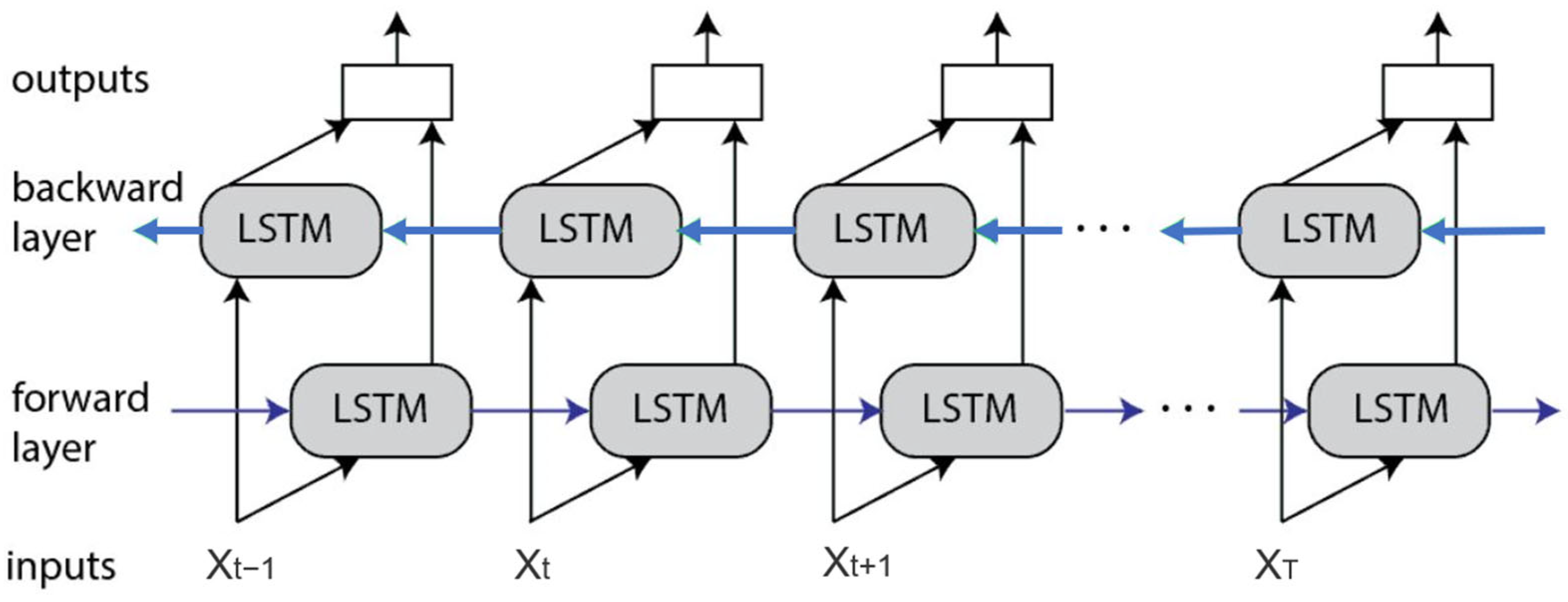
From the above neural networks, we know that the training process of BP neural networks, RNNs, or LSTM always predicts the output of the next moment from front to back based on the temporal information of the previous moment. Such a training method cannot maximize the hidden intrinsic information in the time series of ship trajectory data and does not make good use of the data. In contrast, the bidirectional long short-term memory (BiLSTM) neural network model used in this paper is good at mining data with long-term dependencies in long time series, and it has a more powerful representation and learning ability.

The network structure of BILSTM is the same as the standard LSTM neural network structure, which also consists of basic cell states, input gates, forgetting gates, and output gates. The basic principle of the BILSTM neural network is composed of a forward LSTM and a standard backward LSTM, and the structure of the BILSTM neural network is shown in Figure 4:

The BILSTM neural network introduced in this paper has the output of $\overrightarrow{{\mathrm{h}}_{\mathrm{t}}}$ from two opposite directions, i.e., the output of the forward network is $\overleftarrow{{\mathrm{h}}_{\mathrm{t}}}$ and the output of the backward network is $\overleftarrow{{\mathrm{h}}_{\mathrm{t}}}$. The expressions for the computation of the forward and backward outputs are

$$\overrightarrow{{\mathrm{h}}_{\mathrm{t}}}=\overrightarrow{\mathrm{L}\mathrm{S}\mathrm{T}\mathrm{M}}\left({\mathrm{x}}_{\mathrm{t}},\overrightarrow{{\mathrm{h}}_{\mathrm{t}-1}}\right)$$

(18)

$$\overleftarrow{{\mathrm{h}}_{\mathrm{t}}}=\overleftarrow{\mathrm{L}\mathrm{S}\mathrm{T}\mathrm{M}}\left({\mathrm{x}}_{\mathrm{t}},\overleftarrow{{\mathrm{h}}_{\mathrm{t}-1}}\right)$$

(19)

The output is the combined output of the forward and backward results stacked into

$${\mathrm{H}}_{\mathrm{t}}=\overrightarrow{{\mathrm{h}}_{\mathrm{t}}}+\overleftarrow{{\mathrm{h}}_{\mathrm{t}}}$$

(20)

2.3. Pre-Processing of Data

The AIS data selected for the experiments in this paper were collected on 2 August 2020, and the ship with MMSI number 636017973 was selected from the Huangze Yang sea area, with a total of 2753 ship track points. AIS data processing first involved data cleaning and pre-processing to ensure the quality and relevance of the data. Key features were then extracted from the data, including the vessel speed, heading, and trajectory characteristics such as dwell time, as well as vessel behavior patterns in specific environments, such as obstacle avoidance and steering. These features were then used to train a ship trajectory prediction model using deep learning techniques. The goal of the model is to accurately predict a ship’s position in the short term to improve the safety and efficiency of maritime navigation.

2.3.1. Trajectory Data Cleaning

• Cleaning trajectory points with too-small a time interval

In order to reduce the redundancy of the input data features, the ship trajectory data points with small time intervals need to be eliminated. Set two adjacent points of the ship navigation trajectory as P_i and P_(i+1); when the time interval between these two points is less than a certain threshold, then this part of data should be deleted, and when the time threshold between the two points is greater than a certain threshold, then these data should be kept.

2.

Cleaning the trajectory data of abnormal speed and heading

In this paper, the set sailing speed is 30 knots. In order to achieve the purpose of improving the prediction accuracy, ship trajectory data with a sailing speed of greater than 30 knots are deleted, and the range of the amplitude of the heading is set between 0 and 360; sailing data with headings not in the range of 0 to 360 are deleted.

2.3.2. Interpolation Processing of Trajectory Data

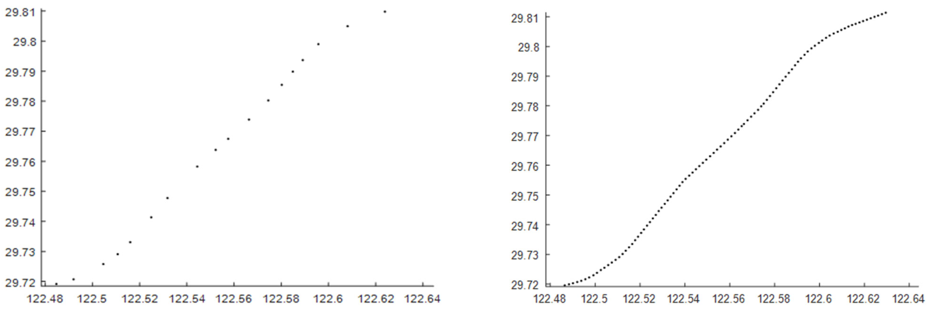
In this paper, a section of the trajectory of the vessel with MMSI No. 636017973 sailing at sea on 2 August 2020 was obtained via ShipHub. Since the observation moments are sparse and not uniform enough, the time intervals of the data features input to the model are unequal, so the model has difficulty in extracting the navigation characteristics of the target ship from these unevenly spaced navigation data. For this kind of non-uniform time-series data with unequal time intervals, the common processing method is to use an interpolation algorithm to fit the historical trajectory data and then to sample uniformly to predict the sailing trajectory based on the obtained trajectory data with equal time intervals.

The interpolation method used in this paper is the constant directional Mercator algorithm, which is used to calculate the range D and heading C of two waypoints $\left({\mathrm{l}\mathrm{a}\mathrm{t}}_1,{\mathrm{l}\mathrm{o}\mathrm{n}}_1\right)$, $\left({\mathrm{l}\mathrm{a}\mathrm{t}}_2,{\mathrm{l}\mathrm{o}\mathrm{n}}_2\right)$ at the same time so that the average speed v between the two points can be obtained; the waypoint $\left({\mathrm{l}\mathrm{a}\mathrm{t}}_1,{\mathrm{l}\mathrm{o}\mathrm{n}}_1\right)$ is used as the starting point, and the waypoint is carried out with speed v to obtain the waypoint of the same time interval, whereby the range D and heading C are calculated as follows:

$$\mathrm{C}=\arctan \left(\frac{\left|\mathrm{D}\mathsf{\lambda }\right|}{\left|\mathrm{D}\mathrm{M}\mathrm{P}\right|}\right)=\arctan \left(\frac{|{\mathrm{l}\mathrm{a}\mathrm{t}}_1-{\mathrm{l}\mathrm{a}\mathrm{t}}_2|}{|{\mathrm{M}\mathrm{P}}_2-{\mathrm{M}\mathrm{P}}_1|}\right)$$

(21)

$$\mathrm{D}=\mathrm{D}\mathsf{\phi }\sec \mathrm{C}=\left({\mathrm{l}\mathrm{o}\mathrm{n}}_1-{\mathrm{l}\mathrm{o}\mathrm{n}}_2\right)\ast \sec \mathrm{C}$$

(22)

The interpolation of the track points in this paper is performed with a time interval of 30 s as a way of obtaining the ship trajectory with a uniform time distribution. The plots of some of the track segments before and after the interpolation of the target-ship track points are shown in Figure 5:

2.3.3. Partitioning of the Trajectory Data Set

This study selected historical trajectory data from over 3200 vessels in the Zhoushan sea area, sourced from the Navigation Project research team at Ningbo University, as the foundation for model training. To ensure data representativeness, this study analyzed AIS data from a randomly selected day each month between March and September 2022. these vessel trajectory data consist of continuous sequences of positional points, meticulously recording key navigation information such as longitude, latitude, heading, and speed. Within this dataset, each unique vessel identifier corresponds to a specific vessel trajectory, while certain vessel identifiers are associated with multiple trajectories. Through analysis of the initial segments of each trajectory, the model trained during the training phase can capture both general navigation patterns and specific behaviors, such as changes in speed and turning maneuvers. This enables the trained model to accurately predict the future positions of vessels, particularly at critical turning points, based on previously learned patterns when receiving new trajectory data.

After cleaning the original trajectory data and interpolating the data, the training, validation, and test sets of trajectory data need to be divided. Firstly, the historical ship trajectory data are divided into samples, i.e., data samples corresponding to the input form of the prediction model. The sliding window length set in this paper is 12, i.e., the observed time, latitude and longitude, speed, and heading of the first 12 moments are set as known information, and the position information of the 13th moment is set as unknown information, and all sample data are generated according to this rule. The first 70% of all sample data are divided into the training data set, 10% of the articulated data are divided into the validation data set, and the last 20% are divided into the test data set. This completes the pre-processing of the ship trajectory data.

2.3.4. Prediction Model Evaluation Metrics

This study selects the root mean square error (RMSE) as the evaluation metric to assess the quality of the model’s predictive performance.

The error between the prediction point P′ and the observation point P at the i-th moment in the model can be expressed as

$${\mathrm{e}}_{\mathsf{\lambda }}={\mathsf{\lambda }}_{\mathrm{i}}^{\prime }-{\mathsf{\lambda }}_{\mathrm{i}}$$

(23)

$${\mathrm{e}}_{\mathsf{\phi }}={\mathsf{\phi }}_{\mathrm{i}}^{\prime }-{\mathsf{\phi }}_{\mathrm{i}}$$

(24)

In this context, ${\mathrm{e}}_{\mathsf{\lambda }}$ and ${\mathrm{e}}_{\mathsf{\phi }}$ represent the longitude and latitude errors, respectively, between the predicted point P′ and the observed point P at the i-th time instance. Here, ${\mathsf{\lambda }}_{\mathrm{i}}^{\prime }$ and ${\mathsf{\phi }}_{\mathrm{i}}^{\prime }$ denote the predicted longitude and latitude values, while ${\mathsf{\lambda }}_{\mathrm{i}}$ and ${\mathsf{\phi }}_{\mathrm{i}}$ stand for the actual longitude and latitude values. In this paper, in order to be able to evaluate the prediction results of the model more intuitively, the surface arc distance between the observation point and the prediction point is used as the evaluation criterion, in which the surface arc distance ${\mathrm{d}\mathrm{i}\mathrm{s}\mathrm{t}}_{\mathrm{i}}$ between the observation point and the prediction point is calculated as follows:

$${\mathrm{S}}_{\mathrm{i}}=\sin \left({\mathsf{\lambda }}_{\mathrm{i}}^{\prime }\right)\ast \sin \left({\mathsf{\lambda }}_{\mathrm{i}}\right)\ast \cos \left({\mathsf{\phi }}_{\mathrm{i}}^{\prime }-{\mathsf{\phi }}_{\mathrm{i}}\right)+\cos \left({\mathsf{\lambda }}_{\mathrm{i}}^{\prime }\right)\ast \mathrm{c}\mathrm{o}\mathrm{s}\left({\mathsf{\lambda }}_{\mathrm{i}}\right)$$

(25)

$${\mathrm{d}\mathrm{i}\mathrm{s}\mathrm{t}}_{\mathrm{i}}=\mathrm{R}\ast \arccos \left({\mathrm{S}}_{\mathrm{i}}\right)\ast \mathsf{\pi }/180$$

(26)

where $\mathrm{R}$ denotes the mean radius of the earth and takes the value of 6371.004 km.

The formula for calculating the root mean square error is shown below:

$${\mathrm{R}\mathrm{M}\mathrm{S}\mathrm{E}}_{\mathsf{\lambda }}=\sqrt{\frac{1}{\mathrm{n}}\sum _{\mathrm{i}=1}^{\mathrm{n}}{\left({\mathsf{\lambda }}_{\mathrm{i}}^{\prime }-{\mathsf{\lambda }}_{\mathrm{i}}\right)}^2}$$

(27)

$${\mathrm{R}\mathrm{M}\mathrm{S}\mathrm{E}}_{\mathsf{\phi }}=\sqrt{\frac{1}{\mathrm{n}}\sum _{\mathrm{i}=1}^{\mathrm{n}}{\left({\mathsf{\phi }}_{\mathrm{i}}^{\prime }-{\mathsf{\phi }}_{\mathrm{i}}\right)}^2}$$

(28)

$${\mathrm{R}\mathrm{M}\mathrm{S}\mathrm{E}}_{\mathrm{d}\mathrm{i}\mathrm{s}\mathrm{t}}=\sqrt{\frac{1}{\mathrm{n}}\sum _{\mathrm{i}=1}^{\mathrm{n}}{\left({\mathrm{d}\mathrm{i}\mathrm{s}\mathrm{t}}_{\mathrm{i}}\right)}^2}$$

(29)

In the above equation, ${\mathrm{R}\mathrm{M}\mathrm{S}\mathrm{E}}_{\mathsf{\lambda }},$ ${\mathrm{R}\mathrm{M}\mathrm{S}\mathrm{E}}_{\mathsf{\phi }}$ and ${\mathrm{R}\mathrm{M}\mathrm{S}\mathrm{E}}_{\mathrm{d}\mathrm{i}\mathrm{s}\mathrm{t}}$ represent the root mean square error in the longitude, latitude, and distance directions, respectively; n represents the number of test samples; $({\mathsf{\lambda }}_{\mathrm{i}},{\mathsf{\phi }}_{\mathrm{i}})$ represents the true value of the i-th sample; $({\mathsf{\lambda }}_{\mathrm{i}}^{\prime },{\mathsf{\phi }}_{\mathrm{i}}^{\prime })$ represents the predicted value of the i-th sample, and ${\mathrm{d}\mathrm{i}\mathrm{s}\mathrm{t}}_{\mathrm{i}}$ represents the error of the distance between the predicted value and the true value of the surface arc of the i-th sample.

The formula for calculating the accuracy is as follows:

$${\mathrm{M}\mathrm{A}\mathrm{P}\mathrm{E}}_{\mathsf{\lambda }}=\frac{100\mathrm{\%}}{n}{\sum }_{i=1}^n\left|\frac{{\mathsf{\lambda }}_{\mathrm{i}}-{\mathsf{\lambda }}_{\mathrm{i}}^{\prime }}{{\mathsf{\lambda }}_{\mathrm{i}}}\right|$$

(30)

$${\mathrm{M}\mathrm{A}\mathrm{P}\mathrm{E}}_{\mathsf{\phi }}=\frac{100\mathrm{\%}}{n}{\sum }_{i=1}^n\left|\frac{{\mathsf{\phi }}_{\mathrm{i}}-{\mathsf{\phi }}_{\mathrm{i}}^{\prime }}{{\mathsf{\phi }}_{\mathrm{i}}}\right|$$

(31)

MAPE is primarily utilized to quantify the proportion of deviation between model-predicted values and actual values. By computing the average, it offers an intuitive percentage indicator regarding the prediction accuracy. Lower MAPE values signify a higher prediction accuracy, making it particularly suitable for assessing the average error level of prediction results.

2.4. Setting of Parameters

Once the model has been built and trained, Optuna performs a Bayesian optimization based on the sample information to find the set of hyperparameters that are likely to result in the highest accuracy of trajectory prediction. This is followed by a nearby search. One of the main features it applies to the model is trial and error, budgeting the possible final results based on the learning curve and eliminating them early if the prediction is bad. Its efficiency is shown more clearly when the model is complex and training is slow due to a large amount of data.

In the designed experiments, Optuna ran for a total duration of 3 h, 16 min and 16 s, exploring 30 combinations of hyperparameters. During the optimization process in Optuna, the Objective Value represents the objective function value for each trial, while the Best Value signifies the best objective function value found so far. The Objective Value is evaluated based on the mean absolute percentage error (MAPE) in the validation set, calculated as the model’s loss value for each trial on the validation set. The Best Value corresponds to the minimum MAPE achieved on the validation set during the optimization process, indicating the optimal model performance obtained thus far. Despite the relatively small number of combinations attempted, the subsequent results exhibited an accuracy exceeding 98%, with the initial few returns demonstrating an accuracy of 93%. The process of parameter tuning, along with the optimization history, is illustrated in Figure 6. The optimal model structure is shown in

Table 1. Optimal model structure.

Number of Hidden Layers	1
BILSTM layer: number of nodes, dropouts, activation function	350, 0.25, ReLU
Output layer: number of nodes, activation function	2, sigmoid
Batch size	32
Epochs	250
Learning Rate	0.27
Loss	0.002271022451067804
Optimizer	adam

:

Here are the definitions of the relevant parameters to be optimized in the model:

Activation function: Activation functions introduce non-linearity to neural networks. Common choices include ReLU, Sigmoid, and Tanh.

Batch size: The number of training samples used in each iteration to update the model parameters.

Epochs: The number of complete passes of the entire training dataset through the neural network during training.

Optimizer: Algorithms that adjust the neural network parameters to minimize the loss function. Common optimizers include Adam, RMSprop, and SGD.

Learning rate: Governs the size of parameter updates during optimization. Affects the convergence speed and model performance.

3. Visual Analysis of Trajectory Prediction

According to the above experimental method, the AIS data LOG, LAT, SOG, and COG of the experimental vessel are used as input samples of the Optuna–BILSTM network model. The position LON and LAT of the experimental vessel are used as the output samples of the model, and the experimental results are shown in Figure 7.

The models subjected to experimental comparison in this study encompass the Optuna–BILSTM model, the BILSTM model, the LSTM model, and the BP model proposed herein. These models were empirically fine-tuned manually, with the exception of the Optuna–BILSTM model, which underwent automatic tuning. The efficacy of the Optuna–BILSTM model was verified through the analysis of vessel trajectories derived from AIS data, evaluating, and contrasting its accuracy metrics (RMSE, MAPE, R2, and p) against those of the BP, LSTM, BILSTM, and other models. The comparative outcomes, presented in Table 1, demonstrate that the Optuna–BILSTM model consistently exhibits the lowest prediction error across six ships; it achieved an average MAPE value of 0.0043, surpassing the BP, LSTM, and BILSTM models, which recorded values of 0.031, 0.011, and 0.069, respectively. Similarly, the RMSE value for the Optuna–BILSTM model stood at 0.0044, notably lower than that of the BP (0.020), LSTM (0.096), and BILSTM (0.044) models. Moreover, the Optuna–BILSTM model attained the highest R2 score of 0.9972 compared with the BP (0.8628), LSTM (0.9413), and BILSTM (0.9649) models. Consequently, the Optuna–BILSTM model demonstrated superior performance across all evaluated metrics.

As shown in

Table 2. Prediction errors of trajectories of four ships with different models.

MMSI	Evaluation Indicators	BP	LSTM	BILSTM	Optuna–BILSTM
413380410	MAPE	0.035	0.016	0.0056	0.0087
	RMSE	0.026	0.0112	0.0068	0.0089
	R2	0.8566	0.9132	0.9893	0.9979
413456950	MAPE	0.034	0.0089	0.0091	0.0028
	RMSE	0.023	0.0091	0.0098	0.0024
	R2	0.8465	0.9347	0.9413	0.9997
413457220	MAPE	0.023	0.0053	0.0043	0.0026
	RMSE	0.012	0.0054	0.0041	0.0030
	R2	0.8756	0.9884	0.9945	0.9969
414400930	MAPE	0.033	0.012	0.0089	0.0032
	RMSE	0.018	0.0129	0.0091	0.0033
	R2	0.8726	0.9291	0.9347	0.9946
Average value	MAPE	0.031	0.011	0.0069	0.0043
	RMSE	0.020	0.0096	0.0074	0.0044
	R2	0.8628	0.9413	0.9649	0.9972
p-value	MAPE	0.006	0.189	0.131	-
	RMSE	0.006	0.028	0.066	-

, p-values were utilized to ascertain the statistical significance of performance disparities between the Optuna–BILSTM model and comparative models. Specifically, p-values of 0.06 for both MAPE and RMSE in relation to the BP model underscore the superior performance of the Optuna–BILSTM model. Likewise, a p-value of 0.028 for RMSE when compared with the LSTM model further confirms the Optuna–BILSTM’s enhanced predictive accuracy for this metric. In contrast, p-values exceeding 0.05 for the BILSTM model indicate no significant performance difference with the Optuna–BILSTM model, though R2 results suggest the latter’s consistent superiority. Notably, for vessels 413380410, 413457220, and 414400930, R² values for the Optuna–BILSTM model were 0.8%, 0.2%, and 6% higher, respectively, compared with the BILSTM model. The almost identical predicted and observed trajectories for vessel 413456950, with an R2 value of 0.9997 from the Optuna–BILSTM model, further attest to its predictive precision. Overall, the Optuna–BILSTM model demonstrates enhanced performance over the BP, LSTM, and BILSTM models in ship trajectory prediction, as visually summarized in the metric comparison in Figure 8.

Figure 8 demonstrates that the Optuna–BILSTM model outshines others in this study, showcasing superior performance across both curved and straight trajectories. The BP model, a multilayer feedforward neural network trained via the error backpropagation algorithm, stands as one of the most utilized neural network models. However, its applicability to time-series data prediction is limited, resulting in suboptimal predictions with an average R2 value. In contrast, LSTM and BILSTM models, designed specifically for time-series data, address issues of gradient explosion or vanishing that may occur with the accumulation of previous data in the RNN input process. Consequently, the LSTM model surpasses the BP model in predictive outcomes, and the BILSTM model, augmenting the LSTM with a reverse time-series data-extraction layer, excels by extracting more data features, thereby enhancing the prediction performance. The selection of parameters within these prediction models is pivotal, yet achieving optimal parameters through personal expertise or manual experimentation is challenging and time-consuming. On average, the Optuna–BILSTM model predicts 7% better than other models; therefore, the Optuna–BILSTM model is identified as the most suitable model for prediction. Predicting the course of a ship is an important issue in ensuring navigational safety. Currently, numerous prediction methodologies leverage diverse models, including LSTM, RNN, and GRU, to forecast outcomes. To enhance the precision of the prediction model, this research employs Optuna for the optimal configuration of the BILSTM model’s parameters. Subsequently, a deep learning model is trained on four distinct trajectories. The Optuna framework’s efficient parameter search capability markedly boosts the model’s computational efficiency by swiftly pinpointing the optimal network parameters and structure. This optimization significantly diminishes the duration needed for model training and prediction. Secondly, from testing on multiple datasets, the model shows good generalization ability, which means that it not only performs well on the training set, but is also able to adapt and accurately predict unseen data, demonstrating its strong adaptability in dealing with the problem of predicting ship trajectories in different sea areas and weather conditions. In addition, the Optuna–BILSTM model also demonstrates excellent anti-noise capability, which can effectively deal with noise and outliers in the AIS data, ensuring the stability and reliability of the prediction results. In conclusion, the model excels not only in its prediction accuracy, but also in its efficient computational performance, powerful generalization capability, and excellent anti-noise properties, making it a powerful tool in the field of maritime ship trajectory prediction.

4. Conclusions

In this study, we have proposed a model that combines Optuna and BILSTM for predicting ship trajectories. The model is designed to overcome the limitations of traditional BP neural networks in dealing with long-time-series problems and to perform hyperparameter optimization using Optuna. The aim is to improve the accuracy and performance of trajectory prediction. In this study, trajectory data from four vessels were used as a benchmark to evaluate the model’s performance. By comparing with traditional BP neural network, LSTM and BILSTM models, this study validates the superiority of the proposed Optuna–BILSTM model. The results show that the model exhibits higher accuracy and robustness in the ship trajectory prediction task. The hyperparameter optimization of Optuna enables an automatic search for the best model hyperparameter configuration, which further improves the model performance. This combined approach allows for a better adaptation of the model structure and parameter settings to specific ship trajectory prediction tasks. In addition, this study reveals another advantage of the proposed model, namely its ability to extract important features. By learning patterns and trends in the trajectory data, the model is able to capture the key features that influence the ship’s trajectory. This ability can be used to reduce the error in predicting the ship’s tracking point by using the extracted features. Consistent with the aims of scholar Vladimir Brozovic’s research, which emphasizes the enhancement of maritime safety and the prevention of ship collisions at sea, the Optuna–BILSTM trajectory prediction model holds significant promise [34]. With its ability to effectively predict vessel trajectories based on historical data, the model can play a pivotal role in mitigating the risk of collisions and ensuring safer maritime navigation.

Ultimately, this research has practical applications for maritime traffic controllers. By accurately predicting ship trajectories, ships can take the necessary precautions in advance to avoid collisions. This not only helps to improve the efficiency of maritime traffic but also enhances maritime safety.

References

- Rødseth, Ø.J.; Perera, L.P.; Mo, B. Big Data in Shipping—Challenges and Opportunities. In Proceedings of the 15th International Conference on Computer Applications and Information Technology in the Maritime Industries (COMPIT 2016), Lecce, Italy, 9–11 May 2016. [Google Scholar]
- Jing, C.; Changwei, Y.; Shi, D.; Jian, F.; Hujun, W. A novel spatiotemporal multigraph convolutional network for air pollution prediction. Appl. Intell. Int. J. Artif. Intell. Neural Netw. Complex Probl. -Solving Technol. 2023, 53, 18319–18332. [Google Scholar]
- Feng, H.; Cao, G.; Xu, H.; Ge, S.S. IS-STGCNN: An Improved Social spatial-temporal graph convolutional neural network for ship trajectory prediction. Ocean. Eng. 2022, 266, 112960. [Google Scholar] [CrossRef]
- Passenier, P.O. An adaptive track predictor for ships. Electr. Eng. Math. Comput. Sci. 1987, 2, 14. [Google Scholar]
- Tang, X.M.; Chen, P.; Li, B. Optimal air route flight conflict resolution based on receding horizon control. Aerosp. Sci. Technol. 2016, 50, 77–87. [Google Scholar] [CrossRef]
- Last, P.; Bahlke, C.; Hering-Bertram, M.; Linsen, L. Comprehensive Analysis of Automatic Identification System (AIS) Data in Regard to Vessel Movement Prediction. J. Navig. 2014, 67, 791–809. [Google Scholar] [CrossRef]
- Johansen, T.A.; Cristofaro, A.; Perez, T. Ship Collision Avoidance Using Scenario-Based Model Predictive Control. IFAC Conf. Control. Appl. Mar. Syst. 2017, 49, 4–21. [Google Scholar]
- Xiao, J.L.; Li, X.L. Vessel traffic flow prediction method based on ensemble empirical mode decomposition and back propagation neural network optimized with differential evolution algorithm. Dalian Haishi Daxue Xuebao/J. Dalian Marit. Univ. 2018, 44, 9–14. [Google Scholar]
- Schller, C.; Aravantinos, V.; Lay, F.; Knoll, A. What the Constant Velocity Model Can Teach Us About Pedestrian Motion Prediction. Cornell Univ. 2019, 5, 1696–1703. [Google Scholar] [CrossRef]
- Jiang, B.; Guan, J.; Zhou, W.; Chen, X. Vessel Trajectory Prediction Algorithm Based on Polynomial Fitting Kalman Filtering. J. Signal Process. 2019, 5, 741–746. [Google Scholar]
- Rong, H. TAPS Ship trajectory uncertainty prediction based on a Gaussian Processmodel. Ocean Eng. 2019, 182, 499–511. [Google Scholar] [CrossRef]
- Murray, B.; Perera, L.P. A Data-Driven Approach to Vessel Trajectory Prediction for Safe Autonomous Ship Operations. In Proceedings of the 13th International Conference on Digital Information Management (ICDIM 2018), Berlin, Germany, 24–26 September 2018. [Google Scholar]
- Agarwal, S. Data Mining: Data Mining Concepts and Techniques. In Proceedings of the 2013 International Conference on Machine Intelligence and Research Advancement, Katra, India, 21–23 December 2013. [Google Scholar]
- Jiang, D.; Wu, B.; Van Gelder, P.H.A.J. Towards a probabilistic model for estimation of grounding accidents in fluctuating backwater zone of the Three Gorges Reservoir. Life Cycle Reliab. Saf. Eng. 2020, 205, 107239. [Google Scholar] [CrossRef]
- Tran, Q.; Firl, J. Online maneuver recognition and multimodal trajectory prediction for intersection assistance using non-parametric regression. In Proceedings of the 2014 IEEE Intelligent Vehicles Symposium Proceedings, Dearborn, MI, USA, 8–11 June 2014. [Google Scholar]
- Lin, Y.; Zhang, J.W.; Liu, H. An algorithm for trajectory prediction of flight plan based on relative motion between positions. Front. Inform. Tech. Electron. Eng. 2018, 19, 905–916. [Google Scholar] [CrossRef]
- Wu, K.; Pan, W. A four-dimensional flight trajectory prediction model based on data mining. Comput. Appl. 2007, 11, 2637–2639. [Google Scholar]
- Tang, H. YYSH A model for vessel trajectory prediction based on long short-term memory neural network. J. Mar. Eng. Technol. Proc. Inst. Mar. Eng. Sci. Technol. 2022, 21, 136–145. [Google Scholar]
- Li, G. Track Prediction for HF Radar Vessels Submerged in Strong Clutter Based on MSCNN Fusion with GRU-AM and AR Model. Remote Sens 2021, 13, 2164. [Google Scholar]
- Zhong, C. JZCX Inland ship trajectory restoration by recurrent neural network. J. Navig. 2019, 72, 1359–1377. [Google Scholar] [CrossRef]
- Vries, G.K.D.D.; Someren, M.V. Machine learning for vessel trajectories using compression, alignments and domain knowledge. Expert Syst. Appl. 2012, 39, 13426–13439. [Google Scholar] [CrossRef]
- Zissis, D. XEKL Real-time vessel behavior prediction. Evol. Syst.-Ger. 2016, 7, 29–40. [Google Scholar] [CrossRef]
- Xu, T.; Liu, X.; Yang, X. Ship Trajectory Online Prediction Based on BP Neural Network Algorithm. In Proceedings of the 2011 International Conference of Information Technology, Computer Engineering and Management Sciences, Nanjing, China, 24–25 September 2011. [Google Scholar]
- Zhou, H.; Chen, Y.; Zhang, S. Ship Trajectory Prediction Based on BP Neural Network. J. Artif. Intell. 2019, 1, 29. [Google Scholar] [CrossRef]
- Rumelhart, D.E.; Hinton, G.E.; Williams, R.J. Learning Representations by Back Propagating Errors. Nature 1986, 323, 533–536. [Google Scholar] [CrossRef]
- Vennerød, C.B.; Kjærran, A.; Bugge, E.S. Long short-term memory RNN. arXiv 2021, arXiv:2105.06756. [Google Scholar]
- Cho, K.; van Merrienboer, B.; Gulcehre, C.; Bahdanau, D.; Bougares, F.; Schwenk, H.; Bengio, Y. Learning phrase representations using RNN encoder-decoder for statistical machine translation. arXiv 2014, arXiv:1406.1078. [Google Scholar]
- Shi, Z.; Xu, M.; Pan, Q.; Yan, B.; Zhang, H. LSTM-based Flight Trajectory Prediction. In Proceedings of the 2018 International Joint Conference on Neural Networks (IJCNN), Rio de Janeiro, Brazil, 8–13 July 2018. [Google Scholar]
- Graves, A.; Schmidhuber, J. Framewise phoneme classification with bidirectional LSTM and other neural network architectures. Neural Netw. 2005, 18, 602–610. [Google Scholar] [CrossRef] [PubMed]
- Siami-Namini, S.; Tavakoli, N.; Namin, A.S. The Performance of LSTM and BiLSTM in Forecasting Time Series. In Proceedings of the 2019 IEEE International Conference on Big Data (Big Data), Los Angeles, CA, USA, 9–12 December 2019. [Google Scholar]
- Liu, S.; Ma, D.; Meng, X. Ship track prediction based on CNN and Bi-LSTM. J. Chongqing Univ. Technol. (Nat. Sci.) 2020, 3, 196–205. [Google Scholar]
- Bergstra, J.; Bengio, Y. Random Search for Hyper-Parameter Optimization. J. Mach. Learn Res. 2012, 13, 281–305. [Google Scholar]
- Akiba, T.; Sano, S.; Yanase, T.; Ohta, T.; Koyama, M. Optuna: A Next-generation Hyperparameter Optimization Framework. In Proceedings of the 25th ACM SIGKDD International Conference on Knowledge Discovery & Data Mining, Anchorage, AK, USA, 4–8 August 2019; pp. 2623–2631. [Google Scholar] [CrossRef]
- Brozovic, V.; Kezic, D.; Bosnjak, R.; Krile, S. Implementation of International Regulations for Preventing Collisions at Sea Using Coloured Petri Nets. J. Mar. Sci. Eng. 2023, 11, 1322. [Google Scholar] [CrossRef]
Figure 1.
Network composition of a BP neural network.
Figure 2.
The unfolding structure of an RNN.
Figure 3.
LSTM neural network structure diagram.
Figure 4.
Structure of the BiLSTM neural network.
Figure 5.
Comparison of track points before and after interpolation processing of the trajectory data.
Figure 6.
Diagram of the parameter optimization process.
Figure 7.
Longitude and latitude predictions for ship 413380410.
Figure 8.
Trajectory prediction chart for four vessels.