1. Introduction
A hemodynamic model is able to provide theoretical evidence for suitable selections of clinical treatment plan, and hence has important meanings. Take human physiology as an example: if the heart is regarded as a power source and the arteries at each level as transportation pipelines, the human microcirculation system can be seen as the system load. There is a complex coupling relationship between various components of the circulation system, which influence each other severely. A change in one factor can even cause a change in the environment of the entire circulation system. Complex phenomena in the human blood circulation system should be the properties produced by the coupling of various parts of the system, not only relying on the selection of boundary conditions. Therefore, a well-developed hemodynamic model must be able to show completely different components of the circulation system and their effects. Only in this way can it provide a correct simulation of the numerous phenomena of human blood flow, and provide evidence for research on producing and developing principles for dealing with some diseases.
Nowadays, there are many studies on the hemodynamics model, but none of them is able to show the properties of the human circulation system. Though the hemodynamic model of a rigid tube wall [
1,
2,
3,
4] has been widely utilized, it is not able to show the stress-strain properties of solids, which places severe limitations on clinical applications. The model of a flexible tube wall [
5,
6,
7] is not only able to show the deformation of the solid, but also reflects the influence of solid deformation on flow field, which has great potential for application [
8]. However, the model fails to show the complex pressure wave of physiology [
9] and simulate the propagation of a pulse wave. In these studies, the outlet pressures were all set as a fixed value or a measured value, and it was assumed that these outlet conditions will not change with the change of the flow field. Since pressure influences the deformation of the tube wall, the change of outlet pressure conditions will have a profound influence on the flow field. Therefore, the results were not ideal in those studies relating to the adjustment process of the entire human circulation system [
10]. In the study on myocardial bridge [
11], Schwarz observed the influence of changes of downstream flow field on the front-end flow field. It follows that changeable load condition is one of the most important components neglected in most hemodynamic models. Through analysis of the characteristics of a capillary microcirculation system and the flow properties of the kidney and other organs, it was found that the seepage in porous media is a load model that accords relatively well with the form of physiological changes. Therefore, this paper needs to add a load of porous media seepage in the classical bi-directional liquid-solid coupling model to completely simulate the human circulation system.
Additionally, in order to make the load of porous media seepage accord with physiology, there are requirements for the tube length and other flow field factors. The human microcirculation system is located at the end of the human blood circulation system. Before arriving at the microcirculation system, the fluid will flow through the entire circulation system and experience severe changes. However in previous studies, the flow field was not long enough for the simulation of these changes, so the model requires a flow field that is equivalent to the actual physiology to simulate the physiological flow field correctly. In addition, the deformation of tube wall is an important factor influencing the flow field. Thus, in the calculating simulation of Dong [
12], as the influence of liquid-solid coupling was not considered, his simulation results were not very satisfying, though the load of porous media seepage was also selected. It can be seen that a bi-directional liquid-solid coupling model with enough developing space for a flow field is the precondition for a load to produce correct results. Only when all the factors in this system can meet physiological needs can the results accord with physiology.
Accordingly, this paper built a bi-directional liquid-solid model with long straight tube to simulate the human blood vessel. A load of porous media seepage was arranged at the outlet of the liquid-solid coupling model to simulate the human microcirculation system. Using the most ideal single-pulse inlet condition and free outlet’s boundary condition, we successfully simulated various complex phenomena in human blood vessels. The mechanisms of these phenomena were revealed through analysis. Moreover, the heart rate was changed for a comparison with human physiological reality, thus verifying the reliability of the model proposed.
2. Model and Methods
2.1. Hemodynamic Model
According to the discussions above, this paper built a model of a long straight tube with a flexible wall and a load of porous media seepage. As shown in
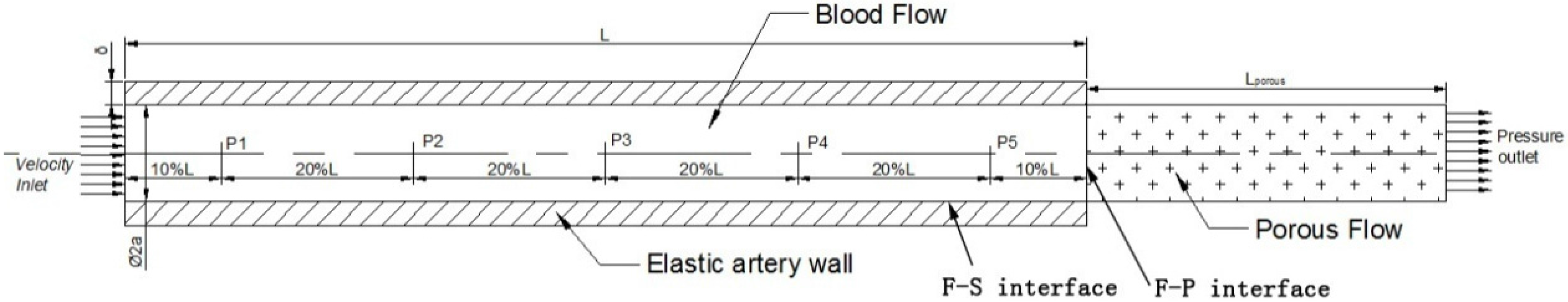
Figure 1, the model mainly consists of three parts: the straight tube is used for simulating the flow field region of the blood vessel; the flexible tube wall is used for simulating deformation of the vascular wall and its influence on flow; and the tube with porous media seepage is used for simulating flow in the microcirculation system. The control equations of the various regions are as follows:
2.1.1. Fluid Region
Momentum equation:
where
is fluid velocity,
p is fluid pressure,
is fluid density, and
is the fluid stress tensor. The configuration of the fluid region is changeable.
2.1.2. Solid Region
Structural momentum equation:
Solid constitutive equation:
where
is the solid stress tensor,
is the Lagrange elasticity tensor, and
is the strain tensor.
2.1.3. Liquid-Solid Coupling Interface:
where
is the stress tensor, n is the normal vector, and u is the velocity vector of the interface.
2.1.4. Region with Porous Media Seepage
Momentum equation:
where
k is permeability,
is porosity, and
is the fluid viscosity factor.
2.1.5. Fluid-Porous Media Seepage Interface
where
is the momentum exchange capacity of the interface;
is the interface conductivity, which is determined by the constitutive equation of porous media seepage;
V is velocity.
Figure 1.
Calculation model and schematic of measuring point distribution.
Figure 1.
Calculation model and schematic of measuring point distribution.
2.2. Simulate Method
In order to comprehensively show the properties of the model, this paper selected the entire blood circulation system starting from the aorta as a study subject. The whole aorta has a straight tube of about 1 m. Because of the scale and strain rate of the aorta, the fluid was simplified as the Newtonian fluid [
13]. The straight tube was set with a length of 1000 mm, diameter of 20 mm, and wall thickness of 2 mm, which accords with the aortal physiological parameters. The tube with porous media for seepage had a length of 300 mm, ensuring its internal flow developing completely. As the power source of the blood circulation system, the inlet took velocity as its boundary condition. Outlet was set as free outlet, located at the end of the tube with porous media for seepage.
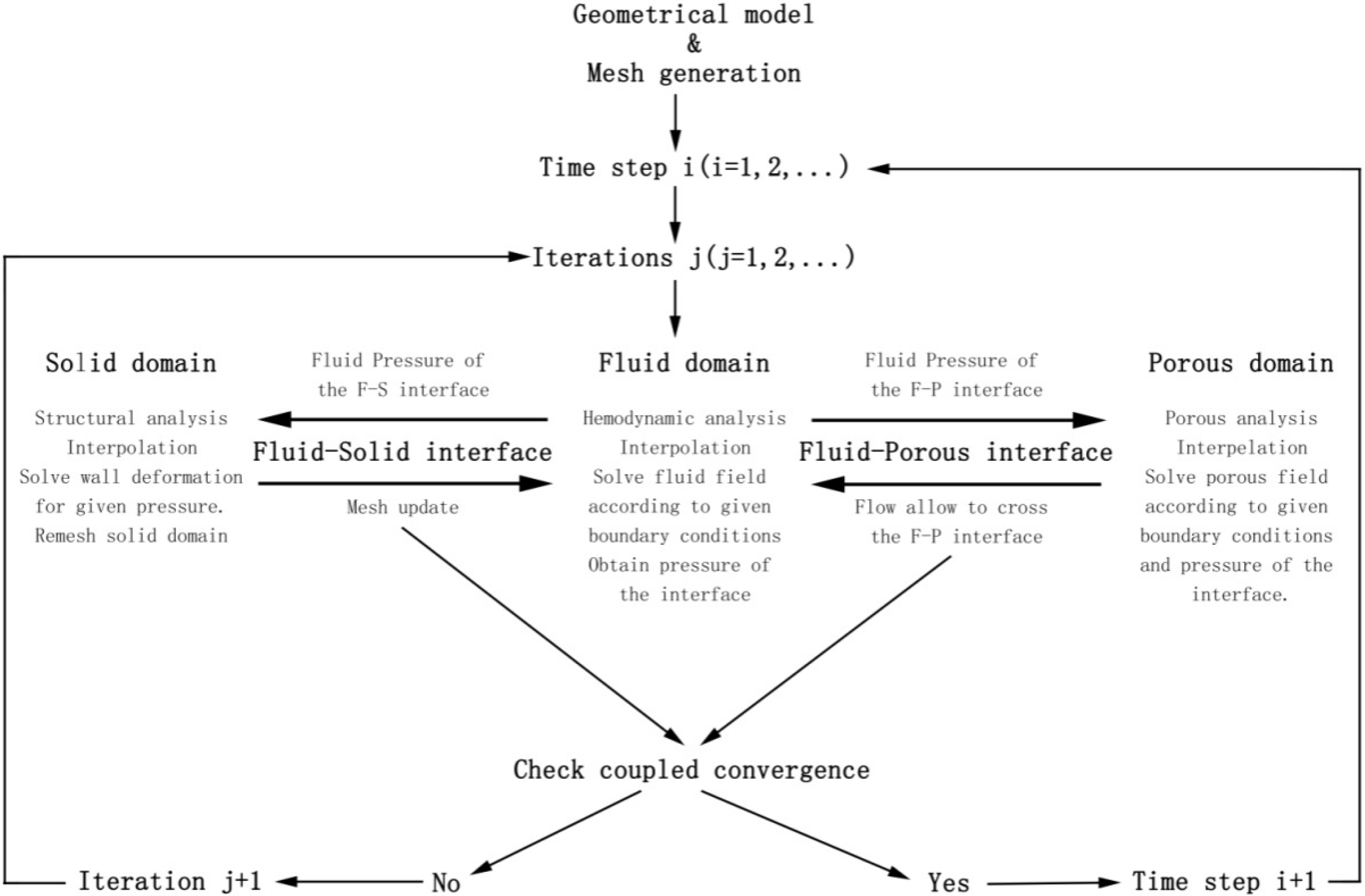
The Computational methodology process of the hemodynamic model is shown in
Figure 2. On the liquid-solid interface, fluid applied the calculated wall pressure on the solid; after the solid was deformed due to the pressure, the flow field grid was rebuilt. Then, after several iterations, a convergent result was obtained. Notably, due to the change in the flow field region, the fluid would be temporarily stored in the deformation; when the pressure in the tube dropped, the deformation would decrease and those stored fluids would reenter the flow field to flow. On the fluid-porous media seepage interface, fluid provided the pressure on interface. Under this pressure, the total fluid amount allowed to go through the seepage tube could be calculated. In this system, though solid and porous media seepage did not interact directly on an interface, they were connected together by the flow field. Therefore, the three parts operate synergistically, creating a complex multi-directional coupling relationship.
Figure 2.
Computational methodology.
Figure 2.
Computational methodology.
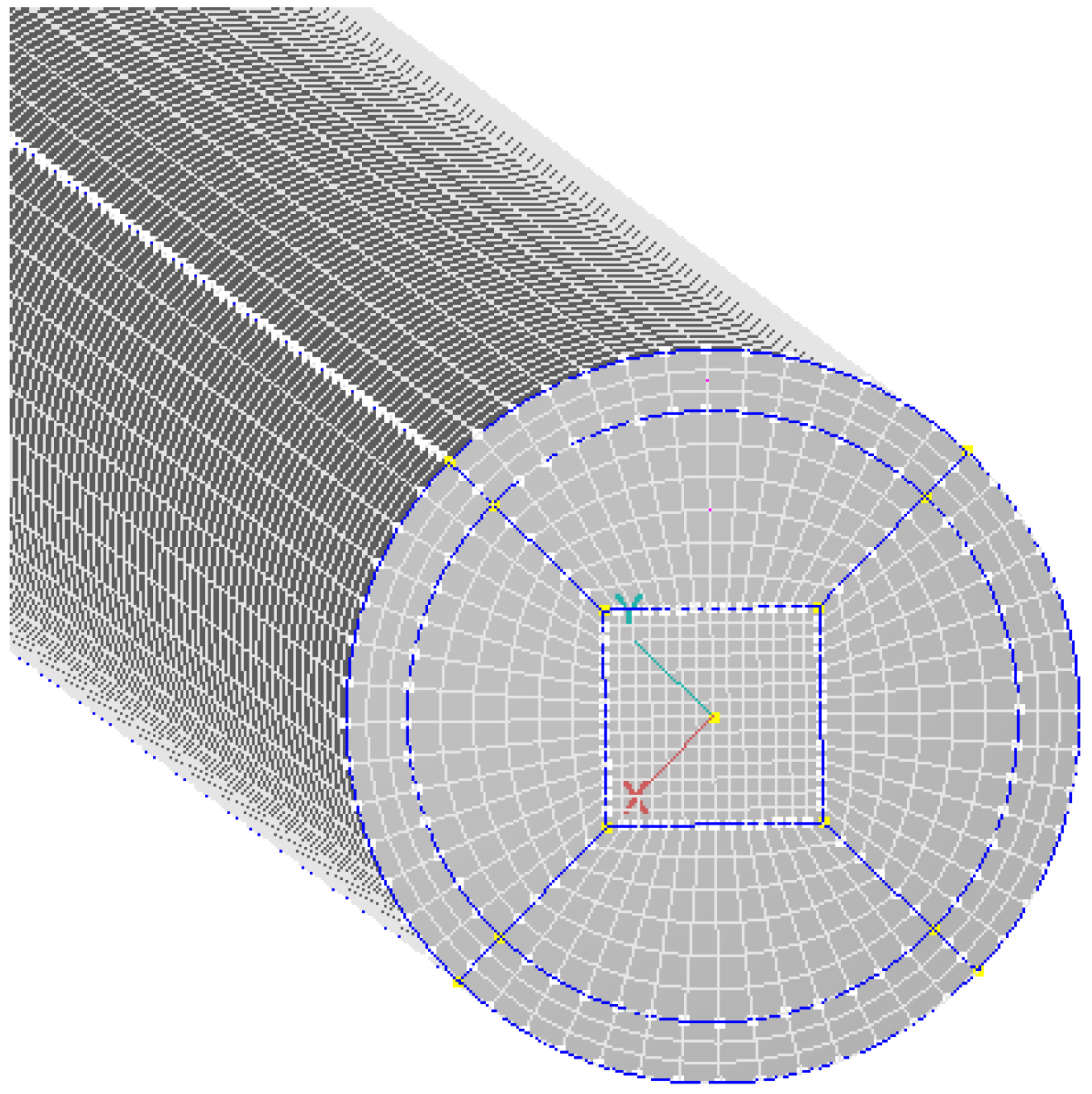
This paper divided the model into a structural grid. As shown in
Figure 3, the tube cross-section was divided into butterfly grids. The model finally consisted of 84,728 cells, with 107,850 nodes. Therein, the fluid region had 52,668 cells, the solid region had 16,632 cells, and the tube with porous media for seepage had 15,428 cells. CFD-ACE SOLVER was chosen to carry out the entire calculation for this paper, and an arbitrary Lagrangian-Eulerian (ALE) method was employed. The first-order upwind difference scheme was used. A constant time step Δ
t = 0.02 s was employed in this study. When the program was running, corresponding physical quantities such as pressure and displacement transfer across fluid-structure interfaces through the coupling of the two sets of codes until a convergence criterion (10
−4) was reached for each time step. Repeated computations with a finer grid (253,800 nodes, 205,386 cells) and coarser grid (33,165 nodes, 24,220 cells) were carried out. Results showed that the alteration of maximum pressure at the same location of the fluid domain was 6% between the finer grid and the coarser grid, and alteration was 3% between the finer grid and the grid in this paper.
Figure 3.
Grid division for the tube cross-section.
Figure 3.
Grid division for the tube cross-section.
2.3. Calculation Examples and Parameters
In order to verify the reliability and superiority of the hemodynamic model proposed, five calculation examples (see
Table 1) were taken through changing the tube length, load conditions, and cardiac cycle. All the calculation examples were based on the physiological parameters of the descending aorta, and the transient flow was adopted for simulating actual the working state of a blood vessel. The fluid in the tube was simplified as the Newtonian fluid of blood parameters, with a density of 1050 kg/m
3 and a dynamic viscosity coefficient of 0.0035 Pa·s [
14]. The density of the flexible tube wall was 1120 kg/m
3, Young’s modulus was 0.5 MPa [
15], and Poisson’s ratio is 0.49 [
16]. The permeability of the porous media was
, and the porosity was 100%.
Table 1.
Five calculation examples and their parameters.
Table 1.
Five calculation examples and their parameters.
| Calculation Examples | Permeability of Porous Media k | Length of Flow Field | Cardiac Cycle T |
|---|
| Example 1. Normal physiology | | 1000 mm | 0.8 |
| Example 2. No seepage load | N/A | 1000 mm | 0.8 |
| Example 3. Short tube | | 200 mm | 0.8 |
| Example 4. Accelerated heart rate | | 1000 mm | 0.6 |
| Example 5. Decreased heart rate | | 1000 mm | 1 |
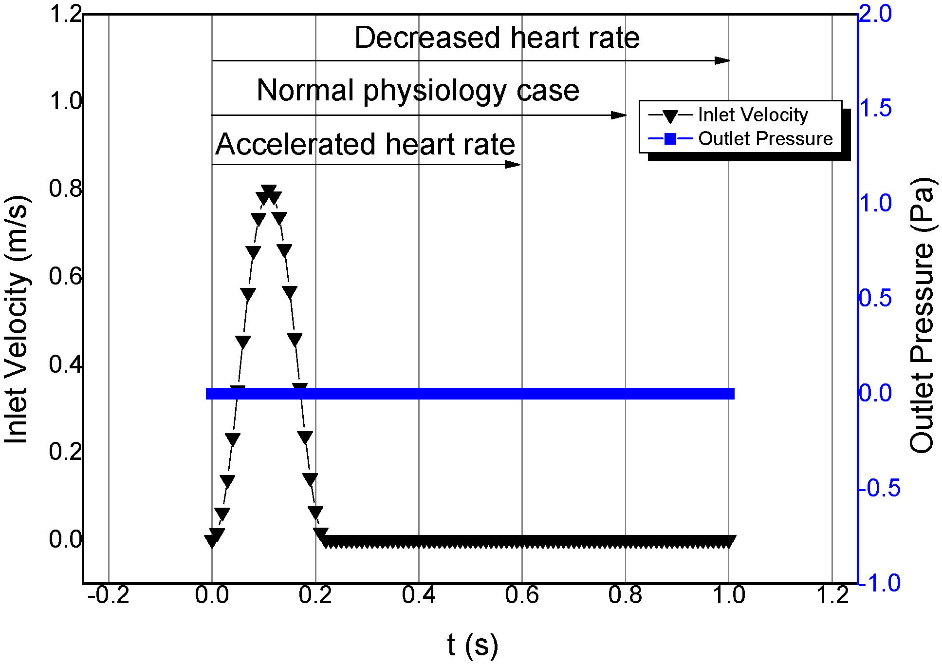
All the calculation examples selected velocity inlet condition and free outlet, and the inlet condition and outlet condition are shown in
Figure 4. The inlet condition was velocity inlet, which was used for simulating the process of cardiac impulse. Systole was 0–0.2 s, and the maximum systolic velocity was 0.8 m/s [
17]. Diastole ranged from 0.2 s to the end of a cardiac cycle. Inlet velocity at this period was kept at 0 m/s to simulate the state of a closed heart valve without reflux. The average Reynolds number was about 661, which was based on the average velocity of the inlet. The flow regime was laminar flow. The outlet condition was pressure-free,
i.e., the pressure was always kept at 0 Pa. This not only eliminated the influence of disturbance from outer pressure factors, but also achieved similarity with the physiological reality in the vein.
For the two calculation examples where the heart rate was changed, this paper assumed the outflow after every heart pulse to be consistent. Thus one only has to change the length of the diastole to achieve a change in the cardiac cycle. As shown in
Figure 4, for different cardiac cycle calculation examples, the systole was kept unchanged while the diastole changed. Accordingly, in the example of normal physiology, heart rate was 75/min and cardiac cycle was 0.8 s (0.2 s for systole, and 0.6 s for diastole); in the example of accelerated heart rate, heart rate was 100 min
−1 and cardiac cycle was 0.6 s (0.2 s for systole, and 0.4 s for diastole); in the example of decreased heart rate, heart rate was 60 min
−1 and cardiac cycle was 1 s (0.2 s for systole, and 0.8 s for diastole).
Figure 4.
Boundary condition of the flow field.
Figure 4.
Boundary condition of the flow field.
3. Results and Discussion
This paper firstly compared the calculation example with no seepage load. Using the index of vascular pressure, the rationality of the liquid-solid coupling hemodynamic model with seepage load proposed in this paper was analyzed. Then, through simulation of pressure wave propagation, reflection, and other physiological phenomena in the blood vessel, the importance of the length of the straight tube was analyzed, which supports the reliability of the model proposed. Finally, the superiority of the model was discussed from the formation of secondary pressure wave in blood vessel and the influence of cardiac cycle.
In the process of data analysis, in order to show the different variation forms in the entire flow field at different positions, this paper selected five measuring points in the tube. All of them were located in the center of the tube cross-section. As shown in
Figure 1, the distances of the five measuring points P1–P5 from the inlet were 0.1 m, 0.3 m, 0.5 m, 0.7 m, and 0.9 m, respectively. Under such a configuration, we could comprehensively master the similarities and differences at each position of the tube, through analysis of the pressure-time relationship at various measuring points of the flow field. In addition, we could analyze phase differences of various feature points in one cycle.
3.1. Physiological Pressure Level
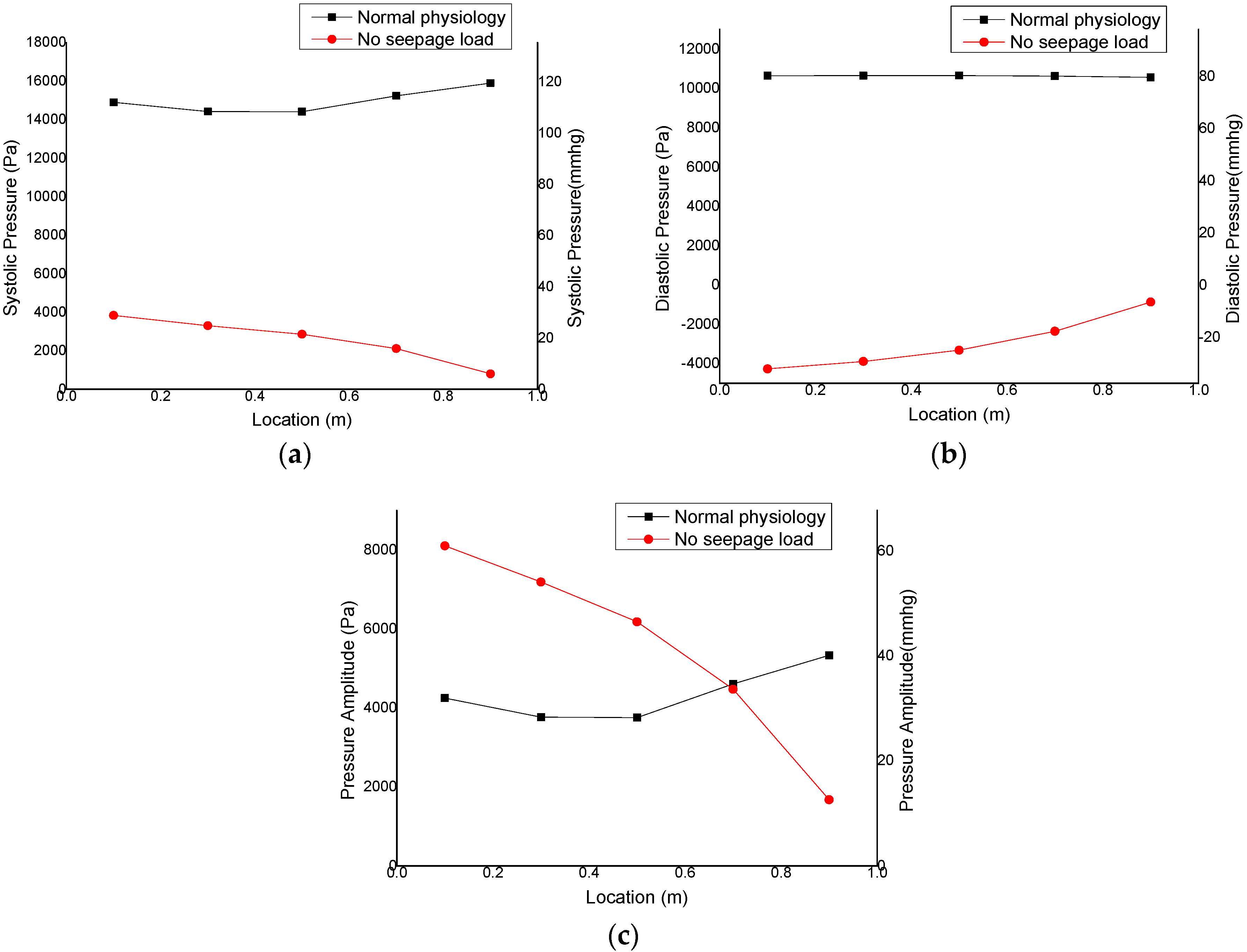
Calculation results showed that the influence of load on the flow field was tremendous. Thus, between calculation examples with load and without load, the properties of flow field exhibited major differences. In
Figure 5, there is a comparison between the pressure results of calculation examples with normal physiology and no seepage load. Therein, A is the systolic pressure of various positions in the tube, B is the diastolic pressure, and C is the amplitude of the pressure in the tube. In the example of normal physiology, the systolic pressure of all positions in the tube was maintained at around 120 mmHg; the diastolic pressure was kept at 80 mmHg, and the amplitude of pressure at 30–40 mmHg. These observations accorded with the physiological reality. In the example without seepage load, the systolic pressure near the inlet was 29 mmHg, while that near the outlet was 6 mmHg. The diastolic pressure near the inlet was −32 mmHg, while that near the outlet was −6 mmHg. With the approach to the outlet, the amplitude decreased continuously. It can be seen that the use of pressure alone as the outlet condition led to a larger negative pressure, and the pressure amplitude in the tube was changing. These results do not accord with the physiological conditions. The seepage load played a role in impeding flow in the model, which had a great effect on whether the fluid would be stored in the deformation of the tube wall. Thus the pressure in the tube was redistributed and reached the physiological pressure level.
Figure 5.
Comparisons of pressure in the examples with seepage load and pressure-free outlet: (a) maximum vascular pressure; (b) minimum vascular pressure; (c) pressure amplitude.
Figure 5.
Comparisons of pressure in the examples with seepage load and pressure-free outlet: (a) maximum vascular pressure; (b) minimum vascular pressure; (c) pressure amplitude.
Through studying the process of the flow field developing in the tube, the internal mechanism of how the normal physiology example maintained the physiological pressure level can be revealed. When the load had a very strong hindering effect, the fluid entering the flow field was not able to flow out completely. Part of the fluid was stored in the deformation of tube wall and participated in the next cardiac cycle. Thus, the initial pressure of the second cycle would be increased. After several cardiac cycles, when the initial pressure of the flow field increased to a certain level, the newly input fluid was able to pass through the load and flow out of the flow field in one cycle. Accordingly, the fluid in the tube resumed a stable state, and the initial pressure of flow field also reached a dynamic balance.
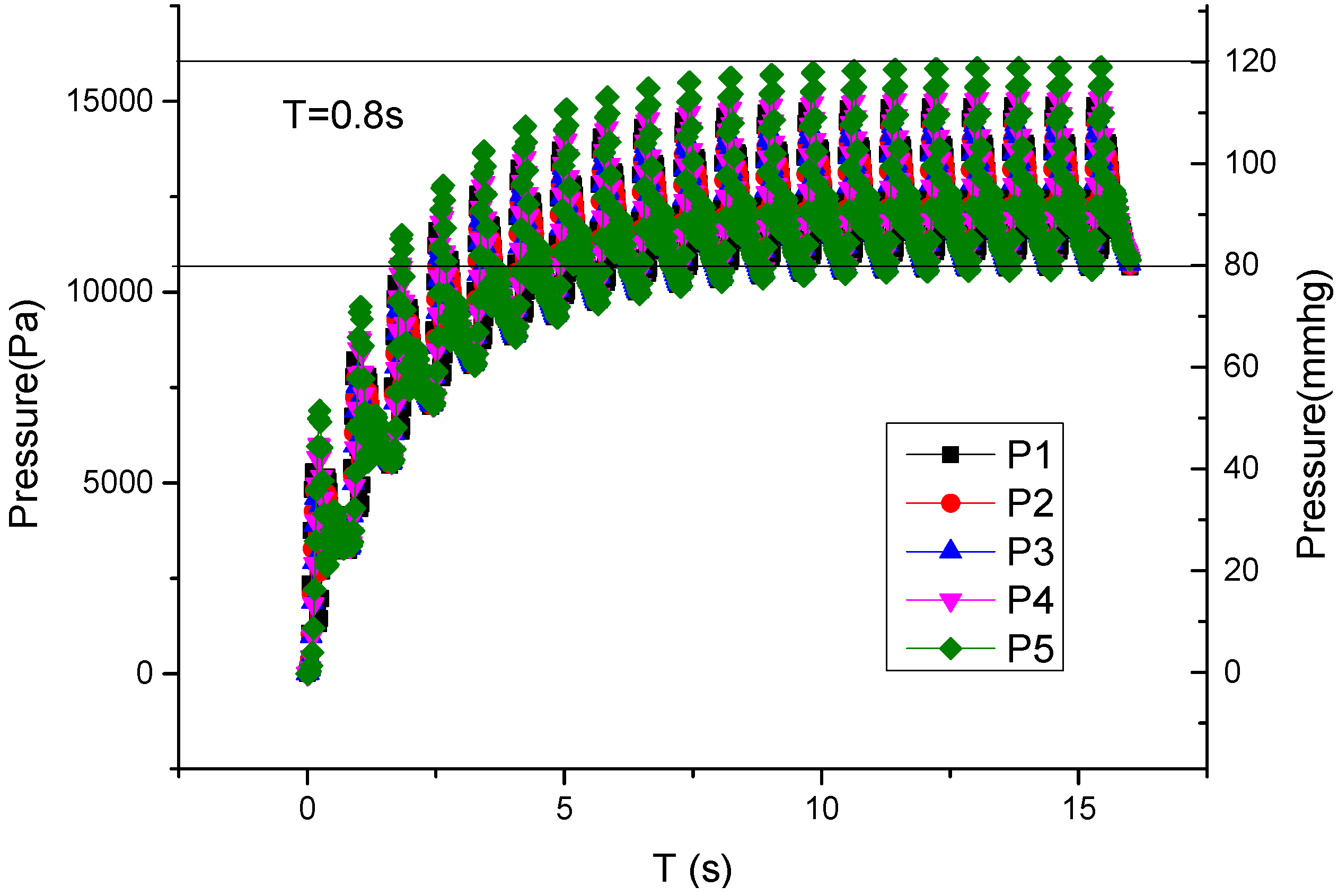
Figure 6 is the curve of pressure change with time in the flow field of the normal physiology example, which shows the whole process of flow field developing from completely static to stable. The five lines in the figure represent the five positions from inlet to outlet in the tube. The time ranged from 0 s to 16 s, with 20 cycles in total. It can be seen from the figure that the pressure in flow field increased rapidly from 0 s to 7 s, and gradually became stable after 7 s. The final pressure at all measuring points in the tube was kept in the range of physiological pressure of 80–120 mmHg. This indicates that the load influenced the total fluid quantity stored through the elastic deformation of tube wall, which further influenced the systolic pressure, diastolic pressure, and pressure amplitude in the tube.
Figure 6.
Changing process of pressure in the tube from static flow field (P1–P5 are five measuring points distributing axially along the tube).
Figure 6.
Changing process of pressure in the tube from static flow field (P1–P5 are five measuring points distributing axially along the tube).
3.2. Pulse Wave Propagation
This model showed very complex phenomena in time and in space, which included the propagation of pulse wave. When fluid entered the tube, fluid would be stored in the increased flow field from tube wall deformation, which would not cause influence for downstream flow field temporarily. Due to such property, the moments when the pressure wave peak occurred at various positions of the tube were different.
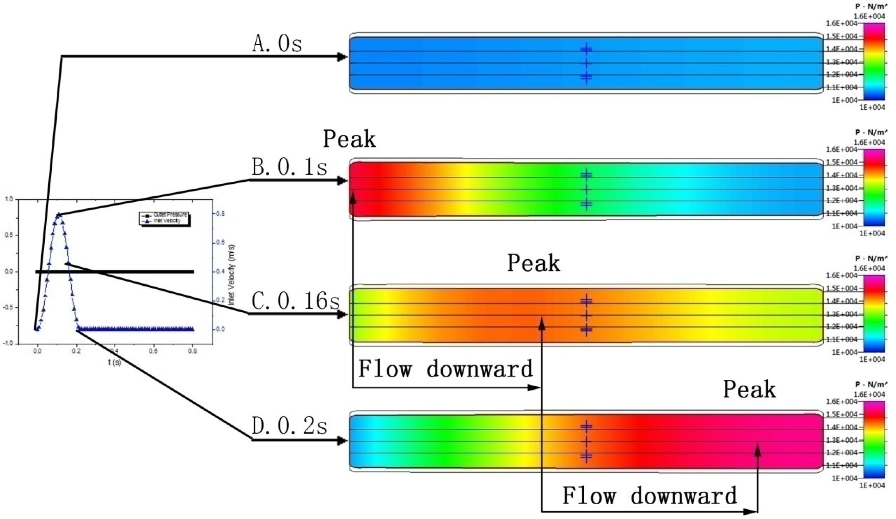
Figure 7 is the pressure nephogram of the tube cross-section, wherein A, B, C, and D represent four moments (0 s, 0.1 s, 0.16 s, and 0.2 s, respectively). From the nephogram, we can clearly observe the propagation of the pressure wave peak, that is, the propagation of the pulse wave. At the initial moment, the pressure in the tube was maintained at a stable value. At 0.1 s, inlet velocity just reached the wave peak, and the inlet pressure reached the maximum. At 0.16 s, the pressure wave peak started to move forward, and the pressure decreased on both sides of the wave peak. Until0.2 s, the pressure wave peak was near the outlet. Comparing the flow field of these moments, the whole process of the pressure wave peak moving from inlet to outlet can be seen distinctly. This is the same as the result of Olson’s research [
18]. According to the academic monograph of Fung [
13], propagation of the pulse wave exists widely. Therefore, it is necessary to take the effect of the pulse wave into account in hemodynamic simulations.
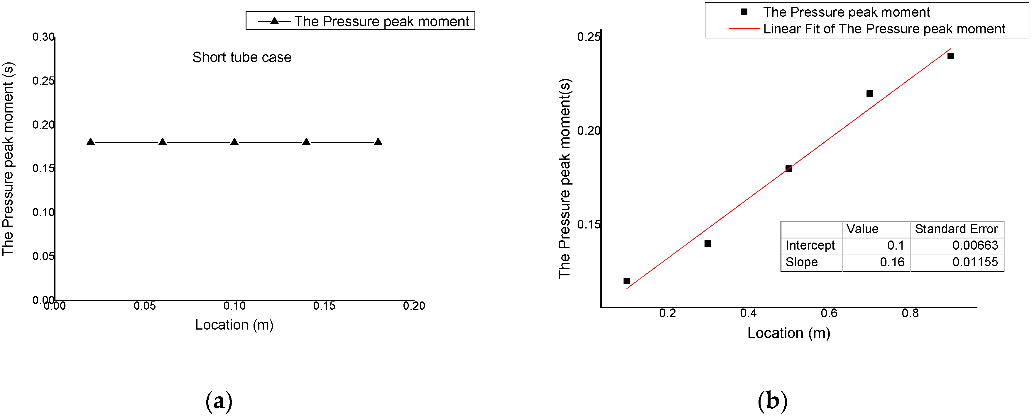
Results of the short tube example show that the difference in peak occurring moment was small. As shown in
Figure 8a, the pressure peak values in tube all occurred at 0.18 s. The tube with a length of only 200 mm failed to show the phenomenon of pressure wave propagation. Comparatively, in the model of this paper, the tube length was the same as the actual aorta length. This provided the flow field with enough developing space. It follows that tube length is one of the essential conditions for simulation results to accord with the physiological reality.
Through data treatment, the moments when pressure peaks occurred at five measuring points were obtained and subjected to linear fitting, as seen in
Figure 8b. It can be seen that the measuring point P1 at 0.1 m away from the inlet reached the pressure maximum first. Other measuring points showed the pressure peak value successively; the closer to the inlet, the earlier the peak occurred. The two measuring points at 0.1 m and 0.9 m away from the inlet had a time difference of 0.12 s in the occurrence of pressure peak. Through the linear fitting for peak-occurring moments, we can obtain the relationship between peak-occurring moment and the distance from inlet. According to the fitting result, the velocity of the pulse wave in the tube was 6.25 m/s, which is close to the actual pulse wave velocity [
19]. Also, it is the same as the one-dimensional pressure wave velocity [
20]. This confirms that this model was able to correctly simulate the pulse wave propagation in human aortas.
Figure 7.
Pressure nephograms (A. t = 0 s; B. t = 0.1 s; C. t = 0.16 s; D. t = 0.2 s).
Figure 7.
Pressure nephograms (A. t = 0 s; B. t = 0.1 s; C. t = 0.16 s; D. t = 0.2 s).
Figure 8.
Moments corresponding to the pressure peak and their fitting results: (a) peak-occurring moments in short tube example; (b) peak-occurring moments in a normal physiology example.
Figure 8.
Moments corresponding to the pressure peak and their fitting results: (a) peak-occurring moments in short tube example; (b) peak-occurring moments in a normal physiology example.
3.3. Pulse Wave Reflection
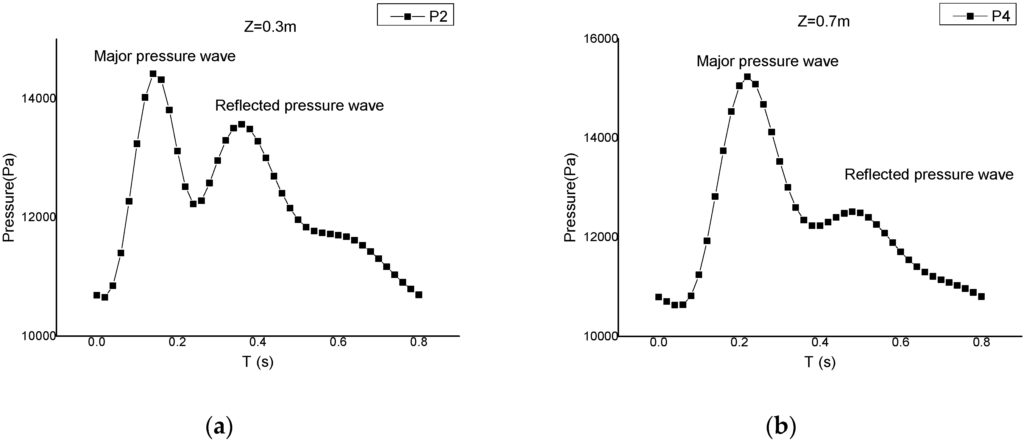
Another phenomenon shown in the model is the reflection of the pulse wave. When pressure propagated to the load interface, seepage load played a hindering effect. Accordingly, not all the fluid was able to flow out of the flow field smoothly; part of it would be held in the flow field. At this time the tube wall near the outlet would expand, and the pressure would increase accordingly. When the pressure downstream was larger than that upstream, it would also propagate back towards the inlet, producing a reflection wave. If the pulse wave is taken as a major pressure wave, this reflection wave is typically called a secondary pressure wave. By overlapping this reflection wave with the incoming major pressure wave, a pressure-time curve with double wave peaks can be produced. In previous studies, such a curve failed to be simulated. However, in the results of physiological measurement and of simulation by our model, such a curve shape with a double wave peak was visible.
Figure 9 shows a pressure-time curve, plotted with the observations of two measuring points at 0.3 m and 0.7 m away from the inlet. We can clearly see the double peak structure from the figure. The pressure-time curve was formed through the overlapping of a major pressure wave and a reflection wave; the reflection wave was obviously smaller than the major pressure wave. Comparing the curves of the two measuring points, it can be seen that though the difference between major pressure waves was not large, there was a significant difference between reflection waves.
Figure 9.
Pressure-time curves of measuring points: (a) P2 (0.3 m); (b) P4 (0.7 m).
Figure 9.
Pressure-time curves of measuring points: (a) P2 (0.3 m); (b) P4 (0.7 m).
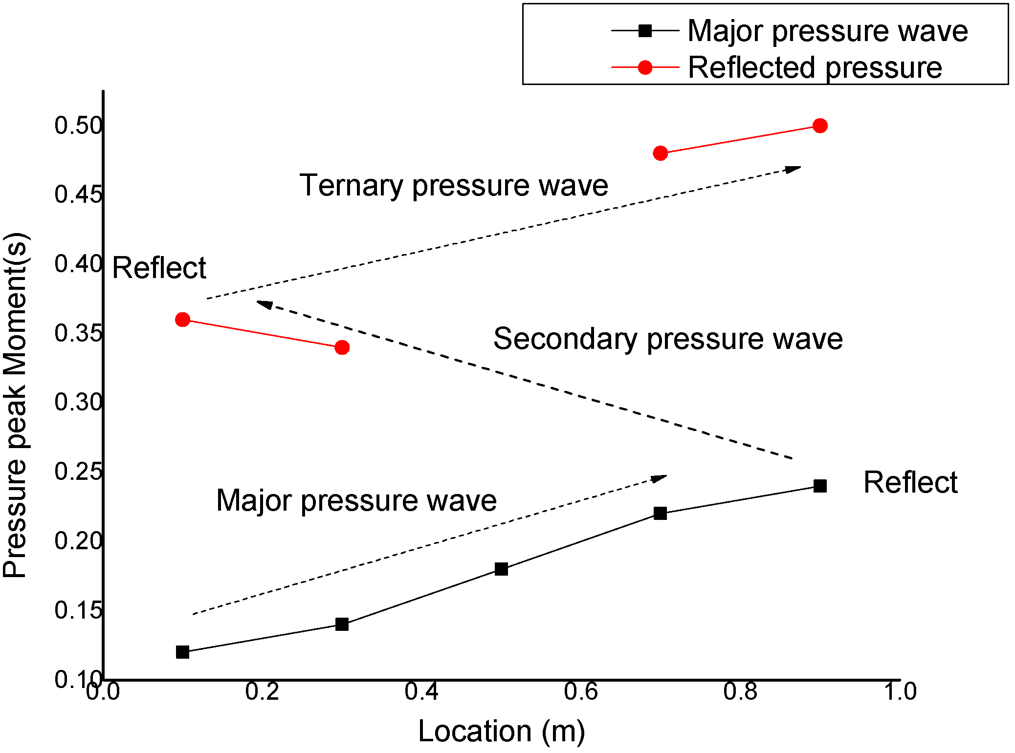
This paper studied the occurring moments of the major pressure wave peak and reflection wave peak, as shown in
Figure 10. It can be seen that the occurring moments of major pressure peak were in linear relationship with distance. However, the reflection wave peak presented a non-linear feature, e.g., the peak-occurring time was earlier at the position of 0.3 m than at the position of 0.1 m, while it was earlier at the position of 0.7 m than at the position of 0.9 m. This exactly suggests that secondary pressure wave is also propagated in the form of a wave. As shown by marks of the figure, the major pressure wave was a non-reflected primary pressure wave, propagating towards the outlet. However, at the positions of 0.3 m and 0.1 m, the pressure waves were secondary pressure waves that have been reflected once by the load and hence propagated towards the inlet. Similarly, the pressure waves at 0.7 m and 0.9 m were the third pressure waves that experienced another reflection by the inlet, and propagated towards the outlet again. Conclusively, in
Figure 9, the reflection wave at 0.3 m was the secondary pressure wave undergoing one reflection, and that at 0.7 m was the third pressure wave undergoing two reflections. That is why there was a large difference between the magnitudes of reflection waves at these two positions.
Through comparing with physiological measurements [
9], it can be seen that the secondary pressure wave simulated by the model of this paper accords with the physiological reality. Without the coupling of liquid-solid-porous media seepage, it is impossible to simulate this physiological blood pressure, which is produced by repeated reflections and overlapping of pressure waves. In addition, this complex wave shape produced a profound influence on the flow field by influencing the tube wall deformation. The wall shear stress and other flow field parameters would change accordingly. Therefore, the simulation of this paper accords with the physiological reality, and this complex wave structure is also an important guarantee for the correctness of the study later.
Figure 10.
Moments corresponding to major pressure peak and reflection wave peak.
Figure 10.
Moments corresponding to major pressure peak and reflection wave peak.
3.4. Influence of Cardiac Cycle
In order to verify the reliability of the model in terms of physiological parameter change, this paper used the cardiac cycle as the study subject. In human physiological phenomena, a change in the cardiac cycle has a great influence on the pressure in a blood vessel. The blood flux output after every cardiac pulse is fixed. However, with a change in the cardiac cycle, the time of fluid flowing out of the flow field will change, and the pressure required by a fluid to pass through the load will increase, finally influencing the pressure in the tube. Therefore, the pressure change caused by heart rate is not only related to flux but also has a close connection with vascular wall deformation and load. It can be seen that the influence of the cardiac cycle on vascular pressure is produced by a coupling of multiple factors, and all factors in the system are required to accord with the physiological reality. In a numerical simulation, a short straight tube could not meet the needs of storing fluid, and normal pressure outlet conditions could not change with the tube's flow field. Hence, both could not simulate the pressure change caused by cardiac cycle change. Comparatively, the model in this paper provides fluid with enough developing space and storing ability, as well as the load condition changing with the flow field. Therefore it can complete the task the numerical simulation cannot. This paper selected two cardiac cycles (0.6 s and 1 s), and compared them with the normal physiology example.
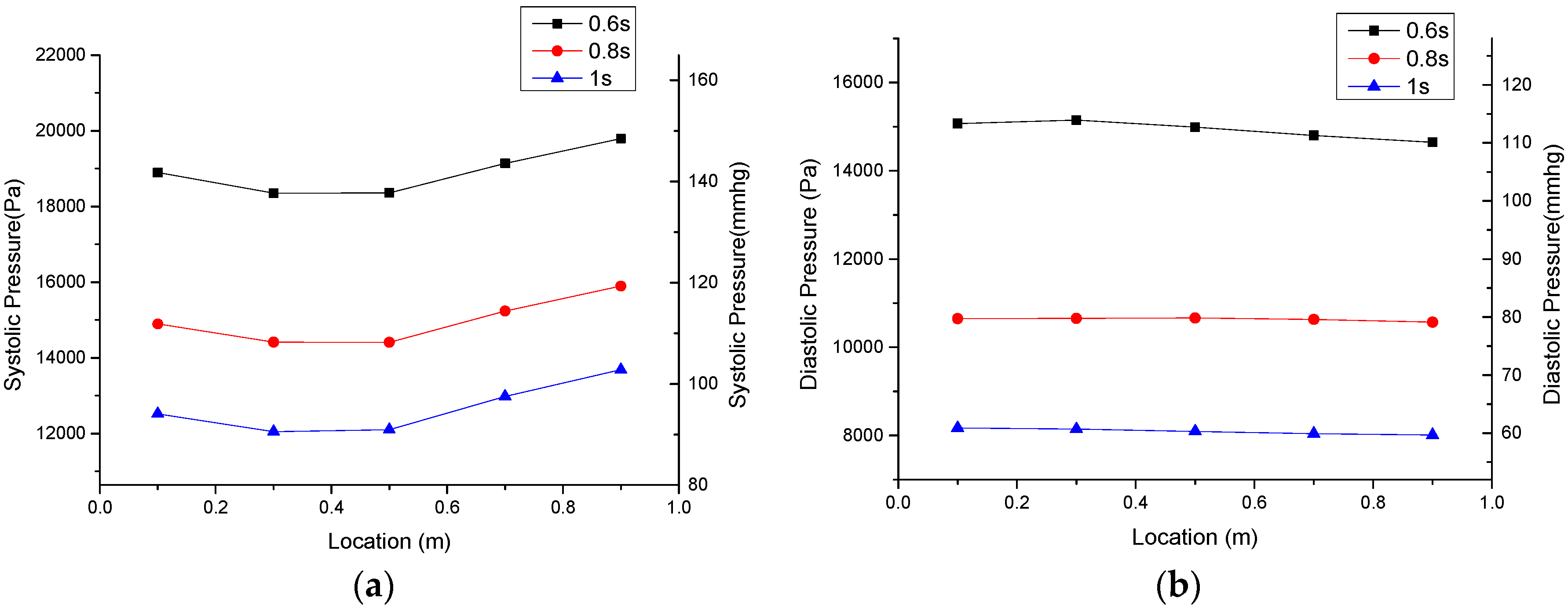
First, this paper analyzed the systolic pressure and diastolic pressure of various positions under the circumstances of different cardiac cycles. As shown in
Figure 11, three lines represent the results of the three calculation examples with cardiac cycles of 0.6 s, 0.8 s, and 1 s, respectively. It can be seen that the shortening of the cardiac cycle brought simultaneous increases in diastolic pressure and systolic pressure. When the cardiac cycle was 0.6 s, the systolic pressure was 140–150 mmHg and diastolic pressure was 110–115 mmHg. When the cardiac cycle was 1 s, systolic pressure was 90–100 mmHg and diastolic pressure was about 60 mmHg. The above described pressure change was the same as the actual changing principle of human blood pressure under rest and motion states. Thus the change of vascular pressure in our model accords with the physiological reality.
Figure 11.
Comparison of pressure in tube under different cardiac cycle (a) systolic pressure; (b) diastolic pressure.
Figure 11.
Comparison of pressure in tube under different cardiac cycle (a) systolic pressure; (b) diastolic pressure.
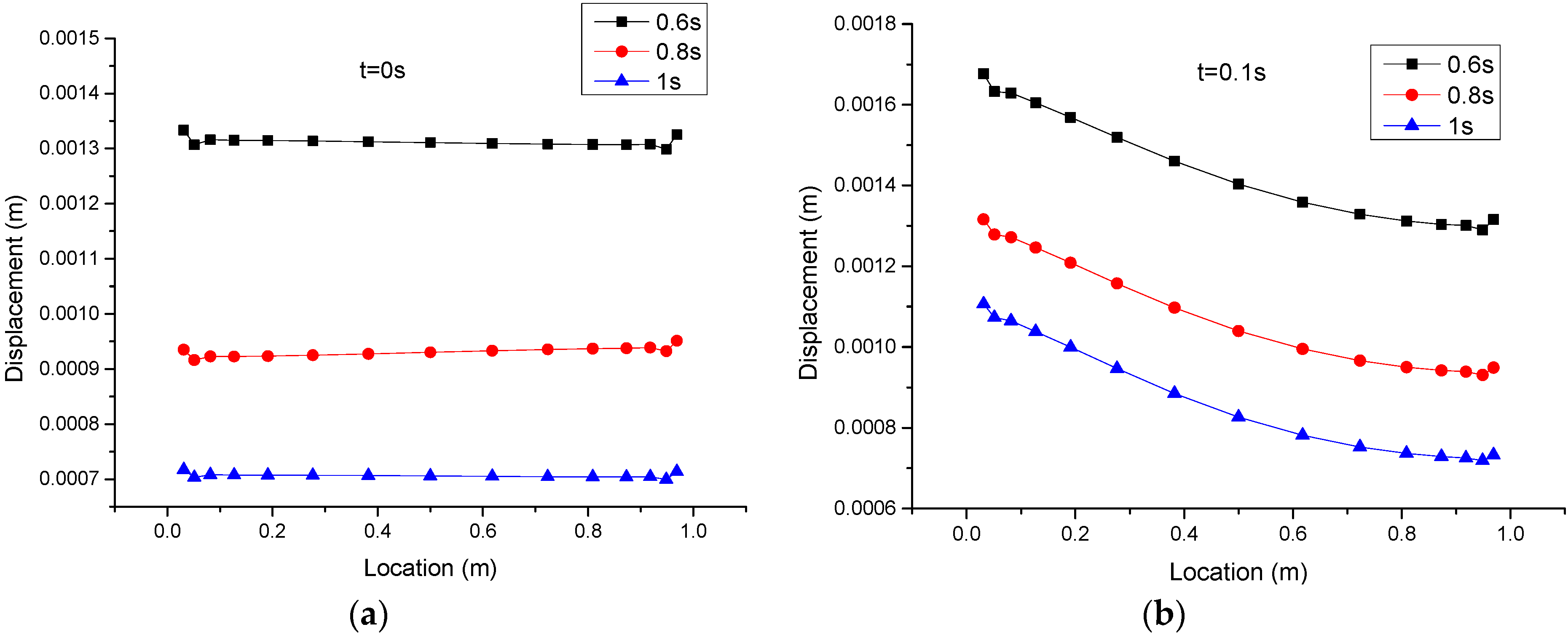
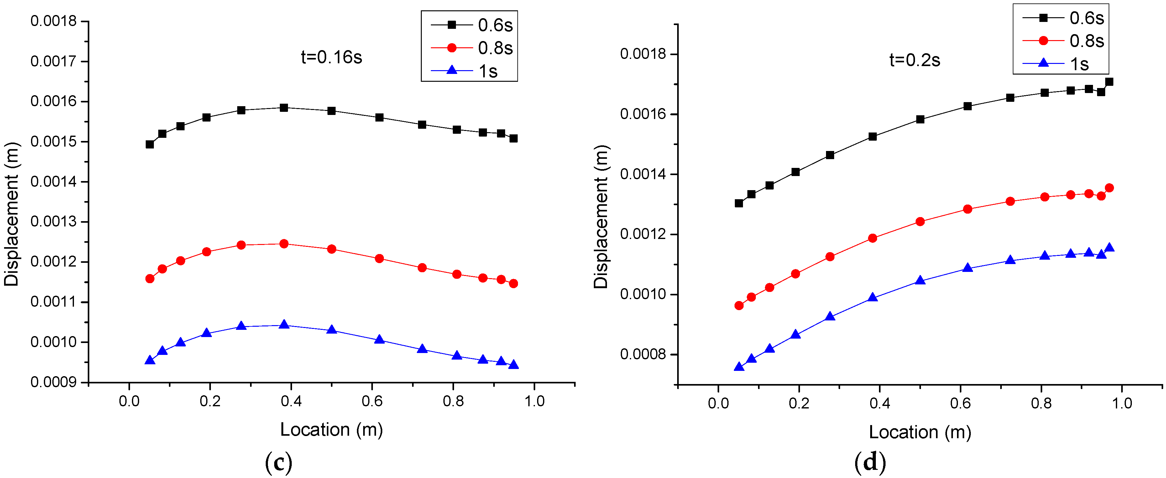
Secondly, this paper analyzed the changes of tube displacement under different cardiac cycles. In
Figure 12, three lines represent the tube displacement circumstances in the three examples, with cardiac cycles of 0.6 s, 0.8 s, and 1 s.
Figure 12a shows the initial displacement circumstance of tube at 0 s.
Figure 12b shows the circumstance of tube displacement at 0.1 s, when the peak occurred at the inlet.
Figure 12c shows the circumstance of tube displacement at 0.16 s, when the peak had not reached the outlet.
Figure 12d shows the displacement circumstance at 0.2 s, when the peak reached the outlet. It can be seen that when the cardiac cycle decreased, tube wall deformation increased markedly, and
vice versa. The inlet pressure reached its peak value at 0.1 s. The pressure peak moved forward at 0.16 s and arrived at the outlet at 0.2 s. However, like the pressure distribution, the curve shape changed little under different frequencies. This illustrates that the cardiac cycle has limited influence on the change of flow in the tube, and the pressure change is mainly caused by a change in the fluid amount stored through tube wall deformation.
Figure 12.
Comparison of tube wall deformation under different cardiac cycle lengths: (a) 0 s; (b) 0.1 s; (c) 0.16 s; (d) 0.2 s.
Figure 12.
Comparison of tube wall deformation under different cardiac cycle lengths: (a) 0 s; (b) 0.1 s; (c) 0.16 s; (d) 0.2 s.
With the coupling effect of three major systems, the proposed model successfully simulated the pressure changes in the tube only by adjusting cardiac cycle length. The simulated pressure changes have been proved to accord with the actual physiological features. This illustrates that the model of this paper is a well-developed and reliable system, which is able to show comprehensively the transition process of the circulation system under different states.
4. Conclusions
Conclusively, the liquid-solid coupling hemodynamic model built in this paper considering microcirculation load effect is able to effectively simulate pulse wave propagation and reflection. It can also reflect the physiological features of human aortas and circulation system. The model is a hemodynamic model according with actual physiological process. Through data analysis, it was revealed that in the human blood circulation system, the coupling relationship of liquid, solid, and porous media seepage is exactly the deep reason why the various complex flowing phenomena of human blood occur in the circulation process. The effects of the propagation and reflection of the pulse wave should not be ignored in hemodynamic simulations. Meanwhile, through this model, we were able to simulate the motion and physiological features of flow in a blood vessel more rationally. This study thus provides an important theoretical foundation and technical methods for analyzing cause, development, and clinical treatment of atherosclerosis, aneurysms, high blood pressure, and other cardiovascular and cerebrovascular diseases in the future.
The constitutive equation of microcirculation load has a great influence on the bloodstream, and has decisive influence on various phenomena in the flow field. Therefore, in hemodynamic study and simulation, the influence of microcirculation load must be considered. The simulations will achieve a better correspondence with human physiology through deep study of microcirculation load properties and improving the constitutive equation of the model.
The model is able to realize the transition of the circulation system under different flow field conditions, providing the possibility of simulating the dynamic condition of the human circulation system. Through studying dynamic properties, we cannot only analyze the properties of the blood circulation system under different physiological states, but also simulate the transition process of the human body between different physiological states. These have important meanings for research on aneurysms and other blood diseases.
However, the present work is limited by physiological inaccuracies in the geometrical shape of the models. Further work will be conducted on the simulation in actual arterial geometries extracted from CT angiography or MRI. High-precision grids will be employed. In addition, the effect of non-Newtonian fluid on the small arteries will be considered.


