
A Review of Time-Scale Modification of Music Signals †

International Audio Laboratories Erlangen, 91058 Erlangen, Germany
*
Authors to whom correspondence should be addressed.
†
This paper is an extended version of our paper published in the Proceedings of the International Conference on Digital Audio Effects (DAFx), Erlangen, Germany, 1–5 September 2014.
‡
These authors contributed equally to this work.
Appl. Sci. 2016, 6(2), 57; https://0-doi-org.brum.beds.ac.uk/10.3390/app6020057
Submission received: 22 December 2015
/
Revised: 22 January 2016
/
Accepted: 25 January 2016
/
Published: 18 February 2016
(This article belongs to the Special Issue Audio Signal Processing)
Abstract
:Time-scale modification (TSM) is the task of speeding up or slowing down an audio signal’s playback speed without changing its pitch. In digital music production, TSM has become an indispensable tool, which is nowadays integrated in a wide range of music production software. Music signals are diverse—they comprise harmonic, percussive, and transient components, among others. Because of this wide range of acoustic and musical characteristics, there is no single TSM method that can cope with all kinds of audio signals equally well. Our main objective is to foster a better understanding of the capabilities and limitations of TSM procedures. To this end, we review fundamental TSM methods, discuss typical challenges, and indicate potential solutions that combine different strategies. In particular, we discuss a fusion approach that involves recent techniques for harmonic-percussive separation along with time-domain and frequency-domain TSM procedures.
1. Introduction
Time-scale modification (TSM) procedures are digital signal processing methods for stretching or compressing the duration of a given audio signal. Ideally, the time-scale modified signal should sound as if the original signal’s content was performed at a different tempo while preserving properties like pitch and timbre. TSM procedures are applied in a wide range of scenarios. For example, they simplify the process of creating music remixes. Music producers or DJs apply TSM to adjust the durations of music recordings, enabling synchronous playback [1,2]. Nowadays TSM is built into music production software as well as hardware devices. A second application scenario is adjusting an audio stream’s duration to that of a given video clip. For example, when generating a slow motion video, it is often desirable to also slow down the tempo of the associated audio stream. Here, TSM can be used to synchronize the audio material with the video’s visual content [3].
A main challenge for TSM procedures is that music signals are complex sound mixtures, consisting of a wide range of different sounds. As an example, imagine a music recording consisting of a violin playing together with castanets. When modifying this music signal with a TSM procedure, both the harmonic sound of the violin as well as the percussive sound of the castanets should be preserved in the output signal. To keep the violin’s sound intact, it is essential to maintain its pitch as well as its timbre. On the other hand, the clicking sound of the castanets does not have a pitch—it is much more important to maintain the crisp sound of the single clicks, as well as their exact relative time positions, in order to preserve the original rhythm. Retaining these contrasting characteristics usually requires conceptually different TSM approaches. For example, classical TSM procedures based on waveform similarity overlap-add (WSOLA) [4] or on the phase vocoder (PV-TSM) [5,6,7] are capable of preserving the perceptual quality of harmonic signals to a high degree, but introduce noticeable artifacts when modifying percussive signals. However, it is possible to substantially reduce artifacts by combining different TSM approaches. For example, in [8], a given audio signal is first separated into a harmonic and a percussive component. Afterwards, each component is processed with a different TSM procedure that preserves its respective characteristics. The final output signal is then obtained by superimposing the two intermediate output signals.
Our goals in this article are two-fold. First, we aim to foster an understanding of fundamental challenges and algorithmic approaches in the field of TSM by reviewing well-known TSM methods and discussing their respective advantages and drawbacks in detail. Second, having identified the core issues of these classical procedures, we show—through an example—how to improve on them by combining different algorithmic ideas. We begin the article by introducing a fundamental TSM strategy as used in many TSM procedures (Section 2) and discussing a simple TSM approach based on overlap-add (Section 3). Afterwards, we review two conceptually different TSM methods: the time-domain WSOLA (Section 4) as well as the frequency-domain PV-TSM (Section 5). We then review the state-of-the-art TSM procedure from [8] that improves on the quality of both WSOLA as well as PV-TSM by incorporating harmonic-percussive separation (Section 6). Finally, we point out different application scenarios for TSM (such as music synchronization and pitch-shifting), as well as various freely available TSM implementations (Section 7).
2. Fundamentals of Time-Scale Modification (TSM)
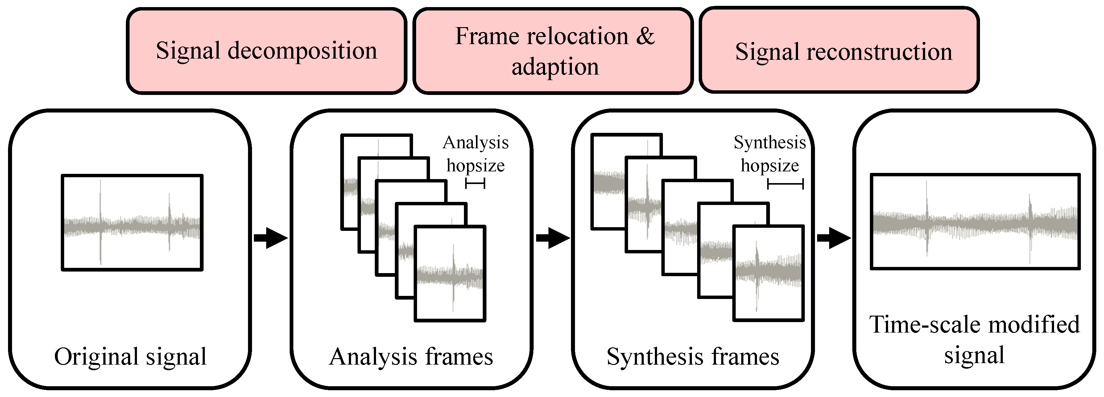
As mentioned above, a key requirement for time-scale modification procedures is that they change the time-scale of a given audio signal without altering its pitch content. To achieve this goal, many TSM procedures follow a common fundamental strategy which is sketched in Figure 1. The core idea is to decompose the input signal into short frames. Having a fixed length, usually in the range of 50 to 100 milliseconds of audio material, each frame captures the local pitch content of the signal. The frames are then relocated on the time axis to achieve the actual time-scale modification, while, at the same time, preserving the signal’s pitch.
More precisely, this process can be described as follows. The input of a TSM procedure is a discrete-time audio signal , equidistantly sampled at a sampling rate of . Note that although audio signals typically have a finite length of samples for , for the sake of simplicity, we model them to have an infinite support by defining for . The first step of the TSM procedure is to split x into short analysis frames , , each of them having a length of N samples (in the literature, the analysis frames are sometimes also referred to as grains, see [9]). The analysis frames are spaced by an analysis hopsize :
In a second step, these frames are relocated on the time axis with regard to a specified synthesis hopsize . This relocation accounts for the actual modification of the input signal’s time-scale by a stretching factor . Since it is often desirable to have a specific overlap of the relocated frames, the synthesis hopsize is often fixed (common choices are or ) while the analysis hopsize is given by . However, simply superimposing the overlapping relocated frames would lead to undesired artifacts such as phase discontinuities at the frame boundaries and amplitude fluctuations. Therefore, prior to signal reconstruction, the analysis frames are suitably adapted to form synthesis frames . In the final step, the synthesis frames are superimposed in order to reconstruct the actual time-scale modified output signal of the TSM procedure:
Although this fundamental strategy seems straightforward at a first glance, there are many pitfalls and design choices that may strongly influence the perceptual quality of the time-scale modified output signal. The most obvious question is how to adapt the analysis frames in order to form the synthesis frames . There are many ways to approach this task, leading to conceptually different TSM procedures. In the following, we discuss several strategies.
3. TSM Based on Overlap-Add (OLA)
3.1. The Procedure
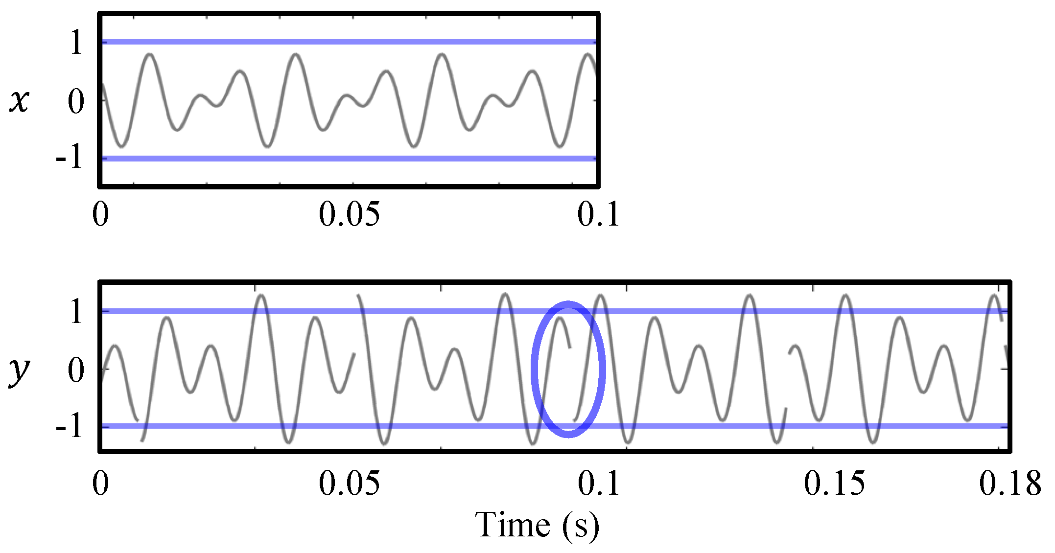
In the general scheme described in the previous section, a straightforward approach would be to simply define the synthesis frames to be equal to the unmodified analysis frames . This strategy, however, immediately leads to two problems which are visualized in Figure 2. First, when reconstructing the output signal by using Equation (2), the resulting waveform typically shows discontinuities—perceivable as clicking sounds—at the unmodified frames’ boundaries. Second, the synthesis hopsize is usually chosen such that the synthesis frames are overlapping. When superimposing the unmodified frames—each of them having the same amplitude as the input signal—this typically leads to an undesired increase of the output signal’s amplitude.
A basic TSM procedure should both enforce a smooth transition between frames as well as compensate for unwanted amplitude fluctuations. The idea of the overlap-add (OLA) TSM procedure is to apply a window function w to the analysis frames, prior to the reconstruction of the output signal y. The task of the window function is to remove the abrupt waveform discontinuities at the the analysis frames’ boundaries. A typical choice for w is a Hann window function
The Hann window has the nice property that
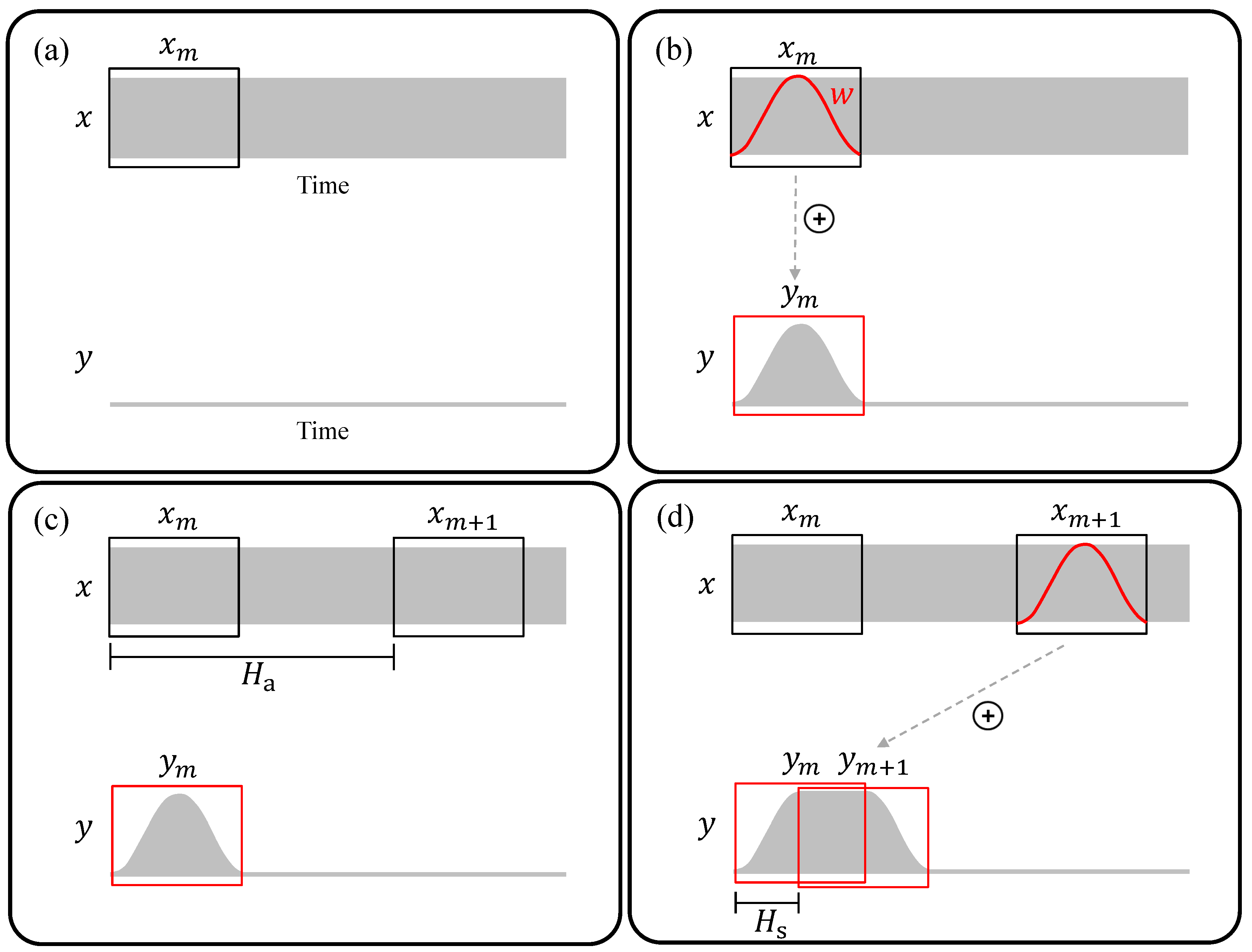
for all . The principle of the iterative OLA procedure is visualized in Figure 3. For the frame index , we first use Equation (1) to compute the analysis frame (Figure 3a). Then, we derive the synthesis frame by
The nominator of Equation (5) constitutes the actual windowing of the analysis frame by multiplying it pointwise with the given window function. The denominator normalizes the frame by the sum of the overlapping window functions, which prevents amplitude fluctuations in the output signal. Note that, when choosing w to be a Hann window and , the denominator always reduces to one by Equation (4). This is the case in Figure 3b where the synthesis frame’s amplitude is not scaled before being added to the output signal y. Proceeding to the next analysis frame , (Figure 3c), this frame is again windowed, overlapped with the preceding synthesis frame, and added to the output signal (Figure 3d). Note that Figure 3 visualizes the case where the original signal is compressed (). Stretching the signal () works in exactly the same fashion. In this case, the analysis frames overlap to a larger degree than the synthesis frames.
OLA is an example of a time-domain TSM procedure where the modifications to the analysis frames are applied purely in the time-domain. In general, time-domain TSM procedures are not only efficient but also preserve the timbre of the input signal to a high degree. On the downside, output signals produced by OLA often suffer from other artifacts, as we explain next.
3.2. Artifacts
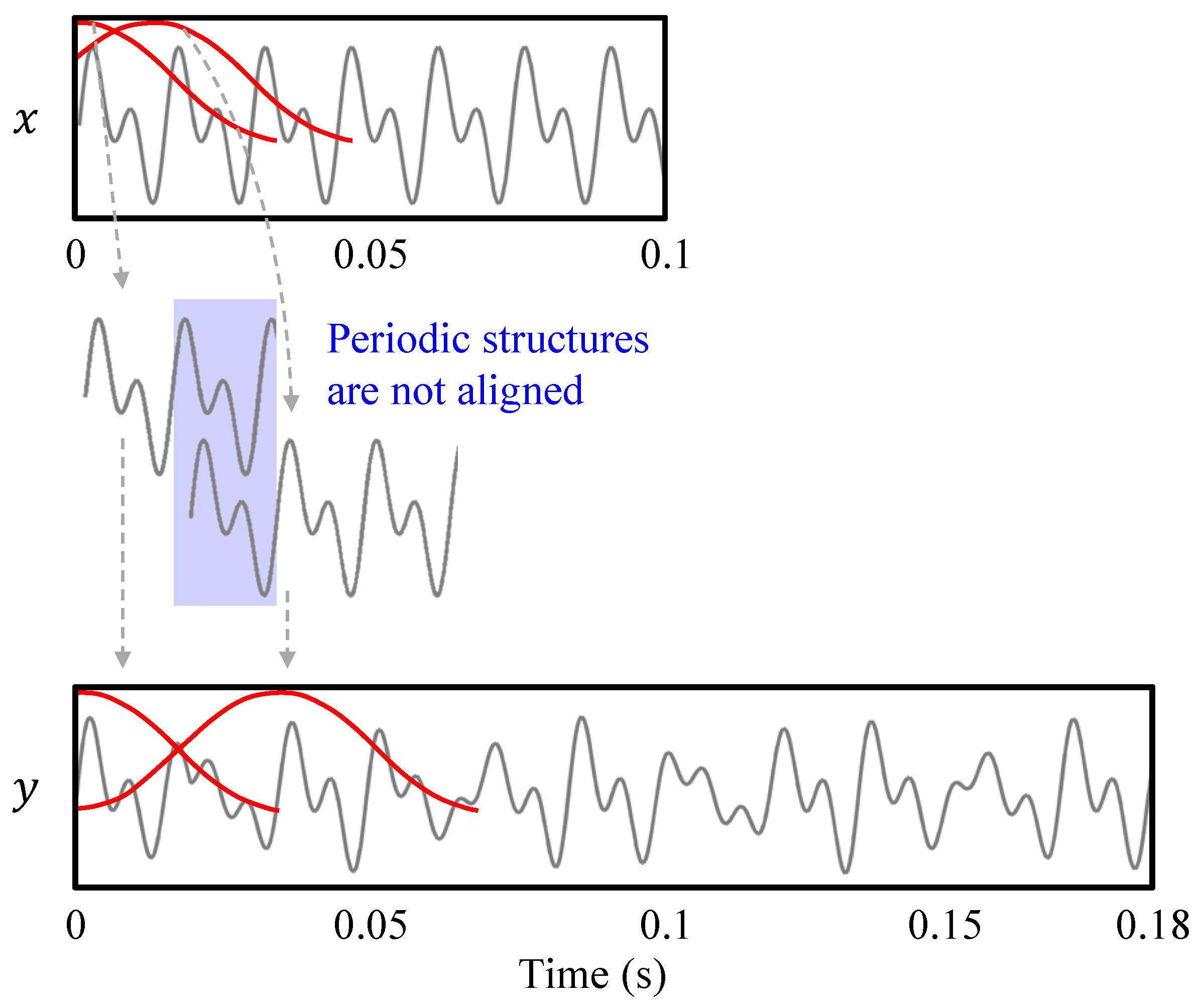
The OLA procedure is in general not capable of preserving local periodic structures that are present in the input signal. This is visualized in Figure 4 where a periodic input signal x is stretched by a factor of using OLA. When relocating the analysis frames, the periodic structures of x may not align any longer in the superimposed synthesis frames. In the resulting output signal y, the periodic patterns are distorted. These distortions are also known as phase jump artifacts. Since local periodicities in the waveforms of audio signals correspond to harmonic sounds, OLA is not suited to modify signals that contain harmonic components. When applied to harmonic signals, the output signals of OLA have a characteristic warbling sound, which is a kind of periodic frequency modulation [6]. Since most music signals contain at least some harmonic sources (as for example singing voice, piano, violins, or guitars), OLA is usually not suited to modify music.
3.3. Tricks of the Trade
While OLA is unsuited for modifying audio signals with harmonic content, it delivers high quality results for purely percussive signals, as is the case with drum or castanet recordings [8]. This is because audio signals with percussive content seldom have local periodic structures. The phase jump artifacts introduced by OLA are therefore not noticeable in the output signals. In this scenario, it is important to choose a very small frame length N (corresponding to roughly 10 milliseconds of audio material) in order to reduce the effect of transient doubling, an artifact that we discuss at length in Section 4.2.
4. TSM Based on Waveform Similarity Overlap-Add (WSOLA)
4.1. The Procedure
One of OLA’s problems is that it lacks signal sensitivity: the windowed analysis frames are copied from fixed positions in the input signal to fixed positions in the output signal. In other words, the input signal has no influence on the procedure. One time-domain strategy to reduce phase jump artifacts as caused by OLA is to introduce some flexibility in the TSM process, achieved by allowing some tolerance in the analysis or synthesis frames’ positions. The main idea is to adjust successive synthesis frames in such a way that periodic structures in the frames’ waveforms are aligned in the overlapping regions. Periodic patterns in the input signal are therefore maintained in the output. In the literature, several variants of this idea have been described, such as synchronized OLA (SOLA) [10], time-domain pitch-synchronized OLA (TD-PSOLA) [11], or autocorrelation-based approaches [12].
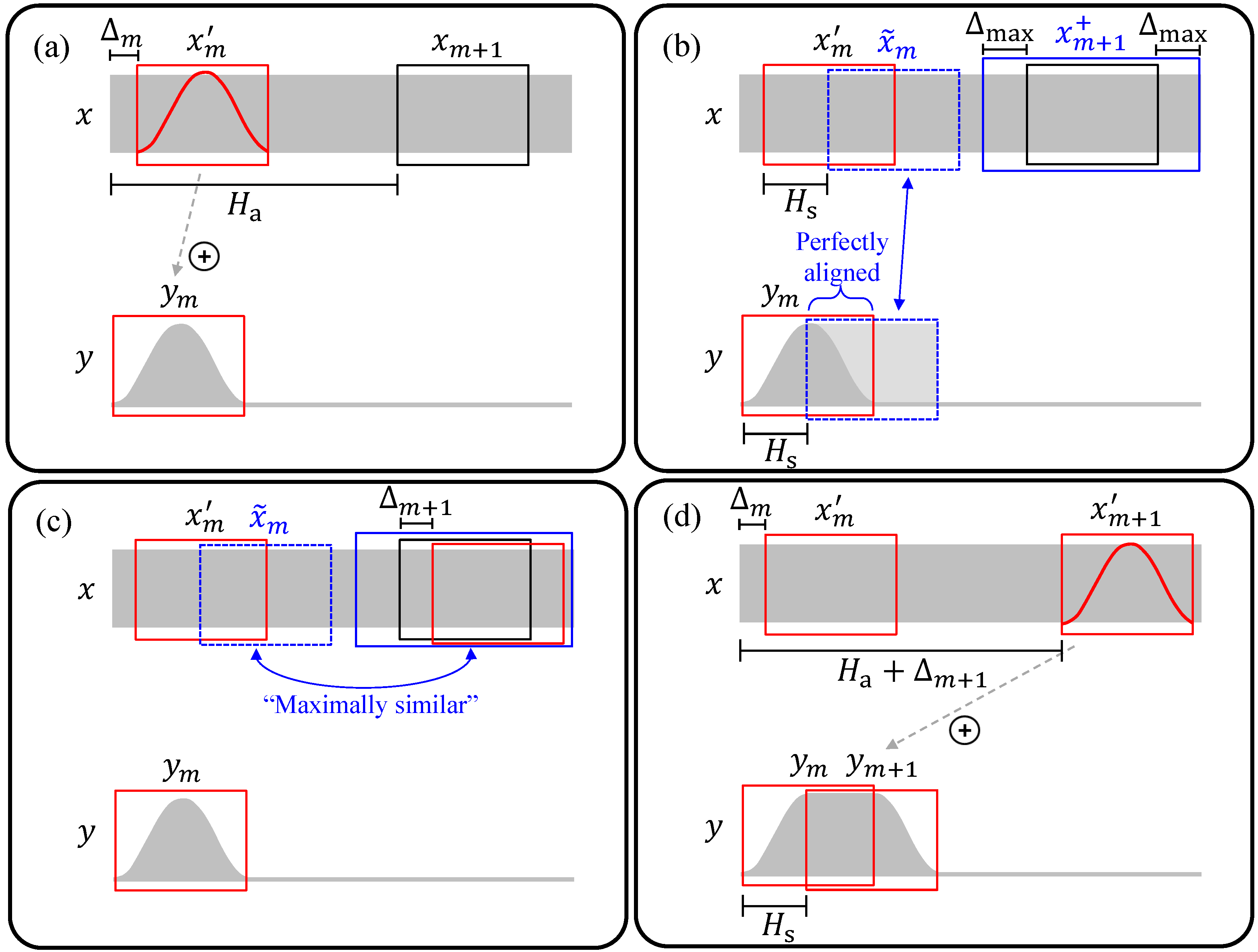
Another well-known procedure is waveform similarity-based OLA (WSOLA) [4]. This method’s core idea is to allow for slight shifts (of up to samples) of the analysis frames’ positions. Figure 5 visualizes the principle of WSOLA. Similar to OLA, WSOLA proceeds in an iterative fashion. Assume that in the iteration the position of the analysis frame was shifted by samples. We call this frame the adjusted analysis frame (Figure 5a):
The adjusted analysis frame is windowed and copied to the output signal y as in OLA (Figure 5a). Now, we need to adjust the position of the next analysis frame . This task can be interpreted as a constrained optimization problem. Our goal is to find the optimal shift index such that periodic structures of the adjusted analysis frame are optimally aligned with structures of the previously copied synthesis frame in the overlapping region when superimposing both frames at the synthesis hopsize . The natural progression of the adjusted analysis frame (dashed blue box in Figure 5b) would be an optimal choice for the adjusted analysis frame in an unconstrained scenario:
This is the case, since the adjusted analysis frame and the synthesis frame are essentially the same (up to windowing). As a result, the structures of the natural progression are perfectly aligned with the structures of the synthesis frame when superimposing the two frames at the synthesis hopsize (Figure 5b). However, due to the constraint , the adjusted frame must be located inside of the extended frame region (solid blue box in Figure 5b):
Therefore, the idea is to retrieve the adjusted frame as the frame in whose waveform is most similar to . To this end, we must define a measure that quantifies the similarity of two frames. One possible choice for this metric is the cross-correlation
of a signal q and a signal p shifted by samples. We can then compute the optimal shift index that maximizes the cross-correlation of and by
The shift index defines the position of the adjusted analysis frame inside the extended frame region (Figure 5c). Finally, we compute the synthesis frame , similarly to OLA, by
and use Equation (2) to reconstruct the output signal y (Figure 5d). In practice, we start the iterative optimization process at the frame index and assume .
4.2. Artifacts
WSOLA can improve on some of the drawbacks of OLA as illustrated by Figure 6 (WSOLA) and Figure 4 (OLA). However, it still causes certain artifacts that are characteristic for time-domain TSM procedures.
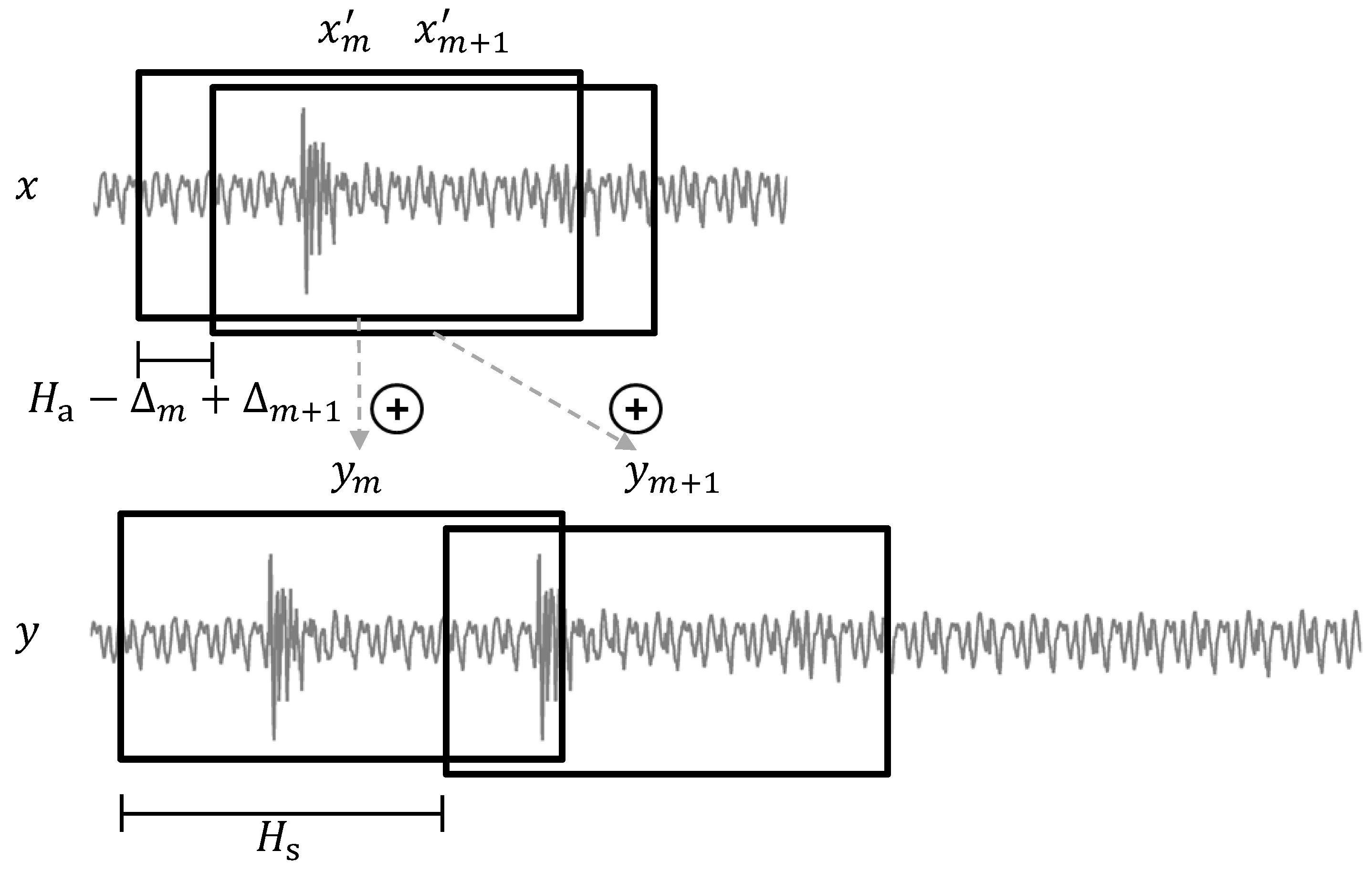
A prominent problem with WSOLA-like methods is known as transient doubling or stuttering. This artifact is visualized in Figure 7, where we can see a single transient in the input signal x that is contained in the overlapping region of two successive adjusted analysis frames and . When the frames are relocated and copied to the output signal, the transient is duplicated and can be heard two times in quick succession. A related artifact is transient skipping where transients get lost in the modification process since they are not contained in any of the analysis frames. While transient doubling commonly occurs when stretching a signal (), transient skipping usually happens when the signal is compressed (). These artifacts are particularly noticeable when modifying signals with percussive components, such as recordings of instruments with strong onsets (e.g., drums, piano).
Furthermore, WSOLA has particular problems when modifying polyphonic input signals such as recordings of orchestral music. For these input signals, the output often still contains considerable warbling. The reason for this is that WSOLA can, by design, only preserve the most prominent periodic pattern in the input signal’s waveform. Therefore, when modifying recordings with multiple harmonic sound sources, only the sound of the most dominant source is preserved in the output, whereas the remaining sources can still cause phase jump artifacts. While WSOLA is well-suited to modify monophonic input signals, this is often not the case with more complex audio.
4.3. Tricks of the Trade
In order to assure that WSOLA can adapt to the most dominant periodic pattern in the waveform of the input signal, one frame must be able to capture at least a full period of the pattern. In addition, the tolerance parameter must be large enough to allow for an appropriate adjustment. Therefore, it should be set to at least half a period’s length. Assuming that the lowest frequency that can be heard by humans is roughly 20 Hz, a common choice is a frame length N corresponding to 50 ms and a tolerance parameter of 25 ms.
One possibility to reduce transient doubling and skipping artifacts in WSOLA is to apply a transient preservation scheme. In [13], the idea is to first identify the temporal positions of transients in the input signal by using a transient detector. Then, in the WSOLA process, the analysis hopsize is temporarily fixed to be equal to the synthesis hopsize whenever an analysis frame is located in a neighborhood of an identified transient. This neighborhood, including the transient, is therefore copied without modification to the output signal, preventing WSOLA from doubling or skipping it. The deviation in the global stretching factor is compensated dynamically in the regions between transients.
5. TSM Based on the Phase Vocoder (PV-TSM)
5.1. Overview
As we have seen, WSOLA is capable of maintaining the most prominent periodicity in the input signal. The next step to improve the quality of time-scale modified signals is to preserve the periodicities of all signal components. This is the main idea of frequency-domain TSM procedures, which interpret each analysis frame as a weighted sum of sinusoidal components with known frequency and phase. Based on these parameters, each of these components is manipulated individually to avoid phase jump artifacts across all frequencies in the reconstructed signal.
A fundamental tool for the frequency analysis of the input signal is the short-time Fourier transform [14] (Section 5.2). However, depending on the chosen discretization parameters, the resulting frequency estimates may be inaccurate. To this end, the phase vocoder (Although the term “phase vocoder” refers to a specific technique for the estimation of instantaneous frequencies, it is also frequently used in the literature as the name of the TSM procedure itself.) technique [5,7] is used to improve on the the short-time Fourier transform’s coarse frequency estimates by deriving the sinusoidal components’ instantaneous frequencies (Section 5.3). In TSM procedures based on the phase vocoder (PV-TSM), these improved estimates are used to update the phases of an input signal’s sinusoidal components in a process known as phase propagation (Section 5.4).
5.2. The Short-Time Fourier Transform
The most important tool of PV-TSM is the short-time Fourier transform (STFT), which applies the Fourier transform to every analysis frame of a given input signal. The STFT X of a signal x is given by
where is the frame index, is the frequency index, N is the frame length, is the analysis frame of x as defined in Equation (1), and w is a window function. Given the input signal’s sampling rate , the frame index m of is associated to the physical time
given in seconds, and the frequency index k corresponds to the physical frequency
given in Hertz. The complex number , also called a time-frequency bin, denotes the Fourier coefficient for the analysis frame. It can be represented by a magnitude and a phase as
The magnitude of an STFT X is also called a spectrogram which is denoted by Y:
In the context of PV-TSM, it is necessary to reconstruct the output signal y from a modified STFT . Note that a modified STFT is in general not invertible [15]. In other words, there might be no signal y that has as its STFT. However, there exist methods that aim to reconstruct a signal y from whose STFT is close to with respect to some distance measure. Following the procedure described in [16], we first compute time-domain frames by using the inverse Fourier transform.
5.3. The Phase Vocoder
Each time-frequency bin of an STFT can be interpreted as a sinusoidal component with amplitude and phase that contributes to the analysis frame of the input signal x. However, the Fourier transform yields coefficients only for a discrete set of frequencies that are sampled linearly on the frequency axis, see Equation (14). The STFT’s frequency resolution therefore does not suffice to assign a precise frequency value to this sinusoidal component. The phase vocoder is a technique that refines the STFT’s coarse frequency estimate by exploiting the given phase information.
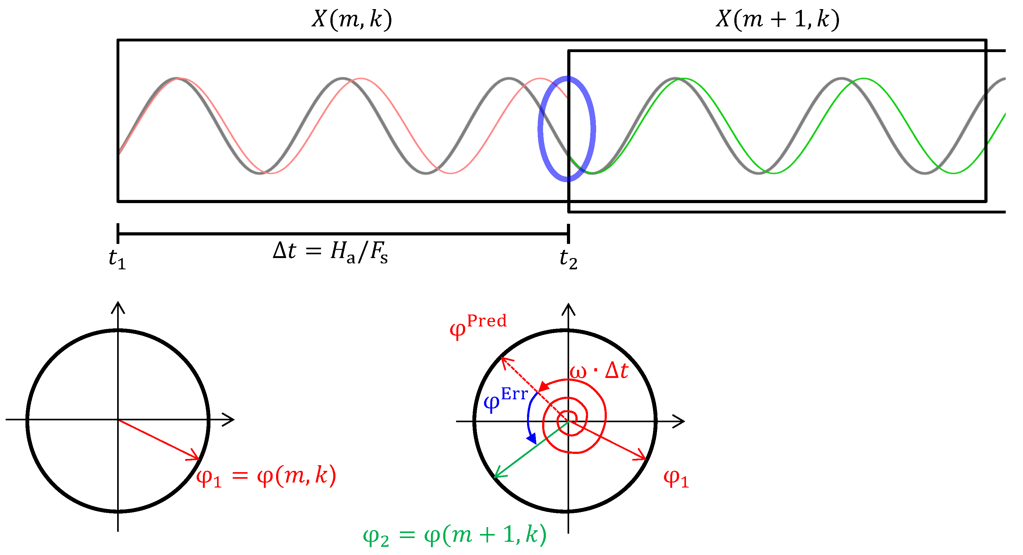
In order to understand the phase vocoder, let us have a look at the scenario shown in Figure 8. Assume we are given two phase estimates and at the time instances and of a sinusoidal component for which we only have a coarse frequency estimate . Our goal is to estimate the sinusoid’s “real” instantaneous frequency . Figure 8 shows this sinusoidal component (gray) as well as two sinusoids that have a frequency of ω (red and green). In addition, we also see phase representations at the time instances and . The red sinusoid has a phase of at and the green sinusoid a phase of at . One can see that the frequency ω of the red and green sinusoids is slightly lower than the frequency of the gray sinusoid. Intuitively, while the phases of the gray and the red sinusoid match at , they diverge over time, and we can observe a considerable discrepancy after seconds (blue oval). Since we know the red sinusoid’s frequency, we can compute its unwrapped phase advance, i.e., the number of oscillations that occur over the course of seconds:
Knowing that its phase at is , we can predict its phase after seconds:
At we again have a precise phase estimate for the gray sinusoid. We therefore can compute the phase error (also called the heterodyned phase increment [17]) between the phase actually measured at and the predicted phase when assuming a frequency of ω:
where Ψ is the principal argument function that maps a given phase into the range . Note that by mapping into this range, we assume that the number of oscillations of the gray and red sinusoids differ by at most half a period. In the context of instantaneous frequency estimation, this means that the coarse frequency estimate ω needs to be close to the actual frequency of the sinusoid, and that the interval should be small. The unwrapped phase advance of the gray sinusoid can then be computed by the sum of the unwrapped phase advance of the red sinusoid with frequency ω (red spiral arrow) and the phase error (blue curved arrow):
This gives us the number of oscillations of the gray sinusoid over the course of seconds. From this we can derive the instantaneous frequency of the gray sinusoid by
The frequency can be interpreted as the small offset of the gray sinusoid’s actual frequency from the rough frequency estimate ω.
We can use this approach to refine the coarse frequency resolution of the STFT by computing instantaneous frequency estimates for all time-frequency bins :
with , (the analysis hopsize given in seconds), , and . For further details, we refer to ([15], Chapter 8).
5.4. PV-TSM
The principle of PV-TSM is visualized in Figure 9. Given an input audio signal x, the first step of PV-TSM is to compute the STFT X. Figure 9a depicts the two successive frequency spectra of the and analysis frames, denoted by and , respectively (here, a frame’s Fourier spectrum is visualized as a set of sinusoidals, representing the sinusoidal components that are captured in the time-frequency bins). Our goal is to compute a modified STFT with adjusted phases from which we can reconstruct a time-scale modified signal without phase jump artifacts:
We compute the adjusted phases in an iterative process that is known as phase propagation. Assume that the phases of the frame have already been modified (see the red sinusoid’s phase in Figure 9b being different from its phase in Figure 9a). As indicated by Figure 9b, overlapping the and frame at the synthesis hopsize may lead to phase jumps. Knowing the instantaneous frequencies derived by the phase vocoder, we can predict the phases of the sinusoidal components in the frame after a time interval corresponding to samples. To this end, we set , , and (the synthesis hopsize given in seconds) in Equation (20). This allows us to replace the phases of the frame with the predicted phase:
for . Assuming that the estimates of the instantaneous frequencies are correct, there are no phase jumps any more when overlapping the modified spectra at the synthesis hopsize (Figure 9c). In practice, we start the iterative phase propagation with the frame index and set
for all . Finally, the output signal y can be computed using the signal reconstruction procedure described in Section 5.2 (Figure 9d).
5.5. Artifacts
By design, PV-TSM can achieve phase continuity for all sinusoidal components contributing to the output signal. This property, also known as horizontal phase coherence, ensures that there are no artifacts related to phase jumps. However, the vertical phase coherence, i.e., the phase relationships of sinusoidal components within one frame, is usually destroyed in the phase propagation process. The loss of vertical phase coherence affects the time localization of events such as transients. As a result, transients are often smeared in signals modified with PV-TSM (Figure 10). Furthermore, output signals of PV-TSM commonly have a very distinct sound coloration known as phasiness [18], an artifact also caused by the loss of vertical phase coherence. Signals suffering from phasiness are described as being reverberant, having “less bite,” or a “loss of presence” [6].
5.6. Tricks of the Trade
The phase vocoder technique highly benefits from frequency estimates that are already close to the instantaneous frequencies as well as from a small analysis hopsize (resulting in a small ). In PV-TSM, the frame length N is therefore commonly set to a relatively large value. In practice, N typically corresponds to roughly 100 ms in order to achieve a high frequency resolution of the STFT.
To reduce the loss of vertical phase coherence in the phase vocoder, Laroche and Dolson proposed a modification to the standard PV-TSM in [6]. Their core observation is that a sinusoidal component may affect multiple adjacent time-frequency bins of a single analysis frame. Therefore, the phases of these bins should not be updated independently, but in a joint fashion. A peak in a frame’s magnitude spectrum is assumed to be representative of a particular sinusoidal component. The frequency bins with lower magnitude values surrounding the peak are assumed to be affected by the same component as well. In the phase propagation process, only the time-frequency bins with a peak magnitude are updated in the usual fashion described in Equation (26). The phases of the remaining frequency bins are locked to the phase of the sinusoidal component corresponding to the closest peak. This procedure allows to locally preserve the signal’s vertical phase coherence. This technique, also known as identity phase locking, leads to reduced phasiness artifacts and less smearing of transients.
Another approach to reduce phasieness artifacts is the phase vocoder with synchronized overlap-add (PVSOLA) and similar formulations [19,20,21]. The core observation of these methods is that the original vertical phase coherence is usually lost gradually over the course of phase-updated synthesis frames. Therefore, these procedures “reset” the vertical phase coherence repeatedly after a fixed number of frames. The resetting is done by copying an analysis frame unmodified to the output signal and adjusting it in a WSOLA-like fashion. After having reset the vertical phase coherence, the next synthesis frames are again computed by the phase propagation strategy.
To reduce the effect of transient smearing, other approaches include transient preservation schemes, similar to those for WSOLA. In [22], transients are identified in the input signal, cut out from the waveform, and temporarily stored. The remaining signal, after filling the gaps using linear prediction techniques, is modified using PV-TSM. Finally, the stored transients are relocated according to the stretching factor and reinserted into the modified signal.
6. TSM Based on Harmonic-Percussive Separation
6.1. The Procedure
As we have seen in the previous sections, percussive sound components and transients in the input signal cause issues with WSOLA and PV-TSM. On the other hand, OLA is capable of modifying percussive and transient sounds rather well, while causing phase jump artifacts in harmonic signals. The idea of a recent TSM procedure proposed in [8] is to combine PV-TSM and OLA in order to modify both harmonic and percussive sound components with high quality. The procedure’s principle is visualized in Figure 11. The shown input signal consists of a tone played on a violin (harmonic) superimposed with a single click of castanets halfway through the signal (percussive). The first step is to decompose the input signal into two sound components: a harmonic component and a percussive component. This is done by using a harmonic-percussive separation (HPS) technique. A simple and effective method for this task was proposed by Fitzgerald in [23], which we review in Section 6.2. As we can see in Figure 11, the harmonic component captures the violin’s sound while the percussive component contains the castanets’ click. A crucial observation is that the harmonic component usually does not contain percussive residues and vice versa. After having decomposed the input signal, the idea of [8] is to apply PV-TSM with identity phase locking (see Section 5.6) to the harmonic component and OLA with a very short frame length (see Section 3.3) to the percussive component. By treating the two components independently with the two different TSM procedures, their respective characteristics can be preserved to a high degree. Finally, the superposition of the two modified signal components forms the output of the procedure. A conceptually similar strategy for TSM has been proposed by Verma and Meng in [24] where they use a sines+transients+noise signal model [25,26,27,28] to parameterize a given signal’s sinusoidal, transient, and noise-like sound components. The estimated parameters are then modified in order to synthesize a time-scaled output signal. However, their procedure relies on an explicit transient detection in order to estimate appropriate parameters for the transient sound components.
In contrast to other transient preserving TSM procedures such as [13,22,24,29], the approach based on HPS has the advantage that an explicit detection and preservation of transients is not necessary. Figure 12 shows the same input signal x as in Figure 10. Here, the signal is stretched by a factor of using TSM based on HPS. Unlike Figure 10, the transient from the input signal x is also clearly visible in the output signal y. When looking closely, one can see that the transient is actually doubled by OLA (Section 4.2). However, due to the short frame length used in the procedure, the transient repeats so quickly that the doubling is not noticeable when listening to the output signal. The TSM procedure based on HPS was therefore capable of preserving the transient without an explicit transient detection. Since both the explicit detection and preservation of transients are non-trivial and error-prone tasks, the achieved implicit transient preservation yields a more robust TSM procedure. The TSM approach based on HPS is therefore a good example of how the strengths of different TSM procedures can be combined in a beneficial way.
6.2. Harmonic-Percussive Separation
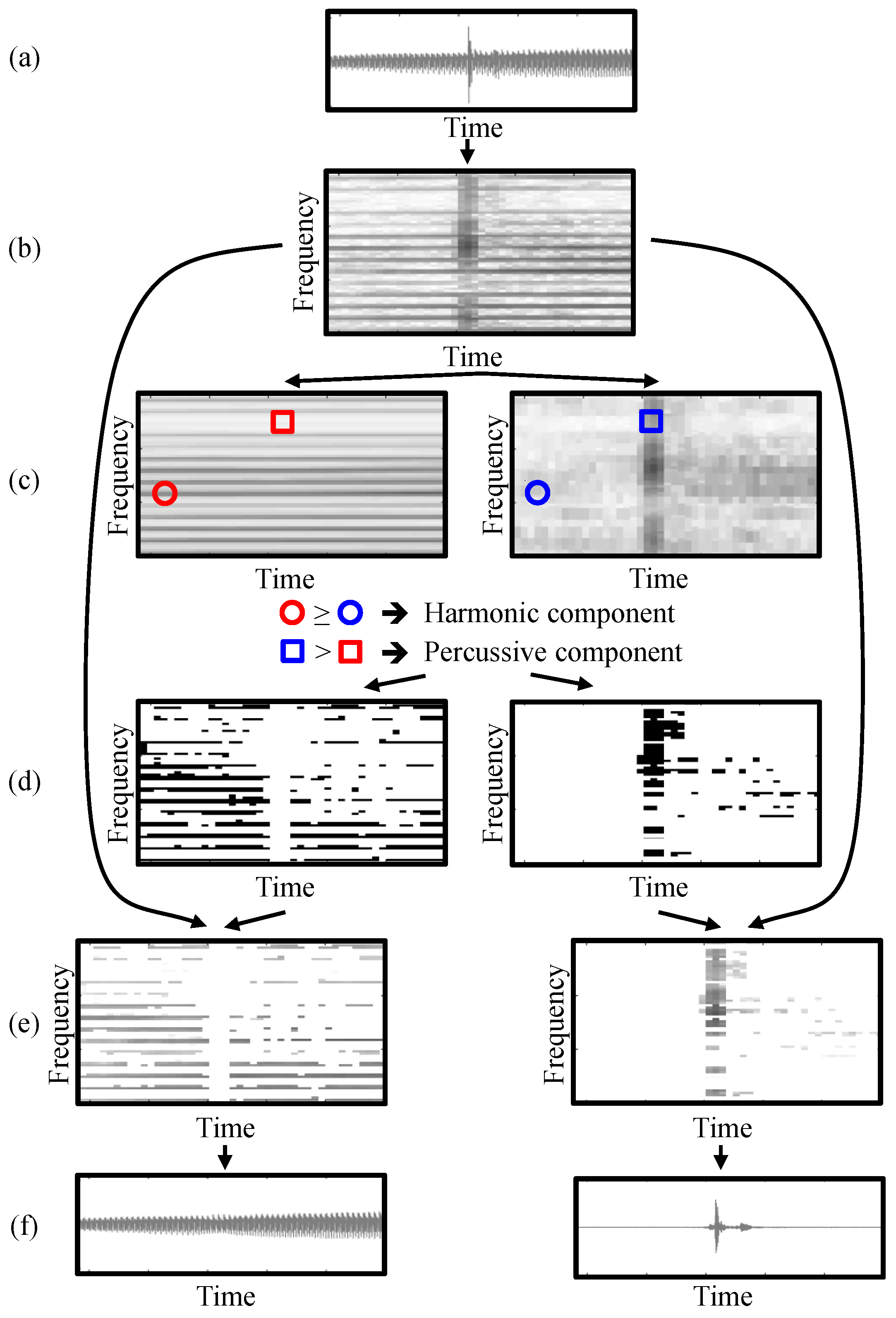
The goal of harmonic-percussive separation (HPS) is to decompose a given audio signal x into a signal consisting of all harmonic sound components and a signal consisting of all percussive sound components. While there exist numerous approaches for this task [30,31,32,33,34,35], a particularly simple and effective method was proposed by Fitzgerald in [23], which we review in the following. To illustrate the procedure, let us have a look at Figure 13. The input is an audio signal as shown in Figure 13a. Here, we again revert to our example of a tone played on the violin, superimposed with a single click of castanets. The first step is to compute the STFT X of the given audio signal x as defined in Equation (15). A critical observation is that, in the spectrogram , harmonic sounds form structures in the time direction, while percussive sounds yield structures in the frequency direction. In the spectrogram shown in Figure 13b we can see horizontal lines, reflecting the harmonic sound of the violin, as well as a single vertical line in the middle of the spectrogram, stemming from a click of the castanets. By applying a median filter to Y—once horizontally and once vertically—we get a horizontally enhanced spectrogram and a vertically enhanced spectrogram :
for , where and are the lengths of the median filters, respectively (Figure 13c). We assume a time-frequency bin of the original STFT to be part of the harmonic component if and of the percussive component if . Using this principle, we can define binary masks and for the harmonic and the percussive components (Figure 13d):
Applying these masks to the original STFT X yields modified STFTs corresponding to the harmonic and percussive components (Figure 13e):
These modified STFTs can then be transformed back to the time-domain by using the reconstruction strategy discussed in Section 5.2. This yields the desired signals and , respectively. As we can see in Figure 13f, the harmonic component contains the tone played by the violin, while the percussive component shows the waveform of the castanets’ click.
7. Applications
7.1. Music Synchronization—Non-Linear TSM
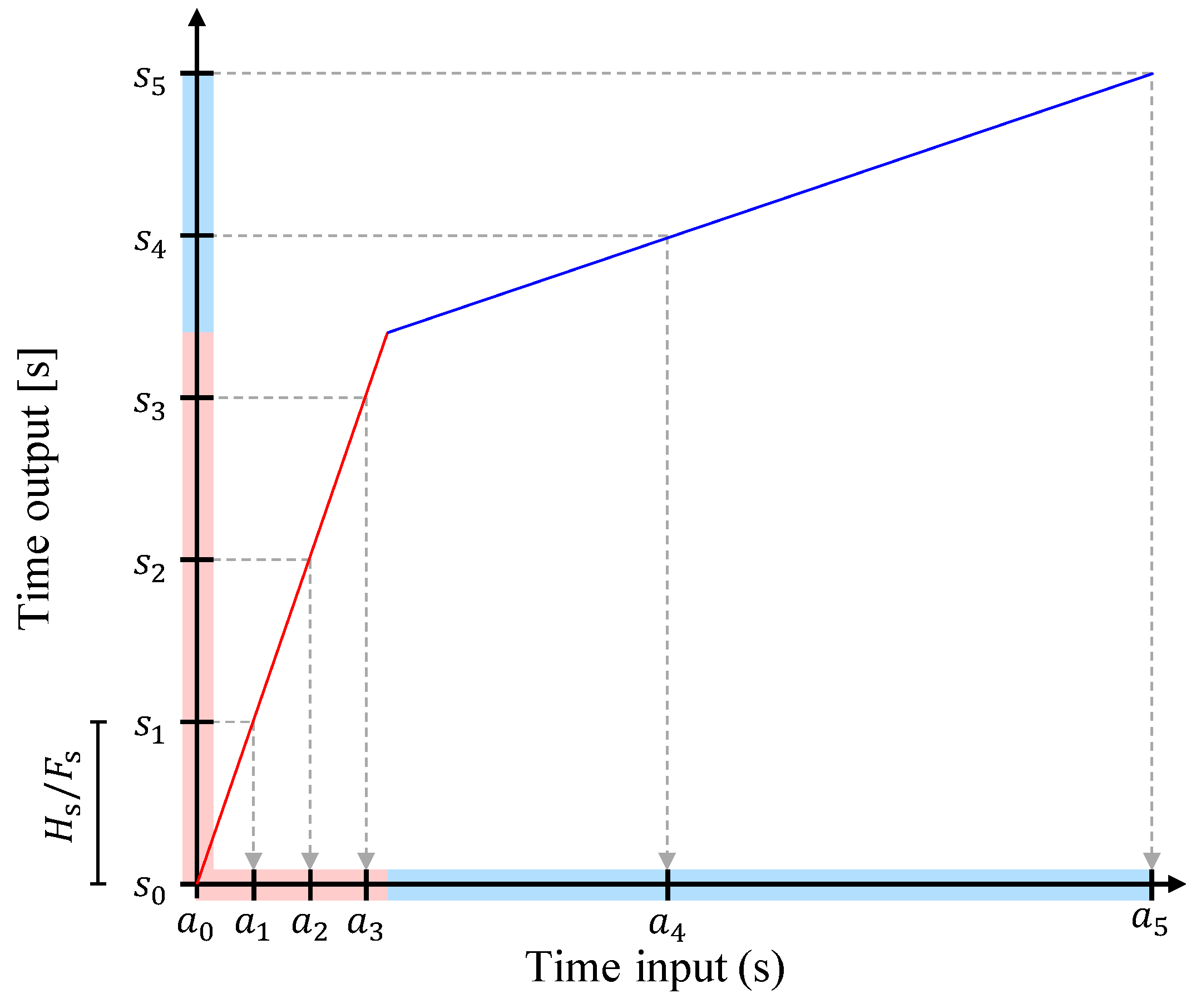
In scenarios like automated soundtrack generation [36] or automated DJing [1,2], it is often necessary to synchronize two or more music recordings by aligning musically related beat positions in time. However, music recordings do not necessarily have a constant tempo. In this case, stretching or compressing the recordings by a constant factor α is insufficient to align their beat positions. Instead, the recordings’time-scales need to be modified in a non-linear fashion. The goal of non-linear TSM is to modify an audio signal according to a strictly monotonously increasing time-stretch function , which defines a mapping between points in time (given in seconds) of the input and output signals. Figure 14 shows an example of such a function. The first part, shown in red, has a slope greater than one. As a consequence, the red region in the input signal is mapped to a larger region in the output, resulting in a stretch. The slope of the function’s second part, shown in blue, is smaller than one, leading to a compression of this region in the output. One possibility to realize this kind of non-linear modifications is to define the positions of the analysis frames according to the time-stretch function τ, instead of a constant analysis hopsize . The process of deriving the analysis frames’ positions is presented in Figure 14. Given τ, we first fix a synthesis hopsize as we did for linear TSM (see Section 2). From this, we derive the synthesis instances (given in seconds), which are the positions of the synthesis frames in the output signal:
By inverting τ, we compute the analysis instances (given in seconds):
When using analysis frames indicated by the analysis instances for TSM with a procedure of our choice, the resulting output signal is modified according to the time-stretch function τ. To this end, all of the previously discussed TSM procedures can also be used for non-linear TSM.
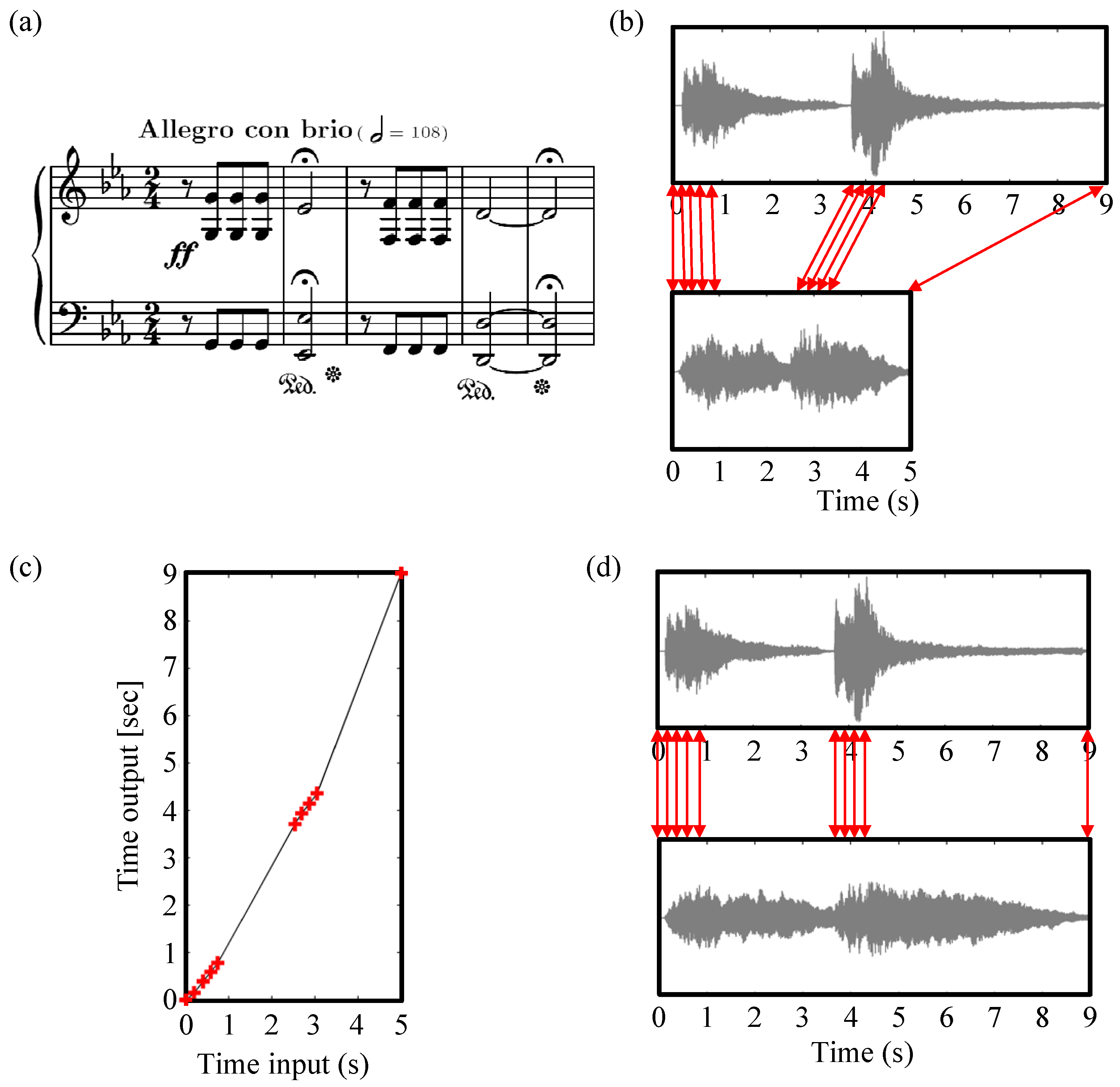
A very convenient way of defining a time-stretch function is by introducing a set of anchor points. An anchor point is a pair of time positions where the first entry specifies a time position in the input signal and the second entry is a time position in the output signal. The actual time-stretch function τ is then obtained by a linear interpolation between the anchor points. Figure 15 shows a real-world example of a non-linear modification. In Figure 15b, we see the waveforms of two recorded performances of the first five measures of Beethoven’s Symphony No. 5. The corresponding time positions of the note onsets are indicated by red arrows. Obviously, the first recording is longer than the second. However, the performances’ tempi do not differ by a constant factor. While the eighth notes in the first and third measure are played at almost the same tempo in both performances, the durations of the half notes (with fermata) in measures two and five are significantly longer in the first recording. The mapping between the note onsets of the two performances is therefore non-linear. In Figure 15c, we define eight anchor points that map the onset positions of the second performance to the onset positions of the first performance (plus two additional anchor points aligning the recordings’ start times and end times, respectively). Based on these anchor points and the derived time-stretch function τ, we then apply the TSM procedure of our choice to the second performance in order to obtain a version that is onset-synchronized with the first performance (Figure 15d).
7.2. Pitch-Shifting
Pitch-shifting is the task of changing an audio recording’s pitch without altering its length—it can be seen as the dual problem to TSM. While there are specialized pitch-shifting procedures [37,38], it is also possible to approach the problem by combining TSM with resampling. The core observation is that resampling a given signal and playing it back at the original sampling rate changes the length and the pitch of the signal at the same time (The same effect can be simulated with vinyl records by changing the rotation speed of the record player). To pitch-shift a given signal, it is therefore first resampled and afterwards time-scale modified in order to compensate for the change in length. More precisely, an audio signal, sampled at a rate of , is first resampled to have a new sampling rate of . When playing back the signal at its original sampling rate , this operation changes the signal’s length by a factor of and scales its frequencies by the term’s inverse. For example, musically speaking, a factor of increases the pitch content by one octave. To compensate for the change in length, the signal needs to be stretched by a factor of , using a TSM procedure.
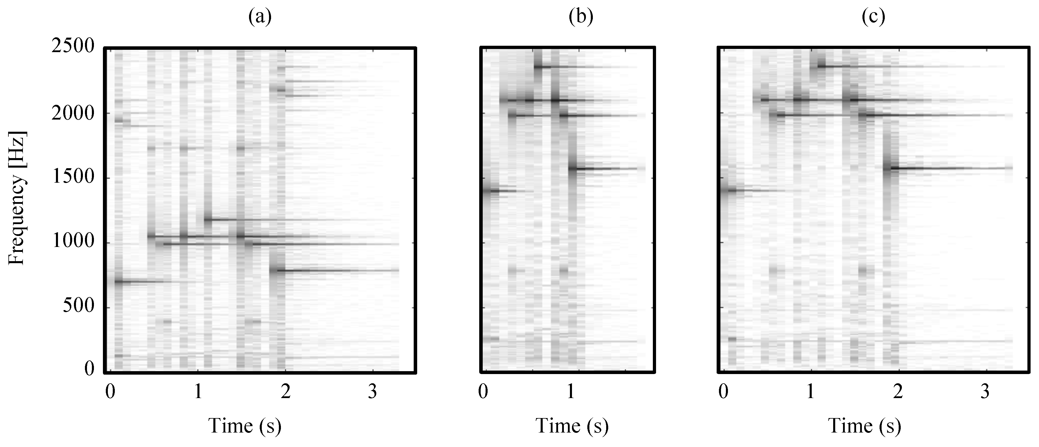
To demonstrate this, we show an example in Figure 16, where the goal is to apply a pitch-shift of one octave to the input audio signal. The original signal has a sampling rate of Hz (Figure 16a). To achieve the desired pitch-shift, the signal is resampled to Hz (Figure 16b). One can see that the resampling changed the pitch of the signal as well as its length when interpreting the signal as still being sampled at Hz. While the change in pitch is desired, the change in length needs to be compensated for. Thus, we stretch the signal by a factor of to its original length (Figure 16c).
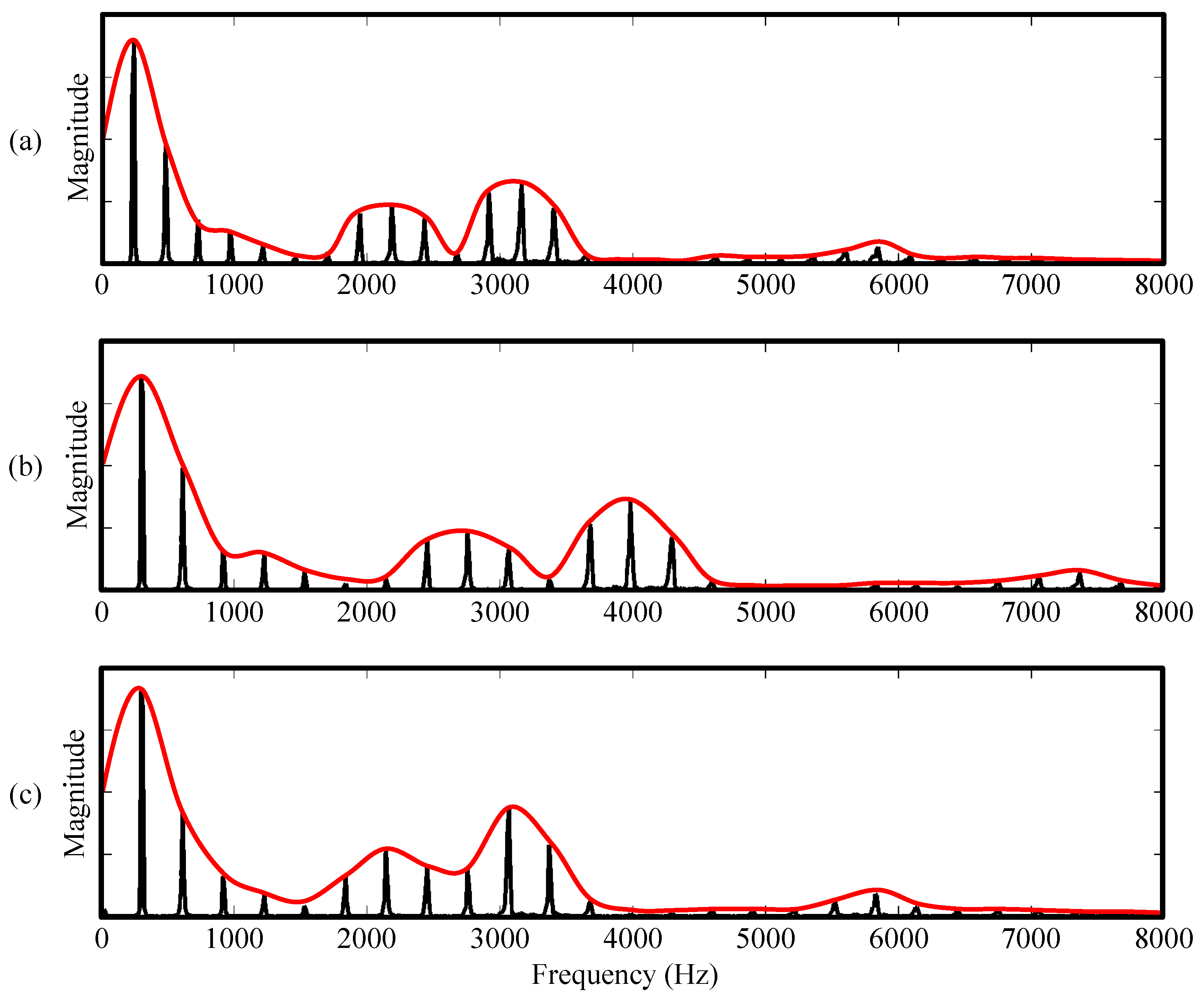
The quality of the pitch-shifting result crucially depends on various factors. First, artifacts that are produced by the applied TSM procedure are also audible in the pitch-shifted signal. However, even when using a high-quality TSM procedure, the pitch-shifted signals generated by the method described above often sound unnatural. For example, when pitch-shifting singing voice upwards by several semitones, the modified voice has an artificial sound, sometimes referred to as the chipmunk effect [39]. Here, the problem is that the spectral envelope, which is the rough shape of a frequency spectrum, is of central importance for the timbre of a sound. In Figure 17a, we see a frame’s frequency spectrum from a singing voice recording. Due to the harmonic nature of the singing voice, the spectrum shows a comb-like pattern where the energy is distributed at multiples of a certain frequency—in this example roughly 250 Hz. The peaks in the pattern are called the harmonics of the singing voice. The magnitudes of the harmonics follow a certain shape which is specified by the spectral envelope (marked in red). Peaks in the spectral envelope are known as formants. In the example from Figure 17a, we see four formants at around 200 Hz, 2200 Hz, 3100 Hz, and 5900 Hz. The frequency positions of these formants are closely related to the singing voice’s timbre. In Figure 17b, we see the spectrum of the same frame after being pitch-shifted by four semitones with the previously described pitch-shifting procedure. Due to the resampling, the harmonics’ positions are scaled. The spectral envelope is therefore scaled as well, relocating the positions of the formants. This leads to a (usually undesired) change in timbre of the singing voice.
One strategy to compensate for this change is outlined in [17]. Let X and be the STFTs of a given input signal x and its pitch-shifted version , respectively. Fixing a frame index m, let and be the frequency spectra of the frames in X and . Furthermore, let and denote the spectral envelopes of and , respectively. Our goal is to compute modified spectra that have the frequency content of but the original spectral envelopes . To this end, we normalize the magnitudes of with respect to its spectral envelope and then scale them by the original envelope :
In Figure 17c we see the frame’s spectrum from Figure 17b after the envelope adaption, leading to a signal that sounds more natural.
There exist several approaches to estimate spectral envelopes, many of them either based on linear predictive coding (LPC) [40] or on the cepstrum (the inverse Fourier transform of the logarithmic magnitude spectrum) [41,42]. Generally, the task of spectral envelope estimation is highly complex and error-prone. In envelope or formant-preserving pitch-shifting methods, it is often necessary to manually specify parameters (e.g., the pitch range of the sources in the recording) to make the envelope estimation more robust.
7.3. Websources
Various free implementations of TSM procedures are available in different programming languages. MATLAB implementations of OLA, WSOLA, PV-TSM, and TSM based on HPS, as well as additional test and demo material can be found in the TSM Toolbox [43,44]. A further MATLAB implementation of PV-TSM can be found at [45]. PV-TSM implemented in Python is included in LibROSA [46]. Furthermore, there are open source C/C++ audio processing libraries that offer TSM functionalities. For example, the Rubber Band Library [47] includes a transient preserving PV-TSM and the SoundTouch Audio Processing Library [48] offers a WSOLA-like TSM procedure. Finally, there also exist proprietary commercial implementations such as the élastique algorithm by zplane [49].
8. Conclusions
In this article, we reviewed time-scale modification of music signals. We presented fundamental principles and discussed various well-known time and frequency-domain TSM procedures. Additionally, we pointed out more involved procedures proposed in the literature, which are—to varying extents—based on the fundamental approaches we reviewed. In particular, we discussed a recent approach that involves harmonic-percussive separation and combines the advantages of two fundamental TSM methods in order to attenuate artifacts and improve the quality of time-scale modified signals. Finally, we introduced some applications of TSM, including music synchronization and pitch-shifting, and gave pointers to freely available TSM implementations.
A major goal of this contribution was to present fundamental concepts in the field of TSM. Beyond discussing technical details, our main motivation was to give illustrative explanations in a tutorial-like style. Furthermore, we aimed to foster a deep understanding of the strengths and weaknesses of the various TSM approaches by discussing typical artifacts and the importance of parameter choices. We hope that this work constitutes a good starting point for becoming familiar with the field of TSM and developing novel TSM techniques.
Acknowledgments
This work has been supported by the German Research Foundation (DFG MU 2686/6-1). The International Audio Laboratories Erlangen are a joint institution of the Friedrich-Alexander-Universität Erlangen-Nürnberg (FAU) and Fraunhofer Institut für Integrierte Schaltungen. We also would like to thank Patricio López-Serrano for his careful proofreading and comments on the article.
Author Contributions
The authors contributed equally to this work. The choice of focus, didactical preparation of the material, design of the figures, as well as writing the paper were all done in close collaboration.
Conflicts of Interest
The authors declare no conflict of interest.
References
- Cliff, D. Hang the DJ: Automatic Sequencing and Seamless Mixing of Dance-Music Tracks; Technical Report; HP Laboratories Bristol: Bristol, Great Britain, 2000. [Google Scholar]
- Ishizaki, H.; Hoashi, K.; Takishima, Y. Full-automatic DJ mixing system with optimal tempo adjustment based on measurement function of user discomfort. In Proceedings of the International Society for Music Information Retrieval Conference (ISMIR), Kobe, Japan, 26–30 October 2009; pp. 135–140.
- Moinet, A.; Dutoit, T.; Latour, P. Audio time-scaling for slow motion sports videos. In Proceedings of the International Conference on Digital Audio Effects (DAFx), Maynooth, Ireland, 2–5 September 2013.
- Verhelst, W.; Roelands, M. An overlap-add technique based on waveform similarity (WSOLA) for high quality time-scale modification of speech. In Proceedings of the IEEE International Conference on Acoustics, Speech, and Signal Processing (ICASSP), Minneapolis, MN, USA, 27–30 April 1993.
- Flanagan, J.L.; Golden, R.M. Phase vocoder. Bell Syst. Tech. J. 1966, 45, 1493–1509. [Google Scholar] [CrossRef]
- Laroche, J.; Dolson, M. Improved phase vocoder time-scale modification of audio. IEEE Trans. Speech Audio Process. 1999, 7, 323–332. [Google Scholar] [CrossRef]
- Portnoff, M.R. Implementation of the digital phase vocoder using the fast Fourier transform. IEEE Trans. Acoust. Speech Signal Process. 1976, 24, 243–248. [Google Scholar] [CrossRef]
- Driedger, J.; Müller, M.; Ewert, S. Improving time-scale modification of music signals using harmonic-percussive separation. IEEE Signal Process. Lett. 2014, 21, 105–109. [Google Scholar] [CrossRef]
- Zölzer, U. DAFX: Digital Audio Effects; John Wiley & Sons, Inc.: New York, NY, USA, 2002. [Google Scholar]
- Roucos, S.; Wilgus, A.M. High quality time-scale modification for speech. In Proceedings of the IEEE International Conference on Acoustics, Speech, and Signal Processing (ICASSP), Tampa, Florida, USA, 26–29 April 1985; Volume 10, pp. 493–496.
- Moulines, E.; Charpentier, F. Pitch-synchronous waveform processing techniques for text-to-speech synthesis using diphones. Speech Commun. 1990, 9, 453–467. [Google Scholar] [CrossRef]
- Laroche, J. Autocorrelation method for high-quality time/pitch-scaling. In Proceedings of the IEEE Workshop Applications of Signal Processing to Audio and Acoustics (WASPAA), Mohonk, NY, USA, 17–20 October 1993; pp. 131–134.
- Grofit, S.; Lavner, Y. Time-scale modification of audio signals using enhanced WSOLA with management of transients. IEEE Trans. Audio Speech Lang. Process. 2008, 16, 106–115. [Google Scholar] [CrossRef]
- Gabor, D. Theory of communication. J. Inst. Electr. Eng. IEE 1946, 93, 429–457. [Google Scholar] [CrossRef]
- Müller, M. Fundamentals of Music Processing; Springer International Publishing: Cham, Switzerland, 2015. [Google Scholar]
- Griffin, D.W.; Lim, J.S. Signal estimation from modified short-time Fourier transform. IEEE Trans. Acoust. Speech Signal Process. 1984, 32, 236–243. [Google Scholar] [CrossRef]
- Dolson, M. The phase vocoder: A tutorial. Comput. Music J. 1986, 10, 14–27. [Google Scholar] [CrossRef]
- Laroche, J.; Dolson, M. Phase-vocoder: About this phasiness business. In Proceedings of the IEEE ASSP Workshop on Applications of Signal Processing to Audio and Acoustics, New Paltz, NY, USA, 19–22 October 1997.
- Dorran, D.; Lawlor, R.; Coyle, E. A hybrid time-frequency domain approach to audio time-scale modification. J. Audio Eng. Soc. 2006, 54, 21–31. [Google Scholar]
- Kraft, S.; Holters, M.; von dem Knesebeck, A.; Zölzer, U. Improved PVSOLA time stretching and pitch shifting for polpyhonic audio. In Proceedings of the International Conference on Digital Audio Effects (DAFx), York, UK, 17–21 September 2012.
- Moinet, A.; Dutoit, T. PVSOLA: A phase vocoder with synchronized overlapp-add. In Proceedings of the International Conference on Digital Audio Effects (DAFx), Paris, France, 19–23 September 2011; pp. 269–275.
- Nagel, F.; Walther, A. A novel transient handling scheme for time stretching algorithms. In Proceedings of the AES Convention, New York, NY, USA, 2009; pp. 185–192.
- Fitzgerald, D. Harmonic/percussive separation using median filtering. In Proceedings of the International Conference on Digital Audio Effects (DAFx), Graz, Austria, 6–10 September 2010; pp. 246–253.
- Verma, T.S.; Meng, T.H. Time scale modification using a sines+transients+noise signal model. In Proceedings of the Digital Audio Effects Workshop (DAFx98), Barcelona, Spain, 19–21 November 1998.
- Levine, S. N.; Smith, J.O., III. A sines+transients+noise audio representation for data compression and time/pitch scale modications. In Proceedings of the AES Convention, Amsterdam, The Netherlands, 16–19 May 1998.
- Verma, T.S.; Meng, T.H. An analysis/synthesis tool for transient signals that allows a flexible sines+transients+noise model for audio. In Proceedings of the IEEE International Conference on Acoustics, Speech, and Signal Processing (ICASSP), Seattle, Washington, DC, USA, 12–15 May 1998; pp. 3573–3576.
- Verma, T.S.; Meng, T.H. Extending spectral modeling synthesis with transient modeling synthesis. Comput. Music J. 2000, 24, 47–59. [Google Scholar] [CrossRef]
- Serra, X.; Smith, J.O. Spectral modeling synthesis: A sound analysis/synthesis system based on a deterministic plus stochastic decomposition. Comput. Music J. 1990, 14, 12–24. [Google Scholar] [CrossRef]
- Duxbury, C.; Davies, M.; Sandler, M. Improved time-scaling of musical audio using phase locking at transients. In Proceedings of Audio Engineering Society Convention, Munich, Germany, 10–13 May 2002.
- Cañadas-Quesada, F.J.; Vera-Candeas, P.; Ruiz-Reyes, N.; Carabias-Orti, J.J.; Molero, P.C. Percussive/harmonic sound separation by non-negative matrix factorization with smoothness/sparseness constraints. EURASIP J. Audio Speech Music Process. 2014. [Google Scholar] [CrossRef]
- Duxbury, C.; Davies, M.; Sandler, M. Separation of transient information in audio using multiresolution analysis techniques. In Proceedings of the International Conference on Digital Audio Effects (DAFx), Limerick, Ireland, 17–22 September 2001.
- Gkiokas, A.; Papavassiliou, V.; Katsouros, V.; Carayannis, G. Deploying nonlinear image filters to spectrograms for harmonic/percussive separation. In Proceedings of the International Conference on Digital Audio Effects (DAFx), York, UK, 17–21 September 2012.
- Ono, N.; Miyamoto, K.; LeRoux, J.; Kameoka, H.; Sagayama, S. Separation of a monaural audio signal into harmonic/percussive components by complementary diffusion on spectrogram. In Proceedings of the European Signal Processing Conference, Lausanne, Switzerland, 25–29 August 2008; pp. 240–244.
- Park, J.; Lee, K. Harmonic-percussive source separation using harmonicity and sparsity constraints. In Proceedings of the International Conference on Music Information Retrieval (ISMIR), Málaga, Spain, 26–30 October 2015; pp. 148–154.
- Tachibana, H.; Ono, N.; Kameoka, H.; Sagayama, S. Harmonic/percussive sound separation based on anisotropic smoothness of spectrograms. IEEE/ACM Trans. Audio Speech Lang. Process. 2014, 22, 2059–2073. [Google Scholar] [CrossRef]
- Müller, M.; Driedger, J. Data-driven sound track generation. In Multimodal Music Processing; Müller, M., Goto, M., Schedl, M., Eds.; Schloss Dagstuhl–Leibniz-Zentrum für Informatik: Dagstuhl, Germany, 2012; Volume 3, pp. 175–194. [Google Scholar]
- Haghparast, A.; Penttinen, H.; Välimäki, V. Real-time pitch-shifting of musical signals by a time-varying factor using normalized filtered correlation time-scale modification. In Proceedings of the International Conference on Digital Audio Effects (DAFx), Bordeaux, France, 10–15 September 2007; pp. 7–14.
- Schörkhuber, C.; Klapuri, A.; Sontacchi, A. Audio pitch shifting using the constant-q transform. J. Audio Eng. Soc. 2013, 61, 562–572. [Google Scholar]
- Alvin and the Chipmunks—Recording Technique. Available online: https://en.wikipedia.org/wiki/Alvin_and_the_Chipmunks#Recording_technique (accessed on 3 December 2015).
- Markel, J.D.; Gray, A.H. Linear Prediction of Speech; Springer Verlag: Secaucus, NJ, USA, 1976. [Google Scholar]
- Röbel, A.; Rodet, X. Efficient spectral envelope estimation an its application to pitch shifting and envelope preservation. In Proceedings of the International Conference on Digital Audio Effects (DAFx), Madrid, Spain, 20–22 September 2005.
- Röbel, A.; Rodet, X. Real time signal transposition with envelope preservation in the phase vocoder. In Proceedings of the International Computer Music Conference (ICMC), Barcelona, Spain, 5–9 September 2005; pp. 672–675.
- Driedger, J.; Müller, M. TSM Toolbox. Available online: http://www.audiolabs-erlangen.de/resources/ matlab/pvoc/ (accessed on 5 February 2016).
- Driedger, J.; Müller, M. TSM Toolbox: MATLAB implementations of time-scale modification algorithms. In Proceedings of the International Conference on Digital Audio Effects (DAFx), Erlangen, Germany, 1–5 September 2014; pp. 249–256.
- Ellis, D.P.W. A Phase Vocoder in Matlab. Available online: http://www.ee.columbia.edu/dpwe/resources/ matlab/pvoc/ (accessed on 3 December 2015).
- McFee, B. Librosa—Time Stretching. Available online: https://bmcfee.github.io/librosa/generated/librosa.effects.time_stretch.html (accessed on 3 December 2015).
- Breakfast Quay. Rubber Band Library. Aailable online: http://breakfastquay.com/rubberband/ (accessed on 26 November 2015).
- Parviainen, O. Soundtouch Audio Processing Library. Available online: http://www.surina.net/soundtouch/ (accessed on 27 November 2015).
- Zplane Development. Élastique Time Stretching & Pitch Shifting SDKs. Available online: http://www.zplane.de/index.php?page=description-elastique (accessed on 5 February 2016).
Figure 1.
Generalized processing pipeline of Time-scale modification (TSM) procedures.

Figure 2.
Typical artifacts that occur when choosing the synthesis frames to be equal to the analysis frames . The input signal x is stretched by a factor of . The output signal y shows discontinuities (blue oval) and amplitude fluctuations (indicated by blue lines).
Figure 2.
Typical artifacts that occur when choosing the synthesis frames to be equal to the analysis frames . The input signal x is stretched by a factor of . The output signal y shows discontinuities (blue oval) and amplitude fluctuations (indicated by blue lines).

Figure 3.
The principle of TSM based on overlap-add (OLA). (a) Input audio signal x with analysis frame . The output signal y is constructed iteratively; (b) Application of Hann window function w to the analysis frame resulting in the synthesis frame ; (c) The next analysis frame having a specified distance of samples from ; (d) Overlap-add using the specified synthesis hopsize .

Figure 4.
Illustration of a typical artifact for an audio signal modified with OLA. In this example, the input signal x is stretched by a factor of . The OLA procedure is visualized for two frames indicated by window functions. The periodic structure of x is not preserved in the output signal y.
Figure 4.
Illustration of a typical artifact for an audio signal modified with OLA. In this example, the input signal x is stretched by a factor of . The OLA procedure is visualized for two frames indicated by window functions. The periodic structure of x is not preserved in the output signal y.

Figure 5.
The principle of Waveform Similarity Overlap-Add (WSOLA). (a) Input audio signal x with the adjusted analysis frame . The frame was already windowed and copied to the output signal y; (b,c) Retrieval of a frame from the extended frame region (solid blue box) that is as similar as possible to the natural progression (dashed blue box) of the adjusted analysis frame ; (d) The adjusted analysis frame is windowed and copied to the output signal y.

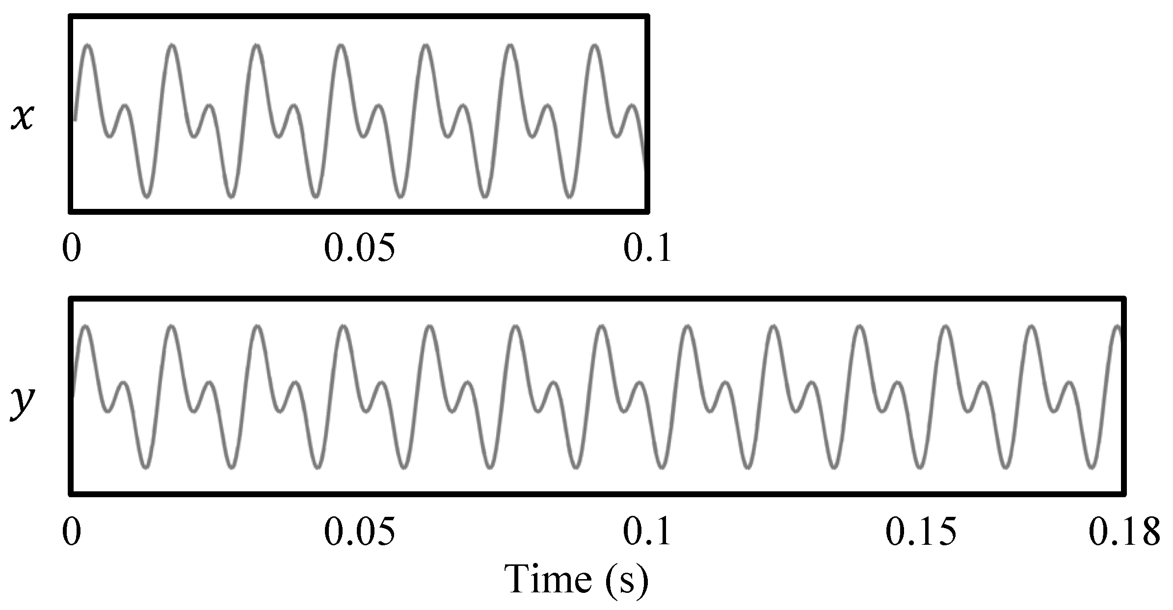
Figure 6.
Preservation of periodic structures by WSOLA. The input signal x is the same as in Figure 4, this time modified with WSOLA (time-stretch with ).
Figure 6.
Preservation of periodic structures by WSOLA. The input signal x is the same as in Figure 4, this time modified with WSOLA (time-stretch with ).

Figure 7.
Transient doubling artifact as it typically occurs in signals modified with WSOLA.

Figure 8.
Principle of the phase vocoder.

Figure 9.
The principle of TSM Based on the Phase Vocoder (PV-TSM). (a) STFT X (time-frequency bins are visualized by sinusoidals); (b) Using the original phase of leads to phase jumps when overlapping the frames at the synthesis hopsize (blue oval); (c) Update of the sinusoids’ phases via phase propagation. Phase jumps are reduced (blue oval); (d) Signal reconstruction from the modified STFT .

Figure 10.
Illustration of a smeared transient as a result of applying PV-TSM. The input signal x has been stretched by a factor of to yield the output signal y.
Figure 10.
Illustration of a smeared transient as a result of applying PV-TSM. The input signal x has been stretched by a factor of to yield the output signal y.

Figure 11.
Principle of TSM based on harmonic-percussive separation.

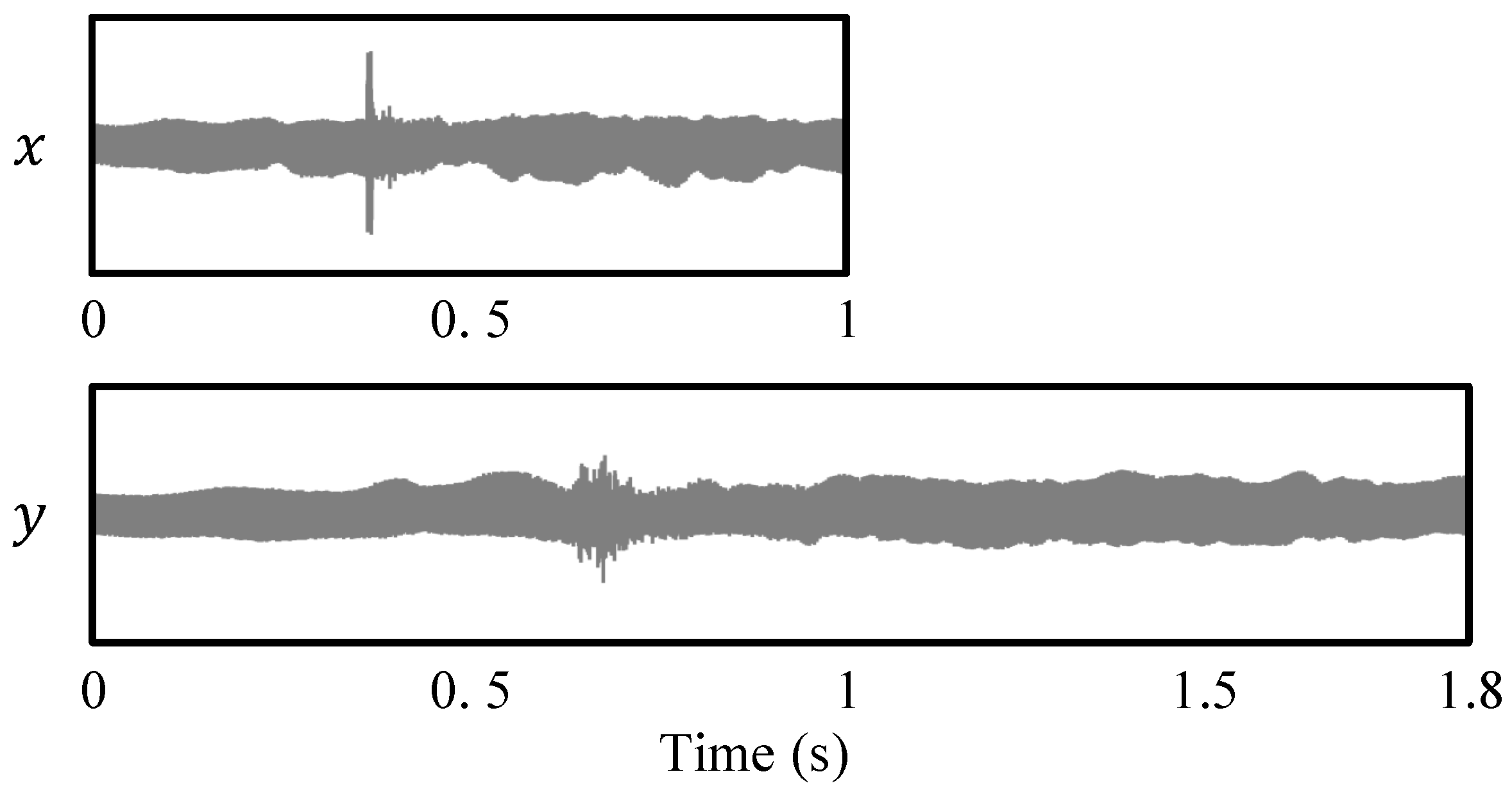
Figure 12.
Transient preservation in TSM based on harmonic-percussive separation (HPS). The input signal x is the same as in Figure 10 and is stretched by a factor of using TSM based on HPS.
Figure 12.
Transient preservation in TSM based on harmonic-percussive separation (HPS). The input signal x is the same as in Figure 10 and is stretched by a factor of using TSM based on HPS.

Figure 13.
The HPS procedure presented in [23]. (a) Input audio signal x; (b) STFT X of x; (c) Horizontally and vertically enhanced spectrograms and ; (d) Binary masks and ; (e) Spectrograms of the harmonic and the percussive component and ; (f) Harmonic and percussive components and .
Figure 13.
The HPS procedure presented in [23]. (a) Input audio signal x; (b) STFT X of x; (c) Horizontally and vertically enhanced spectrograms and ; (d) Binary masks and ; (e) Spectrograms of the harmonic and the percussive component and ; (f) Harmonic and percussive components and .

Figure 14.
Example of a non-linear time-stretch function τ.

Figure 15.
(a) Score of the first five measures of Beethoven’s Symphony No. 5; (b) Waveforms of two performances. Corresponding onset positions are indicated by red arrows; (c) Set of anchor points (indicated in red) and inferred time-stretch function τ; (d) Onset-synchronized waveforms of the two performances.

Figure 16.
Pitch-shifting via resampling and TSM. (a) Spectrogram of an input audio signal; (b) Spectrogram of the resampled signal; (c) Spectrogram after TSM application.
Figure 16.
Pitch-shifting via resampling and TSM. (a) Spectrogram of an input audio signal; (b) Spectrogram of the resampled signal; (c) Spectrogram after TSM application.

Figure 17.
Frequency spectra for a fixed frame m of different versions of a singing voice recording. The spectral envelopes are marked in red. (a) Original spectrum with spectral envelope ; (b) Pitch-shifted spectrum with spectral envelope ; (c) Pitch-shifted spectrum with adapted spectral envelope.

© 2016 by the authors; licensee MDPI, Basel, Switzerland. This article is an open access article distributed under the terms and conditions of the Creative Commons by Attribution (CC-BY) license (http://creativecommons.org/licenses/by/4.0/).
Share and Cite
MDPI and ACS Style
Driedger, J.; Müller, M. A Review of Time-Scale Modification of Music Signals. Appl. Sci. 2016, 6, 57. https://0-doi-org.brum.beds.ac.uk/10.3390/app6020057
AMA Style
Driedger J, Müller M. A Review of Time-Scale Modification of Music Signals. Applied Sciences. 2016; 6(2):57. https://0-doi-org.brum.beds.ac.uk/10.3390/app6020057
Chicago/Turabian StyleDriedger, Jonathan, and Meinard Müller. 2016. "A Review of Time-Scale Modification of Music Signals" Applied Sciences 6, no. 2: 57. https://0-doi-org.brum.beds.ac.uk/10.3390/app6020057
Note that from the first issue of 2016, this journal uses article numbers instead of page numbers. See further details here.