Development of a Method for Selection of Effective Singular Values in Bearing Fault Signal De-Noising

Abstract

Singular value decomposition (SVD) is a widely used and powerful tool for signal extraction under noise. Noise attenuation relies on the selection of the effective singular value because these values are significant features of the useful signal. Traditional methods of selecting effective singular values (or selecting the useful components to rebuild the faulty signal) consist of seeking the maximum peak of the differential spectrum of singular values. However, owing to the small number of selected effective singular values, these methods lead to excessive de-noised effects. In order to get a more appropriate number of effective singular values, which preserves the components of the original signal as much as possible, this paper used a difference curvature spectrum of incremental singular entropy to determine the number of effective singular values. Then the position was found where the difference of two peaks in the spectrum declines in an infinitely large degree for the first time, and this position was regarded as the boundary of singular values between noise and a useful signal. The experimental results showed that the modified methods could accurately extract the non-stationary bearing faulty signal under real background noise.

1. Introduction

Rolling bearings are vital components of rotating machinery systems. With the development of rotating machinery devices, much attention has been focused on bearing fault diagnosis as a means of ensuring the safe operation of rotating machinery systems [1]. Catastrophic failure often evolves from a single early fault that spreads through the system. If a fault can be detected as early as possible, many disastrous accidents could be avoided. In order to ensure the reliable operation of a system, one must identify faults before deterioration occurs.

One barrier to early detection of faults in bearings is the difficulty of extracting a weak characteristic fault signal submerged in strong background noise. Kurtogram-based methods [2] and fast Fourier transform (FFT)-based Hilbert transform [3] are two common methods for detecting and characterizing transient components in a signal. Kurtogram-based methods utilize kurtosis to detect the presence of transient impulse components and to locate the position where these occur in the frequency band; FFT-based Hilbert transform is a new method to analyze the signal from the frequency domain.

When partial failure exists in the rolling bearing in the process of bearing movement, other parts of the rolling bearing will continuously impact the trouble location which caused the wallop, and they will motivate the resonate frequencies of bearings and other mechanical parts which will bring about a series of shock vibrations. The impacts from vibration are the non-stationary and non-linear of the transient signal; these signals are composed of exponentially decaying ringing that lasts a short period of time and spans a wide frequency range which can be easily submerged by noise at the early stage of bearing defect development [3]. Randall [4] used an FFT-based Hilbert transform method for signal demodulation. Unfortunately, FFT fails to enhance the non-stationary weak transient signals from a noisy signal, especially in early-stage defect detection for bearing failure diagnosis. As a result, noise reduction is an integral task for early fault detection. Noise reduction methods often address the types of noise. For example, Tian et al. [5] extracted a motor bearing fault feature based on spectral kurtosis, which considered both white Gaussian noise and impulsive noises from the gear.

In the real bearing operation, noise is often characterized by white and Gaussian. Traditional methods for the extraction of signals under Gaussian strong noise can be divided into three categories: time domain, frequency domain, and time-frequency domain methods [6]. Time-frequency domain methods are often appropriate for analyzing the non-stationary signal, which needs to choose the appropriate parameters; for example, the wavelet basis and decomposing level have to be chosen when using discrete wavelet transform (DWT) [5]. The short-time Fourier transform (STFT) has to be offered a suitable window size [2]. Many methods have been developed for choosing the parameters, for example, Tian et al. [7] developed a cost function for the parameters and used simulated annealing to optimize it; however, this method leads to high computational complexity which reduces the real-time of the late fault detection.

Other advanced methods, including adaptive noise cancellation (ANC) [8], artificial neural network (ANN) [9], stochastic resonance (SR) [10], and high-order cumulants (HOC) [11] have also been applied in the field of noise reduction and non-stationary signal detection, but these methods are not suitable for noise reduction in the process of early bearing fault detection because they need a large number of iterations, which makes the process complex and difficult to implement in real bearing detection. The noisy fault signals are high-dimensional data. As a result, dimensionality reduction is frequently used as a pre-processing step in data mining by means of selecting a smaller number of components that carry major information in recovering a pure signal. Methods based on dimensionality reduction do not need prior knowledge of the signal (such as characteristic frequency of the signal), and, at the same time, the parameter setting is less. Useful signal detection based on principal character extraction theory has currently become the research focus of dimensionality reduction and is used in methods such as principal component analysis (PCA) [12] and singular value decomposition (SVD) [13], which are used in image de-noising. The goal of noise reduction based on principal character extraction is to map the noisy signal into the feature subspace and select the features that represent the faulty signal, thus the noise and pure signal are separated successfully.

SVD is a significant matrix decomposition method that can extract the main components that represent the useful signal from unknown small stationary or non-stationary signal components, which makes it more successful than other methods for image decomposition [13], dictionary learning [14], and de-noising of electronic noise data [15]. SVD has good stability in noise reduction. The characteristics of the de-noised signal based on SVD are zero phase shift and minimal waveform distortion. SVD gets better de-noising results than normal PCA methods through the bilateral decomposition method. Since 2004, SVD has also been developed for bearing fault signal processing [16,17,18].

In the application of de-noising based on SVD, the selection of effective singular values relying on the Hankel matrix is related to the performance of noise reduction and reconstruction of the pure signal [19]. This selection is made according to the difference between the singular value of noise and the fault characteristic signal. In the past, the number of effective singular values was determined through experience or trial-and-error methods. For unknown signals, these methods not only require a large amount of calculation, but also cause greater errors. Some researchers have found that this selection can be better realized by constructing the appropriate spectrum of singular values according to the different states of singular values between the noise and faulty signal. It has been verified that a major turning point appears in the curves of singular value of the pure signal, but none of noise, therefore, this turning point is a boundary to distinguish the useful signal from the noise. Recently, different methods have been proposed to capture this turning point. Zhao et al. [20] put forward a concept of the difference spectrum that can describe the sudden change in status of singular values of a complicated signal. Using the difference spectrum by tracing the maximum peak, the hidden modulation feature caused by gear vibration in the head stock is isolated from a turning force signal. Zhao et al. [21] provided an algorithm to search for the effective singular values based on the maximum peak of the curvature spectrum, which improves the accuracy of the location regarding bearing damage. The same method was used by Jha et al. in [16] to distill the position of demarcation; Banerjee et al. in [22] proposed a supervised feature selection algorithm based on SVD-entropy. However, SVD-entropy based methods have a limitation. These methods may not be able to discard even indifferent features having a constant value.

However, the ability of providing an appropriate number of singular values based on the methods listed above is reduced under the exceedingly strong noise background (for example, the noise of the mechanical system), because these methods merely emphasize the status of the maximum peak of the curvature spectrum or difference spectrum on the number of effective singular values, which may lead to the loss of important information contained in other peaks [23,24,25].

Another method for selecting the effective singular values is based on the asymptotic relationship between the singular values and vectors of the signal matrix and observed matrix [26,27], and the de-noised signal matrix is reconstructed through minimizing the asymptotic loss, whose performance is superior to the traditional shrink of singular values accomplished by hard and soft thresholding. Nevertheless, the asymptotic framework needs to satisfy some assumptions, such as the orthogonally invariant of the noise [28]. It is widely admitted that many kinds of noise and interference are contained in the actual environment, which makes it hard to meet the condition accurately. As a result, the method proposed by these two papers is restricted to dealing with the fault data concerning the strong noise in the industrial environment.

Aiming at the problem narrated above, this paper presents a method that integrates the difference of curvature peaks with incremental singular entropy. Singular entropy is the measurement of the corresponding information contained in the singular value. For a pure signal, the information from the signal is mainly concentrated in the former singular value, and the value of incremental singular entropy is large. For the noise signal, the amount of information is distributed in various average singular values, and the value of the incremental singular entropy coincides with the improvement of the number of singular values. A turning point will appear in the spectrum of the incremental singular entropy. The change of difference at the two adjacent curvature peaks is most obvious at the turning point. On this basis, the position of the difference of the two adjacent curvature peaks declines at first by a large degree, the location where the state of the spectrum changes is ensured, and a singular value that contributes to the reconstruction of the de-noised hidden faulty signal is, to a large degree, retained. Meanwhile, the problem of excessive and incomplete noise reduction is potentially solved. In the course of de-noising and feature extraction based on SVD, the de-noised signal recovered by this method has less distortion compared with the original signal. In the experiment on the de-noising of real bearing fault data, the frequency signatures of the envelope spectrum were used to identify the characteristic frequency of faults.

The structure of the article is as follows. First, the basic principles of noise reduction based on SVD and the proposed method are described in Section 2. Section 3 describes how two simulated signals were used to obtain statistics for the de-noised signal-to-noise ratio (SNR) of the four methods. An analysis of the superiority of the method for the treatment of singular values is presented. Bearing failure data from real environments were inputted into the experiment to compare the de-noising effects of the four methods; the results of this experiment are presented in Section 4. Conclusions are presented in Section 5.

2. Principle of Noise Reduction Based on Singular Value Decomposition (SVD)

SVD is a PCA method that provides a convenient way for decomposing a matrix and extracting the principal component, which can be realized through the orthogonal decomposition of the signal into two directions. Here, the singular values corresponding to the useful signal are larger than the noise, which can be used to further separate noise and signal.

2.1. Singular Value Decomposition (SVD) Algorithm

The noisy signal sequence is as follows:

x = {x₁, x₂, x₃, …, x_n}

(1)

where n is the length of the sequence x. Assuming that the mixed signal is a linear superposition of signal and noise, then the trajectory matrix A can be reconstructed by identifying the refactoring dimension. The rules for dimension p are defined as follows [18]:

$$p=\{\begin{array}{ll}\frac{n}{2}& n=2k\\ \frac{n–1}{2}& n=2k+1\end{array}$$

(2)

k ∈ N*, formula (2) shows that the value of dimension can be defined according to n, k is a non-negative integer. When n is an even, the dimension p equals to half of n, otherwise, the dimension p equals to half of n − 1. The Hankel matrices H of the original signal with dimension p are defined as follows:

$$H=\left[\begin{array}{lllll}{x}_1& x_2& x_3& \cdots & x_{\mathrm{q}}\\ x_2& x_3& x_4& \cdots & x_{\mathrm{q}+1}\\ & & \cdots & & \\ x_{\mathrm{p}}& x_{\mathrm{p}+1}& x_{\mathrm{p}+2}& \cdots & x_{\mathrm{p}+\mathrm{q}}\end{array}\right]$$

(3)

where 1 < q < n, p = N + 1 − q; H ∈ R_p×q. The existing orthogonal matrices u = (u₁, u₂, u₃, …, u_p), v = (v₁, v₂, v₃, …, v_p) can be expressed as shown in Equation (4):

H = U × S × V

(4)

It can be seen from the data structure of the Hankel matrix in Equation (3) that there is a unit difference of phase between two adjacent row vectors. For the pure signal, any two adjacent row vectors are highly correlated in the Hankel matrix. S = diag(α₁, α₂, α₃, …, α_p) is the sequence of the singular values whose elements are sorted in descending order. Among them, the front large singular values are part of the useful signal, and several smaller singular values belong to the noise. The modified singular matrix S’ contains singular values of a useful signal obtained by setting the lowest singular values to zero and reconstructing the trajectory matrix, H’, on the basis of Equations (5) and (6):

H’ = U × S’ × V

(5)

$$H^{\prime }=\left[\begin{array}{lllll}{x^{\prime }}_1& {x^{\prime }}_2& {x^{\prime }}_3& \cdots & {x^{\prime }}_{\mathrm{q}}\\ {x^{\prime }}_2& {x^{\prime }}_3& {x^{\prime }}_4& \cdots & {x^{\prime }}_{\mathrm{q}+1}\\ & & \cdots & \\ {x^{\prime }}_{\mathrm{p}}& {x^{\prime }}_{\mathrm{p}+1}& {x^{\prime }}_{\mathrm{p}+2}& \cdots & {x^{\prime }}_{\mathrm{p}+\mathrm{q}}\end{array}\right]$$

(6)

where H’ is the reconstructed trajectory matrix. Finally, the first line and the last column elements from the matrix H’ are selected as the reconstructed signal [22]:

X’ = {x₁’, x₂’, x₃’, …, x_n’}

(7)

where x’ is the de-noised signal.

2.2. Curvature Spectrum of Incremental Singular Entropy

Incremental singular entropy usually indicates the amount of information about the singular value that is contained by the corresponding component in the signal. The pure signal information focuses on the previous singular values whose incremental singular entropy is much larger than others. With the increase in the number of singular values, the incremental singular entropy gradually decreases to a stable one. In contrast, the amount of information is less in noise, and no such distinct variation appears in the spectrum of incremental singular entropy. As a result, a turning point indicates that the state of the spectrum of incremental singular entropy has experienced a drastic change that can be used to distinguish the useful signal from the noise. Incremental values of singular entropy are defined as follows [23]:

$$\Delta E_i=-({\alpha }_i/{\displaystyle \sum }_{j=1}^q{\alpha }_j)\text{log}({\alpha }_i/{\displaystyle \sum }_{j=1}^q{\alpha }_j)(i=1,2,3\dots p)$$

(8)

where ΔE_i is the i_th incremental singular entropy, and the sequence composed of ΔE_i is the spectrum of incremental singular entropy. The curve of incremental singular entropy is composed of a series of discrete incremental singular entropy points. The incremental singular entropy constructs a sequence in order from large to small, which is defined in Equation (9).

$$\Delta E=\{\Delta E_1,\Delta E_2,\Delta E_3\cdots \Delta E_p\}$$

(9)

Curvature is the division of tangent angle to rotation about the arc length on a certain point of the curve. Curvature shows the degree to which the curve deviates from a straight line. The definition of curvature type is as follows:

$$C=\frac{\left|y^{″}\right|}{{\left(1+y^{\prime }\right)}^2}$$

(10)

Curvature expresses the sensitivity to changes of state; for the pure signal, there is a large curvature peak where the state of curve undergoes an evident change. This peak can be used to reflect the changing states of the incremental singular entropy sequence. Because the incremental singular entropy sequence is discrete, the difference was used to approximate the derivative, which is defined in Equations (11) and (12) [20].

$$y^{″}=\Delta E_{i+1}-2\Delta E_i+\Delta E_{i-1}(i=1,2,3\dots p-1)$$

(11)

$$y^{\prime }=\{\begin{array}{l}\Delta E_{i+1}-\Delta E_i\\ \Delta E_i-\Delta E_{i-1}(i=1,2,3\dots p-1)\end{array}$$

(12)

For a pure signal, the variation of the curve is continuous, and the forward difference operator has the same effect as the backward difference operator. However, the variation of the curve becomes discontinuous after adding the noise to the pure signal, which influences the results, while choosing an improper type of difference operator [20]. Thus, the fraction value is inversely proportional to that of the denominator, which is composed of the square of first-order difference values. The deviation of incremental singular entropy resulting from improper first-order difference values may cause negative effects for de-noising. As a result, this paper calculates the forward and backward difference of every singular value and chooses the absolute minimum of difference to substitute the first derivative in Equation (10). The curvature spectrum can be described as follows:

$${\mathrm{CE}}_i=\frac{\left|y^{″}\right|}{{\left(1+y_i^{\prime 2}\right)}^{1.5}}(y_i^{\prime }=\min (|\Delta E_{i+1}-\Delta E_i|,|\Delta E_i-\Delta E_{i-1}|),i=1,2,3\dots p-1)$$

(13)

2.3. Improved Method Based on the Curvature Spectrum of Incremental Singular Entropy

Curvature has better sensitivity to changes in curves and can be used to check for turning points. In addition, the degree of bend of a curve can be more accurately measured by curvature than difference. Thus, the curvature spectrum of incremental singular entropy was chosen for further analysis.

The choice of an effective number of singular values is related to the integrity of the de-noised signal. An improper number will lead to the distortion of the de-noised signal. In the past, the effective number corresponded to the position of the maximum peak in the differential or curvature spectrum. In addition to the maximum peak, the other larger peaks also reveal the change of the spectrum as well as the difference of correlation between the useful signal and noise signal. Selecting a maximum peak while ignoring other larger peaks usually leads to loss of information about the useful signal. As a result, it is necessary to focus on other peaks and discuss the diverse changes about these peaks of noise and the pure signal.

The pure signal can be extracted from noise due to a different variation of the spectrum of incremental singular entropy between the noise and pure signal; there is a more incisive peak in the curvature spectrum of a pure signal but none of noise. In other words, the difference between two adjacent curvature peaks at a turning point is significantly greater than the one at the other position (for details, see Section 3.1). In this paper, a new method is proposed to extract the effective singular values based on the difference spectrum of curvature. At first, all of the curvature peaks were extracted and the differences between two adjacent peaks were calculated. Then a difference sequence was obtained to reflect different variation trends of the curvature peaks. In order to reduce the influence of the forward and backward difference on the result due to the discontinuity of the curve, the absolute minimum difference was singled out for further analysis. According to the theoretical analysis, effective singular values are often concentrated in the front of the spectrum. This paper compared the difference between two adjacent curvature peaks from left to right, and selected the peak where the difference declines in an infinitely large degree for the first time to determine the number of effective singular values.

It is worth noting that the concavity and convexity of curves needs to be considered in selecting the number of effective singular values based on curvature peaks. Supposing that the number of effective singular values is r, if the spectrum curve is convex at the s point, we will select the first r effective singular value. Otherwise, we will select the first r − 1 effective singular value [20]. Similarly, the concavity and convexity of the curve at the curvature peak should be considered while determining the effective singular values based on the change of differential curvature peaks; the strategy is described above.

In fact, the changes in the difference of the adjacent curvature peaks is equivalent to the fourth-order singular spectrum, and the difference spectrum and curvature spectrum amount to the first and second order of the singular sequence. For a smooth and continuous singular curve, we can use Taylor’s theorem to decompose curve function into the superposition of a different-order derivative of the singular point, and the larger bending curve could be described by a high-order spectrum. The major difference between pure signal and noise is that an obvious turning point exists in the spectrum of the pure signal but not in noise. When the pure signal is contaminated by the noise, the trend of the spectrum becomes flat, which makes it hard to precisely identify the turning point by the first order or second order. Consequently, the change level of curvature difference is proposed in this paper to orientate the turning point in the spectrum of incremental singular entropy. The location where the difference between two adjacent peaks has a swinging decline for the first time is selected as the demarcation point.

The steps of selecting of the effective singular values and de-noised signal reconstruction are as follows:

Input: the noisy signal sequence x′ = {x₁′, x₂′, x₃′, …, x_n′};

Output: the de-noised signal;

Initialize: dimension p which is determined by Equation (2);

Step 1. Building the Hankel matrix H in dimension p.

Step 2. Decomposing the matrix H by SVD, the singular value sequence S = diag(α₁, α₂, α₃, …, α_p);

Step 3. Calculate ΔE_i (i = 1, 2, 3, …, p) and CE_i (i = 1, 2, 3, …, p) according to Equations (9)–(13).

Step 4. Find out all maximum values of peaks and calculate the difference ΔCE_i (1 ≤ i ≤ p − 1) as follows:

ΔCE_j = CE_j − CE_j+1 (j = 1, 2, …, i − 1)

(14)

here we choose the non-negative values of ΔCE_j to follow the direction of the declines about the maximum peaks:

ΔCE_k = (ΔCE_k ≥ 0 | 1 ≤ k ≤ j)

(15)

Step 5. Choose the effective singular values according to the strategy described below:

l = 1:k, k is the length of ΔCE_k {ΔCE’} = find [(ΔCE_l−1 − ΔCE_l) > (ΔCE_l − ΔCE_l+1)];

L_max = ΔCE’₁; the difference declines in an infinite large degree for the first time.

Use L_max to determine the number of effective singular values r; if (the envelope waveform of curvature peak is convex at r) (select the first r effective singular values).

Otherwise (select the first r − 1 effective singular values);

Step 6. Reconstruct the de-noised signal in terms of Equations (5)–(7).

3. Simulation and Discussion

First of all, this paper used two signals (1, 2). Signal 1 is the non-stationary signal whose amplitude changes over time. Then the noise in different intensities was added to signal one and the de-noising task was conducted using SVD. Finally, it compared the effect of four methods of selecting the effective singular values including maximum peak of the difference spectrum of the incremental singular entropy (MPODSOISE), maximum peak of the curvature spectrum of incremental singular entropy (MPOCSOISE), modified method-based difference spectrum of incremental singular entropy (MMBDSOISE), and modified method-based curvature spectrum of incremental singular entropy (MMBCSOISE).

Signal one: x₁ = (1 + 0.6t/fs) sin(2πtf1/fs) + 2cos(2πtf2/fs); f₁ = 40 Hz, f₂ = 15 Hz

Signal two: x₂ = 5sin(2πtf1/fs) + 4sin(2πtf2/fs)cos(2πtf3/fs) + 8sin(2πtf4/fs); f₁ = 10 Hz, f₂ = 20 Hz, f₁ = 30 Hz, f₂ = 40 Hz

fs = 2400 Hz

f₁–f₄ are the characteristic frequencies of signals, fs is the sampling frequency, and the number of sampling is 1024. t is the number of times.

Effective order has a great influence on the performance of noise reduction, for the sake of reflecting the de-noised effective order intuitively, this paper computes the SNR of the de-noised signal. SNR is an evaluating indicator of the performance of noise reduction, which can be defined as follows [24]:

SNR = 10log (σ²_signal/σ²_noise)

(16)

where σ²_signal is the variance of the signal and σ²_noise is the variance of the noise. SNR reflects the average power ratios of signal and noise; the higher the SNR is, the better the performance of the noise reduction.

3.1. Analysis of the Different Spectrum of Incremental Singular Entropy

Firstly, this paper adds noise to signal one and gets the initial SNR, which is −11.21 db. A Hankel matrix with column n = 512 and row m = 513 is created from the noisy signal and the pure signal. After that, the matrix is processed by SVD. Then the different spectra are mapped in Figure 1 and Figure 2.

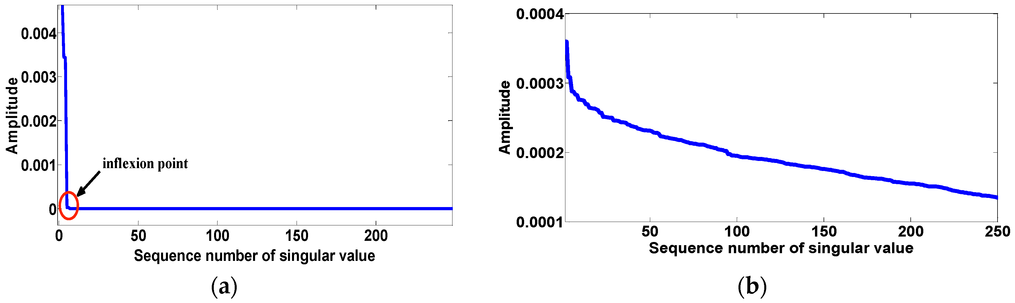
One can see from Figure 1a that the waveform of incremental singular entropy about the pure signal has an inflexion point on both sides of the curve which shows different tendencies. By contrast, there is no such point in this sequence in Figure 1b. Therefore, such an inflexion point can be used to identify those singular values that belong to the useful signal. Next, this paper chooses different methods to capture this point.

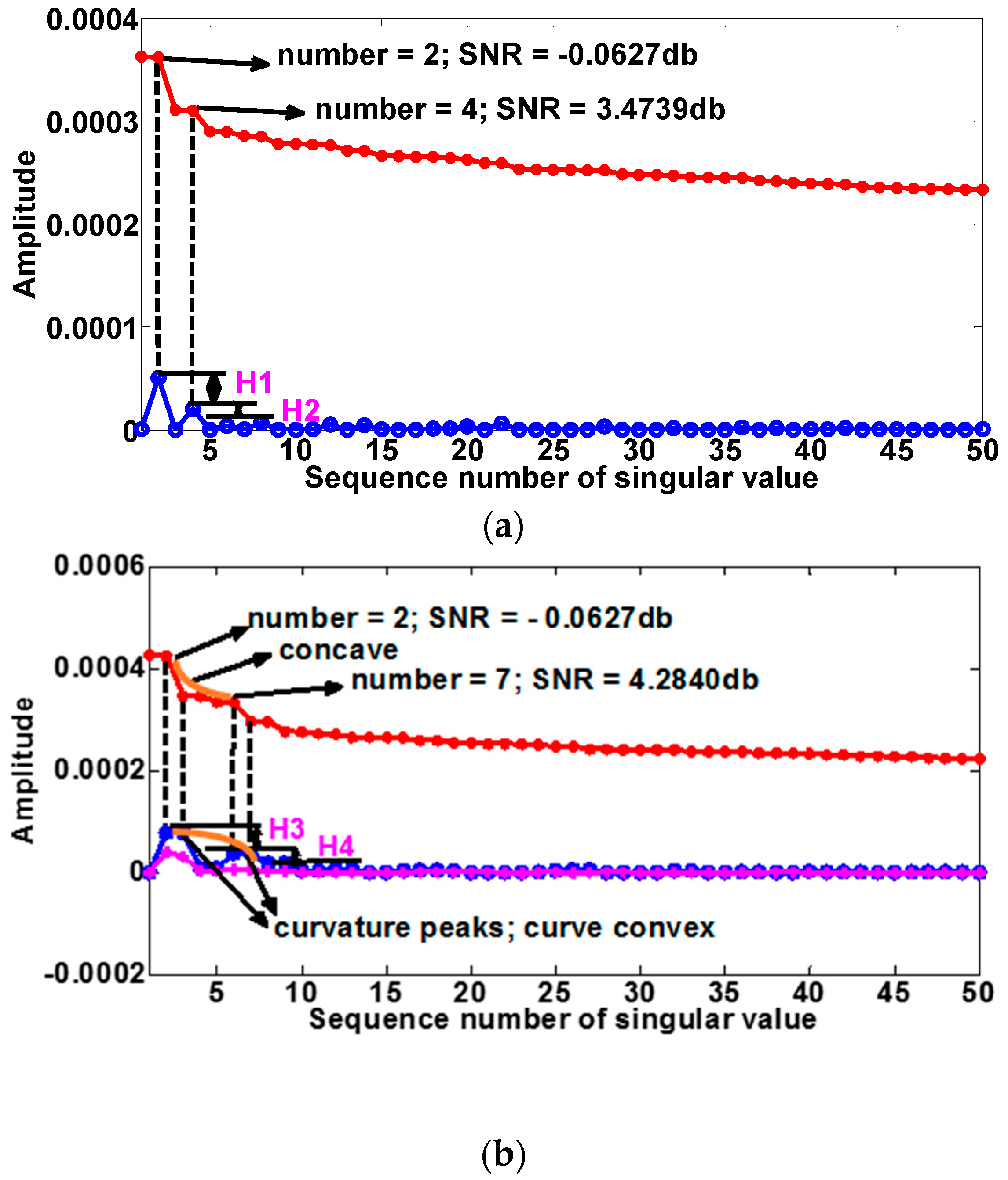
The red curve represents the spectrum of incremental singular entropy. A change of status occurs to the curve in a certain number of singular values before which the red curve has an interrupted decline, as shown in Figure 2a,b. The tendency becomes relatively flat as the number of singular values grows. However, determining the precise position of the turning point based on the incremental spectrum of singular entropy is difficult. Thus, a different spectrum of incremental singular entropy is introduced to identify the transformation of the curve. It can be seen from Figure 2a that some peaks are produced in the difference spectrum, which is represented by the blue curve, and that there is a maximum peak at the x-coordinate of 2. According to MPODSOISE, this paper chooses 2 as the number of effective singular values. However, the de-noised SNR is −0.0627 db, which is lower than the value of 3.4740, whose location happens to be the x-coordinate of the second maximum peak (x = 4). This means that some important components of the useful signal have been lost while choosing the effective number of singular values according to the maximal differential peak.

Next, the new method proposed by this paper is used to reflect the changing states of the spectrum. First, the blue curve represents the positive difference between two adjacent peaks. The gap H1 is larger than H2, which means that the second peak is the first one to have a large decline compared to the former peak. On the basis of MMBDSOISE, the second peak is regarded as the demarcation point for the selection of effective singular values that belong to the useful signal. Figure 2b shows the curvature spectrum of incremental singular entropy (blue line). For a clear display, two major peaks appear in the waveform, and their positions correspond to the location of inflexion of the singular spectrum (3 and 7).

Then, this paper uses the maximum peak of curvature to determine the effective number of useful signals based on the MPOCSOISE. The de-noised SNR is −0.0627 db (because the curve of the incremental singular entropy was concave at the position of the maximum peak, 2 is chosen as the final number of effective singular values). Finally MMBCSOISE was used to deal with this problem. The gap between the first two adjacent peaks, H3 is larger than H4, can be seen by the prominence of the pink curve. It is obvious that the second peak is the initial peak to have a larger decline compared to the former peak. As a result, the second peak could be viewed as the site of the demarcation point, and the number of effective singular values is 7 (because the curve of the curvature peak envelope (yellow curve) at 7 is convex) based on MMBCSOISE.

3.2. Noise Reduction Performance of the Simulation Signal

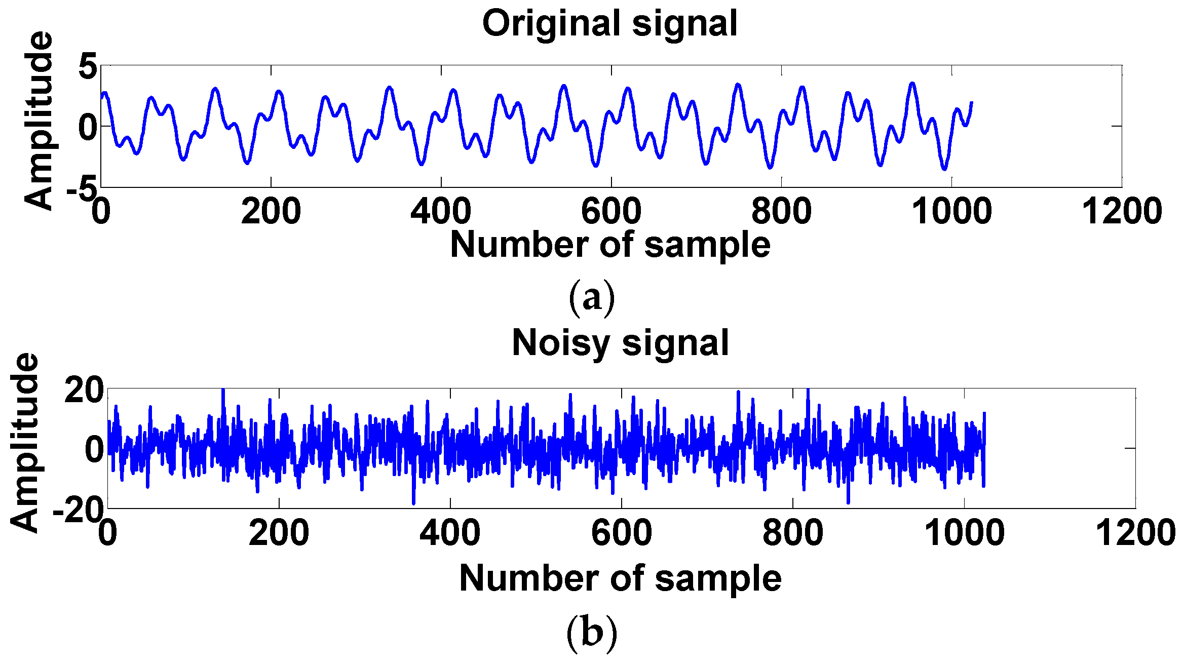
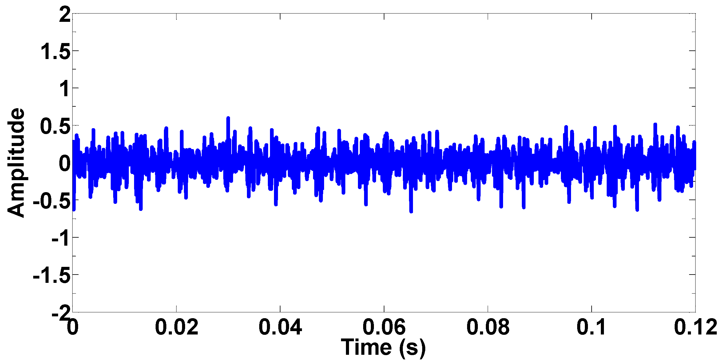
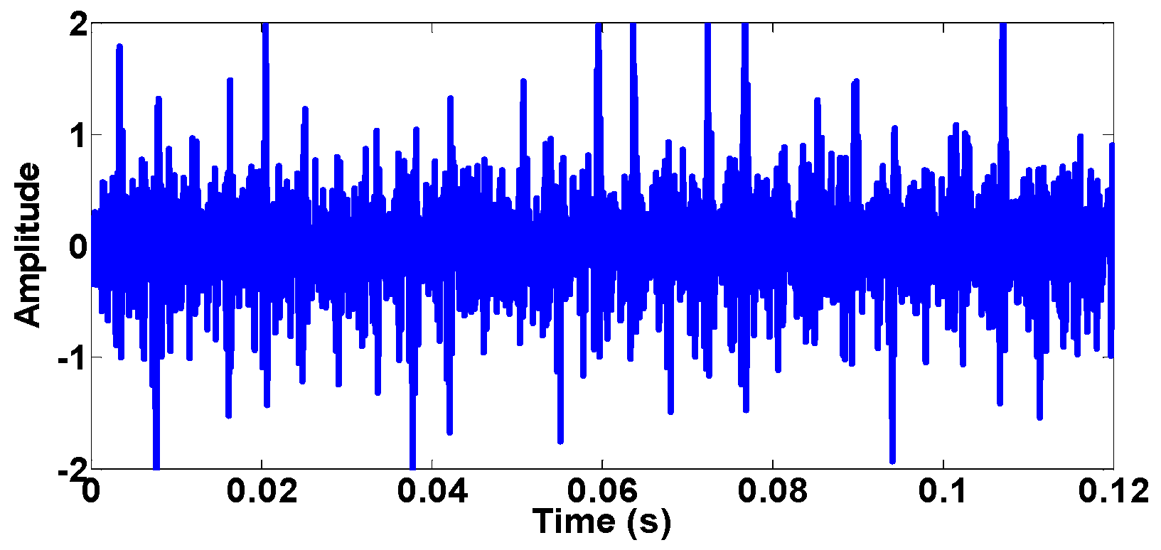
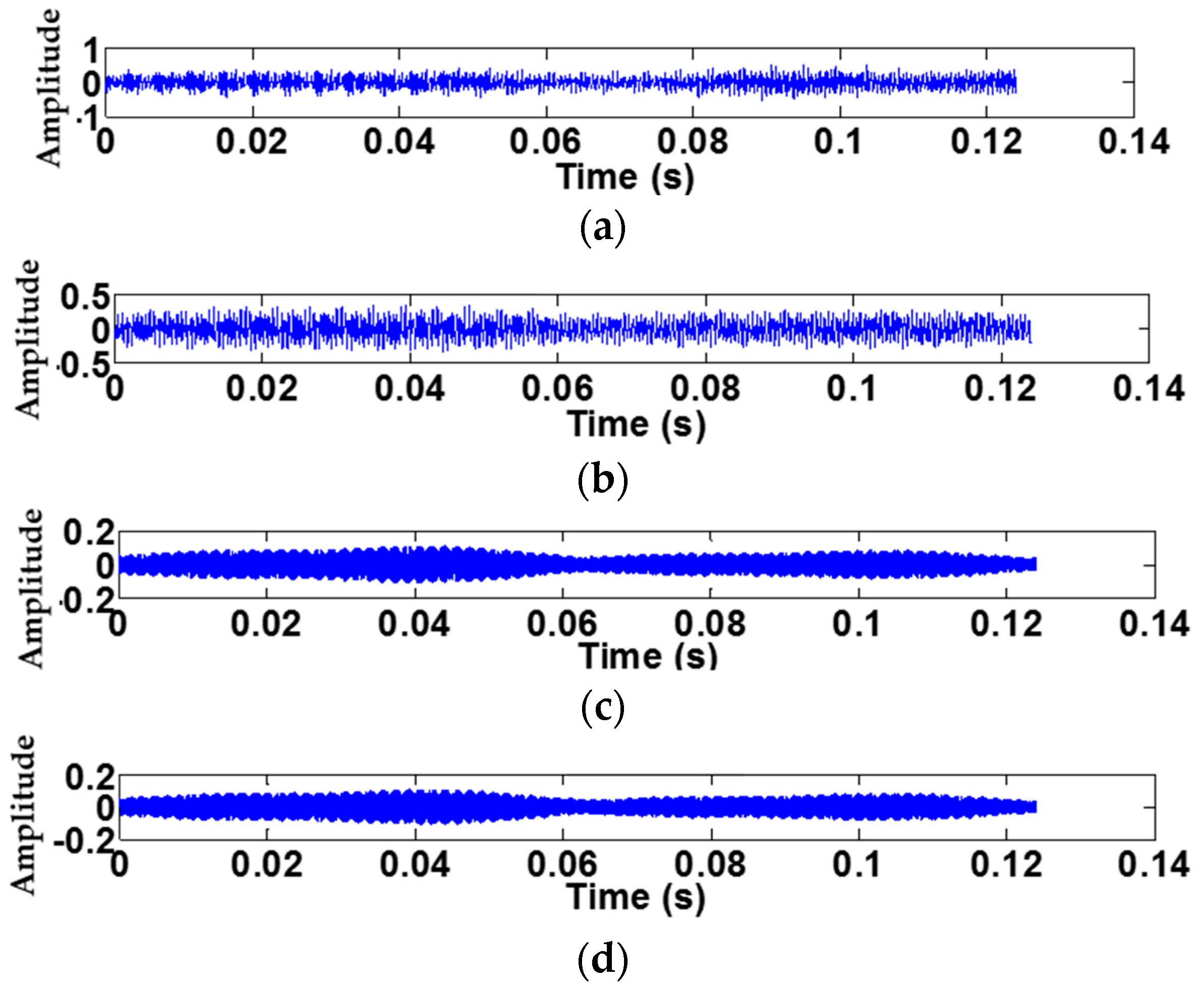
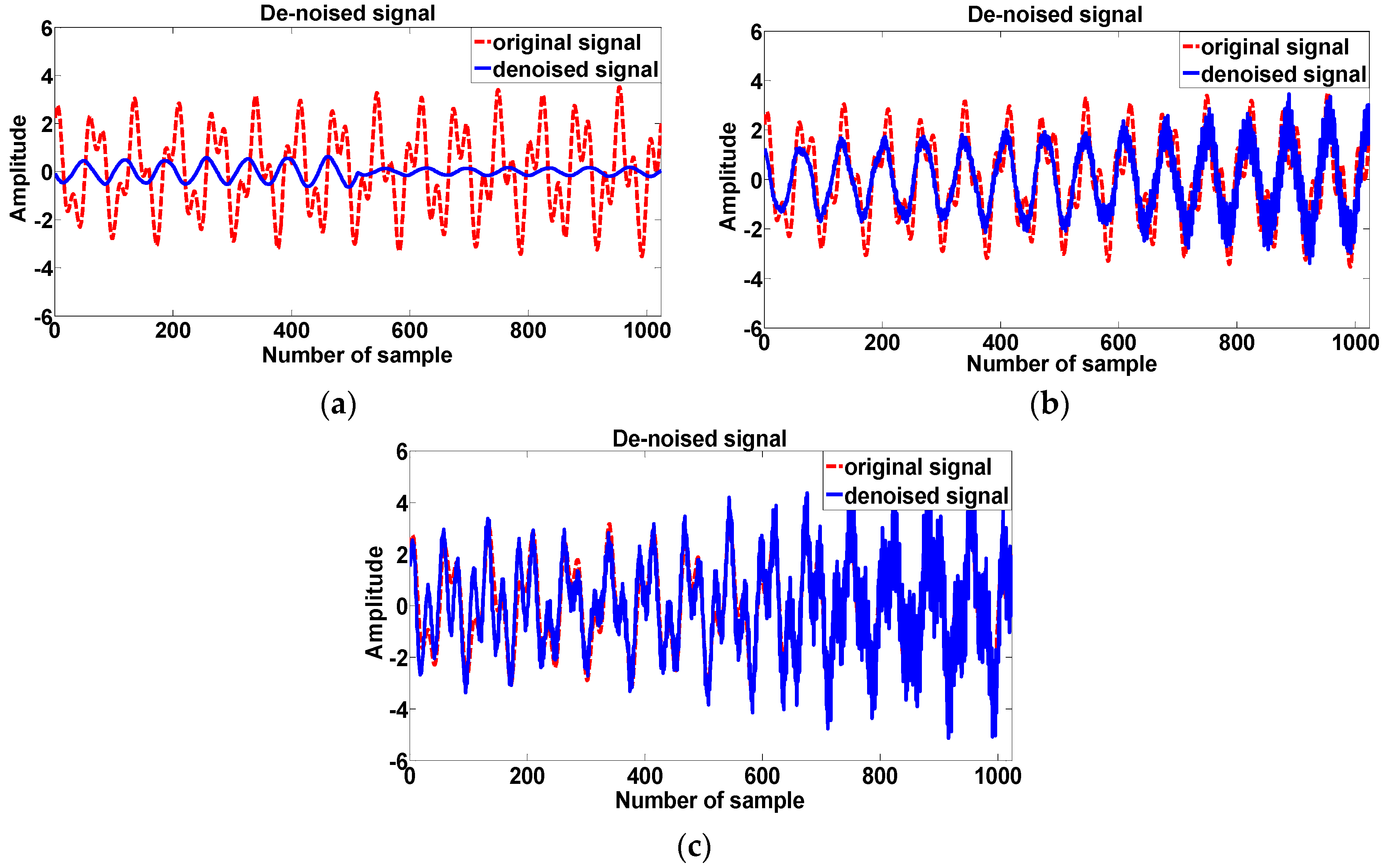
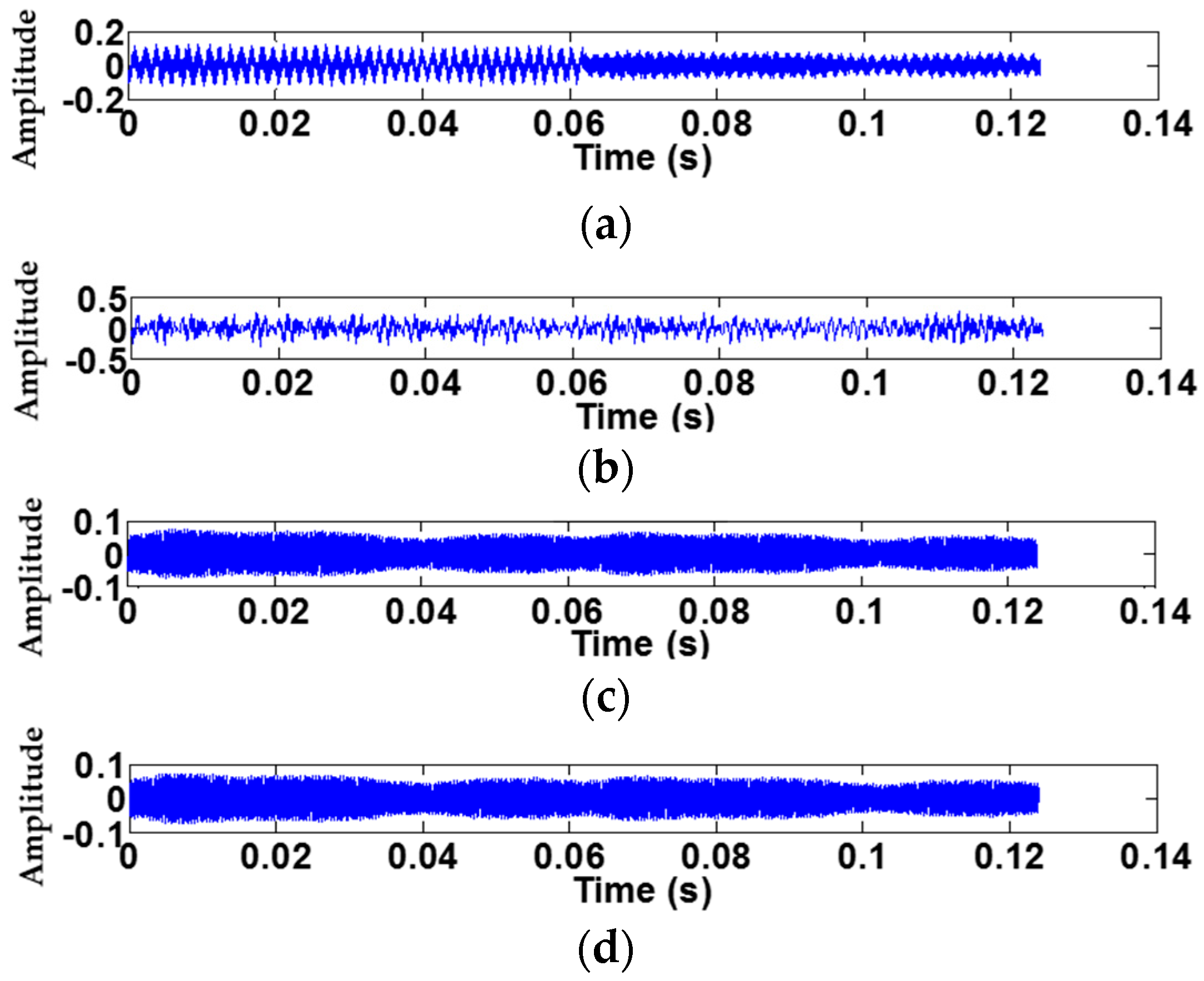
Figure 3b shows that the signal was submerged by the noise compared with Figure 3a. It is difficult to extract the main components of the useful signal. Figure 4 shows the effect of noise suppression based on three methods. First, the initial SNR of the noisy signal is −11.21 db; it can be seen in Figure 4a that the blue curve of the de-noised signal obviously deviates from the pure signal, and a waveform distortion has occurred in the whole time spectrum. This is because the effective order determined by MPODSOISE and MPOCSOISE is excessively small, which causes the loss of components of the original signal. By contrast, the coincidence of two curves in Figure 4b improves. Figure 4c shows that the de-noised signal curve fits the original signal better than the others; this is because the processing of de-noising based on MMBCSOISE takes the other major peaks, which contain significant information about useful signals, into account (not only maximum peak), completing the components of the pure signal. The components of the original signal were the best preserved based on MMBCSOISE. Next, this paper compared four methods from the view of the frequency domain.

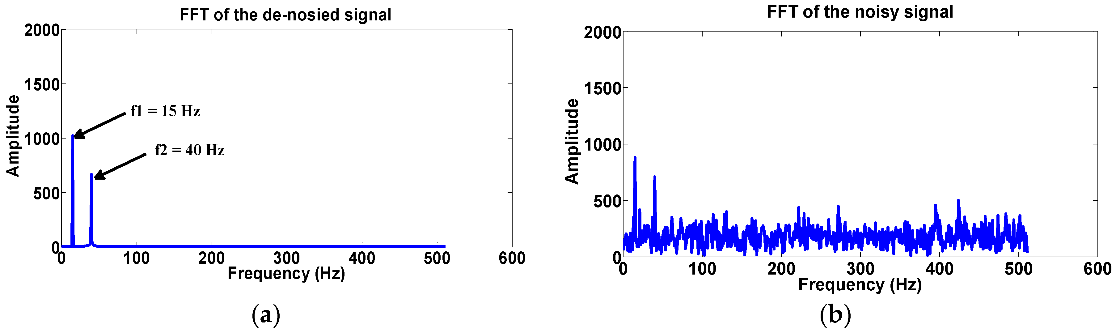
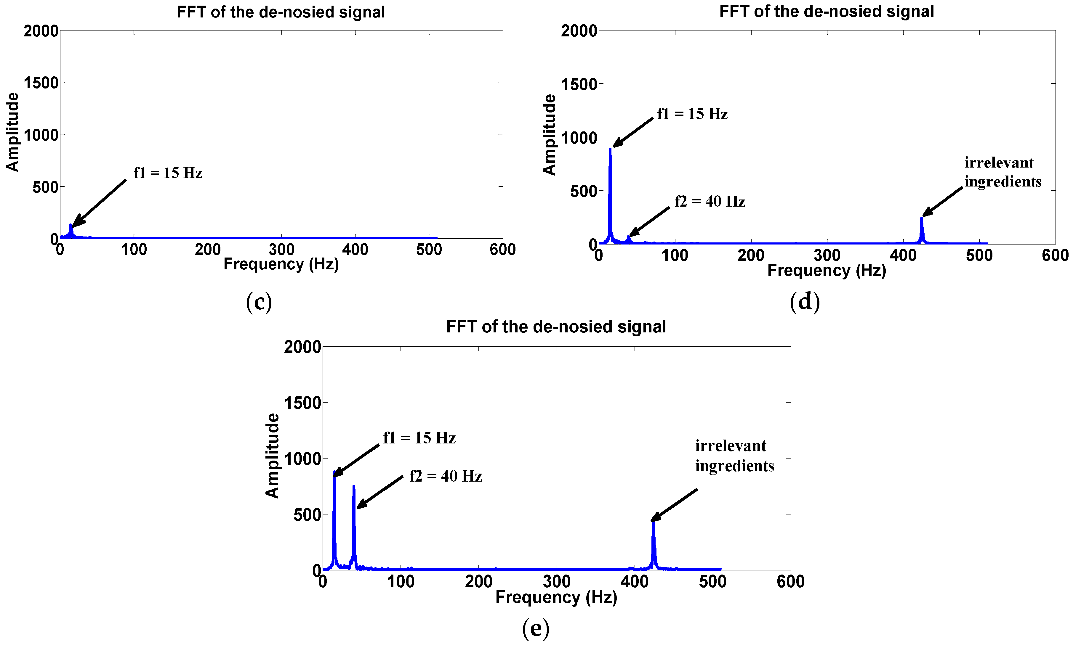
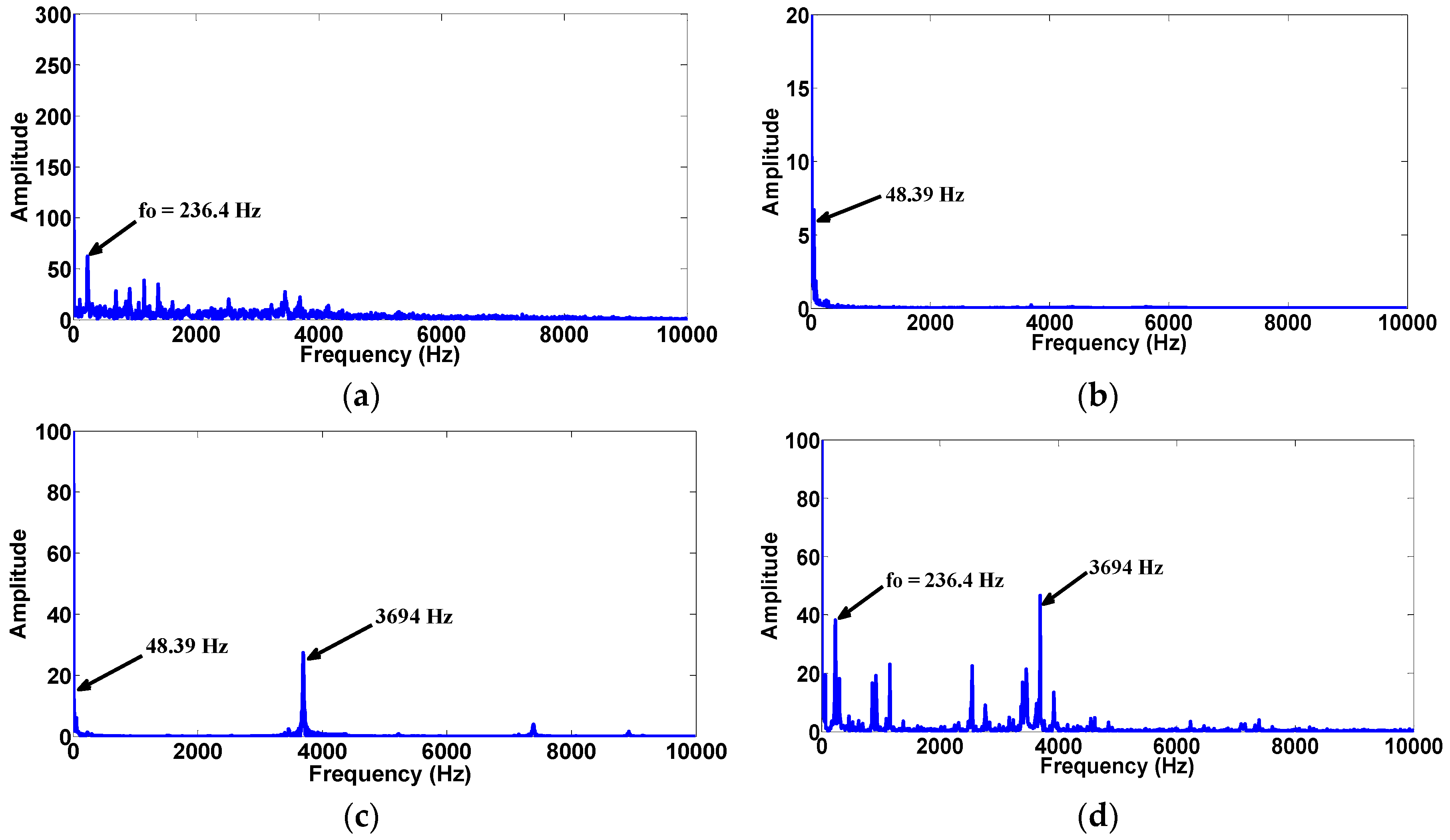
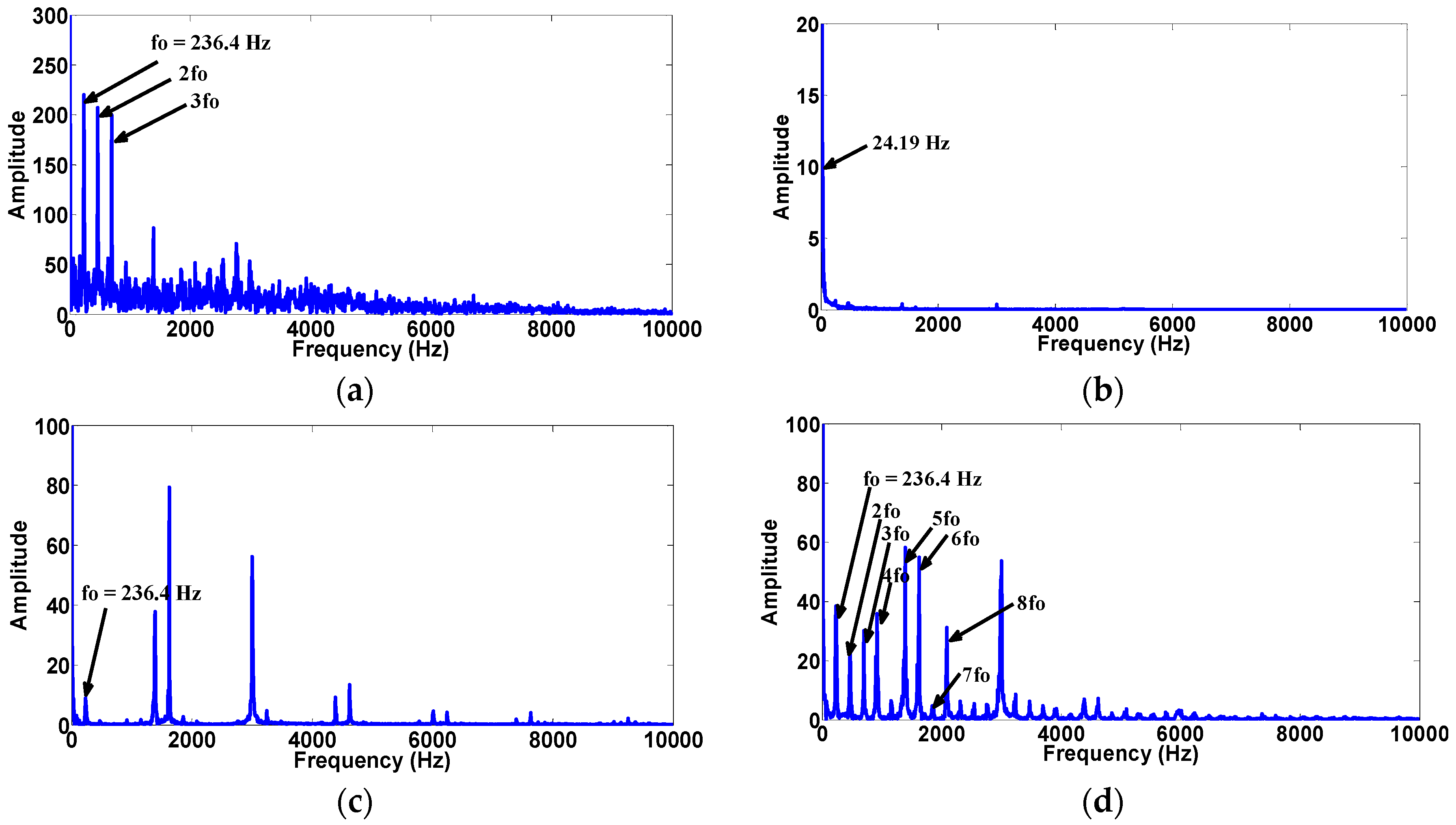
This paper conducts an FFT transform of the original and de-noised signals; Figure 5 reflects the corresponding frequency components. It is not difficult to extract the inherent frequencies of the original signal at 15 and 40 Hz in Figure 5a. Figure 5b is the frequency spectrum of the noisy signal, and the characteristic frequencies are submerged by the noise. Figure 5c–e are the de-noised frequency spectra, only the frequency component at 15 Hz appeared in Figure 5c and the signal component whose frequency is 40 Hz, are missing. Figure 5d recovers all of the frequencies; however, the amplitude of the 40 Hz frequency is smaller than the original spectrum. The frequency spectrum in Figure 5e is closest to the original signal. The characteristic frequencies of 15 and 40 Hz recovered although they introduced irrelevant ingredients, which also happened in Figure 5d, and it is for this reason that some residual noise is still preserved. What can be concluded from Figure 4 and Figure 5 is that the method presented in this paper retains the most useful signal components when de-noising, and the distortion caused by reconstruction was minimal.

3.3. Validation of Modified Method

To better evaluate the results of selecting effective singular values based on the four methods mentioned above, this paper conducted statistical analysis about SNR on the de-noised signal, depending on SVD. The number of effective singular values was determined by each method.

Table 1. Comparison of signal-to-noise ratio (SNR) and effective number of singular values about two de-noised signals.

Signal	Operation	MMBCSOICE	MPODSOISE	MPOCSOISE	MMBDSOICE
Signal one	Before de-noising	4.3483	4.3483	4.3483	4.3483
	After de-noising	24.1932	7.6607	7.6607	7.6607
	Number	5	4	4	4
	Before de-noising	−5.1941	−5.1941	−5.1941	−5.1941
	After de-noising	18.5129	6.5913	6.5913	6.5913
	Number	6	4	4	4
	Before de-noising	−11.2147	−11.2147	−11.2147	−11.2147
	After de-noising	4.2480	−0.0627	−0.0627	3.4739
	Number	7	2	2	4
Signal two	Before de-noising	3.4937	3.4937	3.4937	3.4937
	After de-noising	14.2194	6.0736	6.0736	6.0736
	Number	5	4	4	4
	Before de-noising	−2.5269	−2.5269	−2.5269	−2.5269
	After de-noising	13.1688	5.8545	5.8545	5.8545
	Number	5	4	4	4
	Before de-noising	−8.5475	−8.5475	−8.5475	−8.5475
	After de-noising	10.5862	4.7850	9.2128	4.7850
	Number	5	4	6	4

shows the results of noise reduction according to the four methods. The bold numbers signify the highest values of the de-noised SNR. The table shows that the effective numbers determined by MPODSOISE are minimal at all noise intensities. This is because MPODSOISE only considers the influence of the maximum peak of the difference spectrum of the singular value, which causes the loss of useful components. Then MPOCSOISE and MMBDSOICE followed. MMBCSOICE performs the task of noise reduction best among all of the methods, which could be seen from the most improved SNR in the first column. As a result, MMBCSOISE is better able to capture the demarcation point of the spectrum than other methods. The comparison results in the last column show that noise will be retained as the number of effective singular values is slightly larger. This may cause a decline in the de-noised SNR as well.

4. Experimental Verification

4.1. Experimental Installation of Bearing Faults

In order to verify the proposed method, this paper used data from the bearing run-to-failure tests on a specially designed test rig under normal load conditions. Four Rexnord ZA-2115 double-row bearings (REXNORD, Milwaukee, WI, USA) were installed on a shaft. The rotation speed was kept constant at 2000 rpm, while at the same time a radial load of 6000 lb was applied onto the shaft and bearing by a spring mechanism. All of the bearings were force lubricated, and their flow and temperature were regulated by an oil circulation system. Debris from the oil was collected by a magnetic plug installed in the oil feedback pipe in order to collect evidence of bearing degradation. The data sampling was 20 kHz and the data length was 20,480 [3].

Table 2. Corresponding parameters of the experimental bearings.

Bearing Designation	The Inner-Race Fault Frequency	The Outer-Race Fault Frequency	The Rolling Element Fault Frequency	The Fundamental Cage Frequency	The Ball Spin Frequency
ZA-2155 of Rexnord	fl (Hz)	fO (Hz)	fB (Hz)	fc (Hz)	fBS (Hz)
	296.9	236.4	139.9	14.8	70

gives the bearing characteristic frequencies for different faults and the corresponding parameters of the experimental bearing, including the outer-race fault frequency, f_O; the inner-race fault frequency, f_l; the rolling element fault frequency, f_B; the fundamental cage frequency, f_C; and the ball spin frequency, f_BS. These frequencies can be calculated according to the corresponding formula [3].

4.2. Analysis Result of the Outer Race Fault Signal

The acquisition time from 12 February 2004 10:32:39 to 19 February 2004 06:22:39 was for the performance degradation of outer race faults in bearing 1. Literature [3] gives the root mean square (RMS) value for the entire life cycle, which indicates the change of the bearings in the different periods of performance. The whole life cycle can be divided into three parts. At first, bearing operation keeps steady at the 0th–4th days (see phase I). Then the RMS increases to a certain level at the 5th day (see phase II). Some fluctuations appear in the temporal interval of the 5th and 6th days. Finally, a sharp rise occurs after half of the 6th day (see phase III). The changing trend of RMS over time illustrates the intrinsic characteristics of the damage propagating process: small spalls or cracks are formed and later smoothed by the continuous rolling contact in the failure of the initial state. When the damage spreads over a wider area, the vibration level rises again [5]. This paper extracted the data on the damage of the outer race in bearing 1 which chose 19 February 2004 00:42 as the occurrence of the early failure time. Next, 2480 samples were collected and time and frequency analysis was conducted.

First of all, we depicted the Time-domain waveform of the early out race fault in bearing 1 in Figure 6, what we can see from the figure that the failure signal is submerged by the noise and the waveform is so confused that it is impossible to extract the tiny components of the early fault signal. Figure 7 demonstrated the de-noised result based on four methods. It is obvious that the de-noised signal in Figure 7b is cleaner than others, and the vibration of the fault signal has been recovered. The second is Figure 7a, whose noise removal is not complete, although the vibration of the fault signal is embodied especially at 0–0.06 s. The waveforms in Figure 7c and Figure 7d have obvious differences compared with the former two and fail to reflect the oscillation of the fault signal. For the better identification of the de-noised signal, the reconstructed signals are demodulated with the Hilbert transform, and the envelope spectrum at each band is obtained.

It can be seen from Table 2 that the characteristic frequency of the outer race fault f_O is 236.4 Hz. Figure 8a shows that the whole envelope spectrum is covered by the noise in the early outer race fault, and the characteristic frequency is labeled “out”. As a comparison of the rest of the figures, characteristic components of faulty signals are lost in Figure 8b,c. In addition, there is an irrelevant component whose frequency is 48.39 Hz in Figure 8b, as well as 48.38 and 3964 Hz in Figure 8c. However, these frequencies are not inherent but are due to the periodic defects of bearings in the process of production [25], and this will cause the low reliability of the fault diagnosis resulting from these disturbances. All of the characteristic frequencies are reconstructed in Figure 8d, although some other invalid components have been introduced. It can be inferred that the effectiveness of the de-noised signal based on MMBCSOICE is better than others.

It can be seen in Figure 9 that the apparent transient impacts arose in the spectrum because of the serious outer race defect, which was buried by strong noise. Figure 10 exhibited the time domain spectrum of the de-noised signal based on different methods. The vibration of the fault signal is reconstructed integrally, and the transient signal can be obtained through applying the proposed method in Figure 10b. Nevertheless, the transient signals extracted by other methods such as MPOCSOISE and MPODSOISE still have strong noise. Figure 11 shows the filtered signal and its envelope spectrum. Mechanical equipment with gears and rolling bearing faults generally has a periodic pulse impact and exhibits the phenomenon of modulation of the vibration signal, which shows a uniform spacing modulating sideband of the meshing frequency or natural frequencies in the spectrum. In the first picture Figure 11a, the spectrum is so polluted by the noise that this paper can only find the characteristic frequency, f_O, and its two harmonics (e.g., f_O, 2f_O, 3f_O). The most harmonics preserved in the envelope spectrum of the de-noised signal are in Figure 11d. It can be seen from the spectrum characteristic frequency that six harmonics are restored (e.g., f_O–7f_O). On the contrary, the component of characteristic frequency was not recovered by MPODSOISE and MPOCSOISE in Figure 11b, and only the characteristic frequency f_O can be found in the envelope spectrum in Figure 11c.

In the process of extracting bearing outer race faults based on SVD, MMBCSOICE succeeded in locating the position of demarcation at which the singular value of the useful signal and the noise became separated. It is known from the experimental analysis that the number of effective singular values used to be small based on MPODSOISE and MPOCSOISE, which may cause the loss of important information about useful signals. It can be seen from Figure 8 and Figure 11 that there is no characteristic frequency in the envelope spectrum. Fortunately, this kind of situation improves based on MMBDSOICE and MMBCSOICE. Especially in the envelop spectrum obtained by MMBCSOICE presented in Figure 11d, even the higher-order harmonics (e.g., 6f_O, 7f_O) are evident. It can be concluded that the proposed MMBCSOICE is more effective at suppressing noise and extracting bearing fault characteristics, which increases the reliability and veracity in later incipient outer race defect detection.

5. Conclusions

Because early bearing faults are masked by signal noise, they are difficult to detect. Noise reduction is necessary for successful early bearing fault detection. The traditional methods of eliminating noise require prior knowledge of the signal and a lot of parameters to be set, meanwhile, a complicated iteration in the process of optimization may cause a decrease in real-time fault detection. Noise reduction based on dimensional reduction, such as SVD, is a better strategy for discovering the principle components of the useful signal.

The key to successful separation of noise and useful signal based on SVD is to choose the effective singular value that represents the useful signal, which can be used to reconstruct the de-noised signal. Seeking the effective singular value based on a traditional method such as maximum peaks of difference or the curvature spectrum often causes the distortion of the reconstructed signal, because the number of effective singular values determined by these older methods is small, which causes the loss of some information.

This paper uses the variation of difference of curvature peaks to accurately find the mutational site of the spectrum of incremental singular entropy, which is regarded as the number of effective singular values for SVD. The experiment results for dealing with real bearing data shows that the proposed method successfully extracted fault signatures under industrial noise and solved the problem of reduction of excessive noise caused by an unappropriated selected number of singular values. The results verified that SVD is a powerful tool that can offer available fault information for the later rolling element bearing fault diagnosis. However, this paper only discusses the circumstances of Gaussian white noise. In the next step, extracting the faulty signal under other noises such as color noise will be focused on to increase the reliability and universality of our method.