Opto-Acoustic Method for the Characterization of Thin-Film Adhesion

Abstract

The elastic property of the film-substrate interface of thin-film systems is characterized with an opto-acoustic method. The thin-film specimens are oscillated with an acoustic transducer at audible frequencies, and the resultant harmonic response of the film surface is analyzed with optical interferometry. Polystyrene, Ti, Ti-Au and Ti-Pt films coated on the same silicon substrate are tested. For each film material, a pair of specimens is prepared; one is coated on a silicon substrate after the surface is treated with plasma bombardment, and the other is coated on an identical silicon substrate without a treatment. Experiments indicate that both the surface-treated and untreated specimens of all film materials have resonance in the audible frequency range tested. The elastic constant of the interface corresponding to the observed resonance is found to be orders of magnitude lower than that of the film or substrate material. Observations of these resonance-like behaviors and the associated stiffness of the interface are discussed.

1. Introduction

Thin-film coating is used in a wide variety of applications ranging from micro-electro-mechanical systems (MEMS) to surface treatment of mechanical systems for wear-resistance enhancement. The recent trend indicates that reduced film thickness in a number of applications leads to better performance. In some cases, films of a few tens of nanometers in thickness are exposed to vigorous rubbing motion. With this trend, the quality control of the film-adhesion strength and endurance has become more important than ever. The reduction in the film thickness often means that a minute defect or imperfection at the film-substrate interface can cause significant coating damage, ending the life of the entire system.

A number of destructive and nondestructive methods have been developed to characterize the film-substrate adhesion. Those classified as destructive methods [1,2,3,4] assess the ultimate strength of the adhesion via measurement of the critical force that the coating can tolerate. Prevailing techniques classified as nondestructive methods use ultrasonic waves to probe the film-substrate interface [5,6,7,8,9]. An acoustic signal from an ultrasonic transducer is transmitted through the interface for the detection of abnormalities, such as delamination or defects. By measuring the velocity of the acoustic wave, it is possible to characterize the elasticity of the the interface.

The destructive methods are useful for a number of applications. However, they are not suitable for the evaluation of the endurance or fatigue characteristics. It is rare that the surface of a thin-film system is subject to external force comparable to the ultimate stress. The coating is usually damaged by repetitive, low-level stresses.

Similarly, the ultrasonic methods have limitations in practicability as the acoustic frequency used by most methods is unrealistically higher than the frequency range that a thin-film system normally experiences. As will be elaborated in the next section, the film-substrate interface can respond harmonically when driven at certain frequency ranges. Harmonic systems break most easily by repetitive use at or near the natural (resonant) frequency. This is true for a macroscopic system, as represented by the famous collapse of the Tacoma Narrows Bridge, or a micro-, nano-scale system, as represented by the fracture of a cantilever in MEMS. It is important to evaluate the adhesion strength using probing frequencies within a frequency range that thin-film systems are subject to and to examine if the interface exhibits resonance-like behaviors. The use of a proper frequency is important for a good signal-to-noise ratio, as well. If the probing frequency is orders of magnitude higher than the resonant frequency, the diagnostic system has poor sensitivity. The reduction in film thickness raises the ultrasonic frequency even higher. It is possible that the diagnostic system overlooks the most important frequency range.

Considering the above issues, we have devised an opto-acoustic method to characterize the film-substrate interface in a range of audible frequencies. In this method, the specimen is oscillated with an acoustic transducer perpendicular to the film surface, and the resultant differential displacement of the film surface to the substrate is read out optically. By sweeping the driving frequency of the transducer, it is possible to explore for resonance-like behavior of the interface.

Using this method, we studied the effect of a pre-coating surface treatment. The treatment, known as the oxygen-plasma bombardment technique, is widely used for thin-film coating on silicon substrates. According to the theory, plasma bombardment knocks off hydro-carbons and thereby strengthens the chemical bonding between the film and substrate materials. Using various film materials coated on the same silicon substrate with and without the surface treatment, we conducted experiments under various conditions and collected a great amount of data. Consequently, we observed several pieces of evidence that indicate that the film-substrate interface has resonance in a frequency range of 2 kHz to 30 kHz. The resonance behaviors were observed both in the specimen with the surface treatment (the treated specimen) and those with no surface treatment (the untreated specimen).

Analysis of the observed harmonic response indicates that the resonance behavior possibly represents the membrane-mode-like oscillation of the film surface [10] associated with the adhesion weakening mechanism, known as blistering [11,12,13]. The results of this study indicate the usefulness of this opto-acoustic method for practical applications. As mentioned above, harmonic systems most easily break when disturbed near resonant frequency, and audible frequency is abundant in environmental disturbance.

In this paper, we describe the opto-acoustic method, present the experimental study on the effect of the surface treatment for the silicon-based thin-films and discuss the results of the experiments focusing on the resonance behaviors observed in both the untreated and treated specimens. Furthermore, a possible elastic mechanism behind the resonance-like behavior observed in the audible frequency is discussed.

2. Theory

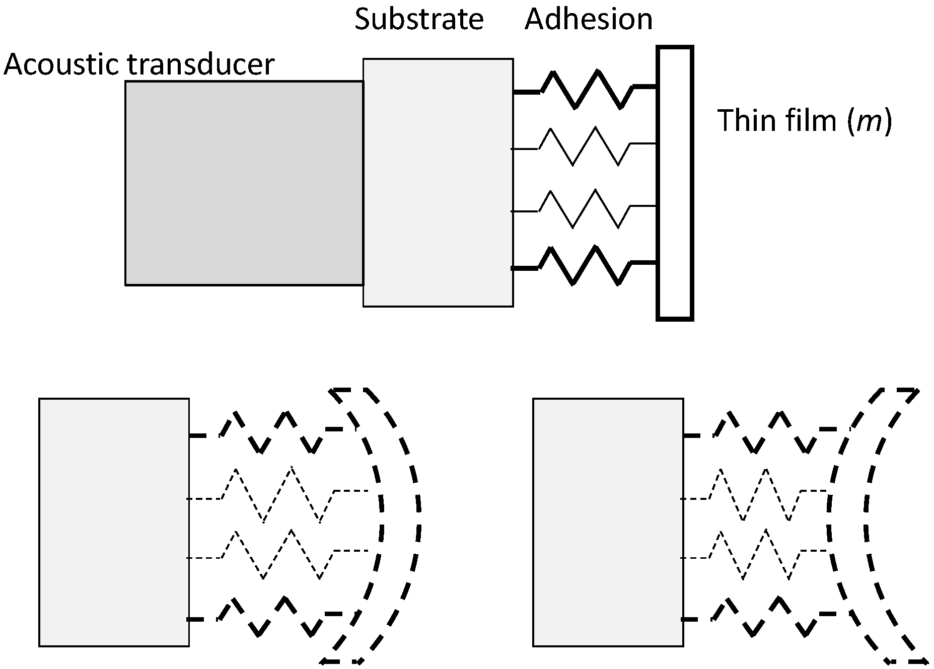
2.1. Elasticity of the Film-Substrate Interface

The main mechanism of film-substrate adhesion involves a collection of chemical bonds. Although the types and orientations of the chemical bonds are complex, each individual bond is associated with a certain elastic constant [14]. Thus, the film-substrate interface can be viewed as a complex combination of a number of springs, each having a different spring constant from one another. In an actual thin-film system, some of the bonds will not be perfect, leading to a lower elastic constant than the better bonds. Figure 1 illustrates the situation schematically where the middle two springs are weaker than the side springs. When this system is oscillated at a frequency lower than the resonance associated with some of the springs from the rear side of the substrate, the weaker springs oscillate more than the stronger springs. Consequently, the film surface can bulge back and forth as the film oscillates, as illustrated in the lower part of Figure 1. This type of membrane-like oscillation can occur locally in a specimen. By measuring the amplitude of the film surface oscillation scanning through the entire film surface, it is possible to characterize the elasticity of the film-substrate interface as a function of the position in the in-plane coordinates.

The ultrasonic technique known as scanning acoustic microscopy (SAM) probes the film-substrate interface by oscillating it at ultrasonic frequency. By measuring the acoustic velocity, SAM evaluates the elastic constant of the interface. Thus, SAM can potentially detect weak adhesions of thin-film systems. However, when the oscillation associated with adhesion weakness has a resonant frequency significantly lower than the ultrasonic frequency at which SAM is operated, the applicability of SAM becomes questionable for the following reason. When a thin-film system is driven acoustically, an oscillator whose resonance is the closest to the driving frequency responds most sensitively. The transmissibility (the transfer function) of a mechanical oscillator decreases with a quadratic dependence on the frequency ($f^{-2}$) on the high frequency side of the resonance. If the driving frequency is higher than the resonance, the response of the oscillator decreases quadratically. It is possible that bond imperfection reduces the overall stiffness so significantly that the ultrasonic frequency falls in a range where the sensitivity is unrealistically low.

2.2. Opto-Acoustic Method

In thin-film adhesion studies, the acoustical characterization of elastic behaviors associated with a resonant frequency lower than 100 MHz is difficult. The wavelength of the probing acoustic wave must be shorter than the width of the thickness of the film and substrate. To generate 10 or more wave numbers in a 100 $\mathsf{\mu }$m-thick silicon substrate, for instance, the wavelength must be shorter than 10 $\mathsf{\mu }$m. The acoustic velocity in silicon is approximately 8 km/s. Therefore, the corresponding frequency is of the order of 8 km/s ÷ 10 $\mathsf{\mu }$m = 800 MHz. For smaller thicknesses, the frequency must be increased further in proportion to the reduction in the wavelength. To overcome this difficulty, we use the opto-acoustic method described here.

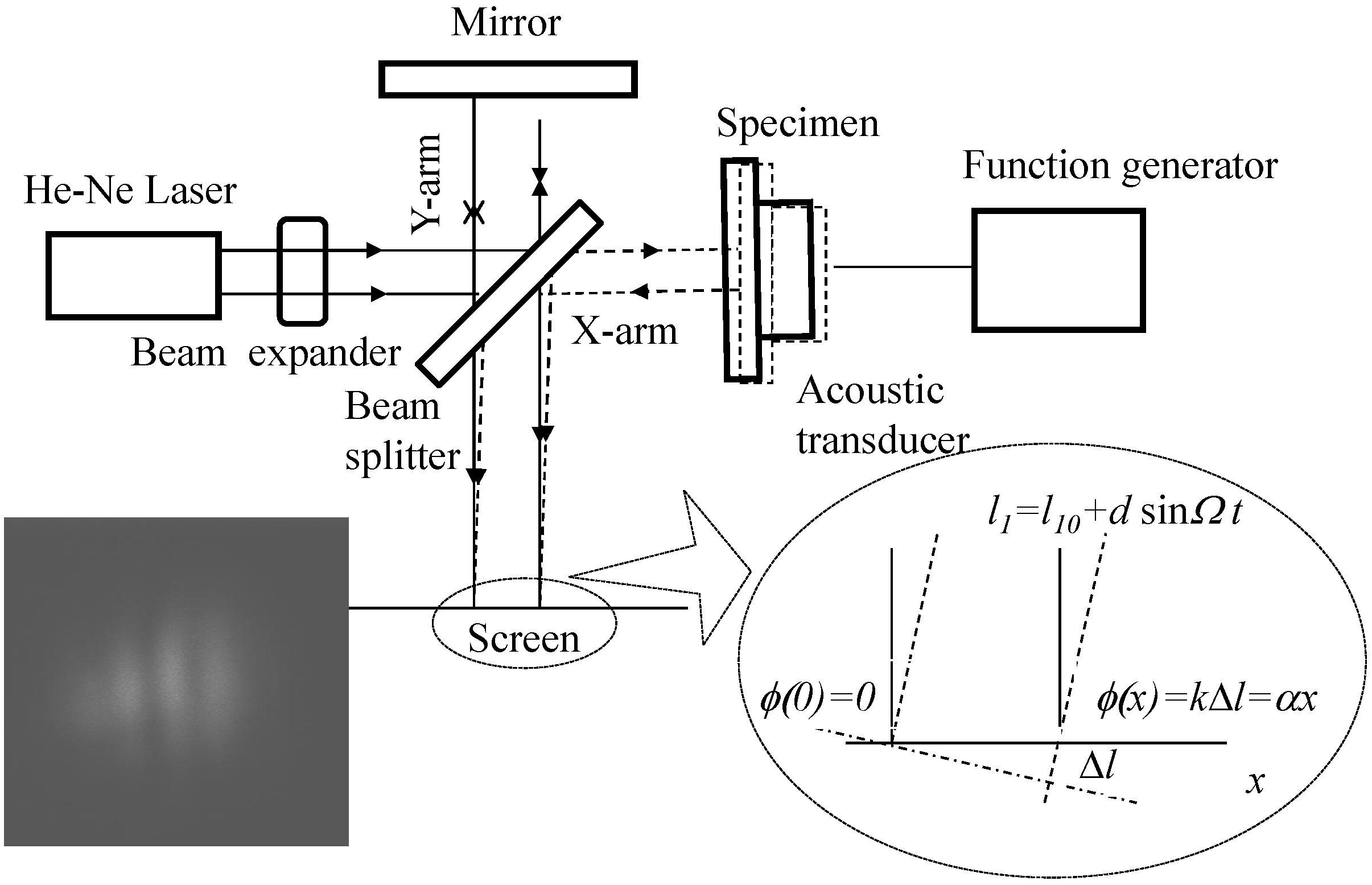
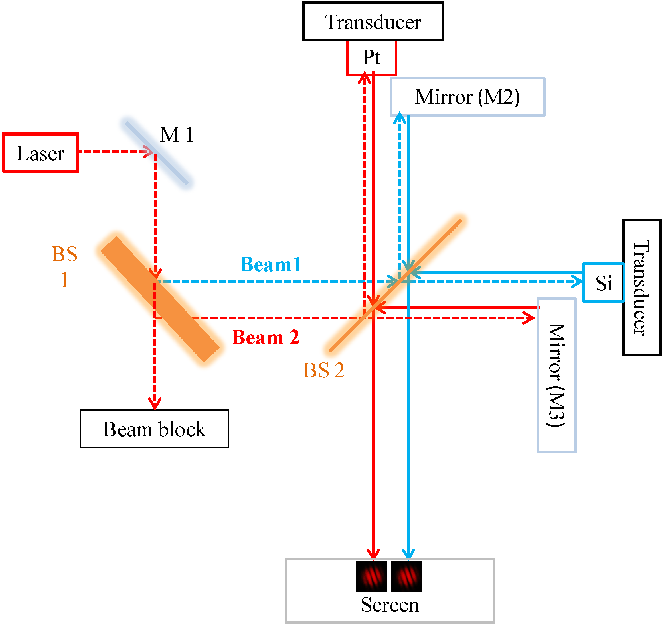
2.2.1 Michelson Interferometer

Figure 2 illustrates the optical configuration of this method. The specimen is integrated in a Michelson interferometer as one of the end-mirrors with the film side facing the beam splitter and is oscillated with an acoustic transducer from the rear. The acoustic transducer is driven with a sinusoidal input in a frequency range of 2 kHz to 30 kHz. The resultant oscillatory motion of the film surface is detected as the corresponding optical path difference behind the beam splitter.

To visualize the relative optical path length difference between the two arms, one of the end mirrors is slightly tilted. In this way, the relative phase of the optical intensity behind the beam splitter can be detected as parallel interferometric fringes as indicated by the insert in Figure 2. The fringe pattern is projected on a screen, and a digital camera is used to capture the pattern electronically. Here, the dark fringes represent the contour where the relative optical path length difference is totally destructive or the relative phase difference is an odd integer multiple of π. When the specimen is oscillated with the acoustic transducer, the corresponding optical path varies in a sinusoidal fashion, causing the dark fringes to dither around the nominal position where the dark fringes are located when the transducer is off. Since the digital camera’s frame rate is much lower than the transducer’s oscillation frequency, the dithering lowers the fringe contrast. The present method utilizes the reduction in the fringe contrast to estimate the oscillation amplitude.

In this frequency range, both the film and substrate behave as a rigid body because their elastic constants are so high that the acoustic phase velocities are high enough to make the wavelength at an audible frequency longer than their thicknesses. This means that if the interface has an elastic constant comparable to the film and substrate, the entire specimen should oscillate as a rigid body, as well. In other words, the oscillation amplitude of the rear and the front surface of the specimen is comparable or the transfer function of the rear-surface displacement to the front-surface displacement is unity. However, if the elastic constant of the interface is so low that the substrate-side to the film-side displacement transfer function is higher than unity, the film surface displacement becomes greater, as compared to the transducer’s displacement. The preliminary study on the harmonic response of a thin-film specimen demonstrated a case where the low elastic constant of the interface makes the substrate-to-film displacement transfer function greater than unity (see Section 3.1 below).

2.2.2. Principle of Operation

The reduction in the fringe contrast in a given image frame due to the dithering motion of the fringes can be argued quantitatively as follows. The optical intensity on the screen placed behind the beam splitter is given by the following expression.

$$I\left(t\right)=2I_0+2I_0\cos [k(l_{10}-l_{20})+kd\sin \omega t]$$

(1)

Here, $I_0$ is the intensity of the individual arm; k is the wave number of the laser beam; d is the amplitude of the film surface oscillation; and ω is the driving angular frequency provided by the transducer. Since one of the end-mirrors is tilted, the relative phase difference on the screen can be resolved as a linear function of x with a constant α as $k(l_{10}-l_{20})=\alpha x$. Here, the x-axis is set perpendicular to the dark fringes. Thus, Equation (1) can be rewritten in the following form.

$$I\left(t\right)=2I_0+2I_0[\cos \left(\alpha x\right)\cos \left(\delta \sin \omega t\right)-\sin \left(\alpha x\right)\sin \left(\delta \sin \omega t\right)]$$

(2)

where $\delta =kd$. Using Bessel functions of the first kind, Equation (2) can further be rewritten as follows.

$$I\left(t\right)=2I_0[1+\cos \left(\alpha x\right)\{J_0\left(\delta \right)+2J_2\left(\delta \right)\cos \left(2\omega t\right)+\cdots \}-\sin \left(\alpha x\right)\{2J_1\left(\delta \right)\sin \left(\omega t\right)+2J_3\sin \left(3\omega t\right)\cdots ]$$

(3)

Therefore, the signal of the digital camera is:

$$\begin{array}{ccc}\hfill S\left(\tau \right)& \propto & {\int }_0^{\tau }\{1+\cos \left(\alpha x\right)\left\{J_0\left(\delta \right)\right\}dt\hfill \\ \hfill & +& 2\cos \left(\alpha x\right)\sum _{m=1}^N{J}_{2m}\left(\delta \right){\int }_0^{\tau }\cos \left(2m\omega t\right)dt\hfill \\ & -& 2\sin \left(\alpha x\right)\sum _{m=1}^N{J}_{2m-1}\left(\delta \right){\int }_0^{\tau }\sin \left\{(2m-1)\omega t\right\}dt\hfill \end{array}$$

(4)

Since the frame rate of the digital camera is much lower than the driving frequency, the exposure time τ is much longer than the period of the film surface oscillation. Consequently, the values of the oscillatory terms in Equation (4) ${\int }_0^{\tau }\cos \left(2m\omega t\right)dt$ and ${\int }_0^{\tau }\sin \left\{(2m-1)\omega t\right\}dt$ sweep through a number of periods as t is varied from zero to τ in the integration. On the other hand, the values of the first two terms that do not contain an oscillatory term increase in proportion to τ. Therefore, the signal from the digital camera is dominated by the first non-oscillatory terms of Equation (4). Thus, the signal $S\left(\tau \right)$ can be approximately expressed as follows (The concept is similar to the technique known as the amplitude-fluctuation electronic speckle pattern interferometry (AF-ESPI) [15,16]. The difference is that AF-ESPI involves image subtraction from a reference image, and the present method extracts the oscillation amplitude from a given image frame of the interferometric fringe pattern without subtracting a reference image.):

$$S\left(\tau \right)\propto \tau +J_0\left(\delta \right)\cos \left(\alpha x\right)a\tau$$

(5)

Equation (5) indicates that the peak value of the spatial Fourier spectrum of $S\left(\tau \right)$ (the value of the peak at the lowest spatial frequency) is proportional to $J_0\left(\delta \right)$. When the film surface is still or the acoustic transducer is turned off, $d=0$, hence $\delta =0$. Since $J_0\left(0\right)=1$ and $J_0\left(\delta \right)$ monotonically decreases to zero in the range of $0<\delta <2.4$, the peak value of the Fourier spectrum decreases as the oscillation amplitude increases in the corresponding range. The Fourier spectrum peak value of a given signal obtained with the film surface oscillation amplitude can be evaluated relative to the still film surface case (called the relative peak value) as $J_0\left(\delta \right)/J_0\left(0\right)=J_0\left(\delta \right)$. By obtaining the relative peak value experimentally, i.e., by comparing the Fourier spectrum peak value of a given signal with that obtained with no film surface oscillation, it is possible to estimate $\delta =kd$ and, hence, d.

2.2.3. Proof of Principle

Figure 3 (1) shows examples [17,18] of fringe patterns and the Fourier spectrum of the intensity profile along a horizontal line around the vertical center. The left fringe pattern (a) is the case where the film was coated without a surface treatment; the middle (b) is where the film was coated after the silicon substrate was treated with the oxygen-plasma bombardment technique; and the right (c) is where the transducer was turned off. Careful observation will indicate that the fringe contrast increases from (a) to (c). The driving frequency was 11.5 kHz for all three cases. The observed fringe contrasts indicate that at this driving frequency, the surface treatment made the amplitude of the film-surface oscillation smaller than the untreated case. Naturally, the contrast is highest when the transducer was turned off.

The left plots shown under the fringe images, Figure 3 (2), are the Fourier spectra of the optical intensity profile along the horizontal line at the vertical center as indicated in the leftmost fringe image. The unit of the horizontal axis of the spectrum is the inverse of the pixel numbers. The left group of three plots whose first spectrum peaks appear approximately at the spatial frequency of 0.0125 1/pxl result from the three fringe images (a) to (c). The peak values of the three spectra indicate the fringe contrast quantitatively; the spectrum peak decreases as the fringe contrast decreases, being consistent with Equation (5).

The three plots shown on the right part of Figure 3 (2) are the Fourier spectra for the non-coated specimen (the bare silicon specimen) obtained in the same fashion as the left three plots. The three plots are the cases where the transducer oscillated one end-mirror only, oscillated the other end-mirror only and oscillated neither end-mirror, respectively (the use of the same plot marker as the left group indicates that the same mirror was oscillated). The peak values for the three cases are practically the same, indicating that the silicon surface oscillation amplitude was below the sensitivity of the interferometer.

In the frequency domain, the amplitude of the film-surface displacement is the product of the transfer functions of the layers between the transducer surface and the film surface and the Fourier transform of the transducer-surface displacement. The overall transfer function can be expressed as the product of the transfer functions of (a) the transducer surface to the rear surface of the silicon substrate, (b) the rear to the front surface of the silicon substrate, (c) the silicon to the film surface, (d) the rear to the front surface of the Ti film and (e) the transfer functions of the interface between the first and second metal layers (for the Ti-Au and Ti-Pt specimens only). Here: (a) is the transfer function of the glue (epoxy) used to bond the specimen to the transducer; (b) is the silicon substrate itself; (c) is the substrate-film interface; (d) is the film itself; and (e) is the product of the transfer functions of the metal-metal interface and the second metal film itself.

Of these transfer functions, those of the silicon substrate and the metal film itself are considered unity due to the high stiffness as mentioned above. The metal-metal interface in (e) is also considered unity, as it is metallic bonding. As for the epoxy, a theoretical estimation indicates that the resonant frequency of the epoxy is over 30 MHz under the present condition and thereby can be assumed unity in the frequency range used in this experiment. Thus, of (a) through (e), all of the transfer functions, except (c), are considered unity under the driving frequency ranging from 5 kHz to 30 kHz. After all, the harmonic response evaluated by the Fourier spectrum, like Figure 3 (2), represents the behavior of the substrate-film interface.

According to Equation (5), the peak value of a Fourier spectrum, like Figure 3 (2), is proportional to $J_0\left(\delta \right)=J_0\left(kd\right)$. To validate this proportionality, an additional experiment was conducted. In this experiment, we varied the oscillation amplitude of the transducer surface by changing the amplitude of the electric input and measured the peak value of the resultant Fourier spectrum. Here, since the square of the voltage is proportional to the electric power and the square of the oscillation amplitude is proportional to the mechanical power, the input voltage and the oscillation amplitude are proportional to each other. Figure 3 (3) plots the spectral peak value as a function of the input voltage to the transducer. The three plots are for the untreated and treated Ti-Au specimens and the bare silicon specimen. The driving frequency is 10.42 kHz. Also plotted in Figure 3 (3) is a theoretical curve computed for each specimen based on Equation (5). Since the transfer function from the amplitude of the input voltage to the amplitude of the film-surface displacement is unknown, the theoretical curve is adjusted in the form of $J_0\left(aV\right)$, where V is the input voltage and a is a fitting parameter used for each curve. Physically, the parameter a corresponds to the transfer function from the transducer voltage to the film-surface oscillation. Reasonable agreement is seen between the experiment and theory.

3. Experimental Section

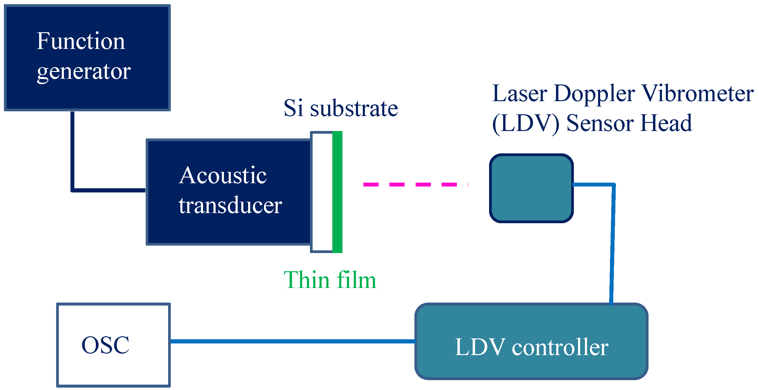
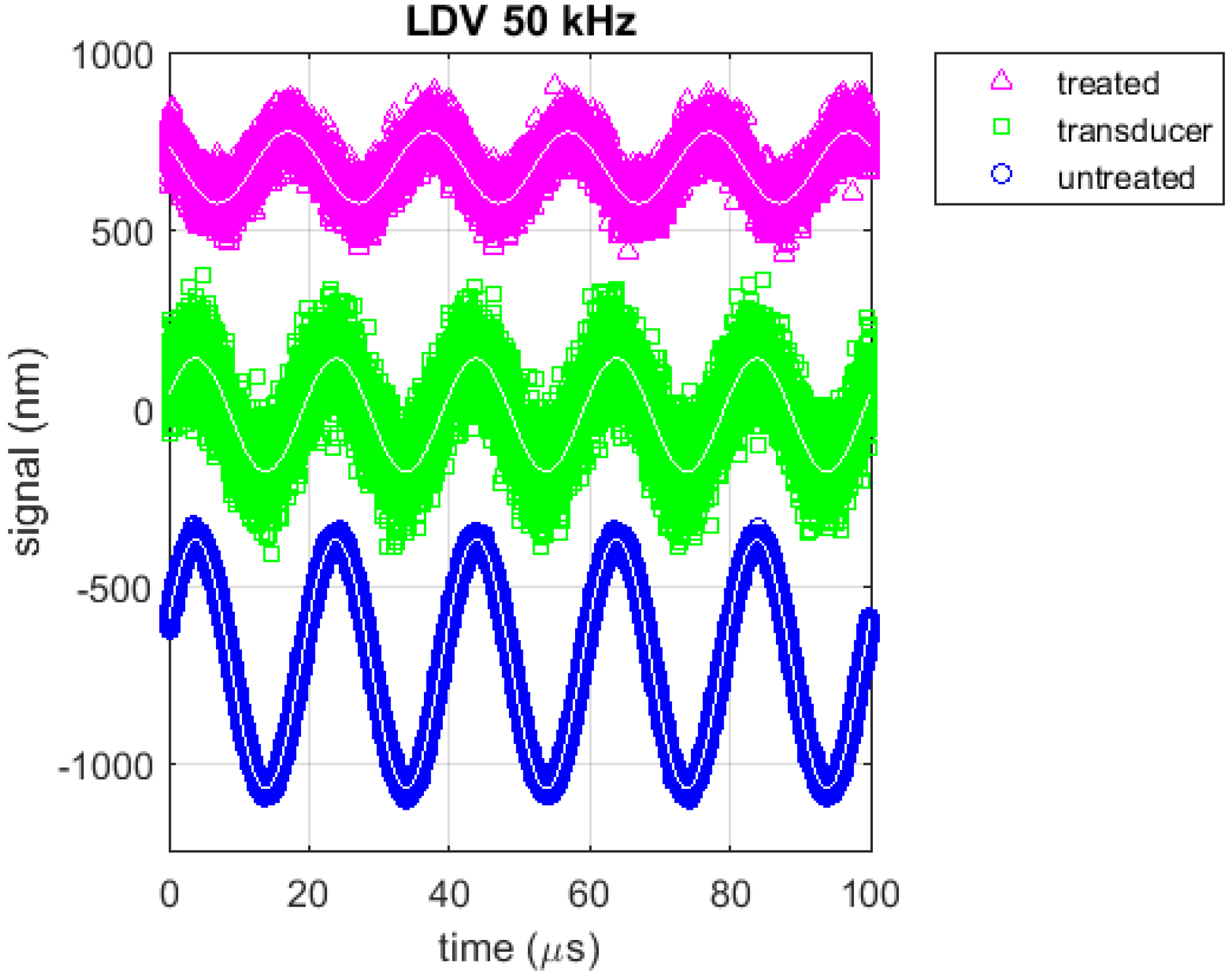
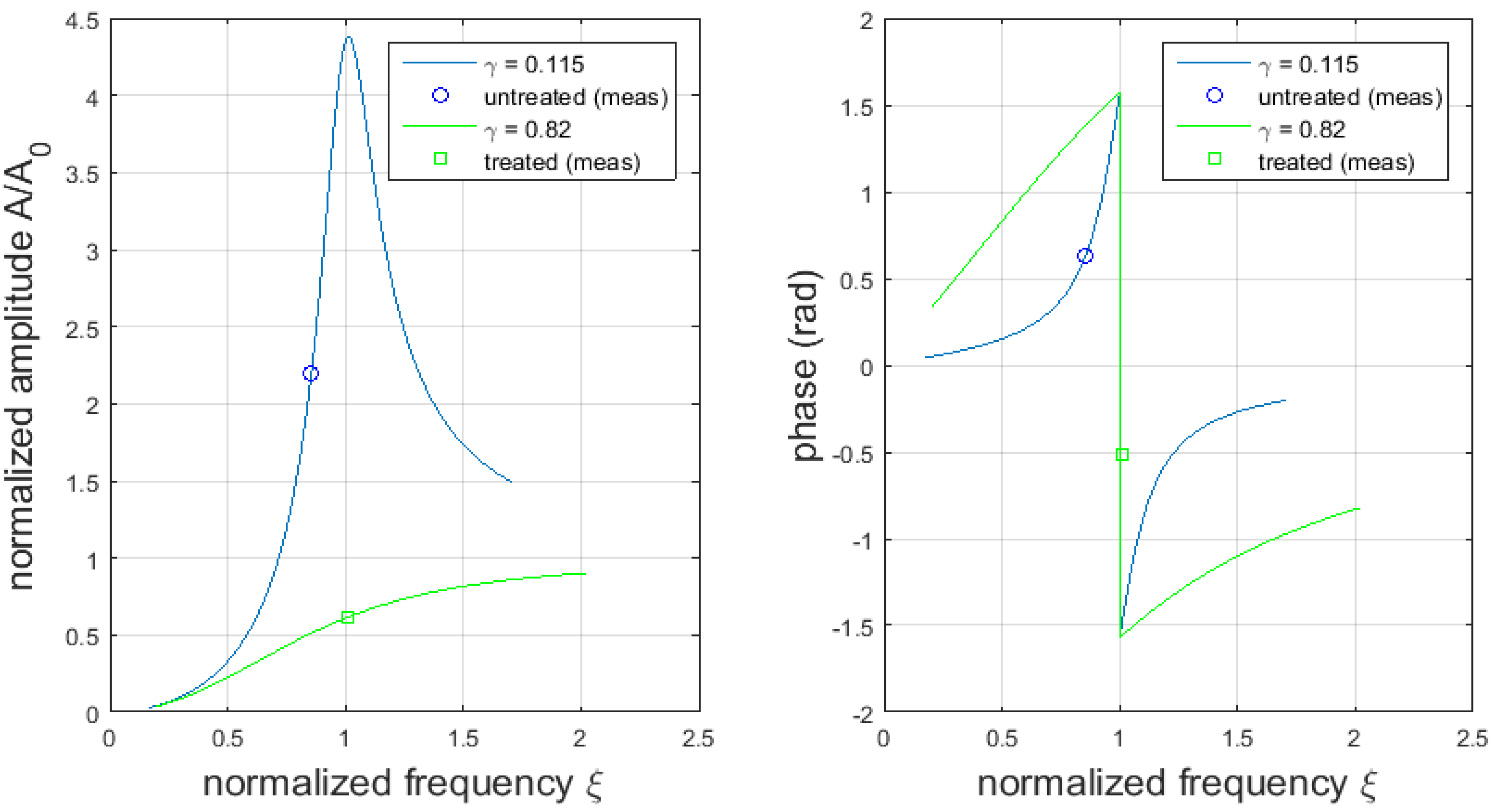
3.1. Preliminary Experiment with Doppler Vibrometry

We first studied the harmonic response of a thin-film specimen using a laser Doppler vibrometer (LDV, Model: OFV 5000, Polytec, Irvine, CA, USA [19] with Displacement Decoder Model: DD300, Polytec, Irvine, CA, USA [20]) [21]. Figure 4 illustrates the experimental arrangement. The operation principle of LDV can be found elsewhere [22]. In short, it works in the following fashion. A laser beam is applied normal to an oscillating surface. The sensor of the LDV compares the optical frequency of the reflected laser beam with the incident beam. Due to the Doppler effect, the frequency of the reflected beam is shifted depending on the velocity of the oscillation. From the detected frequency shift, the oscillation amplitude is estimated.

A pair of polystyrene thin-films were used in this experiment. In the first specimen, 100 nm-thick polystyrene was coated on a 750 $\mathsf{\mu }$m-thick silicon substrate without pre-coating surface treatment (untreated polystyrene-coated specimen). The silicon substrate was cut along the [1, 0, 0] plane. In the second specimen, polystyrene of the same thickness was coated on the same silicon substrate after the surface was treated with the oxygen-plasma bombardment technique.

An acoustic transducer was attached to the rear surface of the specimen to oscillate it at 50 kHz. The transducer was driven with a function generator (Model 395, Wavetek, San Diego, CA, USA) with a pure sinusoidal output. Figure 5 compares the resultant displacement of the film surface for the untreated and treated specimens along with the oscillation of the transducer surface. (The signals for the untreated and treated specimens are shifted vertically for better visibility. The amplitude of the signals in nm exceeds the maximum value specified by the manufacturer for an unknown reason. However, since the signals do not exhibit any saturation-like behavior, the argument made here is considered legitimate. The absolute amplitude of the oscillation does not affect the gist of the argument.) Here, the middle graph is for the case when the transducer was oscillated without a specimen; the top and bottom graphs are the cases where the treated and untreated specimens were attached, respectively. The top and bottom graphs are shifted vertically for better visibility. As expected, the untreated specimen shows greater oscillation amplitude, indicating that the adhesion is weaker. (Figure 5 indicates that the signal from the treated specimen and the transducer only is much noisier than the signal from the untreated specimen. The reason for this observation is not totally clear. A possible explanation is that: (a) the untreated one is least noisy because the amplitude of the signal is the greatest (among the three signals); (b) the amplitude of the transducer-only signal is not much smaller than the untreated, but the signal is much noisier than the untreated case because the surface of the transducer was not as smooth as the specimen; (c) the treated signal is noisy because the signal was low.) There is a phase difference between the untreated and treated specimens, as will be discussed shortly.

Consider the film surface motion based on the theory of harmonic oscillation. The harmonic response of an oscillatory system of spring constant k, damping coefficient b and mass m driven at angular frequency ω is given as a solution to the following equation of motion.

$$m\ddot{x}+b\dot{x}+kx=f{e}^{i\omega t}$$

(6)

Here, $x\left(t\right)$ is the displacement from the equilibrium position of m, and f is the amplitude of the driving force. In the present context, k and b represent the elasticity and viscosity of the adhesion; m is the mass of the thin-film; and ω is the angular frequency of the acoustic transducer. The particular solution to Equation (6) can be put in the following form in general.

$$x\left(t\right)=A{e}^{i(\omega t-\delta )}$$

(7)

Substitution of Equation (7) into Equation (6) leads to the following condition regarding the amplitude and phase of the oscillation of the film displacement:

$$\begin{array}{ccc}\hfill A& =& \frac{f/m}{\sqrt{{({\omega }_0^2-{\omega }^2)}^2+4{\beta }^2{\omega }^2}}\hfill \end{array}$$

(8)

$$\begin{array}{ccc}\hfill \tan \delta & =& \frac{2\beta \omega }{({\omega }_0^2-{\omega }^2)}\hfill \end{array}$$

(9)

Here, ${\omega }_0=\sqrt{k/m}$ is the natural frequency of the oscillatory system, and $2\beta =b/m$. $f/m$ in Equation (8) is the acceleration of the transducer surface. The amplitude of the transducer surface $A_0$ when the transducer is operated at ω can be related to the acceleration as $(f/m)=A_0{\omega }^2$. Using this relation, we can rewrite Equations (8) and (9) in the following forms.

$$\begin{array}{ccc}\hfill \frac{A}{A_0}& =& \frac{{\xi }^2}{\sqrt{{(1-{\xi }^2)}^2+4{\gamma }^2{\xi }^2}}\hfill \end{array}$$

(10)

$$\begin{array}{ccc}\hfill \tan \delta & =& -\frac{2\gamma \xi }{(1-{\xi }^2)}\hfill \end{array}$$

(11)

where the frequency and damping coefficient are normalized by the natural frequency as $\xi =\omega /{\omega }_0$ and $\gamma =\beta /{\omega }_0$.

Since the left-hand sides of Equations (10) and (11) can be experimentally determined from Figure 5, we can estimate the natural frequency and decay constant for a given driving frequency by finding the combination of ${\omega }_0$ and γ that yields $A/A_0$ and $\tan \delta$ closest to the experimental values. Figure 6 plots theoretical $A/A_0$ and $\tan \delta$ as a function of ξ (solid lines) and the experimental values determined from Figure 5 (square and circle markers) for the driving frequency of 50 kHz. For the untreated/treated specimen, when ${\omega }_0$ and γ are as shown in

Table 1. Amplitude and phase of the Doppler vibrometry signal relative to transducer and corresponding natural frequency and decay constant estimated from Equations (10) and (11).

Specimen	Untreated	Treated
$A/A_0$	2.2	0.62
δ (rad)	1.63	−0.52
${\omega }_0/2\pi$ (kHz)	58.5	49.5
γ (1/s)	0.115	0.82

, the experimental values agree with the theory the best. It is seen that the untreated specimen shows 18% higher resonant frequency than the treated specimen and that the surface treatment makes the elastic dynamics more energy dissipative. This 18% ratio of the resonant frequency of the untreated specimen to the treated specimen observed in the polystyrene films is approximately the same as the case of the other films tested in the study (see Section 3.2 below for more details). This agreement can be simply a coincidence, but is interesting to note. The higher energy dissipation in the treated specimen can be understood by considering that the oxygen plasma bombardment makes the substrate surface rougher and causes more friction when the layers undergo oscillatory motions.

3.2. Analysis on Ti-Si Thin-Film Specimens with the Acousto-Optical Method

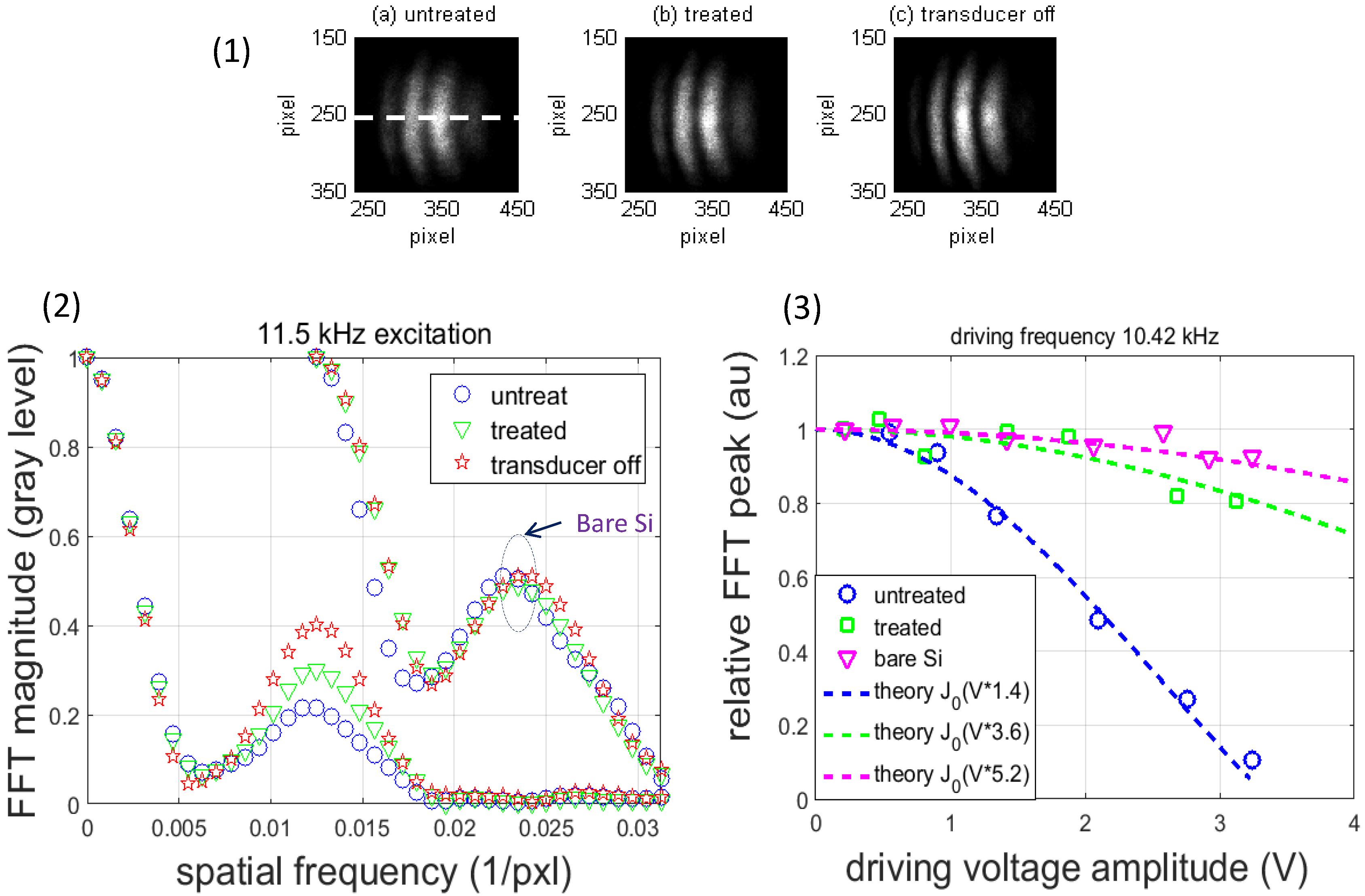
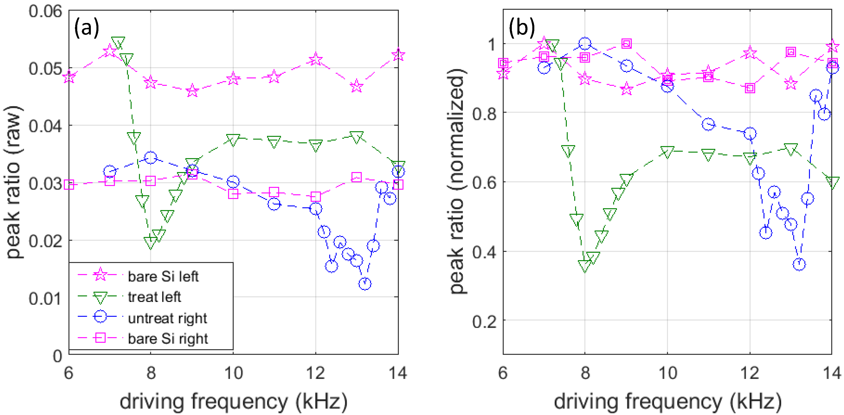
3.2.1. Treated and Untreated Specimens

Table 2. Specimens. T: film thickness; ρ: density of the film material; M: total film mass; mass ratio: the ratio of the square root of the mass of the Ti-Au and T-Pt films to that of the Ti film.

Film material	Ti	Ti-Au	Ti-Pt
T (nm)	75	$10/100$	$10/100$
ρ (kg/m${}^3$)	4510	4510/19,030	4510/21,450
M (kg)	$8.4\times {10}^{-9}$	$5.0\times {10}^{-8}$	$5.5\times {10}^{-8}$
mass ratio	1	$2.4$	$2.5$

summarizes the specimens used in this study. Each film material was coated on a silicon substrate ([1, 0, 0] plane) prepared with the pre-coating plasma treatment (the treated specimen) and on a silicon substrate of the same size without a pre-coating surface treatment (the untreated specimen). The films were initially coated on the silicon substrate as a disk of 75 mm in diameter and cut into an approximately 5 mm × 5 mm square specimen. The bottom row of this table shows the square root of the relative mass to the case of the Ti-only specimen. This quantity is called the mass ratio and will be used later in this section to estimate the resonant frequency of the interface. For dynamics associated with elastic force for a given elastic modulus in general, the resonant frequency is expected to vary inversely proportional to the square root of the mass.

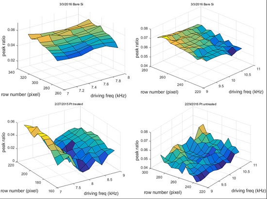
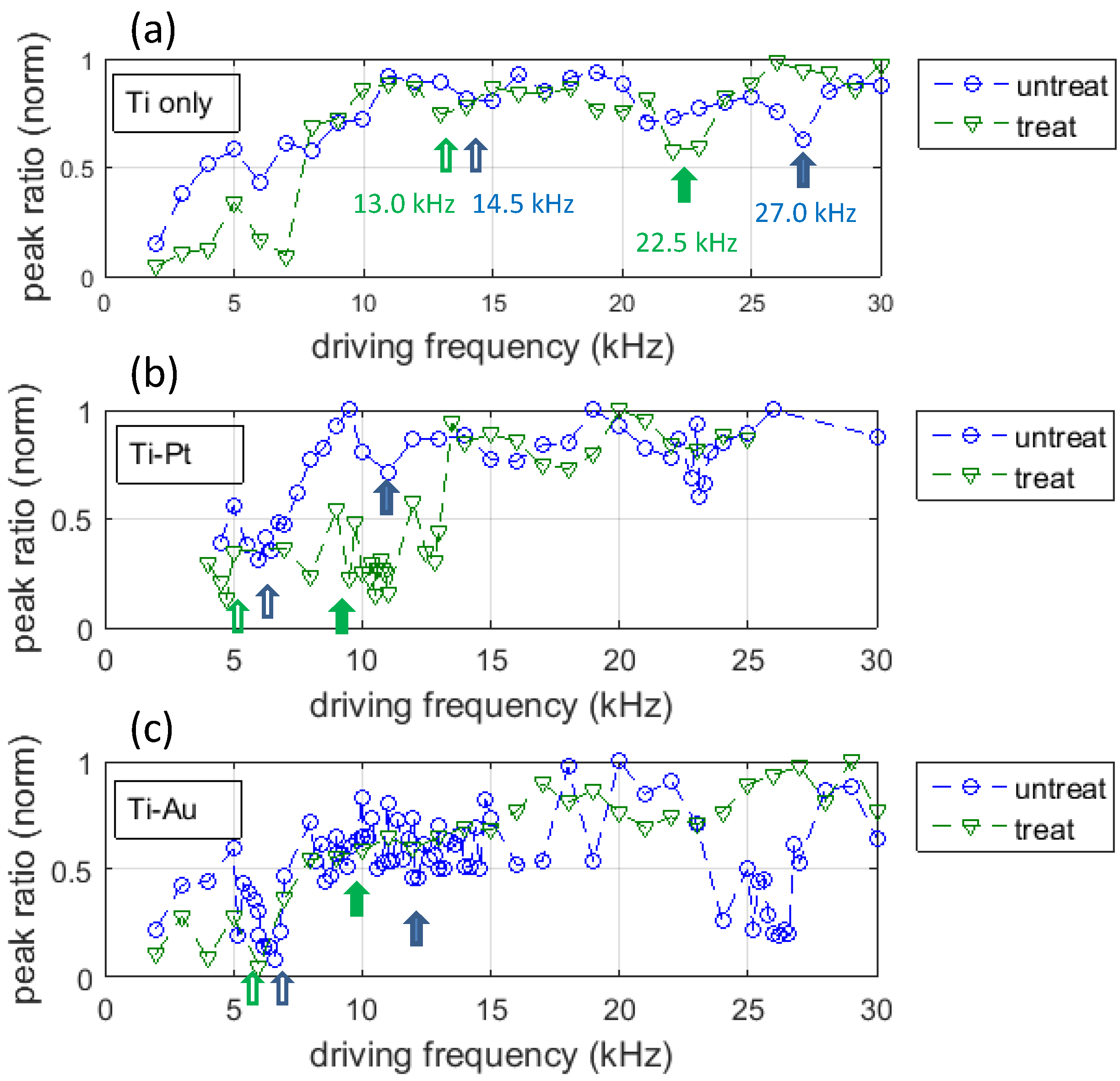
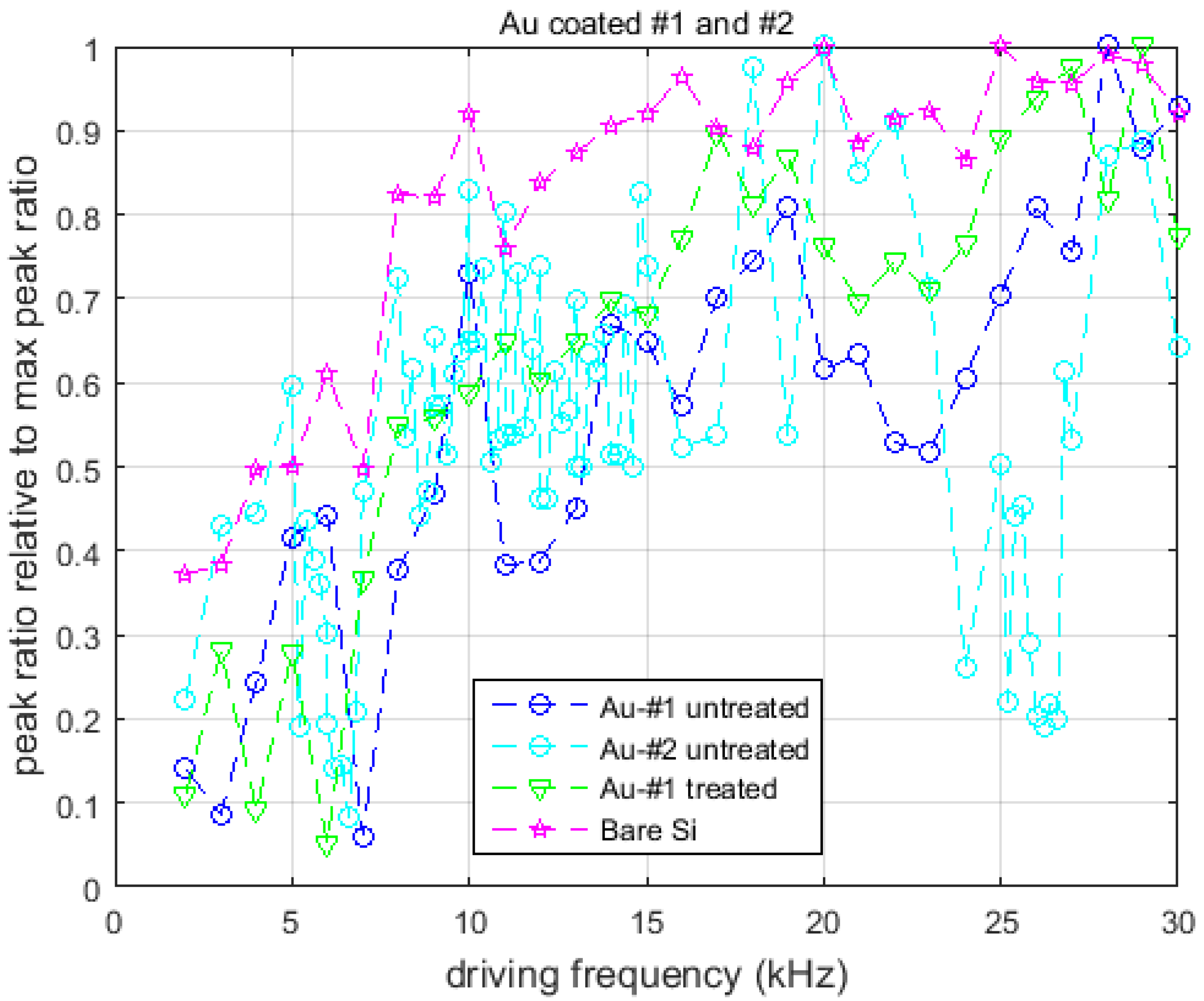
3.2.2. Observation of Resonance-Like Behavior

With the use of the interferometer setting shown in Figure 2, experiments were conducted numerous times with the treated and untreated thin-film specimens listed in Table 2. Figure 7 plots the peak value of the Fourier spectrum observed for each specimen as a function of the driving frequency (called the driving frequency sweep). For each specimen, the peak value is normalized to that of the bare silicon evaluated at the same driving frequency (called the peak ratio).

The driving frequency sweep of the peak ratio shows some features. In the Ti-only specimen case, the untreated specimen shows valleys around 14.5 kHz and 27 kHz (called the valley frequency). Similarly, the treated specimen shows valleys at 7 kHz, 13 kHz and 22.5 kHz. The higher valley frequencies observed in the respective specimens are approximately integer multiples of the lowest value. This indicates the possibility that the observed series of valley frequencies represents harmonics of the resonance for the respective specimen, being consistent with the above argument that the film-substrate interfaces have resonance in the swept frequency range. A previous study on Au-coated thin-film specimens clearly shows that the valley observed in the driving frequency sweep around the higher central frequency is the second harmonic of the valley observed around the lower central frequency [17].

Based on the assumption that the elastic property of the Ti-substrate interface is independent of the additional metal layers on top of the Ti layer and on the mass ratio shown in Table 2, the valley frequencies observed in the Ti-only case can be converted to the Ti-Pt and Ti-Au cases.

Table 3. Valley frequencies observed in Ti-only specimens and expected valley frequencies in Ti-Pt and Ti-Au specimens based on the mass ratio defined in Table 2 (unit: kHz).

Specimen	Valley 1		Valley 2
	Treated	Untreated	Treated	Untreated
Ti-only	13.0	14.5	22.5	27.0
Ti-Pt	5.2	5.8	9.0	10.8
Ti-Au	5.4	6.0	9.4	11.3

lists the valley frequencies estimated in this fashion for the Ti-Pt and Ti-Au specimens. In the driving frequency sweeps shown in Figure 7, the valley frequencies estimated for the Ti-Pt (b) and Ti-Au (c) specimens are indicated with arrows. Valleys are seen approximately at these estimated frequencies. In Table 3, the valley frequencies are grouped as Valley 1 and Valley 2. Valley 1 refers to the lower frequency pair of valley frequencies observed in the untreated and treated specimens of the same kind. Similarly, Valley 2 refers to the higher frequency pairs. Notice that in each pair, the valley frequency of the untreated specimen is 15% to 20% higher than the treated specimen. This is consistent with the results from the Doppler vibrometry shown in Table 1. These observations support the interpretation that the valleys in the driving frequency sweeps represent the resonance behaviors of the film-substrate interface.

The reduction in the fringe contrast, i.e., the peak ratio, is very sensitive to the optical alignment and other factors. The longer in the optical path that the interfering laser beams overlap each other, the greater the modulation depth ($J_0\left(\delta \right)$ in Equation (4)). The air flow near the interferometer and floor vibration also affect the fringe contrast. The driving frequency sweeps, the Ti-Pt case in particular, indicate that the data fluctuate vigorously near valleys. This is understandable if we consider the nature of the signal detected by the digital camera with the help of Equation (5). The Bessel function $J_0$ appearing in the second term of Equation (5) is steeper as the Fourier spectrum peak gets lower (Figure 3 (3)). This means that the greater the oscillation amplitude caused by the function generator, the more sensitive the spectrum peak becomes to the fluctuation of the voltage input to the transducer. The output voltage from the function generator used in the present study fluctuated approximately ±0.5% over the period of data taking for each driving frequency. To reduce those errors, we repeated the same measurement a number of times. The plots shown in Figure 7 are averages of over five measurements. The fluctuations in the peak ratio among these measurements were approximately ±5% near a valley frequency and ±2% in the frequency range away from valleys, respectively. From the slopes near valleys in Figure 7, the ±5% error in the peak ratio is translated into $<\pm$1% error in the valley frequency. Thus, the differences in the valley frequencies listed in Table 3 are significant.

In the case of the Ti-Au film, both the untreated and treated specimens show a significant reduction in the peak ratio. It is likely that this is because of poor adhesion between the Au and Ti films, rather than the poor adhesion between Ti and silicon substrate. Poor adhesion between Au and Ti layers was observed elsewhere in a film system similar to the present case [23].

3.2.3. Detailed Analysis on Ti-Pt Resonance

The observation of resonance-like behavior in the audible frequency range was somewhat surprising. In particular, the prominent valleys in the treated Ti-Pt specimen in the lower driving frequency range in Figure 7 was not expected. It was not observed in the previous study [17], where the lowest driving frequency was 10 kHz. We tested the Ti-Pt specimens a number of times using different interferometric setups with a similar interferometric setup in a different laboratory in a different country and still observed resonance-like behavior at the same frequency range. To confirm these observations more precisely, we made two modifications on the experimental arrangement. First, we added a second interferometric beam pair to the interferometer. This allowed us to take the measurement of two specimens simultaneously, thereby removing all temporal fluctuations common to the two interferometric pairs, such as intensity and polarization fluctuation of the laser beam and floor vibration noise, in comparing experimental data from the two specimens. Figure 8 illustrates the dual beam arrangement. The incident beam from the laser was split into two paths before the beam splitter of the interferometer. The two pairs of laser beams were delivered in parallel to each other to the end of the two interferometric arms. At the end of the X-arm (the horizontal arm in Figure 8), the first beam reflected off the first specimen, and the second beam reflected off the X-end mirror. At the end of the Y-arm (the vertical arm), the first beam reflected off the Y-end mirror and the second beam reflected off the second specimen.

Second, we calibrated the acoustic transducer by measuring the transducer’s oscillation amplitude as a function of the operating frequency and applied voltage. This ensured that the specimens were oscillated by the transducer with the same oscillation amplitude independent of the driving frequency. The constant transducer oscillation amplitude facilitated the measurement in the lower driving frequency end where the optical alignment was much more difficult than the higher frequency range because the oscillation amplitude was larger for the same applied voltage.

Figure 9a shows the raw data of the driving frequency sweep of the Fourier spectrum peak measured for the untreated and treated Ti-Pt specimens. Also shown in this figure are the Fourier spectrum peaks of a pair of bare Si specimens. One of the bare Si specimens was placed at the X-end of the interferometer, and the other was placed at the Y-end (Figure 8). The signal levels of the raw Fourier spectrum peak values for the two bare Si specimens are different because the first beam splitter did not split the laser beam exactly by 50%. Notice that the treated data converges to the bare Si data of the same arm at the low frequency end (7 kHz) and that the untreated data converges to the bare Si data of the same arm at the low and high frequency ends. This indicates that at these frequencies, the film surface oscillated for the same amount as the bare Si. In Figure 9b, the untreated and treated signals are normalized to the respective bare Si data. The valleys at 8 kHz in the treated specimen and those at 12.5 kHz and 13.5 kHz in the untreated specimen are more clearly seen than in Figure 9a.

3.2.4. Long-Term Temporal Change in the Valley Frequencies

In the course of the driving frequency sweep experiments, we noticed that the valley frequencies tended to shift after the specimen had been oscillated with the acoustic transducer for a certain amount of cumulative time. In some cases, the valley frequency increased and other times decreased. We have not understood this phenomenon on a solid physical basis yet, but it is worth presenting the findings at this time. Compare the lower valley observed in the Pt-Ti treated specimen observed in the driving frequency sweep in Figure 7 and the valley observed in the Pt-Ti treated specimen in Figure 9. This particular specimen was oscillated for approximately one year between the times that the two data were obtained. It is seen that the valley frequency had been shifted from approximately 11 kHz to 8 kHz. A similar phenomenon had been observed in the untreated Au-Ti specimen, as presented in Figure 10. In this figure, the data labeled #1 were taken after the specimen was oscillated for approximately one year, and the data labeled #2 were taken from a new specimen. The valley frequency of 22 kHz is seen to shift to 25 kHz. More investigation is currently being undertaken to explain this phenomenon.

3.2.5. Resonant Frequency

Based on the interpretation that the valley frequency represents the resonance of the elastic behavior of the interface and that the resonant frequency can be evaluated by taking the square root of the elastic constant of the film-substrate interface to the mass of the film, it is possible to compare the interfacial elasticity observed in this study with other studies.

Table 4. Valley frequencies and hypothetical resonant frequencies (unit: kHz). tr: treated specimen; untr: untreated specimen; pol. str: polystyrene specimen.

Ti-tr	Ti-untr	Ref. [2] Min	pol. str-tr	pol. str-untr	Ref. [2] Max	Ref. [24]
22.5	27.0	54.4	75.8	89.6	133.2	13,900

compares the valley frequency of the Ti specimen discussed above and the hypothetical resonant frequency calculated from the elastic constant found in the polystyrene specimen (Table 1) along with the interfacial elastic constant reported by Noijen et al. [2] and Ishiyama et al. [24]. Here, the hypothetical resonant frequency is calculated under the assumption that a 75 nm-thick, 5 mm × 5 mm Ti film is coated on the respective substrate. Noijen et al. [2] measured the interfacial elastic constant for a copper thin-film using the four-point bending test. Ishiyama et al. [24] measured the elastic constant of a columnar photoresist adhered to a silicon substrate.

Table 4 indicates that the resonant frequencies observed in this study are of the same order of magnitude as the Noijen’s four-point bending test. However, these are three orders of magnitude lower than the value estimated from Ishiyama’s measurement. These indicate the possibility that the above-observed resonance-like behaviors represent an elastic mechanism similar to the four-point test and fundamentally different from the column adhesion test. A possible mechanism to explain the elastic behavior observed in this study is discussed in the following section. It is interesting to note that Miyasaka [23] observed that the surface acoustic wave propagates at the interface of the Pt-Ti treated specimen (identical to this study) approximately 1.5% faster than the Pt-Ti untreated specimen (identical to this study) in his SAM experiment using a 400-MHz ultrasonic source. This indicates that the interfacial elastic constant of the treated specimen is higher than the untreated specimen, unlike our observation where the untreated specimen shows higher resonant frequency. It is possible that the 400-MHz acoustic wave probes the elastic mechanism represented by the elastic constant measured by the column test.

3.3. Possible Mechanism of the Observed Elastic Behavior

Although the mechanism behind the interfacial elastic dynamics responsible for the above-discussed resonance-like behaviors in the audible frequency range has not been understood, some arguments in association with the the phenomenon known as the interfacial blistering seem worth making. Thus, an attempt is made in this section to explain the experimental observation according to the following scenario. During the coating process, residual stresses are developed in the Ti layer. The residual stress either compresses or stretches the Ti layer parallel to the interface with the substrate and forms a pattern of compression and tension in the Ti layer. This pattern induces non-uniformity in the interfacial distance between the substrate and the Ti layer, generating a number of local, blister-like weak adhesions. The residual stress is not strong enough to cause delamination, but induces non-uniformity in the elastic strength. Volinsky et al. [25] discuss the effect of residual stress on thin aluminum films. Interfacial blistering is a major cause of delamination in the film-substrate interface and is usually discussed in the context of fracture mechanics. However, the dynamics of a blister in a thin-film’s interface seems to have resonance in the audible frequency range.

The details of interfacial blistering can be found elsewhere. In short, a blister can be formed in a film-substrate interfacial area where the adhesion is weaker than the surrounding area. Jensen [10] conducted a detailed study on the transition from the plate mode to the membrane mode dynamics in blister tests [12]. In blister tests, pressure is applied to the blistering area from the substrate side to inflate the film surface. When the height of the film-surface inflation reaches a critical value (relative to the film thickness), the elasticity of the film material takes over the longitudinal interfacial elasticity as the dominant restoring force mechanism of the blistering area; i.e., the elastic behavior of the area shifts from the plate mode to the membrane mode. In the present context, no pressure is applied to the film surface from the substrate side, and the structural condition of the interface is different from usual blister tests. However, if the applied dynamic load is at or close to the resonant frequency of the membrane-like elastic behavior, it is possible that the film surface bulges large enough to shift the elastic dynamics to membrane mode.

When a membrane is subject to a dynamic load, the membrane exhibits various oscillation modes, such as the drumhead mode. Each mode has its own resonant frequency that is related to the tension of the membrane, the density of the membrane material and the size of the membrane. In the case of the drumhead mode of a rectangular membrane, the resonant frequency is given by the following equation.

$$f_{mn}=\frac{1}{2}\sqrt{\frac{T}{\rho }[{\left(\frac{m}{a}\right)}^2+{\left(\frac{n}{b}\right)}^2]}$$

(12)

Here, $f_{mn}$ is the resonant frequency of the drumhead $mn$ mode; T is the membrane tension; ρ is the density of the membrane material; a and b are the sides of the membrane associated with modes m and n, respectively.

Apply the above idea to the Ti film of the present experiment. Since the tension of the film is unknown, Equation (12) cannot be used to estimate the resonant frequency. Therefore, here, we estimate the tension T from the observed valley frequency of 27 kHz (Table 3). The size of the laser beam forming a fringe pattern on the specimen is approximately 2 mm. Substitution of a = b = 2 mm, ρ = 4510 kg/m${}^3$ (Table 2) and m = n = 1 into Equation (12) leads to the tension corresponding to the lowest drumhead mode, 26 MPa. The tensile strength of Ti is approximately 1000 MPa, and the tension of 26 MPa corresponds to 2.6% of the tensile strength. Whether this value is reasonable or not for the tension of the present Ti film specimen cannot be argued from the information available in the present study. However, it is certainly not an impossible number. Residual stress can be tensile or compressive. The scenario of the membrane-mode dynamics in conjunction with residual stress on the Ti film and its relaxation to some extent explains the observation of the long-term effect that, in some cases, the valley frequency is increased and other times decreased after long runs.

To consider the possibility of the above mechanism in terms of the spatial profile of the adhesion weakness, we analyzed the peak ratio around the two valley frequencies observed in Figure 9 two-dimensionally. Figure 11 shows the peak-ratio valleys three-dimensionally for the treated and untreated specimens. Here, the horizontal axes are the driving frequency and the spatial coordinate axis perpendicular to the interferometric fringes. The valley in the untreated specimen appears circular as opposed to that in the treated specimen, which is more cylindrical. This indicates that in the direction parallel to the fringes, the treated specimen shows a wider area of weak adhesion than the untreated specimen. According to Equation (12), the resonant frequency is inversely proportional to the area. This difference in the size of the area possibly explains the fact that the treated valley frequency is lower than untreated. For analysis of the spatial profile of valleys in the orthogonal directions to Figure 11, the fringe systems must be rotated by 90${}^{\circ }$. This requires a major optical reconfiguration and is a subject of our future study.

4. Conclusions

Opto-acoustic methods to characterize the interface of thin-film systems were described. A thin-film system specimen was oscillated from the rear surface of the substrate in a range of audible frequencies, and the harmonic response of the film surface displacement was measured with a Doppler vibrometer and a Michelson interferometer. The choice of the acoustic frequency allowed us to oscillate the film and substrate as rigid bodies, so that the harmonic response represented the dynamics of the interface. The harmonic response was evaluated in the spatial frequency domain where the film surface oscillation was evaluated by the contrast of the interferometric fringes. Due to the fact that the frame rate of the digital camera that captured the interferometric images was much lower than the acoustic oscillation frequency, the oscillation amplitude decreased the fringe contrast. Theoretical consideration allowed us to relate the reduction in the fringe contrast to the oscillation amplitude using the zeroth order Bessel function of the first kind. Driving frequency sweeps of the fringe contrast measurement provided evidence that the interface had resonance in the tested audible frequency range.

Ti, Ti-Au and Ti-Pt thin-film coated on the same silicon substrate, along with the silicon substrate alone (the bare silicon) were tested with the Michelson interferometer. Each combination of film materials was coated on surface-treated and untreated silicon specimens separately. Comparison with the bare silicon specimen confirmed that the harmonic response of the film surface represented the dynamics of the interface. In each film material, both the untreated and treated specimens show resonance behavior where the resonant frequency of the untreated specimen was 15% to 20% higher than the treated specimen. Some of the observed resonant frequencies were found to shift over long-term use (oscillation) of the specimen.

The elastic constant associated with the observed resonant frequency was orders of magnitude lower than that of the film or substrate material. Neither a clear explanation for this finding nor the finding that the resonant frequency could shift after long-term use have been found. It is possible that the imperfection of chemical bonds in the interface drastically reduced the stiffness and/or that residual stresses induced during the coating process deformed the interface plastically, generating dislocations that reduced the elasticity. The resonant frequency shift seemed to be consistent with the explanation with residual stresses.

References

1. Turunen, M.P.K.; Marjamaki, P.; Paajanen, M.; Lahtinen, J.; Kivilahti, J.K. Pull-off test in the assessment of adhesion at printed wiring board metallization/epoxy interface. Microelectron. Reliab. 2004, 44, 993–1007. [Google Scholar] [CrossRef]
2. Noijenh, S.P.M.; van der Sluis, O.; Timmermans, P.H.M. An Extensive Investigation of the Four Point Bending Test for Interface Characterization. In Proceedings of the 13th International Conference on Thermal, Mechanical and Multi-Physics Simulation and Experiments in Microelectronics and Microsystems, EuroSimE, Cascais, Portugal, 16–18 April 2012.
3. Laugier, M.T. An energy approach to the adhesion of coatings using the scratch test. Thin Solid Films 1984, 117, 243–249. [Google Scholar] [CrossRef]
4. Bunett, P.J.; Rickerby, D.S. The scratch adhesion test: An elastic-plastic indentation analysis. Thin Solid Films 1988, 157, 233–244. [Google Scholar] [CrossRef]
5. Lemons, R.A.; Quate, C.F. Acoustic microscopy. In Physical Acoustics; Mason, W.P., Thurston, R.N., Eds.; Academic Press: London, UK, 1979; Volume XIV, pp. 1–92. [Google Scholar]
6. Weglein, R.D. Acoustic microscopy applied to SAW dispersion and film thickness measurement. IEEE Trans. Sonics 1980, 27, 82–86. [Google Scholar] [CrossRef]
7. Atalar, A. An angular-spectrum approach to contrast in reflection acoustic microscopy. J. Appl. Phys. 1978, 49, 1530–1539. [Google Scholar] [CrossRef]
8. Atalar, A. A physical model for acoustic signatures. J. Appl. Phys. 1979, 50, 8237–8239. [Google Scholar] [CrossRef]
9. Telschow, K.L.; Deason, V.A.; Cottle, D.L.; Larson, J.D., III. Full-field imaging of gigahertz film bulk acoustic resonator motion. IEEE Trans. Ultrason. 2003, 50, 1279–1285. [Google Scholar] [CrossRef]
10. Jensen, H.M. Analysis of mode mixity in blister test. Int. J. Fract. 1988, 94, 79–88. [Google Scholar] [CrossRef]
11. Bedrossian, J.; Kohn, R.V. Blister patterns and energy minimization in compressed thin films on compliant substrates. Commun. Pure Appl. Math. 2015, 68, 472–510. [Google Scholar] [CrossRef]
12. Dennenberg, H. Measurement of adhesion by a blister method. J. Appl. Ploym. Sci. 1961, 5, 125–134. [Google Scholar] [CrossRef]
13. Volinsky, A.A.; Moody, N.R.; Gerberich, W.W. Interfacial toughness measurements for thin films on substrates. Acta Mater. 2002, 50, 441–466. [Google Scholar] [CrossRef]
14. Liao, Q.; Fu, J.; Jin, X. Single-chain polystyrene particles adsorbed on the silicon surface: A molecular dynamics simulation. Langmuir 1999, 15, 7795–7801. [Google Scholar] [CrossRef]
15. Huang, C.; Ma, C. Vibration characteristics for piezoelectric cylinders using amplitude- fluctuation electronic speckle pattern Interferometry. AIAA J. 1988, 36, 2262–2268. [Google Scholar] [CrossRef]
16. Wang, W.C.; Hwang, C.H. The Development and Applications of Amplitude Fluctuation Electronic Speckle Pattern Interferometry Method. In Recent Advances in Mechanics; Kounadis, A.N., Gdoutos, E.E., Eds.; Springer: New York, NY, USA, 2011; pp. 343–358. [Google Scholar]
17. Yoshida, S.; Adhikari, S.; Gomi, K.; Shrestha, R.; Huggett, D.; Miyasaka, C.; Park, I.K. Opto-acoustic technique to evaluate adhesion strength of thin-film systems. AIP Adv. 2012, 2, 022126:1–022126:7. [Google Scholar] [CrossRef]
18. Yoshida, S.; Didie, D.R.; Didie, D.; Adhikari, S.; Park, I.K. Opto-Acoustic Technique to Investigate Interface of Thin-Film Systems. In Advancement of Optical Methods in Experimental Mechanics; Jin, H., Sciammarella, C., Yoshida, S., Laberti, L., Eds.; Springer: New York, NY, USA, 2014; Volume 3, pp. 117–125. [Google Scholar]
19. OFV-5000 Vibrometer Controller. Available online: http://www.polytec.com/us/products/vibration-sensors/single-point-vibrometers/ modular-systems/ofv-5000-vibrometer-controller/ (accessed on 11 May 2016).
20. DD-300 24 MHz Dispolacement Decoder. Available online: http://www.polytec.com/fileadmin/user_uploads/Products/Vibrometers/OFV-Decoder/Displacement_Decoder/Documents/OM_DS_DD-300_2010_07_PDF_E.pdf (accessed on 11 May 2016).
21. Basnet, M.; Yoshida, S.; Tittmann, B.R.; Kalkan, A.K.; Miyasaka, C. Quantitative Nondestructive Evaluation for Adhesive Strength at an Interface of a Thin Film System with Opto-Acoustic Techniques. In Proceedings of the 47th Annual Technical Meeting of Society of Engineering Science, Ames, IA, USA, 4–6 October 2010.
22. Scalise, L.; Paone, N. Laser Doppler vibrometry based on self-mixing effect. Opt. Lasers Eng. 2002, 38, 173–184. [Google Scholar] [CrossRef]
23. Miyasaka, C.; Pennsylvania State University, University Park, PA, USA. Personal communication, 2012.
24. Ishiyama, C.; Tasaki, T.; Tso-Fu Mark Chan, T.M.; Sone, M. Effects of specimen dimensions on adhesive shear strength between a microsized SU-8 column and a silicon substrate. Jpn. J. Appl. Phys. 2012, 51. [Google Scholar] [CrossRef]
25. Volinsky, A.A.; Moody, N.R.; Gerberich, W.W. Superlayer residual stress effect on the indentation adhesion measurement. Mater. Res. Soc. Proc. 2000, 594, 383–388. [Google Scholar] [CrossRef]
Figure 1. Physical model of thin-film systems. The figures at the bottom show the membrane-like vibration of the film surface due to the weaker elastic constant of the middle part.
Applsci 06 00163 g001
Figure 2. Experimental arrangement with a Michelson-type interferometer. The function generator (Gold Star Model FG 8002) sends sinusoidal input voltage to the acoustic transducer (magnetic type, Design Factory Dokodemo-Speaker 8297).
Applsci 06 00163 g002
Figure 3. (1) Examples of fringe patterns; (2) Fourier spectra of intensity along the horizontal line indicated in Fringe Pattern (a); and (3) driving-voltage dependence of spectral peak value relative to the transducer-off (null driving voltage) case.
Applsci 06 00163 g003
Figure 4. Doppler vibrometry setup.
Applsci 06 00163 g004
Figure 5. Signal from Doppler vibrometry.
Applsci 06 00163 g005
Figure 6. Assimilation of observed relative amplitude and phase with harmonic response function Equations (10) and (11).
Applsci 06 00163 g006
Figure 7. Peak ratio as a function of driving frequency. The valley frequencies indicated in (a) the Ti-only specimen are measured values. The valley frequencies pointed to by arrows in (b) Ti-Pt and (c) Ti-Au indicate valley frequencies estimated from those in (a) and the mass ratio defined in Table 2.
Applsci 06 00163 g007
Figure 8. Dual beam Michelson interferometer. Beam Splitter 1 (BS1) splits the incoming laser beam into two passes for two pairs of interferences. Beam 2 is reflected on the rear surface of BS1. Light reflected on the Si/Pt specimen surface interferes with light reflected on M2/M1. Two interferometric fringe patterns are formed on the screen simultaneously. Respective specimens and corresponding mirrors are aligned for fringe formation, as explained in Figure 2. The screen is placed at a distance for better alignment of interfering light beams.
Applsci 06 00163 g008
Figure 9. Valley frequencies of untreated, treated Pt-Ti specimens and bare Si specimens. (a) Raw data of peak ratio; (b) normalized to the bare Si data for the respective mirrors, i.e., the Pt-Ti specimen data obtained with the right/left mirror to bare Si data with the right/left mirror.
Applsci 06 00163 g009
Figure 10. Valley frequency shift observed in the Ti-Au untreated specimen.
Applsci 06 00163 g010
Figure 11. Three-dimensional plots of resonance-like peaks.
Applsci 06 00163 g011