A Novel Health Factor to Predict the Battery’s State-of-Health Using a Support Vector Machine Approach

Abstract

The maximum available capacity is an important indicator for determining the State-of-Health (SOH) of a lithium-ion battery. Upon analyzing the experimental results of the cycle life and open circuit voltage tests, a novel health factor which can be used to characterize the maximum available capacity was proposed to predict the battery’s SOH. The health factor proposed contains the features extracted from the terminal voltage drop during the battery rest. In real applications, obtaining such health factor has the following advantages. The battery only needs to have a rest after it is charged or discharged, it is easy to implement. Charging or discharging a battery to a specific voltage rather than a specific state of charge which is difficult to obtain the accurate value, so the health factor has high accuracy. The health factor is not dependent on the cycle number of the cycle life test of the battery and it is less dependent on charging or discharging current rate, as a result, the working conditions have less effect on the health factor. Further, the paper adopted a support vector machine approach to connect the healthy factor to the maximum available battery capacity of the battery. The experimental results show that the proposed method can predict the SOH of the battery well.

1. Introduction

Energy is the basis of the human survival and development. The growing concern over oil shortage and environmental issues has greatly accelerated the development of green energy to replace fossil fuel in recent years [1]. Since transportation consumes a large part of energy, to develop and apply electric vehicles (EV) is necessary in the way of green mobility [2]. It is well known that the battery pack is the key component of EV, hybrid electric vehicles (HEV) and plug-in hybrid electric vehicles (PHEV). Lithium-ion battery (LIB) is for the high specific or volumetric power and energy density, high cycle lifetime and decreasing cost have made them more attractive for the vehicles [3]. The reliable and efficient battery management systems need to be developed to ensure the power battery work well [4,5], estimating the state-of-health (SOH) of the battery is the most crucial function among the various functions of a battery management system [6].

The SOH is a metric of the battery’s age that reflects the ability of a battery to store and deliver energy relative to initial condition. However, the degradation of a LIB is a very complex process that is affected by many factors, such as charge/discharge rate, storage temperature and operating process. Compared with the state of charge (SOC) estimation, the SOH estimation is more challenging [7]. In practical applications, the degradation of the battery causes many parameters such as battery capacity and battery impedance to change. The quantitative definition of the SOH is mainly based on the internal resistance increase or the capacity degradation.

The SOH estimating methods based on internal resistance increase needs to get the initial resistance when the battery is fresh and the resistance at the end-of-life (EOL). When the resistance changed with aging of the battery is achieved, it could estimate the SOH of the battery. The traditional method to get the parameters of the battery is electrochemical impedance spectrum (EIS), which is a powerful lab-based diagnostic technique. However, the principle of the EIS method is to apply to a cell a sinusoidal signal and measure the characteristic response from the cell, it is not suitable for the real application. The aim of the EIS is to improve the speed of the calculation [8] and make use of the free signals of current and voltage during the operation of the battery instead of the additional burden of the input signal, so as to carry out SOH estimation in real time [9,10]. Moreover, Equivalent Circuit Models (ECMs) can simulate the static and dynamic behavior of a battery. It is commonly used to predict the SOH by identifying the resistance of the equivalent circuit models (ECMs). However, different ECMs, different parameter identification methods and different battery operating conditions will affect the precision of the parameter identification. Improving the precision of the parameter identification is the key problem to be addressed.

The SOH estimating methods based on capacity degradation needs to get the maximum available capacity which changes with aging of the battery. The ratio of the maximum available capacity and the nominal capacity is the SOH of the battery. When the current maximum available capacity is reduced to 80% of the nominal capacity of the battery, it is considered to have reached the EOL of the battery [11]. Among all the methods based on capacity degradation, the most direct way is to discharge the battery from the fully charged state to the discharge cutoff voltage at a specified current rate and ambient temperature. The number of ampere-hours drawn from the battery under such working condition is the maximum available capacity of the battery [12,13]. This method is simple and direct but it is not suitable for practical applications. Thus, the aim of the improvement is to estimate the SOH in real time for a part cycle and dynamic condition instead of for the whole cycle and a constant condition. This study uses the capacity degradation method to estimate SOH and the contributions are as follows:

• The experimental data of the battery cycle life and open circuit voltage (OCV) are studied. Upon analyzing the data, it is concluded that the degradation of the battery causes OCV variation and the instantaneous voltage drop of the terminal voltage rises along with the increasing cycle numbers.
• A novel health factor extracted from the terminal voltage drop is proposed to estimate the available capacity of the battery that can indicate the SOH of the battery. Furthermore, a support vector machine (SVM) approach is used to build the relationship between the health factor and available capacity of the battery. The experimental result showed that the method has high precision.
• The reason for selecting the terminal voltage drop information as the health factor is analyzed and its performance is verified. The study explained why charging or discharging a battery to a certain voltage is superior to charging or discharging the battery to a certain SOC. Moreover, the SOH estimating results showed that the method is not limited to the working conditions of the battery.
• The modeling precision using different features of the terminal voltage drop as the health factor is compared. Furthermore, the effectiveness of the model is verified and analyzed.

The remainder of the study is organized as follows: an overview of the capacity estimation methods is shown in Section 2. In Section 3, the design of the experiments for the cycling test of the battery is introduced and the results are analyzed. In Section 4, a SVM is used to establish the relationship between the available capacity of the battery and its terminal voltage drop. Thereafter, in Section 5, the results of the prediction method based on the SVM are showed and analyzed. Finally, this work is summarized.

2. SOH Definition and Computation

The SOH based on capacity degradation is usually defined as [14,15]:

$$SOH=\frac{Q_i}{Q_C}\times 100\%$$

(1)

where, Q_i is the maximum available capacity at a certain time i. It is defined in Equation (2). Q_i represents the total number of ampere-hours can be drawn from the fully charged battery at a specified current rate and ambient temperature. Q_c is the nominal capacity of the battery.

$$Q_i=\frac{1}{3600}{\displaystyle {\int }_0^{T_i}\eta \cdot i(t)dt}$$

(2)

where, time 0 means the initial discharge time and T_i means the end of the discharge time. $\eta$ represents the coulombic efficiency and t is in seconds. At present, the mainstream methods of available capacity are as following [16]:

(1) The methods based on OCV and more strictly based on the electro motive force (EMF) [17], that is, using the relationship between the EMF and the SOC to estimate the SOH of the battery while in idle or in operation.

These methods are based on the following Equation:

$$\frac{1}{3600}{\displaystyle {\int }_{t_1}^{t_2}\eta \cdot i(t)dt=C\cdot (SOC(t_2)-SOC(t_1))}$$

(3)

An equivalent Equation to (3) is shown in (4):

$$C=\frac{1}{3600}{\displaystyle {\int }_{t_1}^{t_2}\eta \cdot i(t)dt/(SOC(t_2)-SOC(t_1))}$$

(4)

where, SOC (t) means the SOC value at time t.

Upon measuring the OCV value of the certain time t₁ and t₂, the SOC value of certain times t₁ and t₂ can be calculated based on the OCV-SOC curve. Thus, the available capacity of the battery can be predicted according to the abovementioned Equation (4). After charging or discharging the battery, it needs to rest for a relatively long time. That is, to measure OCV precisely, the battery should be in a completely steady state [18]. Therefore, improvements to this type of methods are focused on how to calculate the OCV (or EMF) in a short relaxation time or without a relaxation time and how to improve the accuracy of the OCV-SOC curve [19,20].

Pei et al. [21] put forward a rapid OCV prediction method to predict the final static OCV using linear regression techniques, based on a novel mathematical model developed from an improvement on a second-order resistance-capacitance (RC) model [1]. Weng et al. [22] proposed a novel OCV model which has a much better fitting accuracy for considering the staging phenomenon during the lithium intercalation/deintercalation process for LIB. Tong et al. [23] proposed a SOH (SOC) correction as part of the battery equivalent circuit model (ECM) and on-line optimization of SOH (SOC) correlation impelled to optimize the OCV- SOC correlation and the capacity of a LIB. Farmann et al. [24] shows that the main factors influencing the OCV behavior of LIB are aging, temperature and working history of the battery. Furthermore, the paper investigated the impact of the abovementioned factors on OCV at different aging states using various active materials (C/NMC, C.LEP, LTO/NMC) over a wide temperature range (−20 °C–45 °C).

(2) The methods based on incremental capacity analysis (ICA) and differential voltage analysis (DVA).

These methods use the electrochemical characteristics of the battery. For ICA, the obtained curves V-dQ/dV transform the plateau present in the cell voltage trend (representative of electrochemical equilibrium phases during the cell operation) into peaks [25,26]. For DVA, the obtained trend Q-dV/dQ presents, for each peak, the transition between two electrochemical equilibrium conditions during the battery operation conditions [27]. The locations and amplitudes of such peaks can reflect the deterioration of the battery. For the measured voltage contains trembling and noise, as a result, the perturbation is introduced into the IC or DV curves which make it difficult to identify the peaks. This kind of method makes full use of the electrochemical characteristics of the battery. However, it has strict requirements regarding the operating conditions. For example, charging or discharging with a Constant Current (CC) in a large voltage range (contained at least the peak voltage) and the CC should be small enough to sufficiently show the voltage plateau [28]. Furthermore, all the peaks on the IC curve lie within the voltage plateau region of the V-Q (Voltage-Capacity) curve [29], which is relatively flat and more sensitive to measurement noise. Hence, effective and robust algorithms of obtaining the IC and DV curve need to be developed.

Feng et al. [30] proposed a probability density function (PDF), which has an equivalence performance with ICA/DVA for predicting the SOH. Wang et al. [31] presented an algorithm to obtain the DV curve according to the center least squares used the location interval between two influence points or the transformation parameter of the DV curve, as a result, the error was within 2.5%. Li et al. [32] proposed a simple and robust smoothing method based on Gaussian filter to reduce the noise on IC curves. Zheng et al. [33] presented a SOC based ICA/DVA method to address the question, that is, the conventional cell terminal voltage based ICA/DVA methods are sensitive to the changed resistance and polarization during battery aging processes.

(3) Methods based on data-driving

This type of methods is aimed to find degradation mechanism of a battery by analyzing the characteristic data without considering its electrochemical reaction and failure mechanism [34]. The data that can reflect the characteristics of the battery SOH and its evolution is called health factor [35]. This method will establish the relationship between the experiment data and battery degradation to diagnose and estimate the SOH of the battery [36]. Since the SOH of the battery is bound to be reflected by its external charge and discharge characteristics, thus this type of method does not consider the internal characteristics of the battery [37].

You et al. [38] proposed a data-driven approach to trace SOH on the fly by using current, voltage and temperature while leveraging their historical distributions. When it is used under actual EV driving conditions, the average error is less than 2.18%. Tong et al. [23] put forward a SOH prediction method based on the health factor constructed through OCV of the battery. It can effectively track the SOH. However, it takes a long time to get the OCV value and is hard to implement online. Liu et al. [39] and Widodo et al. [40] used voltage drop of same time and the same voltage drop in each cycle life test as health factors respectively. This method needs to work under constant current discharge conditions to achieve the health factor. Wei et al. [41] proposed a health factor characterized by increment of Ohmic internal resistance, increment of polarization internal resistance and the reduction of polarization capacitance to realize online SOH prediction. The main problem of this type of methods is that the battery has to be discharged or has to work under specific operating conditions, such as under cycle life test conditions, to obtain the health factor. It is known that additional discharging is detrimental to the battery and that, when the battery is actually used, the operating conditions are dynamic.

Aforementioned, a novel SOH estimation method adopting the relative features of the terminal voltage drop as the health factor is proposed. The battery only needs to be charged to get the health factor and the operating conditions are not restricted.

3. Design and Result Analysis of the Battery Cycle Life Test

This section includes three parts: first, the experiment platform is introduced. The life cycle experiment and the OCV-SOC experiment are introduced in second part. The third part analyzes the experimental data and draws a conclusion that the available capacity of the LIB under test decreases with the life and the voltage drop of terminal voltage increases with life. It further analyzes the advantage of charging or discharging the battery to a certain voltage instead of charging or discharging it to a certain SOC.

3.1. Experimental Platform

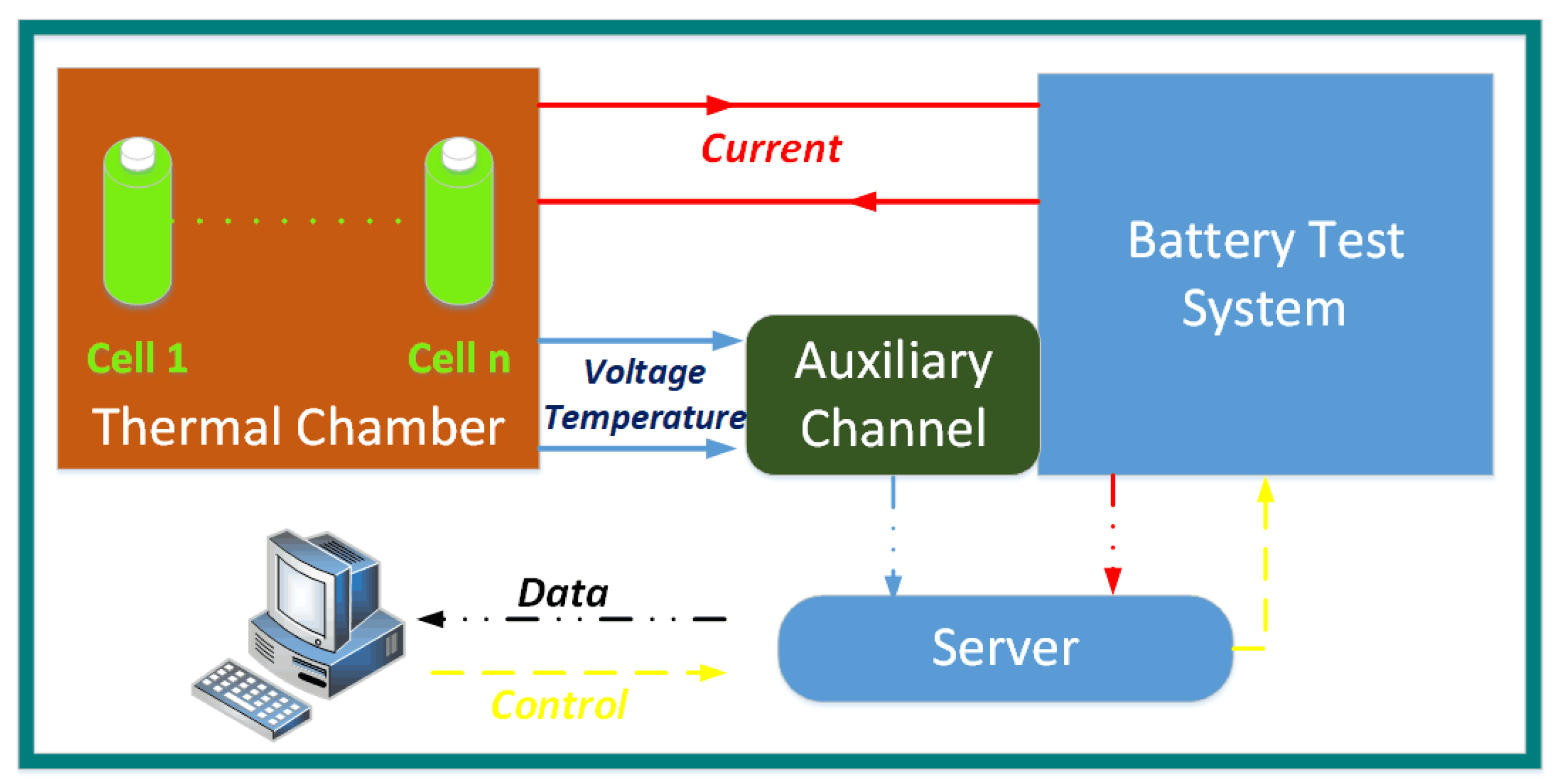
The experimental platform is shown in Figure 1 and it mainly contains a NEWARE BTS-4008 power battery test system, a controlled thermal chamber and a computer. During the experiment, the batteries are put in the controlled thermal chamber and the computer is used to control the experimental platform by server, to set the operating condition and save the experiment data. In this study, commercially available cylindrical 18650-type lithium-ion cells (Lithium nickel–manganese–cobalt oxide/ Graphite) were investigated. The performance of the battery is showed in

Table 1. Main specifications of the tested battery.

Nominal Capacity	Nominal Voltage	Charging Cutoff Voltage	Discharging Cutoff Voltage
1500 mAh	3.7 V	4.2 V	2.5 V

. In experiments, the cells are numbered. In this paper, the No. 1 battery is used for analysis and modeling and the No. 2 battery with the same type is used to verify the efficiency of the method.

3.2. Experimental Procedure

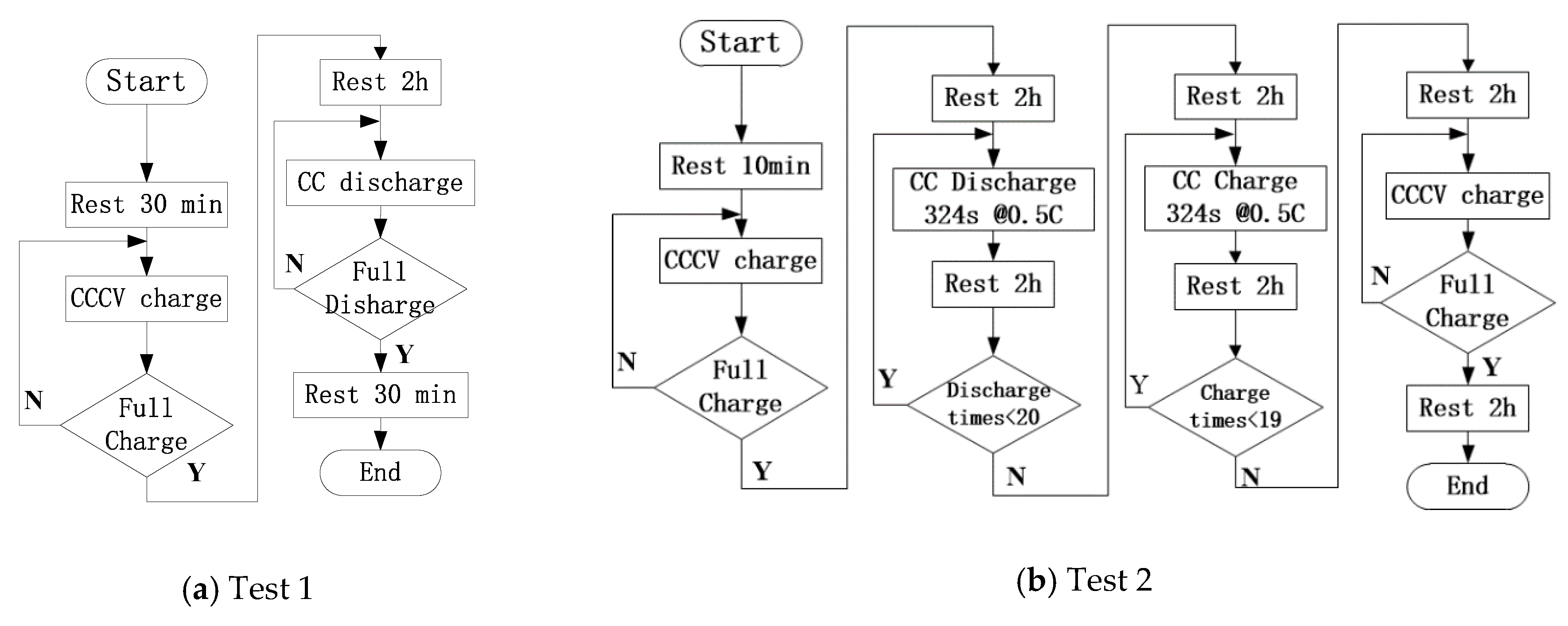
Cycle life and OCV tests [42] of the batteries were carried out at room temperature, in which the cycle life test, also called Test 1, is the main experiment and after 80-100 cycle tests, an OCV test, also called Test 2, was performed to obtain the OCV-SOC curves for different degrees of aging of the batteries.

Test 1: Cycle life test, the steps of one cycle life test are as follows:

(1) The battery rests for 30 min before the cycle life test.

(2) The battery is charged in the standard constant current constant voltage (CCCV) mode. CCCV means that the battery is charged with a CC until the charging cutoff voltage and a constant voltage (CV) is used to charge until the current is reduced to a predefined current. The CC is 750 mA, the charging cutoff voltage is 4.2 V and the charging is ended when the current is reduced to 20 mA under the cutoff voltage.

(3) The battery has rests for 30 min.

(4) The battery is discharged in the CC mode until the discharging cutoff voltage, at which the CC is 750 mA and the discharging cutoff voltage is 2.5 V.

(5) The battery rests for 30 min.

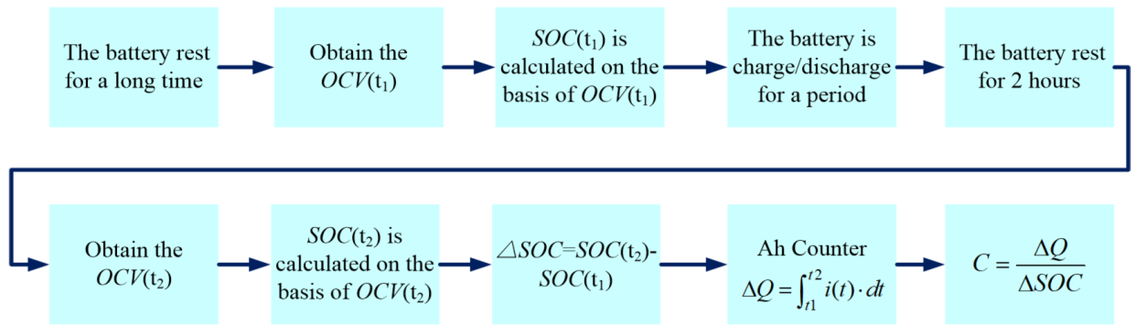
Test 2: OCV test to obtain the OCV-SOC curve. A flowchart of the experiment is showed in Figure 2 and the steps of one cycle life test are as follows:

(1) The battery is charged to fully state in the standard constant current constant voltage (CCCV) mode just like test 1 and then it will rest for 2 h.

(2) The battery continues 20 cycles, that is, the battery is discharged in CC mode for 324 s and then rests for 2 h.

(3) The battery continues 19 cycles, that is, the battery is charged in CC mode for 324s and then rests for 2 h.

(4) The battery is charged to fully state in the standard constant current constant voltage (CCCV) mode just like test 1 and then it will rest for 2 h.

In test 2, CC and CCCV have the same meaning with the test 1.

3.3. Experimental Results and Analysis

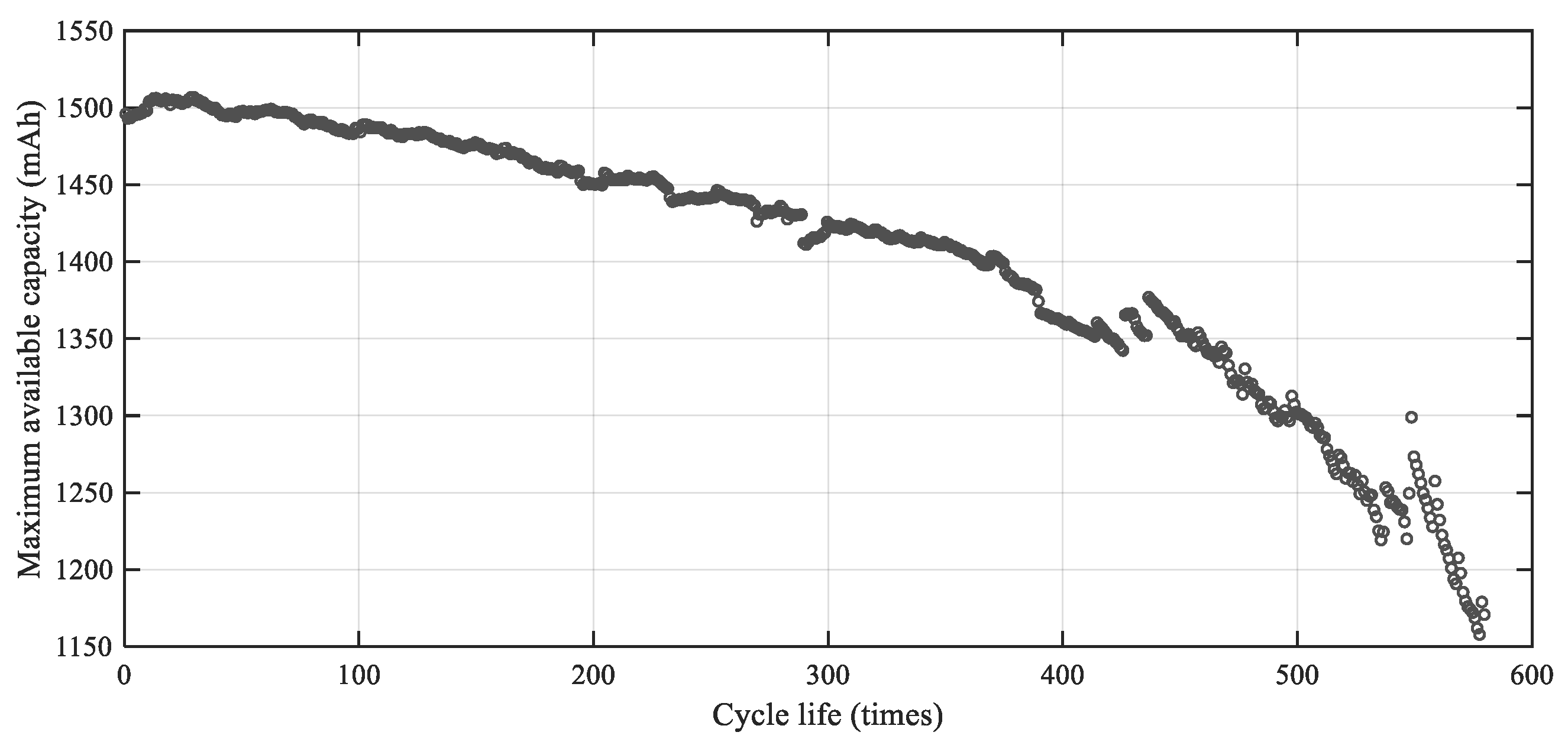
The cycle life test and the OCV test continued until the available capacity of the aging battery is less than 80% of the nominal capacity. The experimental results of the No. 1 battery are shown in Figure 3, Figure 4, Figure 5 and Figure 6. The relationship between the available capacity and the cycle number of the cycle life test is shown in Figure 3. It should be noted that the amount discharged under such a cycle life test is considered to be the available capacity of the battery.

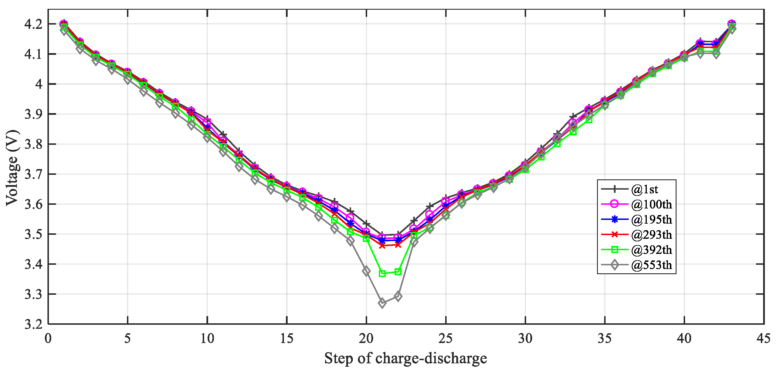
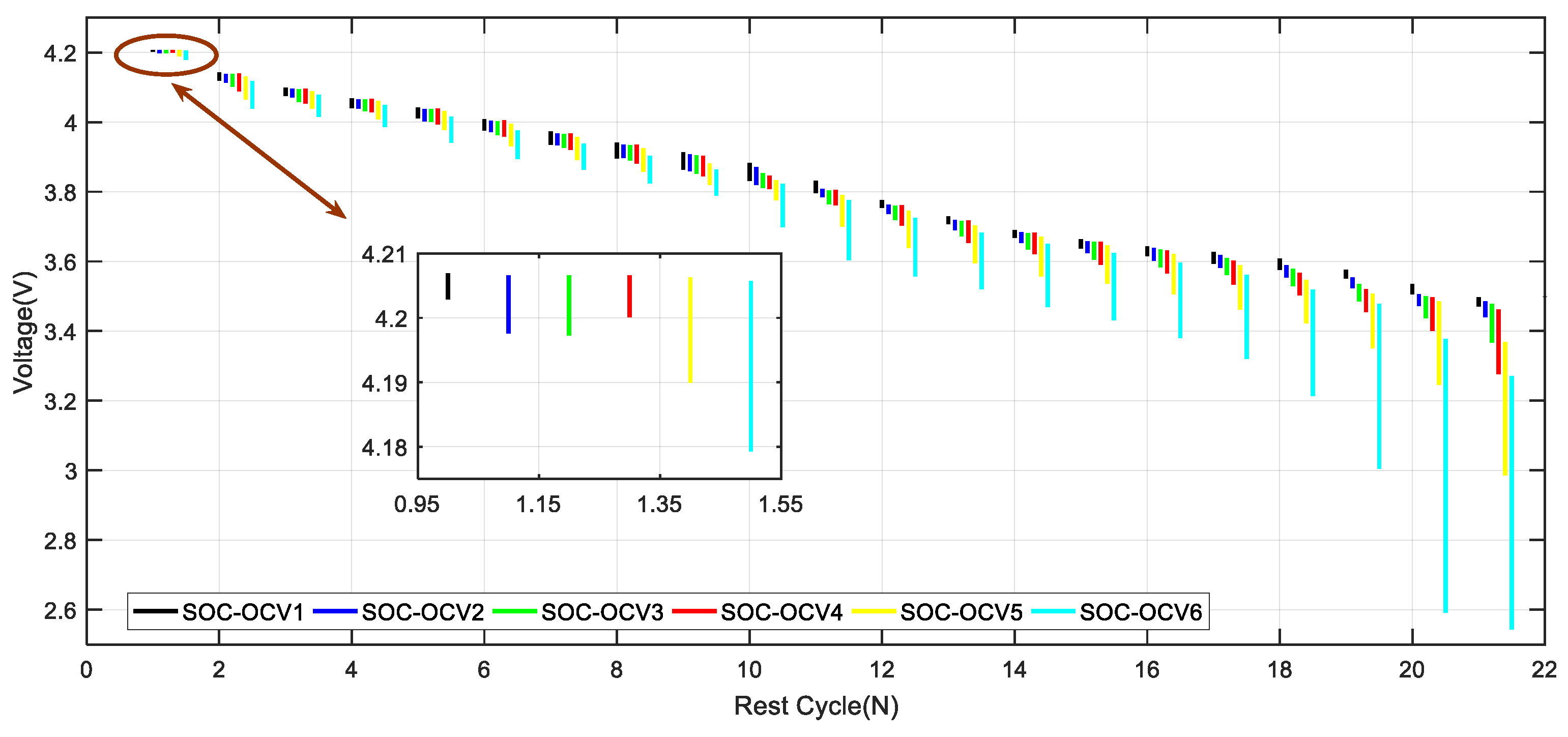
Six OCV test for different cycle numbers are shown in Figure 4. The ith time indicates that the corresponding OCV data is obtained after the ith time of the cycle life test.

Figure 5 showed the terminal voltage drop when the fully charged battery has a rest for 2 h and the terminal voltage drops when the discharged battery has a rest for 2 h for the six OCV test.

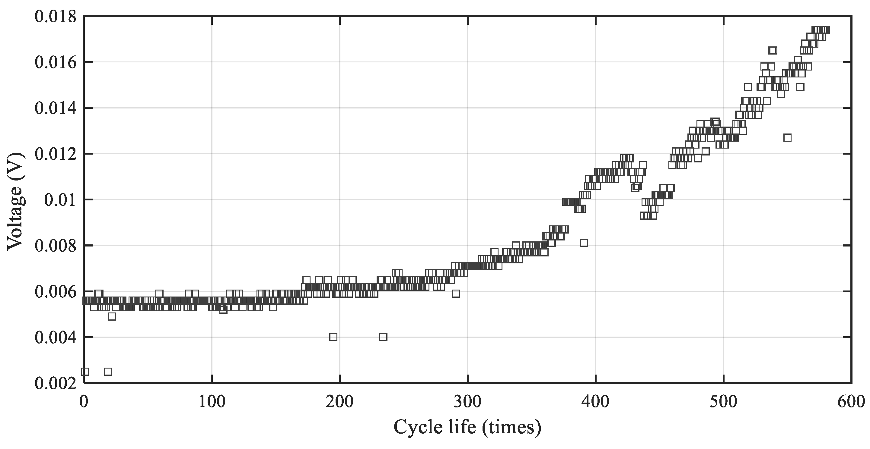
Figure 6 showed the terminal voltage drop after the fully charged battery rested for 30 min; here, a fully charged battery means that the battery is charged with the CC until the charging cutoff voltage and goes on to be charged in the CV mode until the current is reduced to 20 mA, just like in the illustration in Section 3.2.

The following can be inferred by analyzed the experiment results.

(1) Figure 3 presented that with the increasing number of cycles, although the amount discharged (i.e., the available capacity of the battery) is not monotonically attenuated, the overall trend is decreasing. On the other hand, compared with the early life stage (for example, the 1–200 cycle), the capacity decreases rapidly at the later stage of life (for example, cycle > 400).

(2) Figure 4 showed that the six OCV test is operated under the same working condition, the results are different. The battery has a rest for two hours after it reaches fully charged state in CV mode. The terminal voltage of the battery is gradually decreasing as the number of cycles increases. The charging process also has a similar regular pattern.

(3) Figure 5 presented that during the discharging, even with the same discharging current, the same discharging time, when the battery is stopped charging and rests for the same time (i.e., two hours in this study), the terminal voltage drop of the battery is gradually increasing with the degradation of the battery. The value of the terminal voltage drop is relative to SOC value and the lower the SOC value, the greater the terminal voltage drop. Terminal voltage is no longer changing, it can be regarded as the OCV of the battery. Conversely, the decreasing battery capacity leads to the changes in the thermodynamic and kinetic characteristics of battery and the corresponding relationship between the available capacity and OCV is the direct external embodiment of thermodynamic characteristics of battery [43]. Thus, the capacity degradation causes a change in the OCV, that is, the value of the terminal voltage drop with the same rest time can reflect the degradation of the available capacity.

(4) Figure 6 showed that with the increasing number of cycles, after the fully charged battery has rested for 30 min and compared with the initial terminal voltage at the moment when the battery is just fully charged, the terminal voltage drop does not increase monotonously but the overall trend is increasing. The terminal voltage drop is trending in the opposite direction to the change in the available capacity of the battery combined with Figure 3.

In addition, the following must be taken into account:

(1) It is difficult to get precise SOC values.

Equation (5) is generally used to calculate the SOC of the battery:

$$SOC=1-\frac{Q_t}{Q_{all}}=1-\frac{{\displaystyle {\int }_0^{t}i(\tau )}d\tau }{{\displaystyle {\int }_0^{T}i(\tau )d\tau }}$$

(5)

The Q_t represents the amount discharged from the beginning of the discharging (the fully charged battery) to the moment t, Q_all represents the amount discharged from the fully charged battery to the cut-off voltage. T represents the whole discharging duration. In real application, we can get Q_t easily but the Q_all cannot be measured at the moment t if the battery is not out of power. Hence, the nominal capacity of the battery is always used instead of Q_all. However, the real Q_all is restricted by the working conditions at that time; on the other hand, with the degradation of the battery, even if the working conditions are the same, the Q_all is different. By using Equation (5), this experiment is imprecise in estimating the SOC.

Another way to get the SOC of the battery is based on the OCV-SOC curve, that is, the measured value of OCV, the corresponding SOC value is calculated. However, LIB has the hysteresis effect. The charging OCV-SOC curve is not consistent with the discharging OCV-SOC curve; in other words, the charging OCV value is different from the discharging OCV value, while the corresponding charging SOC value and the discharging SOC value are the same. The OCV-SOC curve is affected by the history of operating conditions. For example, for two OCV values corresponding to the 50% SOC of the charging state, the first 50% SOC is obtained by charging the battery from a 20% SOC to the 50% SOC and the second 50% SOC is obtained by charging the battery from a 30% SOC to the 50% SOC. Obviously, the two SOC values are the same; however, even though the two OCV values are both for in the charging state, they are different. The OCV-SOC curve changes with the degradation of the battery showed in Figure 4. The SOC value is obtained through the OCV-SOC curve, the precision is affected by the hysteresis effect and the degradation of the battery.

(2) At present, the SOH prediction methods use equal discharging durations or equal voltage drops as health factors. Although such health factors can characterize the change in the available capacity of the battery, for estimating the SOH, extra discharging tests are needed and the health factor must be obtained under predefined operating conditions.

• Compared to charging/discharging the battery to a certain SOC, charging/discharging the battery to a certain voltage is simpler and more precise.
• Terminal voltage drop during battery rest can reflect the battery degradation.
• Using the terminal voltage drop during battery rest to estimate the available capacity is not affected by the operating conditions that the battery is under.

This study proposed a novel SOH estimation method that adopts the terminal voltage drop during the battery rest as a health factor and the aforementioned certain voltage is the charging cutoff voltage.

4. Available Capacity Modeling Based on Terminal Voltage Drop

This section includes four parts. It mainly establishes the relationship between terminal voltage drop and the capacity of the battery. Upon analyzing the terminal voltage drop information, the features can characterize the battery life are extracted and then the model between the features and the available capacity is constructed using a SVM approach.

4.1. Performance Analysis of the Terminal Voltage Drop During Rest

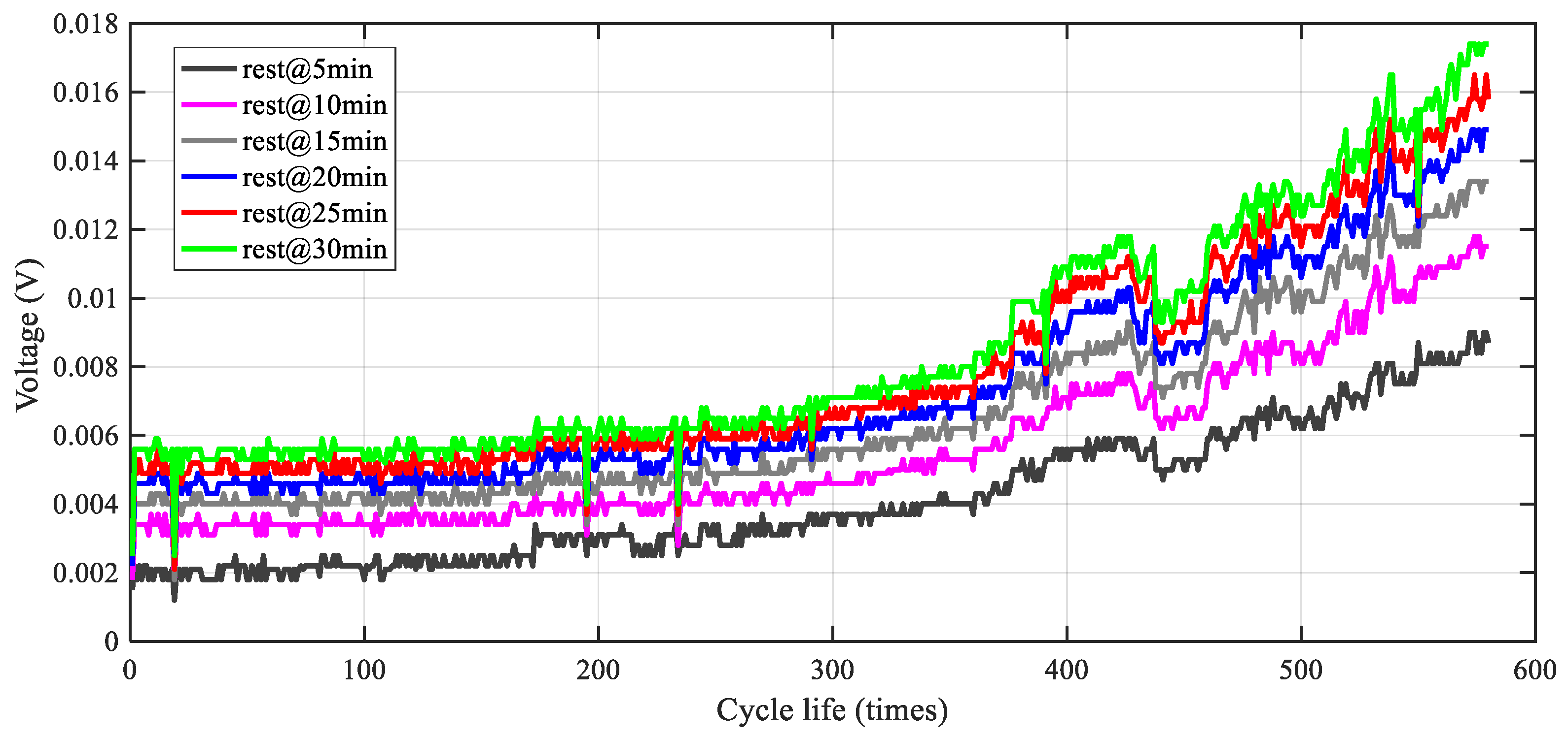
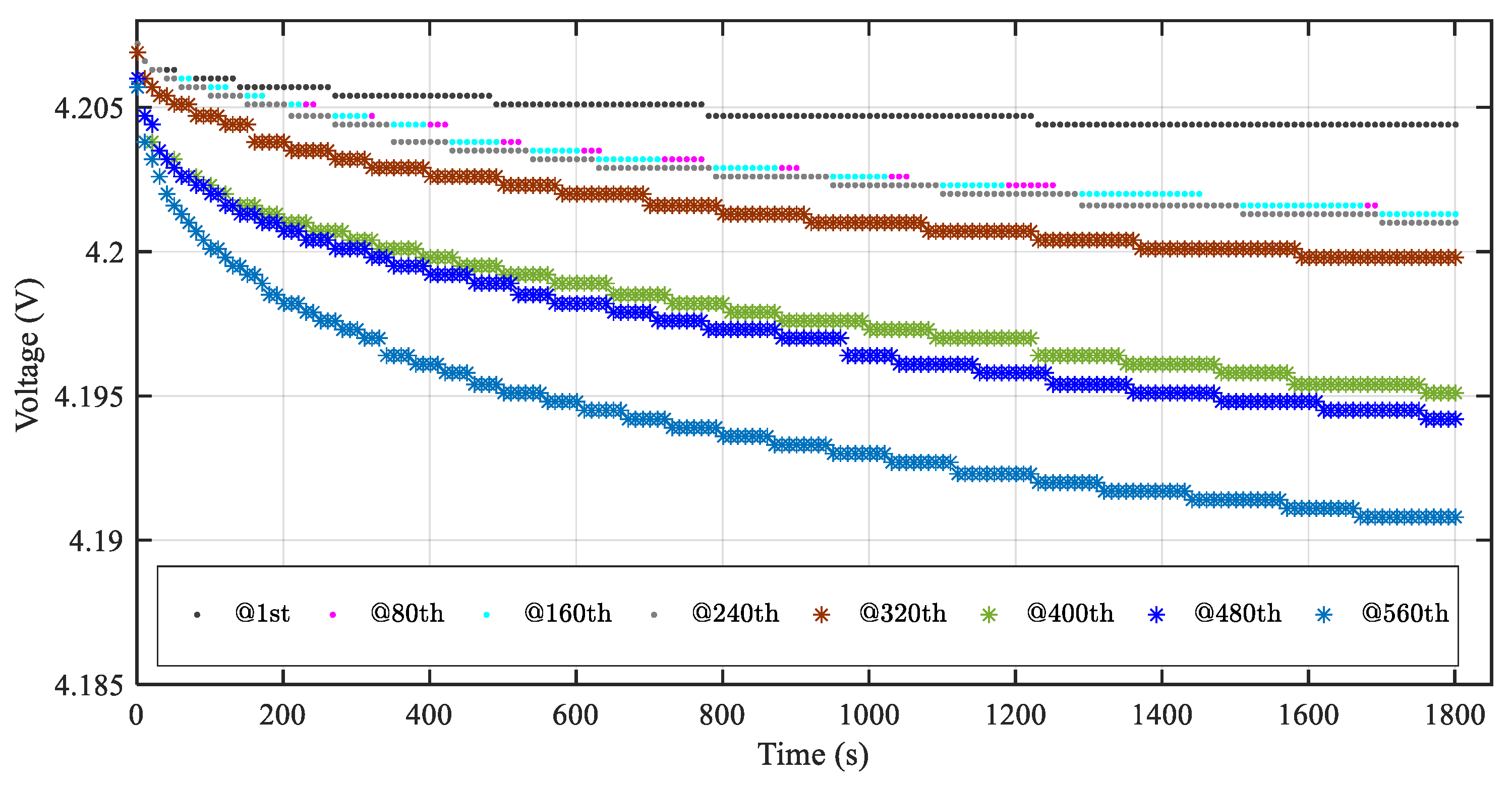
To clarify the relationship between the terminal voltage drop during rest and the degree of degradation of the battery, Figure 7 showed, in each cycle test, when the No. 1 battery was charged to fully charged state under the operation conditions in cycle test, the terminal voltage drop after 5, 10, 15, 20, 25 and 30 min of rest. Figure 8 shows the changes in the terminal voltage drop when the No.1 battery was charged to the fully charged state in the 1st, 80th,…, 560th cycle tests.

Figure 7 and Figure 8 showed that:

(1) The increasing number of battery life cycles, the change in the terminal voltage drop is increasing for the same rest time.

(2) For the same cycle life test, with the increase in resting time, the change in the terminal voltage drop is decreases. For example, the voltage drop of the first 5 minutes is bigger than the voltage drop of the second 5 min.

(3) During the whole rest duration, at the beginning of the rest, the voltage drop is the fastest and with the increase in the number of battery life cycles, the voltage drop gets faster.

4.2. Constructing the Health Factor

In order to reflect the trend of the terminal voltage drop during the resting period after the battery was fully charged, the following features are selected to construct the health factor.

(1) The terminal voltage drop after the battery rests for 5, 10, 15, 20, 25 and 30 min;

(2) The terminal voltage drop when the battery begins to rest, from the 5th to 10th minute, 10th to 15th minute, 15th to 20th minute, 20th to 25th minute and 25th to 30th minute. The reason for choosing these characteristics as the health factor is that, the terminal voltage drop over time is nonlinear and the terminal voltage drop with the aging of the battery is also nonlinear. Choosing different features as the health factor will affect the accuracy of the results.

4.3. Analysis of the SVM

SVM is a machine learning method for classification, regression, or other learning tasks. This analysis is based on structural risk minimization and it can minimize the empirical risk and confidence interval [44,45]. SVM is chosen for the excellent approximation and generalization capability and its demonstrated potential in the realm of nonlinear system identification. A typical SVM application included two steps:

(1) Training the sample set data to obtain a model between the input and output data;

(2) Using the model to predict the test set data.

Supposed the training sample set is $\{(x_1,y_1),\dots ,(x_l,y_l)\}$. In which, $x_i\in R^n$, that is, x_i is an n-dimensional feature vector and $y_i\in R$. l is the sample number.

When SVM is used for regression, its purpose is to get a regression model as Equation (6) to minimize the error between model outputs f(x) and desired values y. $\omega$ and b are the parameters to be determined. Here, $\omega$ is also an n-dimensional feature vector, ${\omega }^T$ denotes the transpose of the vector $\omega$. b is the deviation and it is a scalar.

$$f(x)={\omega }^{T}x+b$$

(6)

It supposes that the maximum deviation between the model output and the desired value we can tolerate is $\epsilon$ (that is, a positive constant). Then, when the estimation error of a sample is less than $\epsilon$, the estimate result of the sample is correct.

According to the principle of structural risk minimization, Equation (7) is used to identify the parameters $\omega$ and b:

$$\underset{\omega ,b}{\min } \frac{1}{2}{\Vert \omega \Vert }^2+C\cdot {\displaystyle \sum _{i=1}^l{\ell }_{\epsilon }(f(x_i)-y_i)}$$

(7)

In which, $\Vert \Vert$ represents the Euclidean norm. C represents the regularization parameter or called penalty factor. The definition ${\ell }_{\epsilon }$ is showed as Equation (8):

$${\ell }_{\epsilon }(z)=\{\begin{array}{ll}0,& \mathrm{if} \left|z\right|\le \epsilon ;\\ \left|z\right|-\epsilon ,& \mathrm{otherwise}.\end{array}$$

(8)

By introducing the non-negative relaxation variables ${\xi }_i$ and ${\xi }_i^{*}$(I = 1, 2,…, l), Equation (7) is equivalent to:

$$\underset{\omega ,b,{\xi }_i,{\xi }_i^{*}}{\min } \frac{1}{2}{\Vert \omega \Vert }^2+C\cdot {\displaystyle \sum _{i=1}^l({\xi }_i+{\xi }_i^{*})}$$

(9)

$$s.t.\{\begin{array}{l}f(x_i)-y_i\le \epsilon +{\xi }_i\\ y_i-f(x_i)\le \epsilon +{\xi }_i^{*}\end{array}$$

By importing the Lagrange multipliers $a_i\ge 0, a_i^{*}\ge 0, u_i\ge 0, u_i^{*}\ge 0$, it can obtain the Lagrangian function of the Equation (9):

$$\begin{array}{l}L(\omega ,b,a,a^{*},\xi ,{\xi }^{*},u,u^{*})\\ =\frac{1}{2}{\Vert \omega \Vert }^2+C\cdot {\displaystyle \sum _{i=1}^l({\xi }_i+{\xi }_i^{*})}-{\displaystyle \sum _{i=1}^l{u}_i{\xi }_i-}{\displaystyle \sum _{i=1}^l{u}_i^{*}{\xi }_i^{*}}\\ +{\displaystyle \sum _{i=1}^l{a}_i(f(x_i)-y_i-\epsilon -{\xi }_i)}+{\displaystyle \sum _{i=1}^l{a}_i^{*}(y_i-f(x_i)-\epsilon -{\xi }_i^{*})}\end{array}$$

(10)

It follows from the saddle point condition of convex programs that the partial derivatives of $L(\omega ,b,a,a^{*},\xi ,{\xi }^{*},u,u^{*})$ with respect to the primal variables $\omega , b, {\xi }_i, {\xi }_i^{*}$ have to vanish for optimality, that is:

$$\omega ={\displaystyle \sum _{i=1}^l(a_i^{*}-a_i)x_i}$$

(11)

$$0={\displaystyle \sum _{i=1}^l(a_i^{*}-a_i)}$$

(12)

$$C=a_i+u_i$$

(13)

$$C=a_i{}^{*}+u_i{}^{*}$$

(14)

Substituting Equations (11)–(14) into (10), yields the dual program:

$$\underset{a,a^{*}}{\max }{\displaystyle \sum _{i=1}^l{y}_i(a_i^{*}-a_i)-\epsilon \cdot (a_i^{*}+a_i)}-\frac{1}{2}\cdot {\displaystyle \sum _{i=1}^l{\displaystyle \sum _{j=1}^l(a_i^{*}-a_i)(a_j^{*}-a_j)x_i^T{x}_j}}$$

(15)

$$\begin{array}{ll}s.t.& {\displaystyle \sum _{i=1}^l(a_i^{*}-a_i)=0 ,}\\ & 0\le a_i , a_i^{*}\le C .\end{array}$$

The above process has to satisfy the Karush-Kuhn-Tucker (KKT) condition, that is:

$$\{\begin{array}{l}{a}_i\cdot (f(x_i)-y_i-\epsilon -{\xi }_i)=0\\ a_i^{*}\cdot (y_i-f(x_i)-\epsilon -{\xi }_i^{*})=0\\ a_i\cdot a_i^{*}=0 , {\xi }_i\cdot {\xi }_i^{*}=0 ,\\ (C-a_i)\cdot {\xi }_i=0 , (C-a_i^{*})\cdot {\xi }_i^{*}=0 .\end{array}$$

(16)

When it gets the solution $a_i$ and $a_i^{*}$ of Equation (15), substituting Equation (11) into (6), it can obtain the following Equation (17):

$$f(x)={\displaystyle \sum _{i=1}^l(a_i^{*}-a_i)x_i^{T}x+b}$$

(17)

Combining the solution $a_i$ and $a_i^{*}$ of Equation (15) with Equation (16), it can get the value of b:

$$b=y_i+\epsilon -{\displaystyle \sum _{j=1}^l(a_j^{*}-a_j)x_j^T{x}_i}$$

(18)

When the linear characteristics of samples are not obvious, the nonlinear mapping function $\varphi (x)$ is adopted to map the low-dimensional feature space $R^n$ to a high-dimensional space H, that is, Hilbert space.

Then, the x will be replaced with $\varphi (x)$ and the regression model (6) becomes the Equation (19):

$$f(x)={\omega }^T\cdot \varphi (x)+b$$

(19)

Consequently, Equation (17) becomes the following equation:

$$\omega ={\displaystyle \sum _{i=1}^l(a_i^{*}-a_i)\varphi (x_i)}$$

(20)

Then the regression model (19) can be represented as:

$$f(x)={\displaystyle \sum _{i=1}^l(a_i^{*}-a_i)k(x,x_i)+b}$$

(21)

In which, $k(x_i,x_j)=\varphi {(x_i)}^T\cdot \varphi (x_j)$. It is a kernel function. Common kernel functions of the SVM are the linear kernel function, polynomial kernel function, radial basis kernel function (RBF) and two-layer perceptive kernel function. In this paper, we use the RBF, as shown in Equation (22):

$$k(x_i,x)=\exp (-g{\Vert x-x_i\Vert }^2),g>0$$

(22)

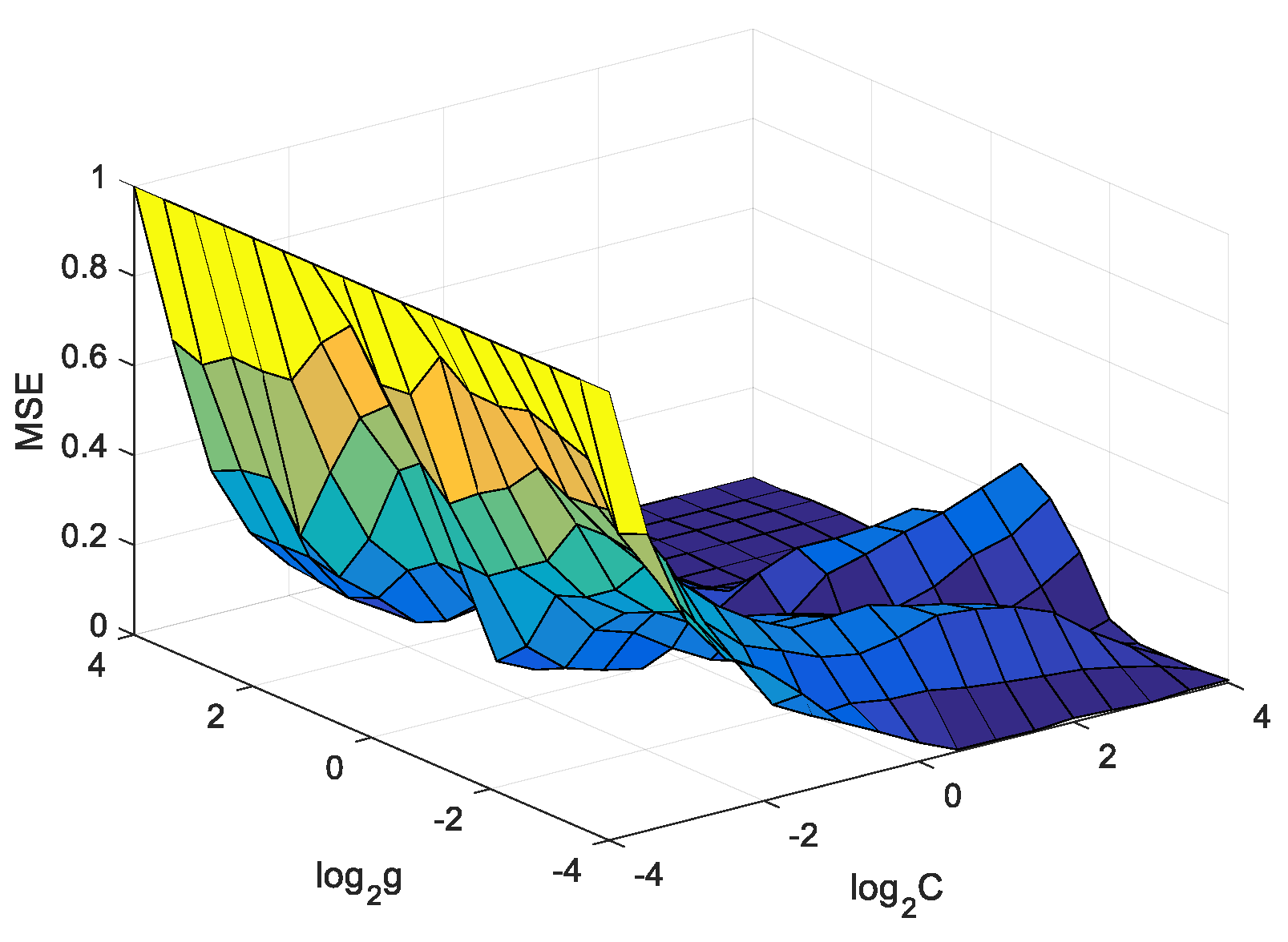
Prior to the SVM training, the penalty factor C and kernel function parameters g need to be predetermined.

About the detailed solution process of SVM and the information on kernel function, please refer to the references [46].

4.4. Available Capacity Prediction Model of Battery Based on the SVM

The steps of available capacity estimation modeling based on the SVM are as follows:

Step 1: For the cycle life test of the No. 1 battery, obtain the health factors according to the method of Section 4.2 and adopt it as input $x_i$ and adopt the discharging capacity as output $y_i$.

Step 2: Normalize the input and output data;

Step 3: Use the cross-validation method to select the optimal parameters C and $g$ of the regression;

Step 4: Use the optimal parameters obtained in Step 3 to train the SVM and get the model.

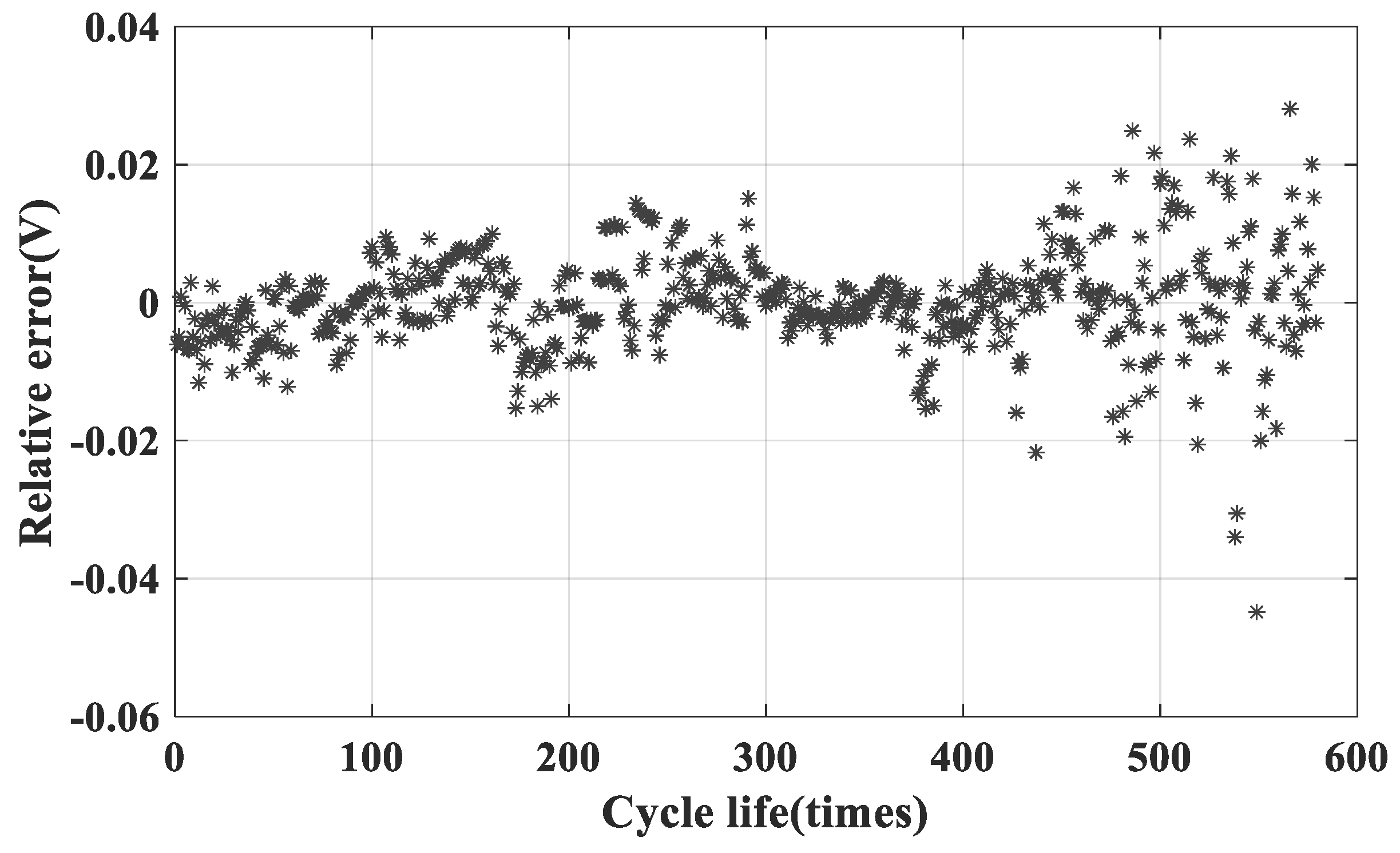
The model is used to estimate the available capacity and the corresponding SOH. The following Equations (23)–(25) are used to calculate the performance indices, included the mean squared error (MSE), squared correlation coefficient R² and relative error Error.

$$MSE=\frac{1}{l}{\displaystyle \sum _{i=1}^l{(f(x_i)-y_i)}^2}$$

(23)

$$R^2=\frac{{(l{\displaystyle {\sum }_{i=1}^{l}f(x_i)y_i-{\displaystyle {\sum }_{i=1}^{l}f(x_i){\displaystyle {\sum }_{i=1}^l{y}_i}}})}^2}{(l{{\displaystyle {\sum }_{i=1}^{l}f(x_i)}}^2-{({\displaystyle {\sum }_{i=1}^{l}f(x_i)})}^2)(l{\displaystyle {\sum }_{i=1}^l{y}_i^2-{({\displaystyle {\sum }_{i=1}^l{y}_i})}^2})}$$

(24)

$$Erro{r}_i=\frac{\left|f(x_i)-y_i\right|}{y_i}$$

(25)

In Equations (23)–(25), l represents the total number tests, f represents the estimated available capacity of the ith test, i.e., the ith health factor and, y_i represents the real available capacity of the battery.

5. Experimental Results and Discussion

This section verified the performance of the model connecting health factor and available capacity of the battery. The model is established by a SVM approach. The validation will be performed on the following three aspects:

(1) The health factor containing the feature extracted from the terminal voltage drop is meaningful;

(2) The health factor is able to reflect the SOH of the battery. The battery using such health factor is not constrained by the working condition. In addition, the results of the paper are compared with the results based on OCV method;

(3) The model can be used for other battery with the same type. The method proposed is reasonable.

5.1. Verification of the Health Factor

Table 2. Features of the health factor.

Feature Name	Feature Description
No.1	Rest for 5 min
No.2	Rest for 10 min
No.3	Rest for 15 min
No.4	Rest for 20 min
No.5	Rest for 25 min
No.6	Rest for 30 min
No.7	5–10 min duration
No.8	10–15 min duration
No.9	15–20 min duration
No.10	20–25 min duration
No.11	25–30 min duration

showed the features that are used to construct the health factor. “Rest for x min” represents the value of the terminal voltage drop after the fully charged battery has rested for x min. “y–z min duration” represents the terminal voltage drop from the yth minute to the zth minute during the fully charged battery’s rest.

Using these different features as health factors to establish SVM model, it will obtain different MSEs, R2 values and average relative errors. The results are shown in

Table 3. performance parameters.

Feature	12	1	1-2	1-3	1-4	1-5
MSE	0.00174481	0.0017128	0.00129276	0.0011000	0.00100485	0.0009935
R2	97.2716%	97.2993%	97.9575%	98.2644%	98.4136%	98.4372%
Average Error	0.6687%	0.7232%	0.6027%	0.5465%	0.5281%	0.5239%
Feature	1–6	1–7	1–8	1–9	1–10	1–11
MSE	0.00098901	0.00091085	0.00091220	0.00092457	0.000947030	0.0008561
R2	98.4447%	98.5616%	98.5604%	98.5408%	98.5044%	98.6481%
Average Error	0.5239%	0.5048%	0.4984%	0.5083%	0.5112%	0.4881%

. Feature 1 represents using the No. 1 feature of Table 2 as the health factor, “1–x” represents using all the features from the No. 1 feature to the No. x feature of Table 2 to construct the health factor. Feature 12 represents adopting the terminal voltage drop of the battery when it has rested for 30 min after being fully charged as the health factor.

Table 3 showed that if only the terminal voltage drop after 30 min is selected as the feature of the health factor, the MSE and average error are relatively large. The MSE and average error are reduced and the R² decreases gradually with an increasing number of features. Table 3 presented that using Features 1–11 can get the best estimation result. Features 1–11 is used to construct the health factor and to establish the SVM model in the following estimation and validation tests.

5.2. Estimation Results and Discussion

5.2.1. Estimation Results of SVM

Figure 9 showed the results of using the cross-validation method to select the optimal parameters C and $g$. Figure 10 showed the estimation result of the test data set and Figure 11 presented the relative error of the estimation result.

Table 4. Relative error statistics.

Relative error Interval	Minimum	Maximum	Number of Times
Error < 1%	9.992e-06	0.0099	518
1% < Error < 2%	0.0101	0.0190	56
2% < Error < 3%	0.0207	0.0299	5
3% < Error < 4%	0	0	0
4% < Error < 5%	0.0411	0.0411	1
5% < Error < 6%	0	0	0

indicated the statistical results of the relative error and showed the result in Figure 11.

The following tests are carried out in order to verify that the algorithm is less dependent of the working conditions. As mentioned in Section 3.2, an OCV experiment is carried out after 80–100 cycle life tests. In each OCV test, before discharging the battery, the battery is charged to the fully charged state and rests for 30 min, just like in the cycle life test and then the health factor of the battery is obtained in this OCV test. An available capacity of the battery corresponding to the health factor can be obtained using this health factor as an input of the SVM model. The battery life decay is a slow process in real applications, the measured available capacity in the last cycle life test before the OCV test is adopted as the real available capacity. The estimated available capacity of the SVM model and the real available capacity are compared. The SOH and the estimated relative results are showed in

Table 5. Estimated error of No. 1 battery in test 2.

Cycle Number	Real Available Capacity (mAH)	Estimated Available Capacity (mAH)	Real SOH	Estimated SOH	Relative Error
1	1495.3	1489.052	99.69%	99.27%	0.42%
100	1486.2	1474.655	99.08%	98.31%	0.78%
195	1458.4	1455.447	97.23%	97.03%	0.21%
293	1412.3	1421.132	94.74%	95.04%	0.62%
392	1365.9	1361.420	91.06%	90.76%	0.33%
553	1267.3	1249.908	84.49%	83.33%	1.39%

.

5.2.2. Results Analysis of SVM

The experimental results are analyzed.

(1) The statistical relative error in Figure 8 shows that, compared to the relative error in the early and middle cycles, the relative error in the later cycles is relatively large. The main reason lies in the fact that, when the life of the LIB is about to reach its end, the capacity deterioration is aggravated. Even if there is a short-term capacity recovery, it decreases rapidly for relatively short life cycles.

(2) The total number of cycle life tests is 580. A total of 518 estimation errors (i.e., 89.31%) are less than 1%, a total of 574 estimation errors (i.e., 98.97%) are less than 2% and only one relative error is more than 3%, accounting for 0.17% of the total.

(3) Considered the fact that using the health factor only containing the feature extracted from the terminal voltage drop during the battery having a rest to predict the capacity and SOH of the battery, for the health factor has less dependent on the working condition, the predict result has high robustness to the working conditions. Table 5 showed the proposed method gets high precision under different working conditions.

Therefore, according to the relative error statistics, it is feasible to estimate the available capacity and SOH of a LIB using the information on the terminal voltage drop when the full charged battery is resting.

5.2.3. Estimation Results of OCV

Using OCV experimental data, the available capacity data of lithium-ion batteries can be obtained by using the method based on OCV method, the flowchart of this method [16] is illustrated in Figure 12.

The following processing is carried out to fully explain the characteristics of OCV based method:

(1) Using the discharging data to estimate the capacity of the battery;

(2) Fitting the OCV-SOC curve according to the first OCV experimental data. Polynomial fitting method was adopted and the order of polynomials is 5, 8 and 11 orders respectively;

(3) Six SOC intervals including 100%–35%, 95%–30%, 95%–25%, 90%-35%, 90%–25% and 90%-50% are used to estimate the available capacity of the battery. Figure 13 presented the results.

5.2.4. Results Analysis of OCV

Figure 13 showed that the SOC interval and the OCV-SOC curve influence the capacity estimation result.

(1) The SOC value is calculated on the basis of OCV value, thus the accuracy of the OCV-SOC curve will affect the prediction result. Figure 13 shows that the estimation errors of different OCV-SOC curves are different;

(2) The OCV test will obtain multiple corresponding points of OCV value and SOC value and these corresponding points are used to fit the OCV-SOC curve. In generally, the errors between the fitting value and the real value of the two ends of the fitting curve are relative larger. The above SOC interval 1 (100%–35%) has a large error due to use the 100% SOC value. For SOC interval 3 (95%–25%) and SOC interval 5 (90%–25%), the lower SOC of these two intervals is 25%, with the degradation of the battery, this 25% SOC will reduce to a relative small value. For example, if the nominal capacity of the battery is 1500 mAh, when the fresh battery with full charged is discharged for 1125 mAh, then the SOC is changed from 100% to 25%. However, when the fresh battery degenerates into an old one and its life will end; its available capacity is degraded into 1200 mAh, if the battery with full charged is still discharged for 1125 mAh, then the SOC is changed from 100% to 6.25% which is below 10% and the OCV-SOC fitting error is larger. Figure 13 showed, in the later battery life, the estimating error is larger for the two SOC intervals than the error in the early battery life;

(3) The SOC interval is greater than 60%, the estimation results are more accurate [18]. The SOC interval 4 (90%–35%) and the SOC interval 6 (90%–50%) are less than 60%. Figure 13 indicated the estimate error of such two SOC interval are relative larger for the three OCV-SOC curve with different orders.

In summary, the SOC interval 2 (95%–30%) not only satisfies that the SOC interval is more than 60% but also satisfies that the 100% SOC and the SOC below 10% are not used. Form Figure 13, it can be seen that the estimating errors using such SOC interval are relative small and the estimate error of the OCV-SOC curve with 11 order polynomial is the smallest.

5.2.5. Comparison Analysis the Method Based on OCV and the Method of This Study

In all above 18 estimations, the one with SOC interval 95%–30% and 11 order polynomial OCV-SOC curve has the smallest estimated error, which is showed in

Table 6. Estimated error of method based on OCV.

Cycle Number	Real Available Capacity (mAH)	Estimated Available Capacity (mAH)	Real SOH	Estimated SOH	Relative Error
1	1495.3	1486.91	99.69%	99.13%	0.56%
100	1486.2	1473.59	99.08%	98.24%	0.85%
195	1458.4	1450.04	97.23%	96.67%	0.57%
293	1412.3	1430.27	94.15%	95.35%	1.27%
392	1365.9	1394.54	91.06%	92.97%	2.10%
553	1267.3	1308.15	84.49%	87.21%	3.22%

.

Compared the Table 6 with Table 5, first of all, just like SOH prediction method proposed, in the early and middle cycles, the relative error of the method based on OCV is smaller than it in the later cycles. And, the relative error of the method proposed is smaller than that of method based on OCV. The OCV-SOC curve is affected by the aging of the battery. In other words, the real OCV-SOC relationship is related to the working condition and the degradation of the battery. Therefore, only using the OCV-SOC curve obtained only according to the first OCV test is lack of precision. The influence of hysteresis effect is becoming increasingly with the degradation of the battery; therefore, in the later cycles of the battery, the estimating errors are bigger than those of in the early or middle cycles.

5.3. Validation and Analysis of Effectiveness

The No. 2 battery is used to test the model trained by the SVM to verify that the algorithm is not an accidental result but is suitable for this type of LIB. The health factor and the corresponding discharge capacity (the available capacity) of the No. 2 battery are used as the test data set to test the SVM model of the No. 1 battery and the error results are shown in

Table 7. Estimated error of No.2 battery in test 1.

Cycle Number	Real Available Capacity (mAH)	Estimated Available Capacity (mAH)	Real SOH	Estimated SOH	Relative Error
60	1492.8	1497.524	99.52%	99.83%	0.31%
120	1473.8	1468.611	98.25%	97.91%	0.35%
180	1453.7	1482.828	96.91%	98.86%	2.00%
240	1429.9	1442.154	95.33%	96.14%	0.85%
300	1407.4	1446.934	93.83%	96.46%	2.81%
360	1400.7	1421.848	93.38%	94.79%	1.49%
420	1353.6	1369.674	90.24%	91.31%	1.19%
480	1318.8	1325.427	87.92%	88.36%	0.50%
540	1238.4	1247.826	82.56%	83.19%	0.76%

. The OCV test information about the No. 2 battery is used to test the model shown in

Table 8. Estimated error of No. 2 battery in test 2.

Cycle Number	Real Available Capacity (mAH)	Estimated Available Capacity (mAH)	Real SOH	Estimated SOH	Relative Error
1	1487.9	1500.000	99.19%	100%	0.81%
100	1480.6	1467.195	98.71%	97.81%	0.91%
195	1451.4	1472.828	96.76%	98.19%	1.45%
293	1400.9	1423.009	93.39%	94.87%	1.58%
392	1365.1	1376.083	91.01%	91.74%	0.80%
553	1226.2	1239.048	81.75%	82.60%	1.04%

. The meaning of each parameter in Table 8 is same as the corresponding parameter in Table 5.

Table 7 and Table 8 presented that when the trained SVM model of the No. 1 battery is used to estimate the available capacity and SOH of the No. 2 battery, the relative error of the No. 2 battery is bigger than that of the No. 1 battery; most of the estimated relative errors are within 2% and the maximum relative error is less than 3%. The results also indicate that the model built using the No. 1 battery can be used for all batteries of the same type. In other words, it is feasible to use the terminal voltage drop information to estimate the available capacity and SOH. It is important to note that, due to the inherent inconsistencies of the batteries, there are some differences even for the same type of battery. These differences can explain why the overall estimation error of the No. 2 battery is larger than that of the No. 1 battery.

6. Conclusions

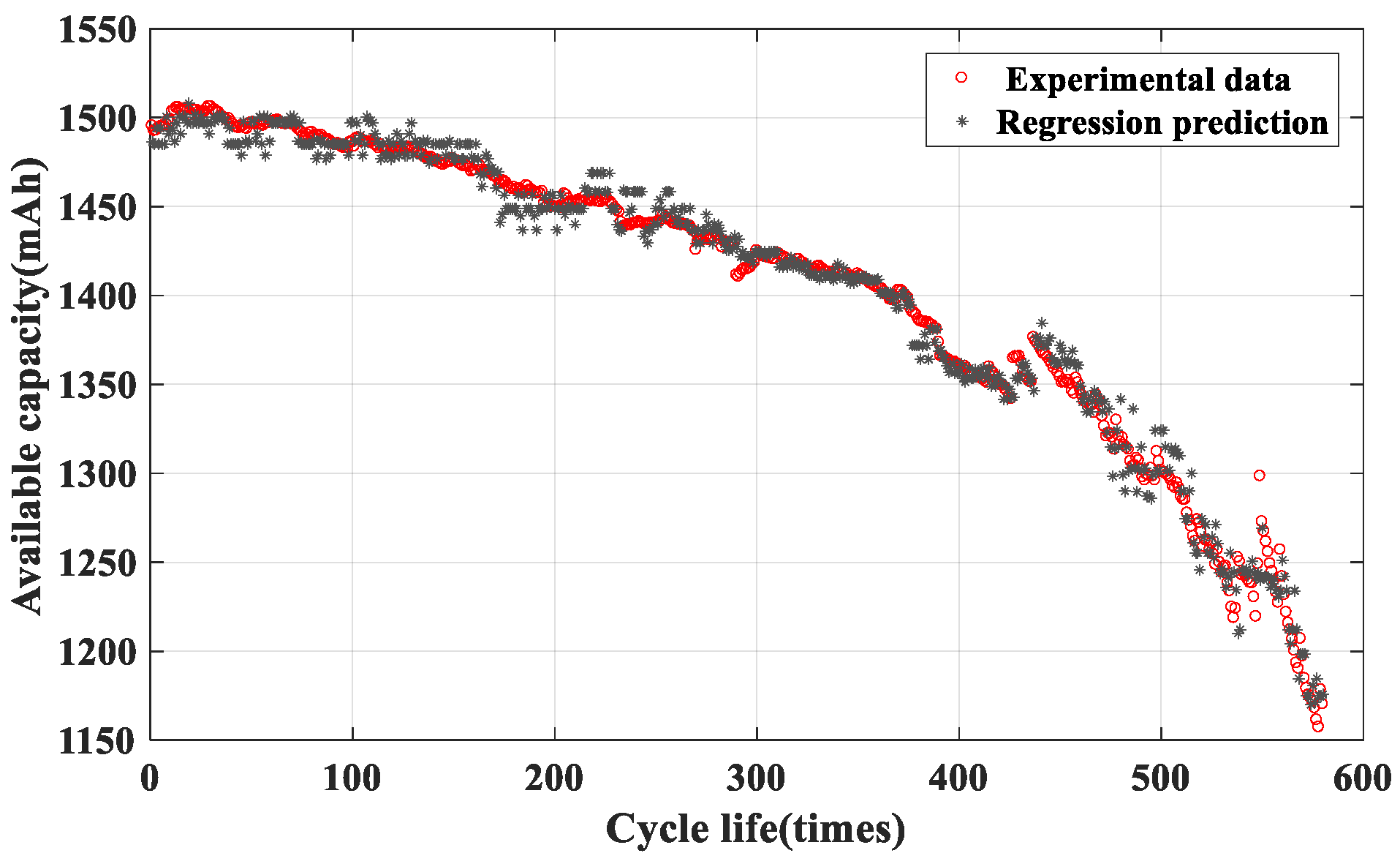
The SOH is an important index to measure battery performance and is also a hot topic in LIB research for the renewable energy industry. Combining the cycle life test data and OCV characteristics, a novel SOH method is proposed by analyzed the current SOH prediction method. This study makes use of the information on the terminal voltage drop when the battery is resting after it has been charged to a given voltage as the health factor. This study adopts the SVM to obtain the relationship between the health factor and the available capacity. Two batteries of the same type were used, one is for SVM modelling and the other is for verifying. The results show that, using the model built in this paper to predict the available capacity and SOH of the battery, almost all of the relative errors are within 3%; as a consequence, the proposed method is feasible.

The reason why it is difficult to charge or discharge a battery to a certain exact SOC is analyzed in detail. or it only uses features extracted from the terminal voltage drop during the battery rest to obtain the health factor, the health factor is less dependent on the working condition.

In addition, the experiments of the paper are implemented at room temperature. The level of the terminal voltage drop during the battery rest may be affected by environmental conditions including temperature and humidity. Qualitative and quantitative analysis of such effect will be carried out in future work.