Head-Raising of Snake Robots Based on a Predefined Spiral Curve Method

Abstract

A snake robot has to raise its head to acquire a wide visual space for planning complex tasks such as inspecting unknown environments, tracking a flying object and acting as a manipulator with its raising part. However, only a few researchers currently focus on analyzing the head-raising motion of snake robots. Thus, a predefined spiral curve method is proposed for the head-raising motion of such robots. First, the expression of the predefined spiral curve is designed. Second, with the curve and a line segments model of a snake robot, a shape-fitting algorithm is developed for constraining the robot’s macro shape. Third, the coordinate system of the line segments model of the robot is established. Then, phase-shifting and angle-solving algorithms are developed to obtain the angle sequences of roll, pitch, and yaw during the head-raising motion. Finally, the head-raising motion is simulated using the angle sequences to validate the feasibility of this method.

1. Introduction

A snake robot is a mobile robot with a long and slender body and plays a crucial role in search and rescue operations, inspection and maintenance [1]. Controlling such robots is difficult, and a review of their modeling, implementation, and control can be found in [2]. Generally, for given tasks such as searching a trapped person in disaster areas, tracking a flying object and repairing a damaged pipe as a manipulator, the snake robot has to move its body with different motion modes, and head-raising motion is one of them. Snake robots’ common motion modes include serpentine [3,4], traveling wave [5,6], concertina [7,8], and sidewinding [9,10] locomotion. Additionally, some researchers sought to find other motion modes such as fusion gait [11] and obstacle-aided locomotion [12]. However, these motion modes provide limited visual information. Consequently, snake robots have to raise their heads to observe their surroundings and perform their tasks. Therefore, the motion planning for head-raising of a snake robot is our research object in this paper.

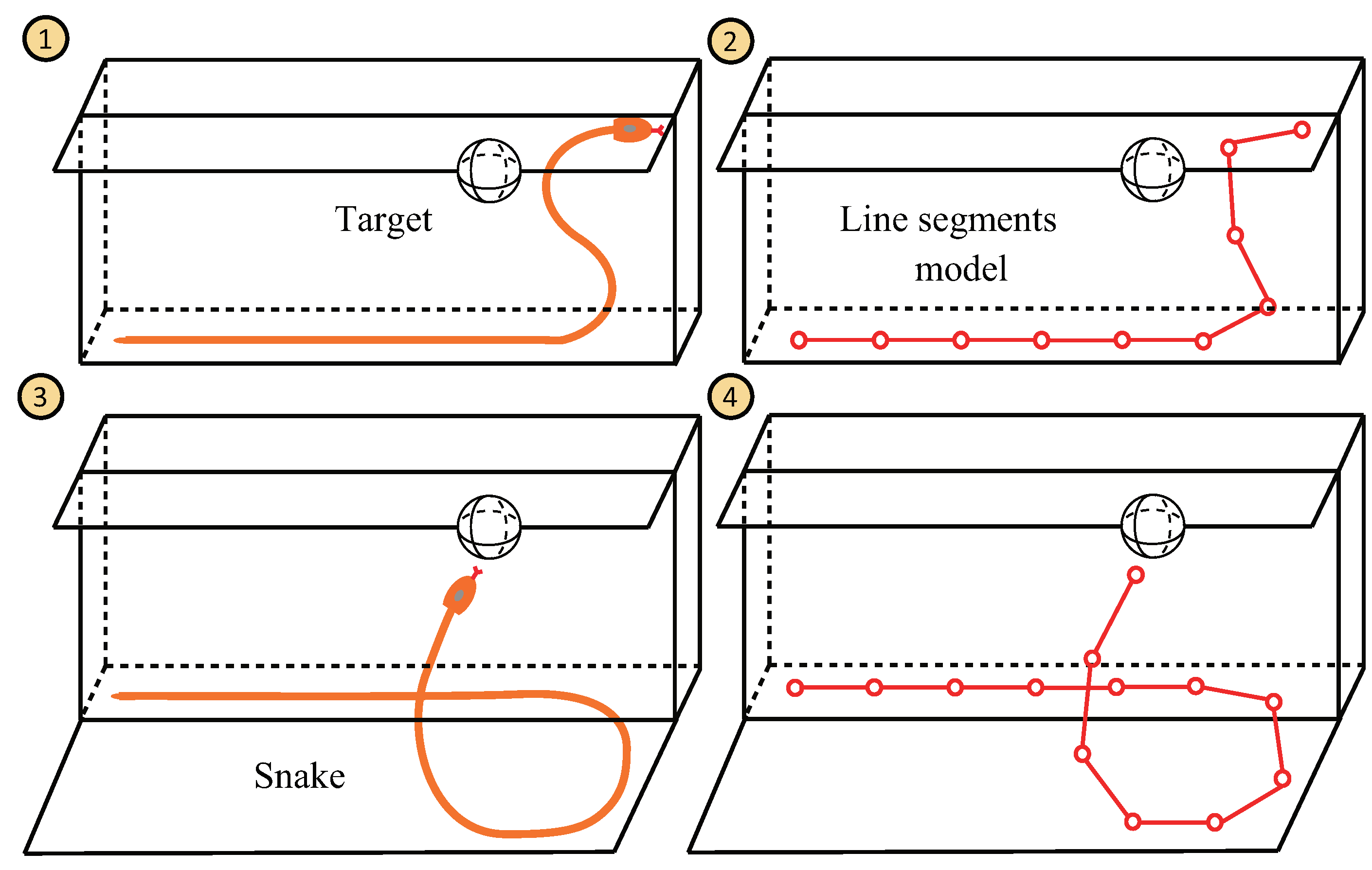
To the best of our knowledge, a few researches on head-raising motion of snake robots have been done, and they can be divided into two types: 2D (two dimensional) head-raising and 3D (three-dimensional) head-raising. This study aims at 3D head-raising. The concepts of 2D and 3D head-raising are illustrated in Figure 1. It should be noted that label 2 and 4 are line segments models of snake robots, which will be utilized in subsequent chapters for simulations. 2D head-raising can be found in [13], the authors proposed an improving serpentine input function to achieve the head-raising motion of a snake robot and analyzed the zero-moment point to assess the stability of the robot. As for 3D head-raising [14,15], to realize it is more complicated. In [14], the works were based on an assumption that the head part of the robot is not contact with the ground and regarded as a manipulator, which is able to achieve several sub-tasks in 3D environment. Therefore, essentially speaking, the researchers mainly considered tracking the trajectory of a snake robot’s head rather than the head-raising process. Inspired by the work made by Tanka et al, we currently are working on trajectory tracking of the snake robot head by improving our model. There still exists problems to be solved and a video about the trajectory tracking (Concept_of_trajectory_tracking.avi) can be seen in Supplementary Materials. In [15], the authors regarded a snake robot as a serially linked floating-base robot and divided it into base and active modules. The base modules were used to construct the support polygon for maintaining stability during the head-raising process and can be changed to active modules to allow the head to stretch to a given position and orientation. The trajectory functions of individual joints were set as parameterized cubic spline curves, and the head-raising motion was achieved by optimizing these parameters according to some criterions. In summary, existing works of head-raising attempt to find the input functions of individual joints. However, in this study, the input functions (angle sequences with respect to time) are unknown, and they are obtained by shape-fitting and phase-shifting algorithms, which will be introduced in the subsequent chapters.

Achieving motion control for a snake robot is difficult because of the kinematic redundancy, which can be solved by the shape control method. Motion control based on a spiral curve belongs to the category of the shape control. It is necessary to introduce the concept of shape control method. This method can not be described in theory, and it is a kind of idea to control the motion of snake robots or hyper-redundant manipulators. The idea of shape control method is employing a geometric curve to constrain a robot’s configuration by fitting the continuous curve and discrete link model as closely as possible. If change the shape of the geometric curve with respect to time, the robot can achieve continuous motion. The key points to use this method include two aspects. First, how to find a proper curve to describe the shape of robots should be considered. Second, if the curve is obtained, there should be an approach to accomplish the fitting process. Examples of using shape control method can be found in [16,17,18,19,20,21,22,23,24,25]. In [16], the authors presented a geometric spline method for the shape control of planar manipulators with hyper-degrees of freedom. With the fitting of the robotic macro configuration and the referent spline curve, real-time control could be easily accomplished. In [17], the authors presented locomotion control using a phase oscillator network, which can produce a smooth transition of the body shape of a snake robot to avoid obstacles. In [18], the researchers introduced a framework to control the shape of robots, and the framework can be divided into four steps, namely, defining the shape control point, using the shape control point to define the Bezier curves, fitting the curves and the shape of the robot, and changing the parameters of the Bezier curves to control the movement of the snake robot according to the desired gait. In [19], the authors used the shape control point method to control the position and orientation of the head of a robot. In [20], the researchers presented a planar manipulator that moves according to a variable-structure polygon function produced by neural networks. In [21], the authors introduced and used a modal approach to generate a backbone curve and thus capture a hyper-redundant manipulator’s macroscopic geometric feature. The backbone curve was represented by the linear combination of a set of shape functions with the appropriate coefficients. Then, inverse kinematics reduced to the solution of these coefficients to avoid the heavy computation required by the Jacobian pseudo-inverse method. In [22], the researchers analyzed the curvature of the sidewinding locomotion of a snake robot and developed algorithms to fit the robot’s shape to a continuous curve. In [23], the authors proposed the annealed chain fitting algorithm and keyframe wave extraction algorithm; the former maps the shape of the snake robot to a continuous backbone curve and obtains a set of joint angles, whereas the latter obtains a sequence of backbone curves. A similar modeling strategy can also be found in [24,25]. In [25], the researchers considered dynamics during the shape control of hyper-redundant manipulators.

The goal of this paper is to propose a new approach to raise a snake robot’s head in 3D environments. This mechanism allows the robot to obtain a ${360}^{\circ }$ field of view and a large working space. In this paper, inspired by the shape control method, a head-raising motion control method based on a predefined spiral curve is proposed. The robot is represented by several line segments, and the corresponding local coordinate system is established. Every line segment corresponds to a module of the snake robot, and the connection point between adjacent line segments corresponds to a joint involving three degrees of freedom, namely, roll, pitch, and yaw angles, which can be obtained by matrix transformation of the local coordinate system. The predefined curve is introduced to constrain the macro shape of the snake robot, and a phase-shifting algorithm is developed to drive the snake robot along the curve. During the phase-shifting process, the angle trajectories for the head-raising motion in a given time can be obtained. With the angle trajectories, the head-raising motion can be achieved. The contributions of this work are summarized by following remarks:

• A new shape control curve, the predefined spiral curve, is proposed and it is utilized for 3D head-raising of a snake robot;
• A shape-fitting algorithm is developed for adhering the line segments model of the snake robot to the predefined spiral curve;
• Establishment rules of coordinate system are given for line segments model of the snake robot;
• A phase-shifting and an angle-solving algorithms are presented for obtaining angle trajectories used during head-raising motion.

The remainder of this paper is organized as follows. Section 1 reviews previous researches, analyses the necessity for head-raising and introduces our aim, which is raising a snake robot’s head based on a predefined spiral curve in 3D environments. Section 2 introduces the modeling of the head-raising motion; the mathematical expression of the predefined spiral curve is discussed in SubSection 2.1, the shape-fitting and phase-shifting methods in SubSection 2.2, and the establishment of the coordinate system and angle-solving algorithm in SubSection 2.3. Section 3 explains the simulation of the head-raising motion. Section 4 presents the conclusions.

2. Modeling of Head-Raising Motion

In this section, a predefined spiral curve and a shape-fitting method are introduced to constrain the macro shape of the snake robot, which is composed of serial links represented by serial line segments. However, the serial line segments do not contain the complete information of the snake robot. Therefore, coordinate system is introduced. The snake robot has to move through the predefined spiral curve from initial posture to final posture, and that process is called phase-shifting. With the proposed phase-shifting and angle-solving algorithms, the angle sequences (or angle trajectories) can be used to accomplish the head-raising motion.

2.1. Predefined Spiral Curve

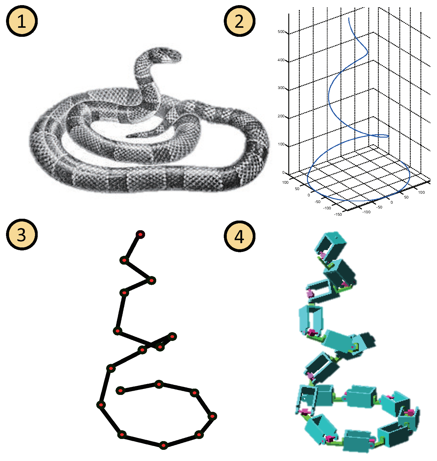
From the biological perspective, a snake’s head-raising movement is irregular, and it is difficult to completely describe its shape using a mathematical model. Based on our observations, the shape of a snake after raising its head is similar to that of a spiral curve, as described in Figure 2. In addition, the spiral curve can ensure the stability of head-raising. Thus, describing the head-raising movement of a snake robot with a spiral curve is reasonable.

$$\begin{array}{c}{x}_s(t)=atsin(t+{\phi }_0)\hfill \\ y_s(t)=atcos(t+{\phi }_0)\hfill \\ z_s(t)=ct\hfill \end{array}$$

(1)

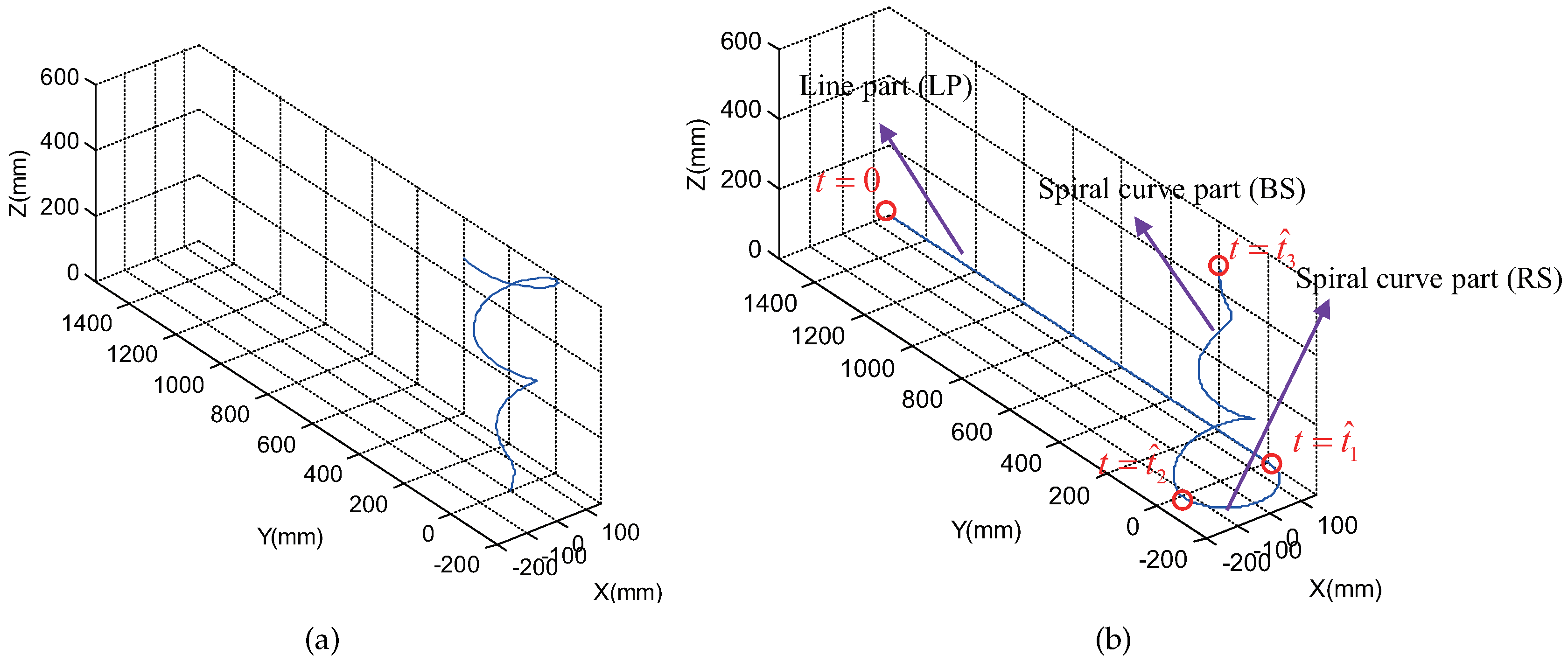
A regular spiral curve (Figure 3a) can be expressed as Equation (1). It cannot be utilized to guide the movement of the robot, and has to be modified, because it cannot ensure the stability of head-raising. Then, the predefined spiral curve (Figure 3b) is designed and its mathematical description satisfies Equation (2), where $x_l(t)$, $y_l(t)$, and $z_l(t)$ represent the line part; $x_s(t)$, $y_s(t)$, and $z_s(t)$ describe the spiral curve part; and a, b, and c are the adjustment coefficients of the spiral curve. The amplitudes of $x_s(t)$ and $y_s(t)$ change equally when a is changed and unequally when b is changed. The amplitude of $z_s(t)$ is influenced by c. ${\phi }_0$ is the initial phase of the sine and cosine functions, which correspond to the slope of the tangent vector for the initial point. $n_c$ is the cycle number of the spiral curve. $l_{link}$ and n are the length and number of the snake robot modules, respectively. t is the independent variable divided into three intervals, which correspond to the line part (defined by LP, interval is $(0,{\widehat{t}}_1)$); the base of the spiral curve part, which is in contact with the ground (defined by BS, interval is $({\widehat{t}}_1,{\widehat{t}}_2)$); and the rest of the spiral curve (defined by RS, interval is $({\widehat{t}}_2,{\widehat{t}}_3)$). ${\phi }_{base}$ is the phase value of the second interval.

$$\begin{array}{c}{x}_l(t)=x_s({\widehat{t}}_1)t\in (0,{\widehat{t}}_1)\hfill \\ y_l(t)=y_s({\widehat{t}}_1)-t+{\widehat{t}}_{1}t\in (0,{\widehat{t}}_1)\hfill \\ z_l(t)=0t\in (0,{\widehat{t}}_1)\hfill \\ x_s(t)=ab({\widehat{t}}_3-t)sin(t+{\phi }_0)t\in ({\widehat{t}}_1,{\widehat{t}}_2)\hfill \\ y_s(t)=a({\widehat{t}}_3-t)cos{(t+{\phi }_0)}_{1}t\in ({\widehat{t}}_1,t_2)\hfill \\ z_s(t)=0t\in ({\widehat{t}}_1,{\widehat{t}}_2)\hfill \\ x_s(t)=ab({\widehat{t}}_3-t)sin(t+{\phi }_0)t\in ({\widehat{t}}_2,{\widehat{t}}_3)\hfill \\ y_s(t)=a({\widehat{t}}_3-t)cos(t+{\phi }_0)t\in ({\widehat{t}}_2,{\widehat{t}}_3)\hfill \\ z_s(t)=ct-c{\widehat{t}}_{2}t\in ({\widehat{t}}_2,{\widehat{t}}_3)\hfill \\ {\widehat{t}}_1=n{l}_{link}\hfill \\ {\widehat{t}}_2={\widehat{t}}_1+{\phi }_{base}\hfill \\ {\widehat{t}}_3={\widehat{t}}_1+2n_c\pi \hfill \end{array}$$

(2)

The predefined spiral curve is composed of a line part and a spiral curve part, as shown in Figure 3b. The line and spiral curve parts constrain the initial and final head-raising postures of the snake robot, respectively. As shown in Figure 3, compared with the regular spiral curve expressed in Equation (1), the predefined spiral curve expressed in Equation (2) introduces parameter b to ensure that $x_s(t)$ and $y_s(t)$ change unequally, interval $(0,{\widehat{t}}_1)$ to construct LP, $({\widehat{t}}_1,{\widehat{t}}_2)$ to construct BS, and $({\widehat{t}}_2,{\widehat{t}}_3)$ to construct RS. Additionally, by substituting item $({\widehat{t}}_3-t)$ for t, it can be ensured that $x_s(t)$ and $y_s(t)$ decrease as $z_s(t)$ increases. Obviously, the predefined spiral curve is appropriate for ensuring stability during head-raising.

2.2. Shape-Fitting and Phase-Shifting Methods

In this section, a shape-fitting and phase-shifting algorithms are developed, and the former ensures that the snake robot adhere to the predefined spiral curve and the latter drive the robot move along with the curve. Figure 4 shows the concepts of these methods. In Figure 4, two links of robot are shown; the red one represents the robot posture at time $t_i$ and the black one corresponds to the robot posture at time $t_{i+1}$. The robot moves from posture at time $t_i$ to posture at time $t_{i+1}$, and this process is called phase-shifting. Two links contain three points; that is, the length between adjacent points equals the length of the robot links. Therefore, the snake links are calculated by point sets and represented by line segments. This process is called shape-fitting.

The details of how the shape-fitting and phase-shifting algorithms work are described in the following steps.

Step 1: Initialization

The parameters a, b, c, $n_c$, n, $l_{link}$, ${\widehat{t}}_1$, ${\widehat{t}}_2$, ${\widehat{t}}_3$, ${\phi }_0$, and ${\phi }_{base}$ are initialized. The following constraint equation is used to ensure that line segments model of the robot do not get away from the ground.

$$\begin{array}{c}{S}_1+S_2=\underset{t={\widehat{t}}_1}{\overset{t={\widehat{t}}_2}{\int }}\sqrt{{\dot{x}}_s{(t)}^2+{\dot{y}}_s{(t)}^2+{\dot{z}}_s{(t)}^2}dt+\hfill \\ \underset{t={\widehat{t}}_2}{\overset{t={\widehat{t}}_3}{\int }}\sqrt{{\dot{x}}_s{(t)}^2+{\dot{y}}_s{(t)}^2+{\dot{z}}_s{(t)}^2}dt<n{l}_{link}\hfill \end{array}$$

(3)

where $S_1$ and $S_2$ represent the arc lengths of BS and RS, respectively.

Step 2: Determination of basic posture

The snake robot is represented by line segments and the corresponding coordinate system. This section describes how the line segments of the basic posture are determined. The succeeding portion discusses the rules of building the coordinate system.

The point sets used to construct the line segments are defined as follows:

$$\begin{array}{c}{}^i{P}_{snk}=[{}^i{P}_1,{}^i{P}_2,\dots ,{}^i{P}_j,\dots ,{}^i{P}_{n+1}]j=1,2,\dots ,n+1i=1,2,\dots ,n_{step}\hfill \\ {}^i{P}_j=({}^i{x}_{snk\_j},{}^i{y}_{snk\_j},{}^i{z}_{snk\_j})\hfill \end{array}$$

(4)

where ${}^i{P}_j$ is the position of point j at step i of phase-shifting. $n_{step}$ is the number of phases shifted and satisfies Equation (5).

$$\sum _{i=1}^{i=n_{step}}\Delta S_i=S_1+S_2$$

(5)

where $\Delta S_i$ is the arc length at step i of phase-shifting and defined as “phase” in this study.

Therefore, shape-fitting reduces to find the point set ${}^i{P}_{snk}$ at step i, and phase-shifting reduces to move all line segments by changing the position of ${}^i{P}_{snk}$ along with the predefined spiral curve. The basic posture is considered the initial configuration before the phase-shifting begins, as shown in Figure 5 and calculated as follows.

We set $i=1$ to indicate that the line segments are in the basic posture without phase-shifting such that the point sets of the basic posture satisfy Equation (6).

$${}^1{P}_{snk}={\left[\begin{array}{ccc}(x_s({\widehat{t}}_1)& y_s({\widehat{t}}_1)+n{l}_{link}& 0)\\ (x_s({\widehat{t}}_1)& y_s({\widehat{t}}_1)+(n-1)l_{link}& 0)\\ \dots & \dots & \dots \\ (x_s({\widehat{t}}_1)& y_s({\widehat{t}}_1)+(n-j+1)l_{link}& 0)\\ \dots & \dots & \dots \\ (x_s({\widehat{t}}_1)& y_s({\widehat{t}}_1)& 0)\end{array}\right]}^T$$

(6)

Step 3: One step of phase-shifting

For programming purposes, independent variable t is regarded as a discrete vector $t_d$ and its mathematical description is expressed as follows:

$$t_d=[0,\Delta t_1,2\Delta t_1,\dots ,{\widehat{t}}_1,{\widehat{t}}_1+\Delta t_2,{\widehat{t}}_1+2\Delta t_2,\dots ,{\widehat{t}}_3]$$

(7)

where $\Delta t_1$ and $\Delta t_2$ are the step lengths of discretization in intervals $(0,{\widehat{t}}_1)$ and $({\widehat{t}}_1,{\widehat{t}}_3)$, respectively. After discretization of t, the predefined spiral curve becomes spatial discrete points.

Phase-shifting is achieved by the movement of the snake’s head (${}^i{P}_1$) and the refreshing of the positions of the rest of the points (${}^i{P}_2,{}^i{P}_3,\dots ,{}^i{P}_j,\dots .{}^i{P}_{n+1}$) along with the predefined spiral curve. First, given the phase $\Delta S_i$, head ${}^i{P}_1$ changes into a new position ${}^{i+1}{P}_1$, during which independent variable t is assumed to shift from $t_i$ to $t_{i+1}$. $t_i$ and $\Delta S_i$ are known, and $t_{i+1}$ can be obtained using Equation (8).

$$\Delta S_i=\underset{t=t_i}{\overset{t=t_{i+1}}{\int }}\sqrt{\dot{x}{(t)}^2+\dot{y}{(t)}^2+\dot{z}{(t)}^2}dt$$

(8)

Second, we query $t_d$ to identify the element nearest to $t_{i+1}$ and record its index as ${}^{i}In{x}_{p_1}$. Finally, the rest of the points $({}^i{P}_2,{}^i{P}_3,\dots ,{}^i{P}_j,\dots .{}^i{P}_{n+1})$ and corresponding indices $({}^{i}In{x}_{p_2},{}^{i}In{x}_{p_3},\dots ,{}^{i}In{x}_{p_j},\dots ,{}^{i}In{x}_{p_{n+1}})$ can be obtained by distance judgment going through $t_d$ from index ${}^{i}In{x}_{p_1}$ to index 1. Distance judgment is illustrated in Equation (9).

$$l_{link}-eps\le ∥{}^i{P}_j-{}^i{P}_{j-1}∥\le l_{link}+eps$$

(9)

where $eps$ is utilized to deal with the error between continuous function and discrete approximation.

Step 4: Iteration

Step 3 is one step of phase-shifting from step i to $i+1$. On the basis of Equation (5), all of the values of phase $\Delta S_i$ can be computed manually. Then, step 3 is repeated until the head of the snake (${}^{i+1}{P}_1$) moves to the final point of the discrete predefined spiral curve. Therefore, iteration completes the phase-shifting process from basic posture (${}^1{P}_{snk}$) to final posture (${}^{n_{step}}{P}_{snk}$) of the snake robot (represented by line segments or point sets without considering the coordinate system in this part).

2.3. Coordinate System and Angle-Solving Algorithm

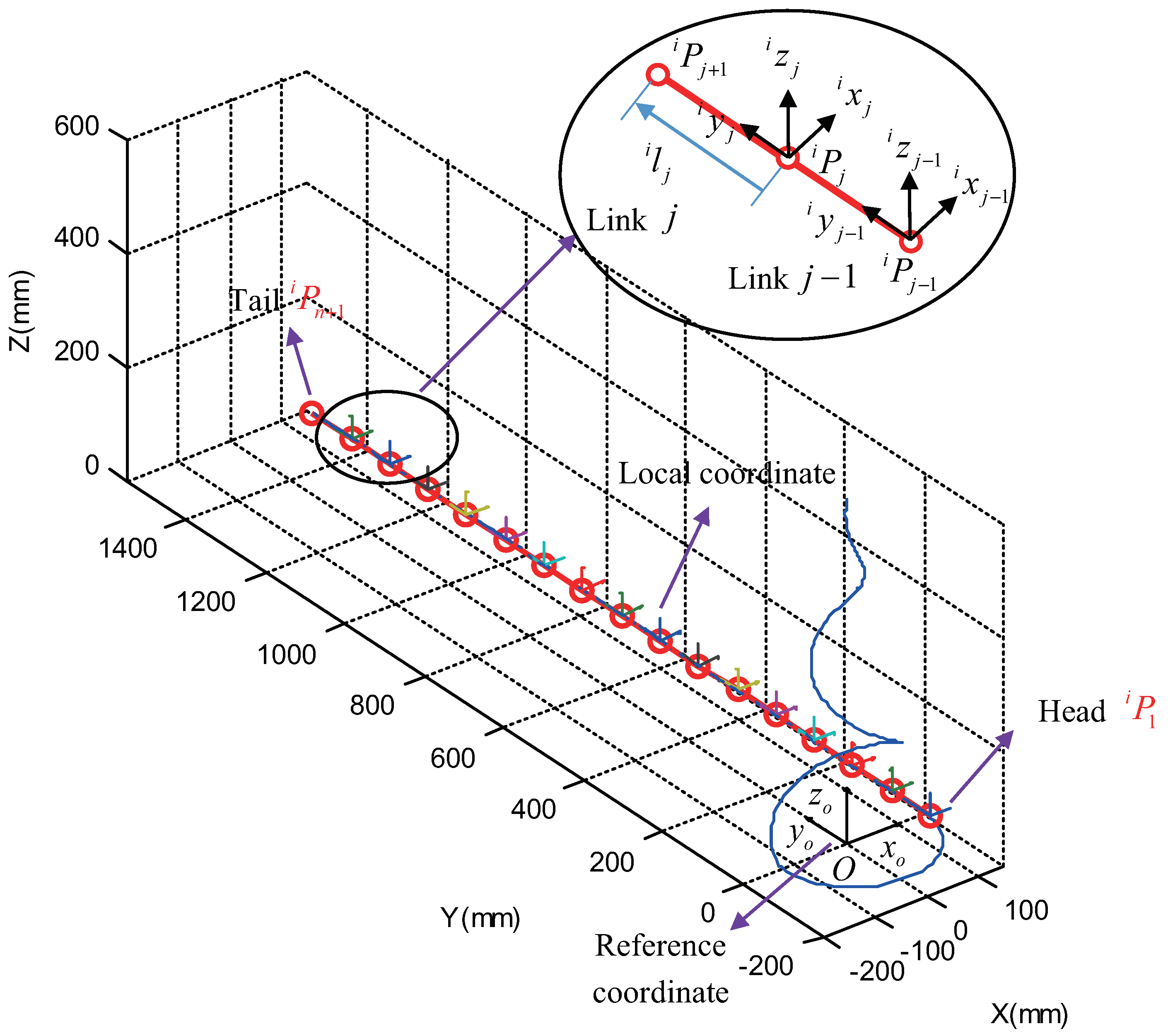
The line segments cannot contain all the information of the snake robot links or modules. Therefore, we propose an approach on establishing the coordinate system fixed on line segments.

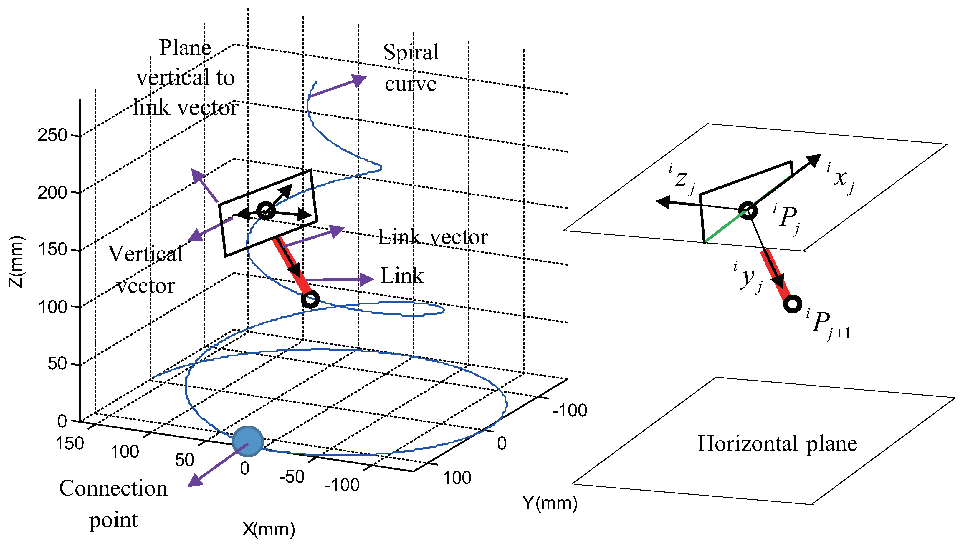
Figure 5 shows the reference coordinate $O_{x_o{y}_o{z}_o}$, and its origin is $[0,0,0]$, with $x_o$-axis $[1,0,0]$, $y_o$-axis $[0,1,0]$, and $z_o$-axis $[0,0,1]$. In determining the local coordinates, several rules are needed. Figure 6 shows how these rules are established and illustrates one link at step i during the phase-shifting process. The ${}^i{y}_j$-axis is calculated as follows:

$${}^i{y}_j=\frac{{}^i{p}_{j+1}-{}^i{p}_j}{∥{}^i{p}_{j+1}-{}^i{p}_j∥}$$

(10)

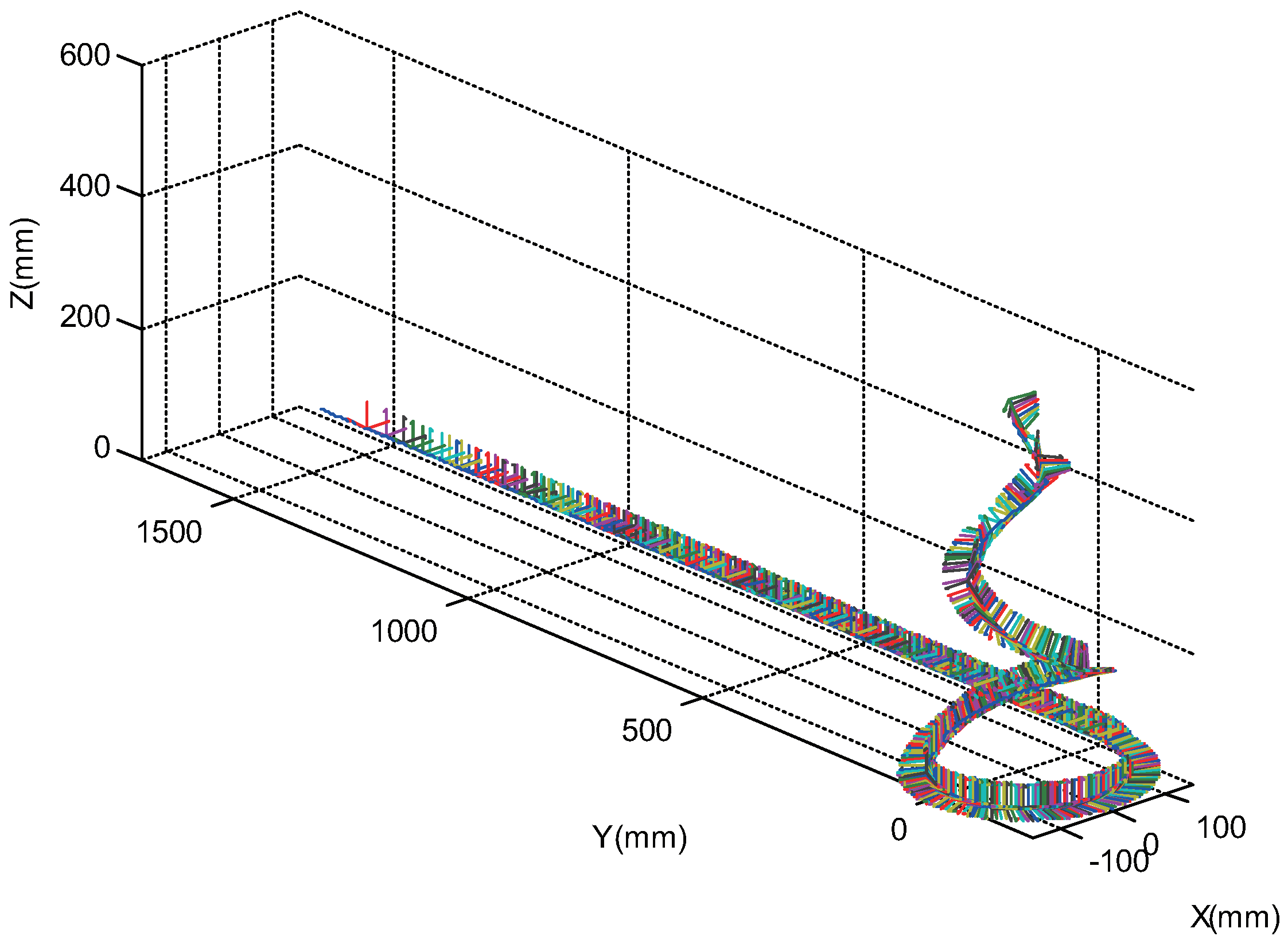
The ${}^i{x}_j$- and ${}^i{z}_j$-axes are on the plane that is vertical to the link vector shown in the left part of Figure 6. Therefore, the ${}^i{x}_j$- and ${}^i{z}_j$-axes are not unique, and the horizontal plane is introduced to solve this problem. Moving the horizontal plane to point ${}^i{P}_j$, the intersecting line between two planes is used to select the ${}^i{x}_j$-axis, as shown in the right part of Figure 6. The intersecting line has two directions. Thus, the direction is selected by determining whether the angle between ${}^i{x}_j$- and $x_o$-axes is acute. Afterward, the ${}^i{z}_j$-axis is determined using the right-hand rule. Figure 7 shows the result of the local coordinates during the entire phase-shifting process. The simulation without showing the coordinates is discussed in the subsequent chapter.

After the determination of the coordinate system, the relative rotation matrix between adjacent links can be obtained using Equation (11).

$$\begin{array}{c}{}^i{R}_{P\_re{l}_j}={({}^i{R}_{P_{j+1}})}^{-1}{(}^i{R}_{P_j})j=2,3\dots ,ni=1,2,\dots ,n_{step}\hfill \\ {}^i{R}_{P_j}=\left[\begin{array}{ccc}{}^i{x}_j& {}^i{y}_j& {}^i{z}_j\end{array}\right]=\left[\begin{array}{ccc}{r}_{11}& r_{12}& r_{13}\\ r_{21}& r_{22}& r_{23}\\ r_{31}& r_{32}& r_{33}\end{array}\right]\hfill \end{array}$$

(11)

where ${}^i{R}_{P_j}\in R^{3\times 3}$ is the orientation matrix of link j relative to the reference coordinate and ${}^i{R}_{P\_re{l}_j}\in R^{3\times 3}$ is the orientation matrix of link j relative to ${}^i{R}_{P_{j+1}}$. Then, the relative roll (${}^i{\gamma }_j$), pitch (${}^i{\beta }_j$), and yaw (${}^i{\alpha }_j$) angle sequences can be calculated using Equation (12).

$$\begin{array}{c}{}^i{\beta }_j=Atan2(-r_{31},\sqrt{{r_{11}}^2+{r_{21}}^2})j=2,3\dots ,ni=1,2,\dots ,n_{step}\hfill \\ {}^i{\alpha }_j=Atan2(r_{21}/cos({}^i{\beta }_j),r_{11}/cos({}^i{\beta }_j))\hfill \\ {}^i{\gamma }_j=Atan2(r_{32}/cos({}^i{\beta }_j),r_{33}/cos({}^i{\beta }_j))\hfill \end{array}$$

(12)

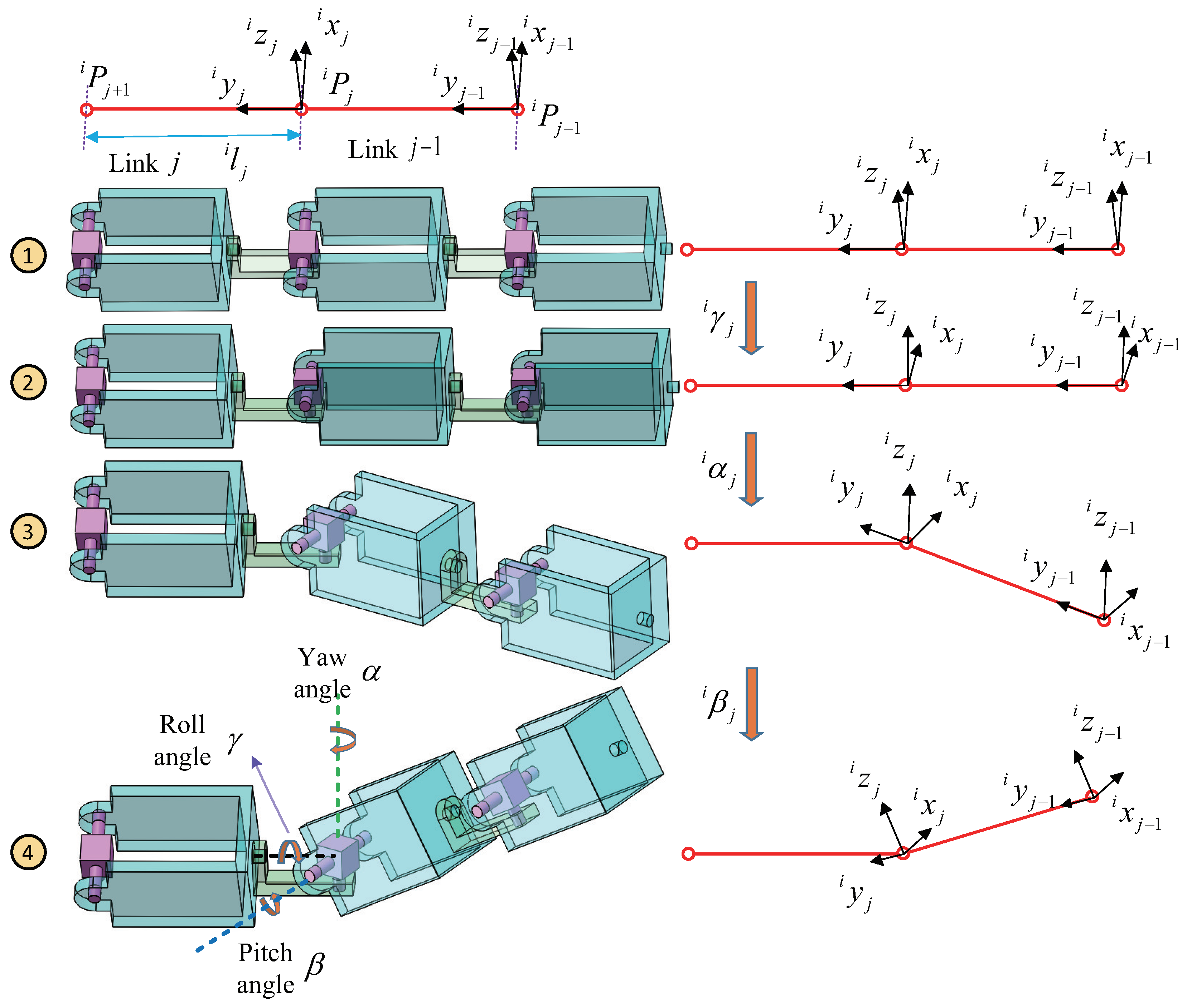
The line segments model for the snake robot is abstract, therefore we introduce a simplified Solidworks model for the subsequent simulation in Adams environment, as shown in Figure 8. It is part of Solidworks model and contains three modules. This figure provides us with the line segments model (right part) and Solidworks model (left part), and it is convenient for us to understanding where local coordinates are established and how the roll, pitch, and yaw angles are solved. As mentioned before, a line segment (${}^i{l}_j$) and a local coordinate (${}^i{P}_j-{}^i{x}_j{}^i{y}_j{}^i{z}_j$) represent a snake robot module, and a point (${}^i{P}_j$) represents a joint with three degrees of freedom. The three axes are located at centers of rotating shafts and intersected at the ${}^i{P}_j$. Connecting the ${}^i{P}_j$ and the ${}^i{P}_{j+1}$, the ${}^i{l}_j$ can be determined. Equation (11) and (12) provide us with the solution of roll, pitch and yaw angles. However, it is significant to determine their rotating sequences, which are also illustrated in Figure 8. It should be pointed out that the rotating sequences depend on specific models, otherwise, the rotating sequences and Equation (12) should be modified.

3. Simulation on Head-Raising Motion

According to the proposed algorithms, the phase-shifting process can be simulated. The parameters of the predefined curve are as follows: $a=9.7$, $b=1$, $c=48.5$, $n_c=2.5$, $n=16$, $l_{link}=97$ (mm), ${\widehat{t}}_1=1,552$ (rad), ${\widehat{t}}_2=1,555.1$ (rad), ${\widehat{t}}_3=1,567.7$ (rad), ${\phi }_0=1.6022$ (rad), and ${\phi }_{base}=pi$ (rad). According to Equation (3), the arc lengths of BS ($S_1$) and RS ($S_2$) can be calculated as $S_1=431.8891$ (mm) and $S_2=1,032.6$ (mm). The discrete independent variable is selected as $t_d=[0,0.1,0.2,\dots ,{\widehat{t}}_1,{\widehat{t}}_1+0.001,{\widehat{t}}_1+0.002,\dots ,{\widehat{t}}_3]$ with $\Delta t_1=0.1$ and $\Delta t_2=0.001$. To facilitate reading, all the symbols utilized in this paper are concluded in Appendix part, as shown in

Table A1. Symbols utilized in this paper.

Symbol	Definition
$x_l(t)$	x value of line part in the predefined spiral curve
$y_l(t)$	y value of line part in the predefined spiral curve
$z_l(t)$	z value of line part in the predefined spiral curve
$x_s(t)$	x value of spiral curve part in the predefined spiral curve
$y_s(t)$	y value of spiral curve part in the predefined spiral curve
$z_s(t)$	z value of spiral curve part in the predefined spiral curve
a	Adjustment coefficient of the spiral curve, which can be used to change the amplitude of $x_s(t)$ and $y_s(t)$ equally
b	Adjustment coefficient of the spiral curve, which can be used to change the amplitude of $x_s(t)$ and $y_s(t)$ unequally
c	Adjustment coefficient of the spiral curve, which can be used to change the amplitude of $z_s(t)$
${\phi }_0$	Initial phase of the sine and cosine functions
$n_c$	Cycle number of the spiral curve
$l_{link}$	Length of the snake robot modules
n	Number of the snake robot modules
t	Independent variable divided into three intervals: $(0,{\widehat{t}}_1)$, $({\widehat{t}}_1,{\widehat{t}}_2)$ and $({\widehat{t}}_2,{\widehat{t}}_3)$
$y_s(t)$	y value of spiral curve part in the predefined spiral curve
LP	Line part of the predefined spiral curve, corresponding to interval $(0,{\widehat{t}}_1)$
BS	The base of the spiral curve part, which is in contact with the ground and corresponds to interval $({\widehat{t}}_1,{\widehat{t}}_2)$
RS	y The base of the spiral curve part, which is in contact with the ground and corresponds to interval $({\widehat{t}}_2,{\widehat{t}}_3)$
${\widehat{t}}_1$	Value of t connecting LP and BS
${\widehat{t}}_2$	Value of t connecting BS and RS
${\widehat{t}}_3$	End value of t
${\phi }_{base}$	The phase value of interval $({\widehat{t}}_1,{\widehat{t}}_2)$
$t_i$	y Discrete value of simulation time
i	Index value of simulation step
j	Index value of point P in line segments model of the snake robot
${}^i{P}_j$	Position of point j step i of phase-shifting process
$n_{step}$	Number of phases shifted
${}^i{x}_{snk\_j}$	x value of ${}^i{P}_j$
${}^i{y}_{snk\_j}$	y value of ${}^i{P}_j$
${}^i{z}_{snk\_j}$	z value of ${}^i{P}_j$
$\Delta S_i$	Arc length at step i and defined as “phase”
${}^i{P}_{snk}$	Point set at step i
$t_d$	y Discrete vector of t
$\Delta t_1$	Step length of discretization in interval $(0,{\widehat{t}}_1)$
$\Delta t_2$	Step length of discretization in interval $({\widehat{t}}_1,{\widehat{t}}_3)$
${}^{i}In{x}_{pj}$	Index value of element in $t_d$, which is nearest to $t_{i+1}$ during phase-shifting process
$eps$	Threshold utilized to deal with the error between continuous function and discrete approximation
$O_{x_o{y}_o{z}_o}$	Reference coordinate
${}^i{x}_j$	x coordinate axis fixed on the snake module j at step i
${}^i{y}_j$	y coordinate axis fixed on the snake module j at step i
${}^i{z}_j$	z coordinate axis fixed on the snake module j at step i
${}^i{l}_j$	Link vector connecting ${}^i{P}_j$ and ${}^i{P}_{j+1}$
${}^i{P}_j-{}^i{x}_j{}^i{y}_j{}^i{z}_j$	y Local coordinate fixed on link $j-1$
${}^i{\alpha }_j$	Yaw angle of joint j at step i
${}^i{\beta }_j$	Pitch angle of joint j at step i
${}^i{\gamma }_j$	Roll angle of joint j at step i
${}^i{\dot{\alpha }}_j$	Yaw angular velocity of joint j at step i
${}^i{\dot{\beta }}_j$	Pitch angular velocity of joint j at step i
${}^i{\dot{\gamma }}_j$	Roll angular velocity of joint j at step i
${}^i{\ddot{\alpha }}_j$	Yaw angular acceleration of joint j at step i
${}^i{\ddot{\beta }}_j$	Pitch angular acceleration of joint j at step i
${}^i{\ddot{\gamma }}_j$	Roll angular acceleration of joint j at step i
$t_{time}$	Head-raising motion time
${}^i{R}_{P_j}$	Orientation matrix of link j with respect to the reference coordinate at step i
${}^i{R}_{P\_re{l}_j}$	Orientation matrix of link j with respect to ${}^i{R}_{P_{j+1}}$ at step i
$R_x(.)$	Matrix involving vector rotating around the x axis
$R_y(.)$	Matrix involving vector rotating around the y axis
$R_z(.)$	Matrix involving vector rotating around the z axis

.

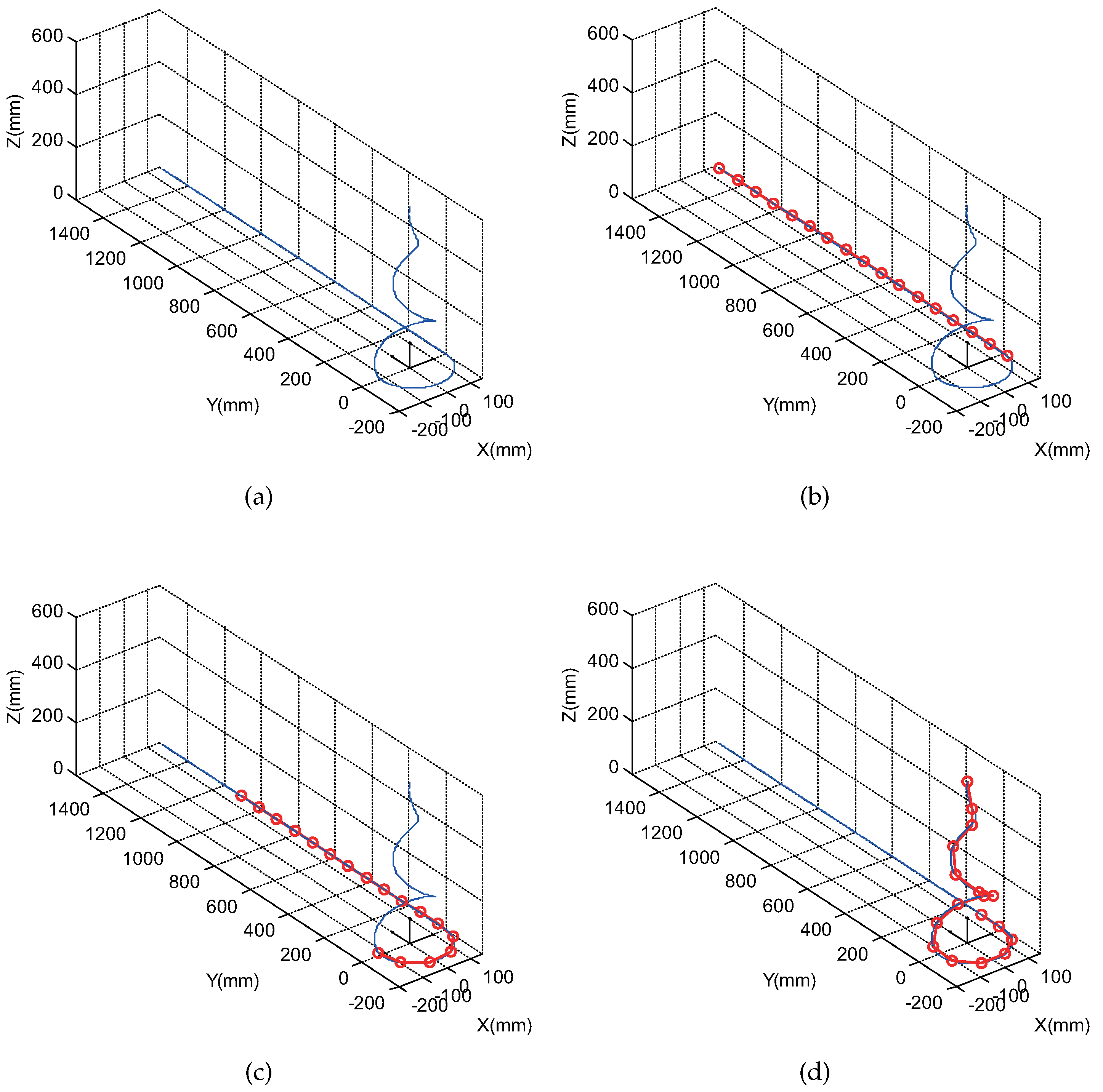
The snake begins to move from basic posture to final posture using the shape-fitting and phase-shifting algorithms. During the phase-shifting process, the phase $\Delta S_i$ in every step can be selected manually. In this test, $\Delta S_i$ is assumed constant and equal to $(S_1+S_2)/n_{step}$, where the number of total steps $n_{step}$ equals 500.

Table 1. Data during phase-shifting process.

Step i	Head ${}^{\mathit{i}}{\mathit{P}}_1$ (mm)	Index of Head ${}^{\mathit{i}}\mathit{In}{\mathit{x}}_{{\mathit{p}}_1}$	Yaw Angle ${}^{\mathit{i}}{\mathit{\alpha }}_1$ (rad)	Pitch Angle ${}^{\mathit{i}}{\mathit{\beta }}_1$ (rad)	Roll Angle ${}^{\mathit{i}}{\mathit{\gamma }}_1$ (rad)
1	(151.8, −12.8, 0)	15,520	0	0	0
2	(151.3, −15.7, 0)	15,541	−0.0047	0	0
⋮	⋮	⋮	⋮	⋮	⋮
300	(57.3, −61.8, 188.1)	22,544	−0.8964	0.2259	−0.3775
⋮	⋮	⋮	⋮	⋮	⋮
499	(−0.546, 0.015, 606.7)	31,174	−2.5001	2.1308	−0.8348
500	(−0.0036, −0.003, 609.4)	31,230	−2.5309	2.1658	−0.8225

shows the data of ${}^i{P}_1$, ${}^{i}In{x}_{p_1}$, ${}^i{\alpha }_1$, ${}^i{\beta }_1$, and ${}^i{\gamma }_1$ at steps 1, 2, 300, 499, and 500, respectively. Figure 9 shows the phase-shifting process, including the predefined spiral curve (Figure 9a) and snake posture at steps $i=1$ (Figure 9b), $i=147$ (Figure 9c), and $i=500$ (Figure 9d), corresponding to the snake head at $t={\widehat{t}}_1$, $t={\widehat{t}}_2$, and $t={\widehat{t}}_3$, respectively.

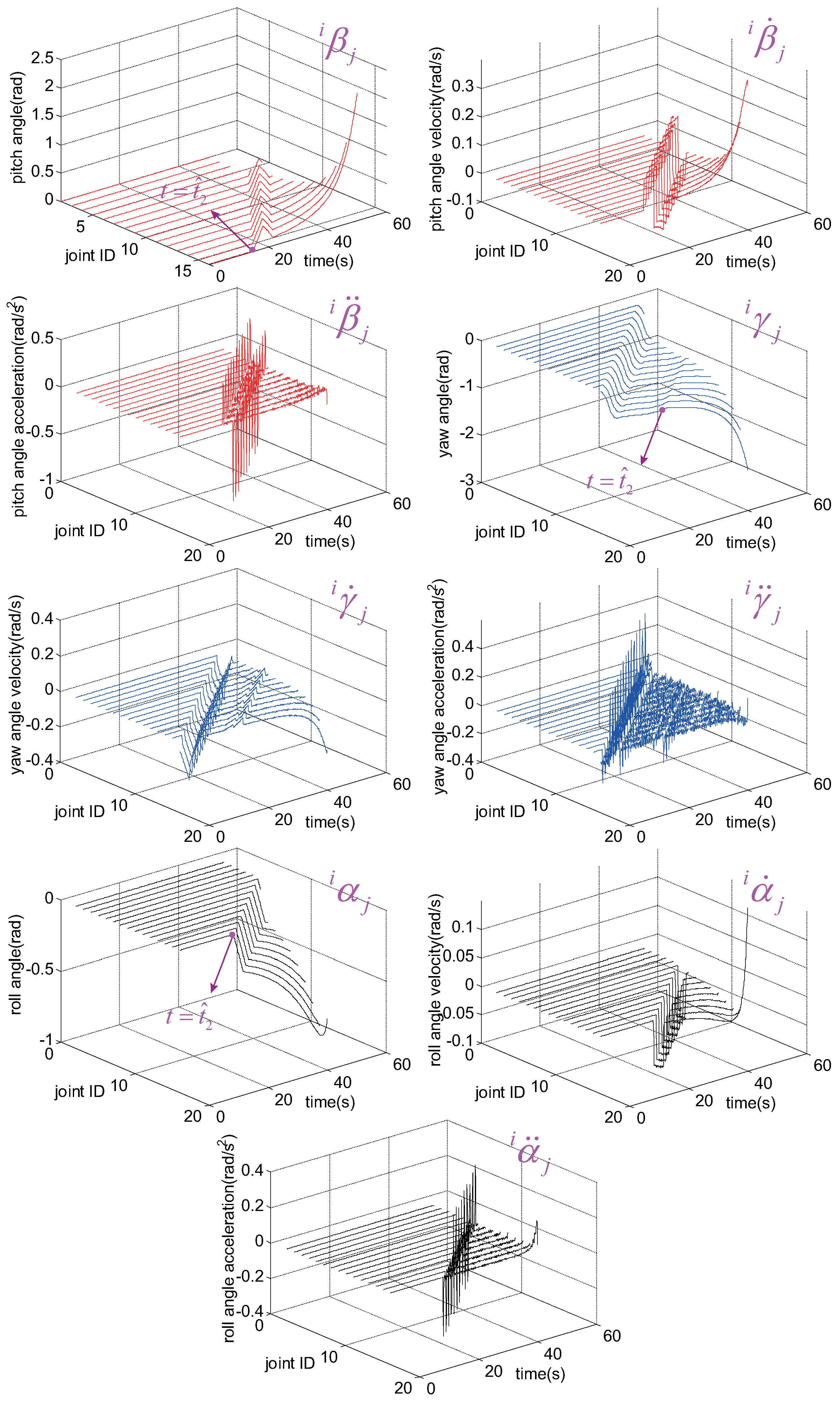
We assume that the head-raising motion time is 50 s, that is, $t_{time}\in (0,50)$. With Equation (12) and numerical derivation, the roll (${}^i{\gamma }_j$), pitch (${}^i{\beta }_j$), and yaw (${}^i{\alpha }_j$) angle sequences; relative angular velocity (${}^i{\dot{\gamma }}_j,{}^i{\dot{\beta }}_j,{}^i{\dot{\alpha }}_j$); and angular acceleration (${}^i{\ddot{\gamma }}_j,{}^i{\ddot{\beta }}_j,{}^i{\ddot{\alpha }}_j$) can be obtained, as shown in the z-axis of Figure 10. The x- and y-axes represent the joint ID ($ID=1,2,\dots ,15$) and time, respectively. As the snake head moves from $t={\widehat{t}}_1$ to $t={\widehat{t}}_2$, the absolute value of ${}^i{\gamma }_1$ initially increases before the third joint point moves to $t={\widehat{t}}_1$ and subsequently becomes constant because the first two links are constrained to a semicircle. Meanwhile, the absolute values of ${}^i{\alpha }_1$ and ${}^i{\beta }_1$ are zero. Similarly, the motion of the snake head moving from $t={\widehat{t}}_2$ to $t={\widehat{t}}_3$ can be divided into two stages. Before the third joint point moves to $t={\widehat{t}}_2$, the absolute value of ${}^i{\gamma }_1$ initially decreases in the first stage and then subsequently increases in the second stage. In the meantime, the absolute value of ${}^i{\alpha }_1$ increases at varying speed. The absolute value of ${}^i{\beta }_1$ initially increases, subsequently decreases, and finally increases. Unsmooth angles are caused by the unsmooth transition of the piecewise function, which will be improved in future work. Thus, the shapes of the relative velocity and acceleration curve are full of sharp points. Moreover, the curves of the other joint points ($ID=2,3,\dots ,15$) have the same shape with phase lag.

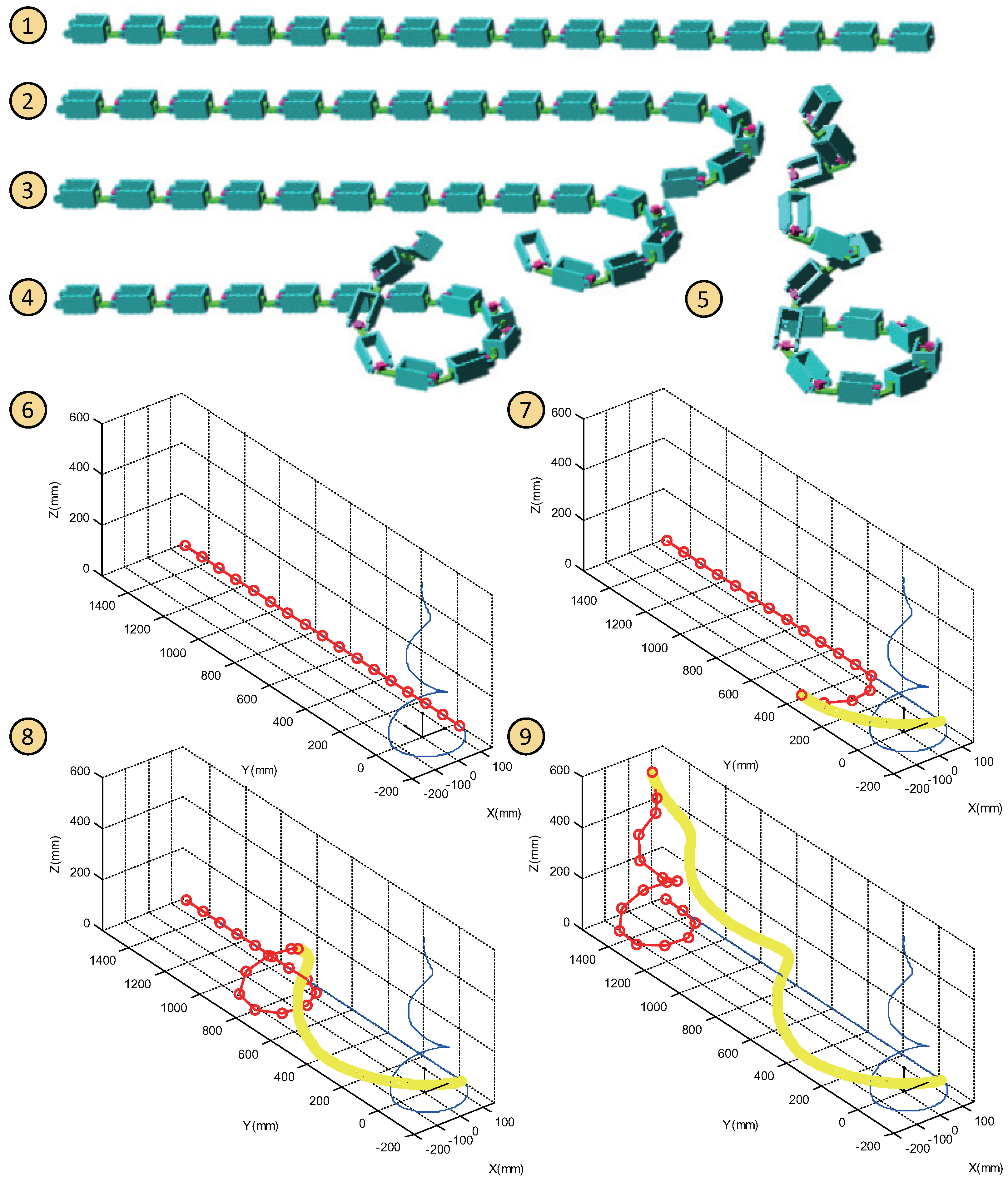
Distinguishing between the phase-shifting and head-raising processes is important. The phase-shifting process is used to obtain the joint trajectory and does not exist in reality if the snake robot has no active wheels with which to move its body along the predefined spiral curve. Meanwhile, the head-raising process is the actual head-raising motion produced using the joint trajectory, and in this case, the tail of the snake robot is fixed. Figure 11 shows the two kinds of simulations of head-raising process. Those simulations are in kinematic level and do not take dynamic factors into consideration. The Simulation in labels 1–5 are implemented in Adams, and the roll, pitch and roll angles are integrated into spline curves to guide the model’s movement. The simulation in labels 6–9 are carried out using Matlab, based on the following algorithm:

(1)

Determine the basic posture as Equation (6), and set motion step $i=1$;

(2)

Proceed to motion step $i=2$. The link n is fixed. Calculate the position of link $n-1$ on the basis of angles ${}^2{\alpha }_n$, ${}^2{\beta }_n$, and ${}^2{\gamma }_n$;

(3)

Make an iteration to calculate all of the positions of the links, that is, link $j=n-2,n-3,\dots ,1$, on the basis of angles $({}^2{\alpha }_{n-2},{}^2{\beta }_{n-2},{}^2{\gamma }_{n-2})$, $({}^2{\alpha }_{n-3},{}^2{\beta }_{n-3},{}^2{\gamma }_{n-3}),\dots ,({}^2{\alpha }_1,{}^2{\beta }_1,{}^2{\gamma }_1)$;

(4)

Proceed to motion step $i=i+1$ and repeat steps 2 and 3 until $i=n_{step}$.

In this algorithm, step 2 is important. During the phase-shifting and head-raising processes, their link vectors ${}^i{l}_j$, as shown in Figure 5, are same in orientation and different in position. Therefore, the position of joint point ${}^i{P}_j$ can be obtained as follows:

$$\begin{array}{c}{}^i{l}_{j-1}={}^i{l}_j{R}_z({}^i{\alpha }_j)R_y({}^i{\alpha }_j)R_x({}^i{\alpha }_j)\hfill \\ {}^i{P}_j={}^i{P}_{j-1}+{}^i{l}_{j-1}\hfill \\ R_z({}^i{\alpha }_j)=\left[\begin{array}{ccc}cos({}^i{\alpha }_j)& -sin({}^i{\alpha }_j)& 0\\ sin({}^i{\alpha }_j)& cos({}^i{\alpha }_j)& 0\\ 0& 0& 1\end{array}\right]R_y({}^i{\beta }_j)=\left[\begin{array}{ccc}cos({}^i{\beta }_j)& 0& sin({}^i{\beta }_j)\\ 0& 1& 0\\ -sin({}^i{\beta }_j)& 0& cos({}^i{\beta }_j)\end{array}\right]\hfill \\ R_z({}^i{\gamma }_j)=\left[\begin{array}{ccc}1& 0& 0\\ 0& cos({}^i{\gamma }_j)& -sin({}^i{\gamma }_j)\\ 0& sin({}^i{\gamma }_j)& cos({}^i{\gamma }_j)\end{array}\right]\hfill \end{array}$$

(13)

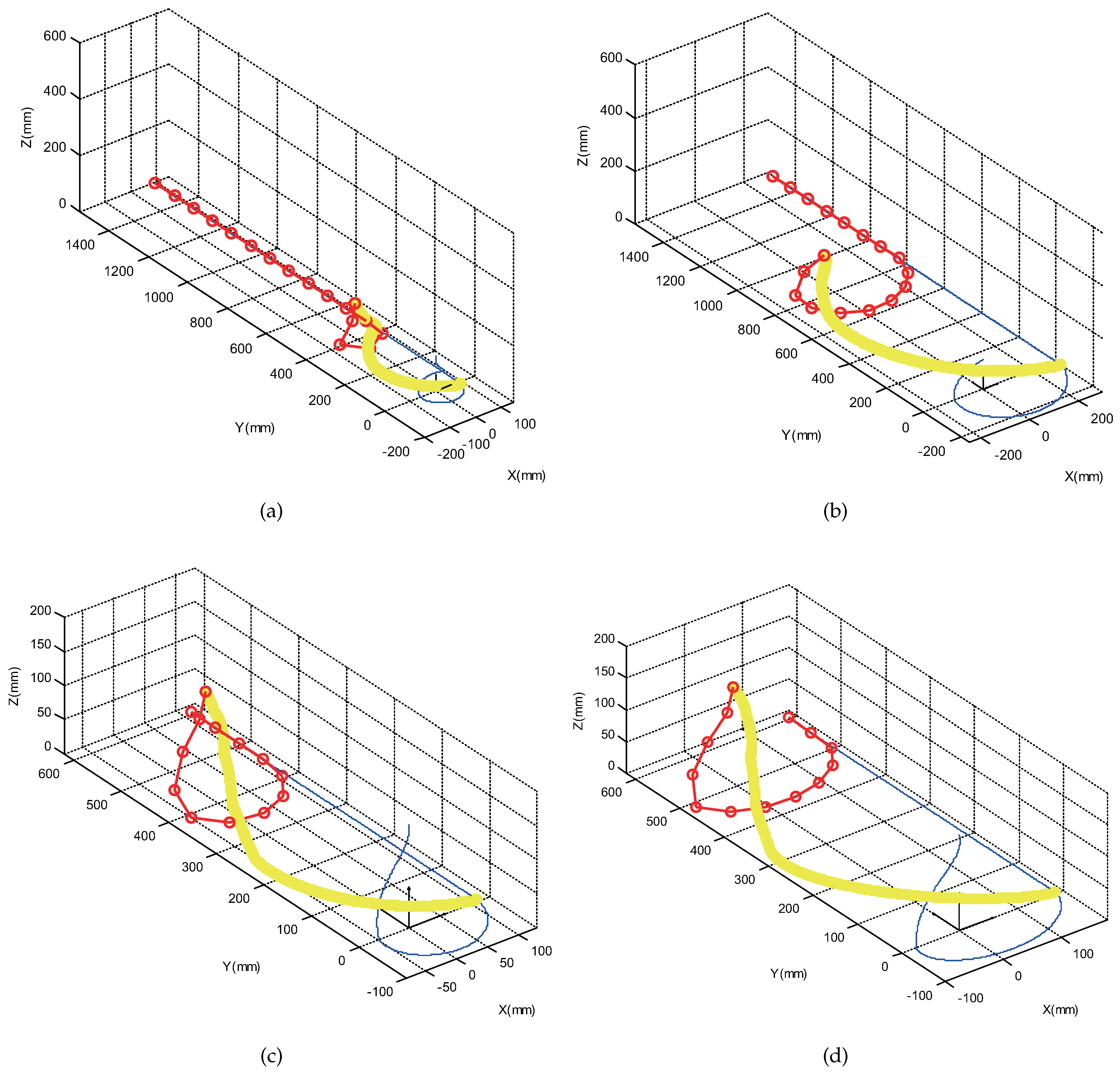
Considering that the method of head-raising should be adaptive to deal with different situations, more simulations are implemented as described in Figure 12, where different parameters of the predefined spiral curves are adopted and they are listed in

Table 2. Parameters of predefined spiral curves used in head-raising simulations shown in Figure 11 and Figure 12.

Figure Number	a	b	c	${\mathit{n}}_{\mathit{c}}$	${\mathit{\phi }}_0$ (rad)	n	${\mathit{l}}_{\mathit{link}}$ (mm)
Figure 11	9.7	1	48.5	2.5	0.5 pi	16	97
Figure 12a	9.7	1	20	1.5	0.5 pi	16	97
Figure 12b	60	1	60	0.8	0.5 pi	16	97
Figure 12c	20	1	60	0.9	1.5 pi	12	50
Figure 12d	20	1.5	60	0.9	1.5 pi	12	50

. In Figure 12, only final postures are shown, and more detailed simulations can be found in Supplementary Materials. Compared with the result in Figure 11 and Figure 12a, the radius of the supporting part BS becomes larger when increasing the value of parameter a (Figure 12b–d); the height of every circle becomes larger if the parameter c increases (Figure 12b–d). When changing the parameter b, the amplitudes of $x_s(t)$ and $y_s(t)$ change unequally. Additionally, the LP part changes accordingly (Figure 12c,d) when changing the parameters $l_{link}$ and n, and it should be noted that ${\phi }_0$ is set to ensure the initial phases of the sine and cosine functions. All the simulations confirm the feasibility and validity of the proposed method.

4. Discussion and Conclusions

In this study, head-raising motion of a snake robot based on a predefined spiral curve is proposed and relative simulations are conducted. Obtaining the angle sequences of the head-raising motion of snake robots is difficult under three-dimensional conditions. Thus, the proposed method adopts the predefined spiral curve to guide the robot in moving, thereby improving the performance of the robot and laying the foundation for accomplishing additional tasks. The predefined spiral curve is parameterized. With changes in the parameters, the curves can adapt to different lengths and numbers of the snake robot modules, spiral numbers, and heights of head-raising.

However, there are some problems to be solved in the future work. First, the predefined spiral curve is a piecewise function and has unsmooth points, thus leading to sharp changes in motion trajectories. Second, our model considers only kinematic planning, that is, the dynamic problem is not considered. Dynamic constraints are important factors for successful implementation of our model on a real robot, and will be added into an improved model in the future work. At the same time, experimental verification will be carried out in the next phase of research, after finishing the design and construction of the platform. The greatest challenge to use our model on a real robot is that the robot has to overcome the gravity during the head-raising, and the actuation system must be equipped with motors which have adequate torques to drive the snake modules. The work in [13] is a successful example although they adopted a different method to raise the robot’s head. When designing the prototype, lightweight materials can be used to enable the robot with lighter gravity and stronger driving power. More importantly, our model is adaptive. As illustrated in Figure 12, by decreasing the height, the cycle number and increasing the radius of supporting part, it is feasible for the robot to raise its head while satisfying the dynamic constraints. In some specific situations such as exploring the moon, and searching for resources underwater, the gravity will decrease or be compensated. Then, it will be easier for the robot to raise their head. Third, the head-raising motion forms of snake in the natural world can change over time. To accomplish that, the predefined spiral curve should be made time varying without influencing the stability of the robot body, and this principle will also be the focus of the future research.

References

- Transeth, A.A.; Pettersen, K.Y.; Liljebäck, P. A survey on snake robot modeling and locomotion. Robotica 2009, 27, 999–1015. [Google Scholar] [CrossRef]
- Liljebäck, P.; Pettersen, K.Y.; Stavdahl, Ø.; Gravdahl, J.T. A review on modelling, implementation, and control of snake robots. Robot. Auton. Syst. 2012, 60, 29–40. [Google Scholar] [Green Version]
- Liu, J.; Wang, Y.; Li, B.; Ma, S. Path planning of a snake-like robot based on serpenoid curve and genetic algorithms. In Proceedings of the 5th World Congress on Intelligent Control and Automation, Hangzhou, China, 15–19 June 2004; pp. 4860–4864. [Google Scholar]
- Saito, M.; Fukaya, M.; Iwasaki, T. Serpentine locomotion with robotic snakes. IEEE Control Syst. Mag. 2002, 22, 64–81. [Google Scholar] [CrossRef]
- Chen, L.; Wang, Y.; Ma, S.; Li, B. Analysis of traveling wave locomotion of snake robot. In Proceedings of the 2003 IEEE International Conference on Robotics, Intelligent Systems and Signal Processing, Changsha, China, 8–13 October 2003; pp. 365–369. [Google Scholar]
- Kalani, H.; Akbarzadeh, A.; Safehian, J. Traveling wave locomotion of snake robot along symmetrical and unsymmetrical body shapes. In Proceedings of the 41st International Symposium on Robotics and 6th German Conference on Robotics, Munich, Germany, 7–9 June 2010; pp. 62–68. [Google Scholar]
- Liu, J.; Wang, Y.; Li, B.; Chen, L.; Ma, S. Serpentine locomotion with robotic snakes. Chin. J. Mech. Eng. 2005, 41, 108–113. [Google Scholar] [CrossRef]
- Virgala, I.; Dovica, M.; Kelemen, M.; Prada, E.; Bobovsky. Snake robot movement in the pipe using concertina locomotion. Jixie Gongcheng Xuebao/Chin. J. Mech. Eng. 2005, 41, 108–113. [Google Scholar] [CrossRef]
- Chen, L.; Wang, Y.; Ma, S.; Li, B. Study of lateral locomotion of snake robot. Robot 2003, 25, 246–249. [Google Scholar]
- Tanev, I.; Ray, T.; Buller, A. Evolution, robustness, and adaptation of sidewinding locomotion of simulated snake-like robot. In Genetic and Evolutionary Computation Conference; Springer: Berlin, Germany, 2004; pp. 627–639. [Google Scholar]
- Wang, K.; Gao, W.; Ma, S. Snake-like robot with fusion gait for high environmental adaptability: Design, modeling, and experiment. Appl. Sci. 2017, 7, 1133. [Google Scholar] [CrossRef]
- Sanfilippo, F.; Azpiazu, J.; Marafioti, G.; Transeth, A.A.; Stavdahl, Ø.; Liljebäck, P. Study of lateral locomotion of snake robot. Appl. Sci. 2017, 7, 336. [Google Scholar] [CrossRef]
- Ye, C.; Ma, S.; Li, B.; Wang, Y. Head-raising motion of snake-like robots. In Proceedings of the 2004 IEEE International Conference on Robotics and Biomimetics, Shenyang, China, 22–26 August 2004; pp. 595–600. [Google Scholar]
- Tanaka, M.; Matsuno, F. Modeling and control of head raising snake robots by using kinematic redundancy. J. Intell. Robot. Syst. 2014, 75, 53–69. [Google Scholar] [CrossRef]
- Cappo, E.A.; Choset, H. Planning end effector trajectories for a serially linked, floating-base robot with changing support polygon. In Proceedings of the 2004 American Control Conference, Portland, OR, USA, 4–6 June 2014; pp. 4038–4043. [Google Scholar]
- Wu, W.; Hong, Y.; Wang, G. Geometrical spline approach to shape control of super redundant planar manipulator. Mach. Tool Hydraul. 2004, 4, 70–72. [Google Scholar]
- Nor, N.M.; Ma, S. Body shape control of a snake-like robot based on phase oscillator network. In Proceedings of the 2013 IEEE International Conference on Robotics and Biomimetics, Shenzhen, China, 12–14 December 2013; pp. 274–279. [Google Scholar]
- Liljebäck, P.; Pettersen, K.Y.; Stavdahl, O.; Gravdahl, J.T. A control framework for snake robot locomotion based on shape control points interconnected by Bézier curves. In Proceedings of the 2012 IEEE/RSJ International Conference on Intelligent Robots and Systems, Algarve, Portugal, 7–12 October 2012; pp. 3111–3118. [Google Scholar]
- Tanaka, M.; Tanaka, K. Shape Control of a snake robot with joint limit and self-collision avoidance. IEEE Trans. Control Syst. Technol. 2017, 25, 1441–1448. [Google Scholar] [CrossRef]
- Liu, J.; Wang, Y.; Ma, S.; Li, B. Shape control of hyper-redundant modularized manipulator using variable structure regular polygon. In Proceedings of the 2004 IEEE/RSJ International Conference on Intelligent Robots and Systems, Sendai, Japan, 28 September–2 October 2004; pp. 3924–3929. [Google Scholar]
- Chirikjian, G.S.; Burdick, J.W. A modal approach to hyper-redundant manipulator kinematics. IEEE Trans. Robot. Autom. 1994, 10, 343–354. [Google Scholar] [CrossRef] [Green Version]
- Burdick, J.W.; Radford, J.; Chirikjian, G.S. A “sidewinding” locomotion gait for hyper-redundant robots. Adv. Robot. 1995, 9, 195–216. [Google Scholar] [CrossRef]
- Hatton, R.L.; Choset, H. Generating gaits for snake robots by annealed chain fitting and keyframe wave extraction. Auton. Robot. 2010, 28, 271–281. [Google Scholar] [CrossRef]
- Tavakkoli, S.; Dhande, S.G. Shape synthesis and optimization using intrinsic geometry. J. Mech. Des. 1991, 113, 379–386. [Google Scholar] [CrossRef]
- Mochiyama, H.; Shimemura, E.; Kobayashi, H. Shape control of manipulators with hyper degrees of freedom. Int. J. Robot. Res. 1999, 18, 584–600. [Google Scholar] [CrossRef]
Figure 1.
The concepts of 2D and 3D head-raising. Label 1 and 2 represent 2D head-raising, and label 3 and 4 show 3D head-raising.
Figure 2.
The similar macro shapes of a snake (label 1), a spiral curve (label 2), the line segments model after the shape-fitting algorithm (label 3) and the simplified simulation model (label 4).
Figure 3.
Spiral curves: (a) the regular spiral curve, and (b) the predefined spiral curve used in this study.
Figure 4.
Concepts of shape-fitting and phase-shifting.
Figure 5.
Modeling of the robot’s basic posture composed of n line segments and corresponding coordinate system.
Figure 6.
Establishment of local coordinates.
Figure 7.
Local coordinates during entire head-raising process.
Figure 8.
Local coordinates fixed on the simplified Solidworks model and descriptions of roll, pitch and yaw angles. Label 1 corresponds to the initial configuration. Label 2, 3 and 4 describe the configurations after rotating roll angle, yaw angle and pitch angle, respectively.
Figure 9.
Phase-shifting process: (a) predefined spiral curve, (b) , , (c) , , (d) , .
Figure 10.
Angle, angular velocity, and angular acceleration during phase-shifting process.
Figure 11.
Head-raising motion process. Labels 1–5 show different states from initial posture to final posture of head-raising in Adams environment. Label 1 is the initial posture and label 5 is the final posture. Label 2 corresponds to the case that the robot forms a supporting configuration. Label 3 and 4 are intermediate states. The labels 6–9 are head-raising simulations of line segments model, implemented in Matlab environment. The labels 6–9 correspond to labels 1, 2, 4 and 5, respectively.
Figure 12.
Head-raising motion process with different parameters of the predefined spiral curve, and the parameters are listed in Table 2.