Effects of Anisotropic Turbulence on Propagation Characteristics of Partially Coherent Beams with Spatially Varying Coherence

Abstract

Based on the extended Huygens-Fresnel (eHF) principle, approximate analytical expressions for the spectral density of nonuniformly correlated (NUC) beams are derived with the help of discrete model decompositions. The beams are propagating along horizontal paths through an anisotropic turbulent medium. Based on the derived formula, the influence of the anisotropic turbulence (anisotropy factors, structure parameters) on the evolution of the average intensity, the shift of the intensity maxima and the power-in-the-bucket (PIB) are investigated in detail through numerical examples. It is found that the lateral shifting of the intensity maxima is closely related to the anisotropy factors and the strength of turbulence. Our results also reveal that, in the case of weak turbulence, the beam profile can retain the feature of local intensity sharpness, but this feature degenerates quickly if the strength of the turbulence increases. The value of PIB of the NUC beams can be even higher than that of Gaussian beams by appropriately controlling the coherence parameter in the weak turbulence regime. This feature makes the NUC beams useful for free-space communication.

1. Introduction

The study of laser beams propagation through the atmosphere has received wide attention due to its important applications in high-speed/high-capacity free-space optical communications and remote sensing. In these systems, the laser beams experience random refractive index fluctuations induced by atmospheric turbulence. This turbulence gives rise to extra beam broadening, beam wander and scintillation, which limits the performance of these systems. Therefore, the knowledge of the atmospheric turbulence and its interaction with light beams are of great importance. Over the past decades, the theory of light beams propagation in isotropic turbulence has been well developed [1]. However, many experimental results showed that anisotropic turbulence can exist in a wide range of altitudes from the earth’s surface [2,3,4,5,6,7,8,9,10,11]. As early as 1970, Consortini and co-workers experimentally found the evidence of anisotropic turbulence near the ground [2]. They measured relative beam wander of two or more parallel narrow beams through a 130 m horizontal path about one meter above the ground and found that the variance of the refractive index fluctuations in the vertical and horizontal direction is different. Dalaudier et al. presented the experimental evidence of the ubiquitous presence of very strong temperature gradients in the vertical direction, compared to those in the horizontal direction, within very thin layers/sheets in the atmosphere up to 25 km from the ground [3]. Grechko et al. investigated the spatial structure of temperature and density in the middle atmosphere through the observations of star scintillations and found strong anisotropy of temperature gradient in the horizontal and vertical direction for heights 12–45 km from the ground [4]. The anisotropy of turbulence in the stratosphere was investigated by Robert and co-workers. They found the existence of anisotropic refractive index fluctuations from balloon-borne observations of stellar scintillation [5]. The generation of anisotropic turbulence in the laboratory and the approach for designing phase screens for anisotropic turbulence were reported in [12,13]. Meanwhile, theoretical models for structure functions or power spectrum densities obeying Kolmogorov or non-Kolmogorov statistics were proposed to describe the anisotropic refractive index fluctuations of the turbulence [5,6,14,15].

Recently, there has been a growing interest in research of the behavior of optical fields in the presence of anisotropic turbulence. Based on the Rytov method, theoretical models for the log-amplitude correlation function, the angle of arrival fluctuation as well as the modulation transfer function of a plane wave and a spherical wave passing through the anisotropic Kolmogorov or non-Kolmogorov atmosphere, have been established [16,17,18,19,20,21,22]. Furthermore, the statistical properties, such as long-term beam spread, scintillation index and beam wander of a Gaussian beam in weak and moderate-to-strong anisotropic turbulence, were investigated by Toselli et al. [23,24,25] and Andrew et al. [26], respectively. On the other hand, another technique, known as the extended Huygens-Fresnel (eHF) principle, has also been applied to study the behavior of laser beams in anisotropic turbulence [27,28,29,30]. The advantage of the eHF method is that it can be used to treat the propagation characteristics for a wide range of optical fields, including partially coherent fields (see [31,32] and reference therein). The validity of this method extends from weak to strong turbulence. However, in these studies using the eHF method, it is assumed that the statistics of the turbulence in the transverse plane orthogonal to the beam propagation axis is isotropic. Thus, the turbulent anisotropy acts only as the modifier to the strength of turbulence. When a light beam propagates along a horizontal path near the ground, the turbulence affects the beam differently in two transverse directions, perpendicular to propagation axis. Recently, we developed a theoretical model for treating the propagation of light beams under this situation, based on the eHF method [33]. The average intensity and coherence properties of the Gaussian-Schell-model beam under such anisotropic turbulence circumstances are investigated in detail and some results are demonstrated in the experiment [34].

Partially coherent beams with spatially varying coherence, named nonuniformly correlated (NUC) beams, were first introduced by Lajunen and Saastamoinen [35]. Different from Schell-model sources, whose coherence distributions are uniform over the whole field, The NUC beams have a locally varying degree of coherence. Owing to its unique coherence properties, the NUC beams exhibit two peculiar propagation features, i.e., “self-focusing” and the shift of intensity maxima, during free-space propagation. The evolution of the average intensity and the scintillation index of the NUC beams, propagating through isotropic turbulence, were investigated in [36,37]. These results show that the NUC beams not only possess a lower on-axis scintillation index but also a higher on-axis intensity compared to Gaussian-Schell model beams. This property may be useful in free-space communication. The study of the NUC beams was also extended to the vectorial case and to the behaviors of the polarization and the intensity in case of isotropic atmospheric/oceanic turbulence [38,39,40,41]. Hyde and co-works successfully generated scalar or vector NUC beams involving in the experiment one or two spatial light modulators (SLM) [42]. We found that the theoretical model for the NUC beams introduced by Lajunen et al. is different from the one used in [36,37,38,39,40,41,42]. The NUC beams in [35] are assumed to have a rectangular symmetry whereas in [36,37,38,39,40,41,42], the NUC beams are assumed to have a circular symmetry. Recently, Kiethe et al. reported the generation of partially coherent beams from a high-power tapered superluminescent diode with amplified spontaneous emission [43]. This method may open a new way to generate the NUC beams. To our knowledge, no results for the propagation characteristics of the NUC beams including rectangular or circular symmetric in anisotropic turbulence have been reported yet.

In this paper, our aim is to study the propagation features of NUC beams with rectangular symmetry through anisotropic turbulence along the horizontal path near the ground. The effects of the anisotropy factor on the evolution of the average intensity and the shift of the intensity maxima are studied in detail. In addition, the power-in-bucket of the NUC beam at the receiver plane is also presented.

2. Power Spectrum Density in Anisotropic Turbulence

In this section, we briefly review the derivation of the expression for the anisotropic power spectrum density (PSD) as an extension from the PSD in isotropic turbulence. Atmospheric (optical) turbulence is generated by a temperature differential between the earth’s surface and the atmosphere and is the cause of the random fluctuations of the refractive index of air. Due to its random nature, the statistical theory is the most appropriate method for the description of this phenomenon. Let us start with the refractive index structure function in anisotropic turbulence obeying Kolmogorov statistics

$$D_n(\mathbf{R})=C_n^2{\left(x^2/{\mu }_x^2+y^2/{\mu }_y^2+z^2/{\mu }_z^2\right)}^{1/3},$$

(1)

where R is a vector spatial variable; $C_n^2$ is the structure parameter with unit ${\mathrm{m}}^{-2/3}$. μ_x, μ_y and μ_z are the anisotropy factors in x, y, and z directions, respectively. Please note that Equation (1) is only valid in the so-called inertial subrange which is $l_0<x^2/{\mu }_x^2+y^2/{\mu }_y^2+z^2/{\mu }_z^2<L_0$, where $l_0$ and $L_0$ denote the inner and outer scale of the turbulence, respectively.

To evaluate the PSD from the structure function, we make the following change of the variables

$$x^{\prime }=x/{\mu }_x,y^{\prime }=y/{\mu }_y,z^{\prime }=z/{\mu }_z,$$

(2)

$${\kappa }_x^{\prime }={\mu }_x{\kappa }_x,{\kappa }_y^{\prime }={\mu }_y{\kappa }_y,{\kappa }_z^{\prime }={\mu }_z{\kappa }_z,$$

(3)

where $\mathsf{\kappa }\equiv ({\mathsf{\kappa }}_x,{\mathsf{\kappa }}_y,{\mathsf{\kappa }}_z)$ is the spatial frequency. On substituting Equation (2) into Equation (1), the calculation of the PSD becomes the same as in the case of isotropic and homogeneous turbulence in the (R′,κ′) domain. Thus, the PSD is directly related to the structure function by the following integral formula [1]

$${\mathsf{\Phi }}_n({\mathsf{\kappa }}^{\prime })=\frac{{\mu }_x{\mu }_y{\mu }_z}{4{\pi }^2{{\kappa }^{\prime }}^2}{\displaystyle {\int }_0^{\infty }\frac{\sin {\kappa }^{\prime }{R}^{\prime }}{{\kappa }^{\prime }{R}^{\prime }}\frac{d}{d{R}^{\prime }}\left[{R^{\prime }}^2\frac{d}{d{R}^{\prime }}{D}_n(R^{\prime })\right]}d{R}^{\prime }.$$

(4)

By inserting Equation (1) into Equation (4) and after integrating over R′ we obtain the analytical expression for the anisotropic PSD

$$\begin{array}{l}{\mathsf{\Phi }}_n(\mathsf{\kappa })=0.033{\mu }_x{\mu }_y{\mu }_z{C}_n^2{{\kappa }^{\prime }}^{-11/3}\\ =\frac{0.033{\mu }_x{\mu }_y{\mu }_z{C}_n^2}{{\left[{\mu }_x^2{\kappa }_x^2+{\mu }_y^2{\kappa }_y^2+{\mu }_z^2{\kappa }_z^2\right]}^{11/6}},\end{array}$$

(5)

Equation (5) is the Kolmogorov power spectrum for anisotropic turbulence with anisotropy along x, y, and z direction. When the anisotropy factors μ_x, μ_y and μ_z equal unity, Equation (5) reduces to the expression for the well-known Kolmogorov power-law spectrum. However, this model is only valid in the inertial subrange 1/L₀ ≪ κ′ ≪ 1/l₀ due to the range of validity for R′ in the structure function. Following the method for extending the Kolmogorov power spectrum into the dissipation range κ′ > 1/l₀ and the input range κ′ ≫ 1/L₀ used by Tatarskii and von Karman [1], we may modify the PSD in Equation (5) including the effect of the inner and outer scale of turbulence into it, which is

$$\begin{array}{l}{\mathsf{\Phi }}_n(\mathsf{\kappa })=\frac{0.033{\mu }_x{\mu }_y{\mu }_z{C}_n^2}{{\left({\kappa }^{\prime }{}^2+{\kappa }_{eff}^2\right)}^{11/6}}\exp \left(-\frac{{\kappa }^{\prime }{}^2}{{\kappa }_m^2}\right)\\ =\frac{0.033{\mu }_x{\mu }_y{\mu }_z{C}_n^2}{{\left({\mu }_x^2{\kappa }_x^2+{\mu }_y^2{\kappa }_y^2+{\mu }_z^2{\kappa }_z^2+{\kappa }_{eff}^2\right)}^{11/6}}\exp \left(-\frac{{\mu }_x^2{\kappa }_x^2+{\mu }_y^2{\kappa }_y^2+{\mu }_z^2{\kappa }_z^2}{{\kappa }_m^2}\right),\end{array}$$

(6)

where κ_eff = 2π/L₀ and κ_m = 5.92/l₀. Equation (6) is the modified von Karman PSD in anisotropic turbulence.

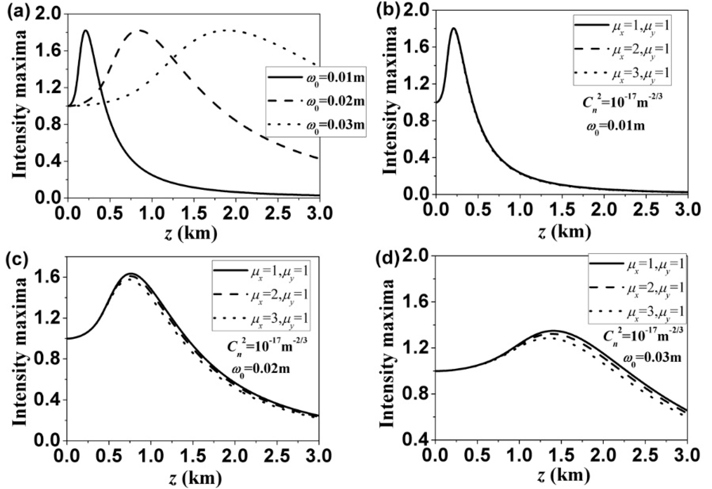
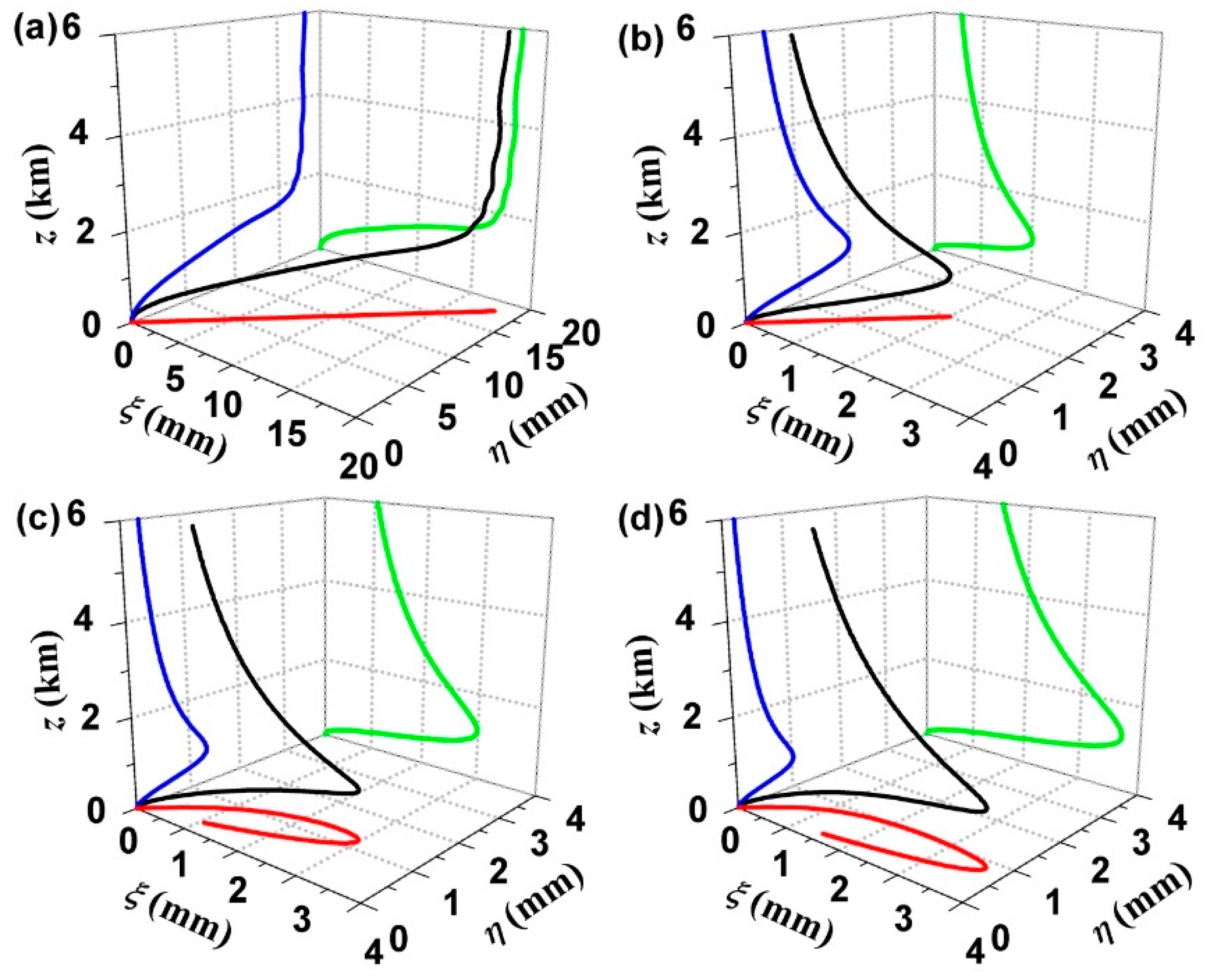
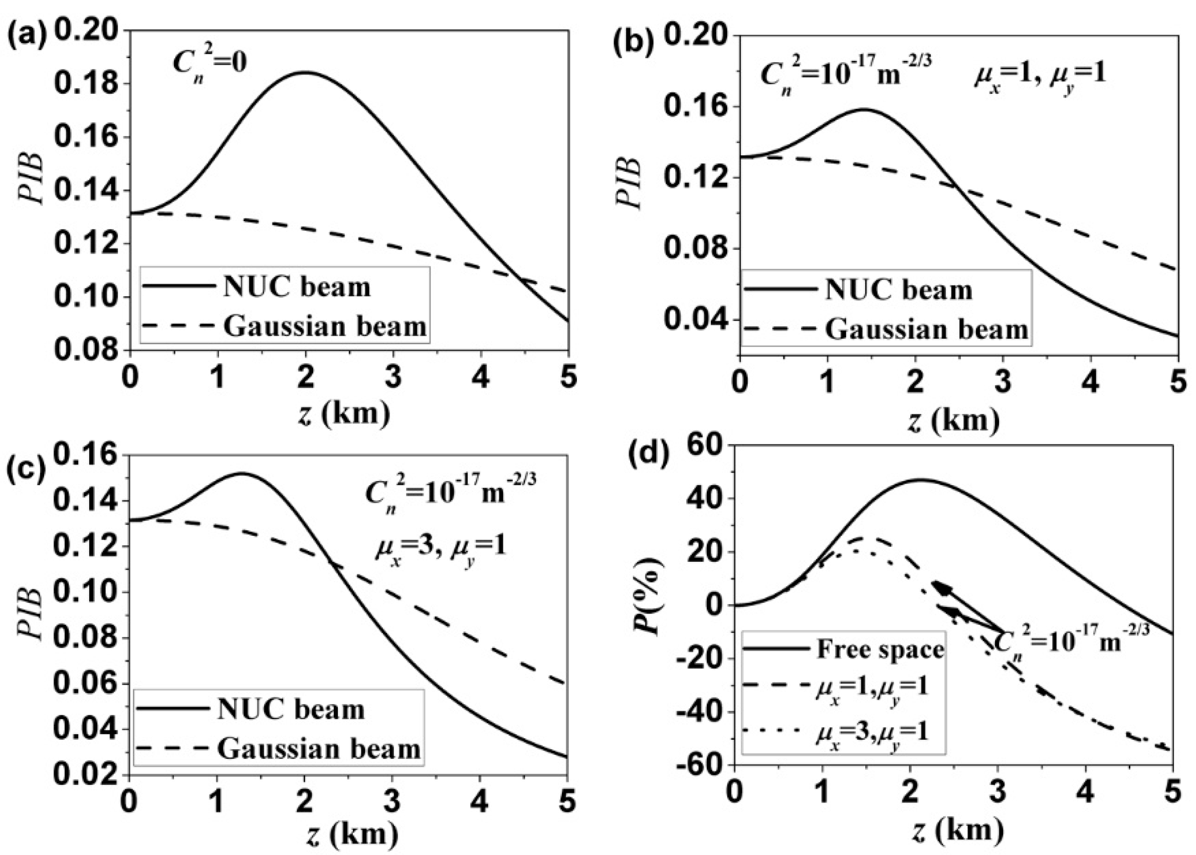
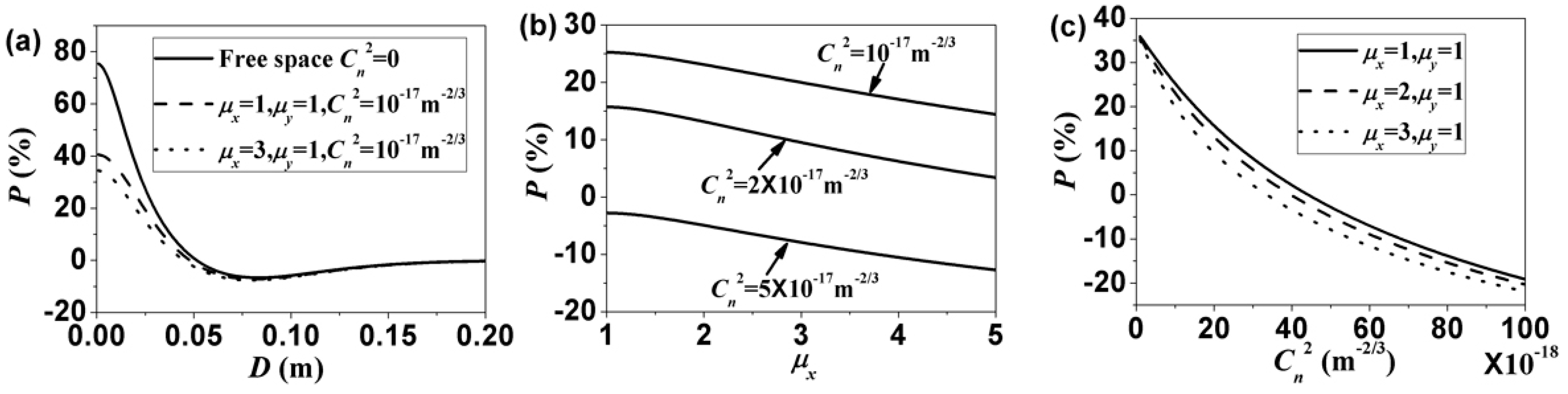
3. Propagation Characteristics of the NUC Beams in Anisotropic Turbulence Along the Horizontal Links

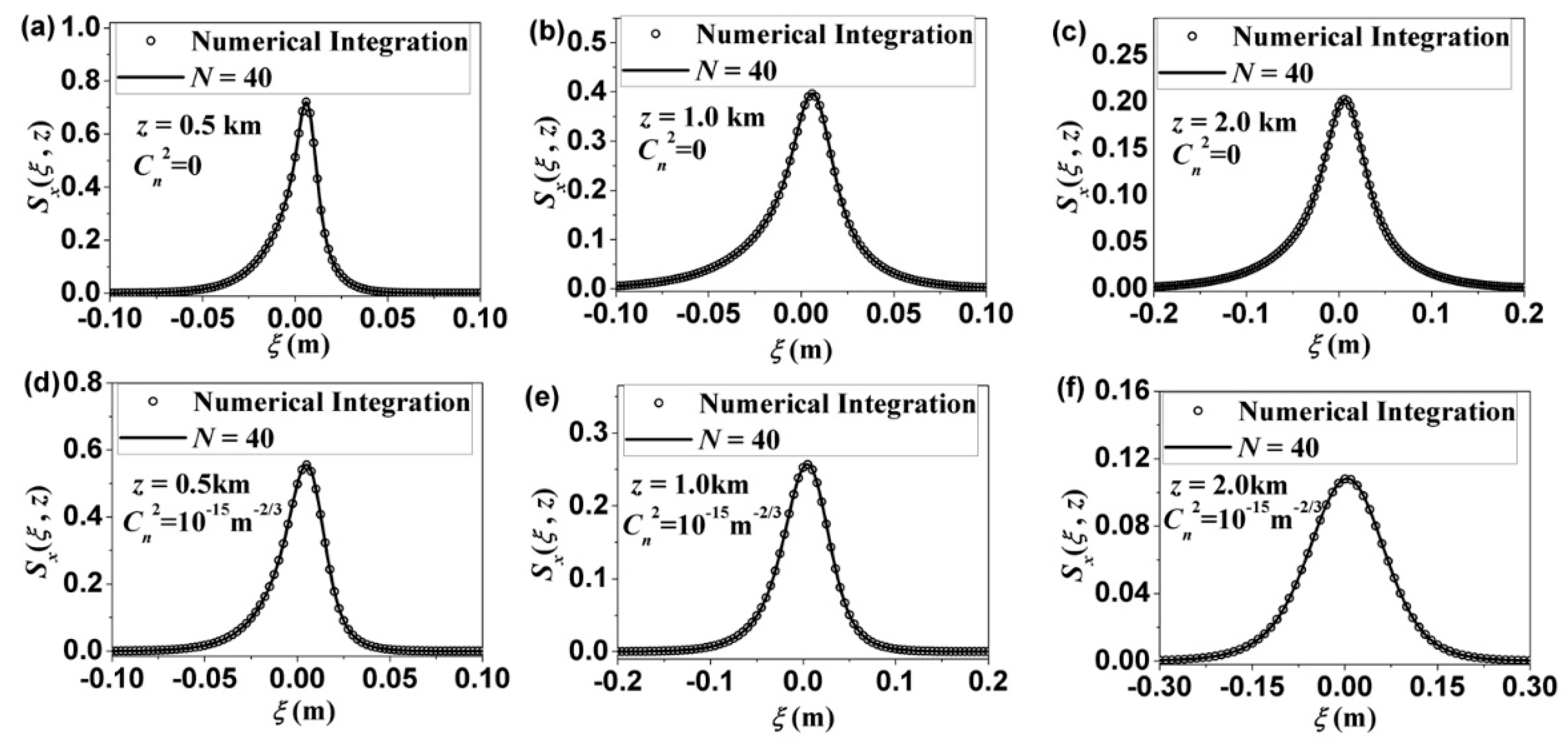
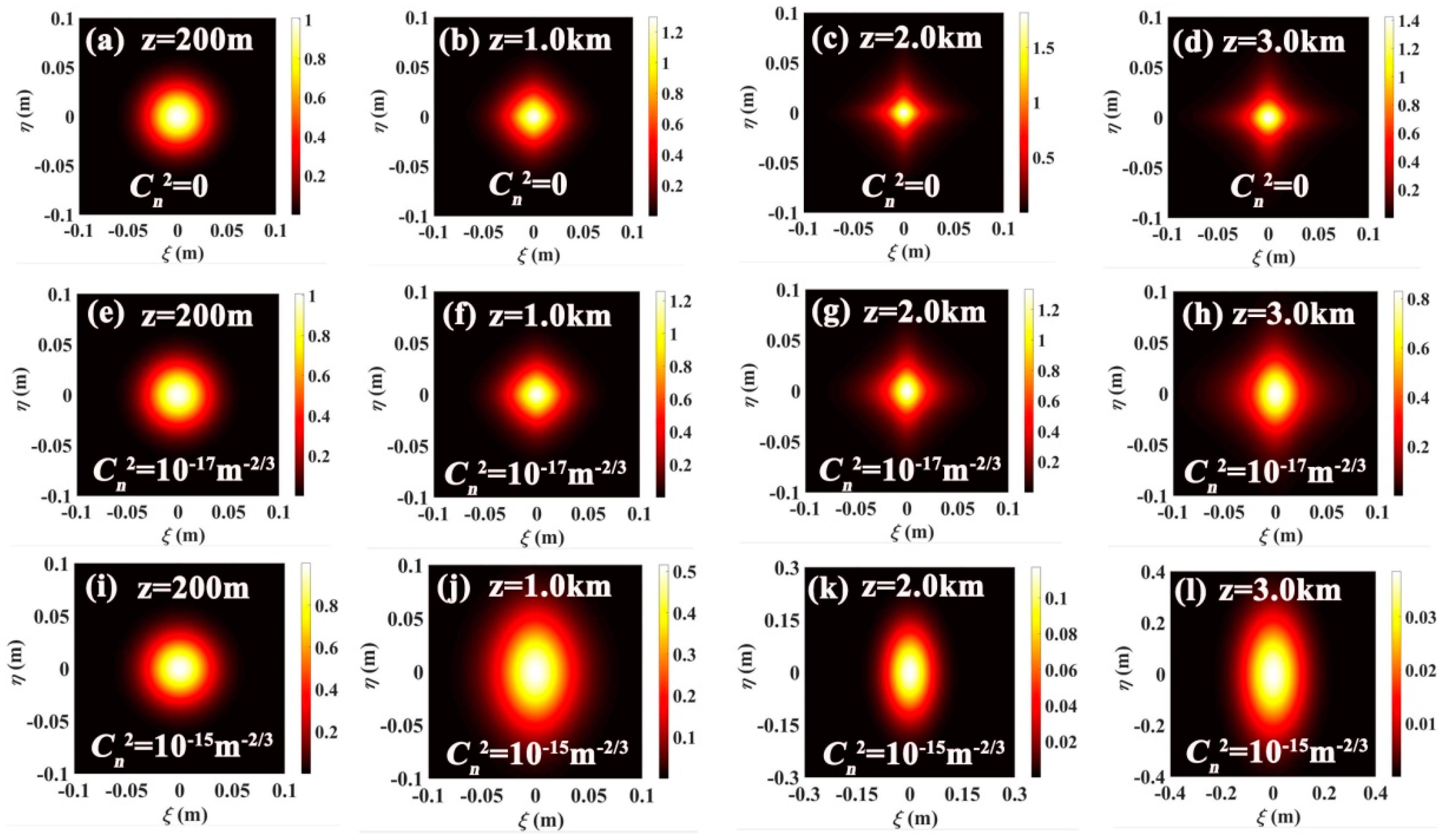
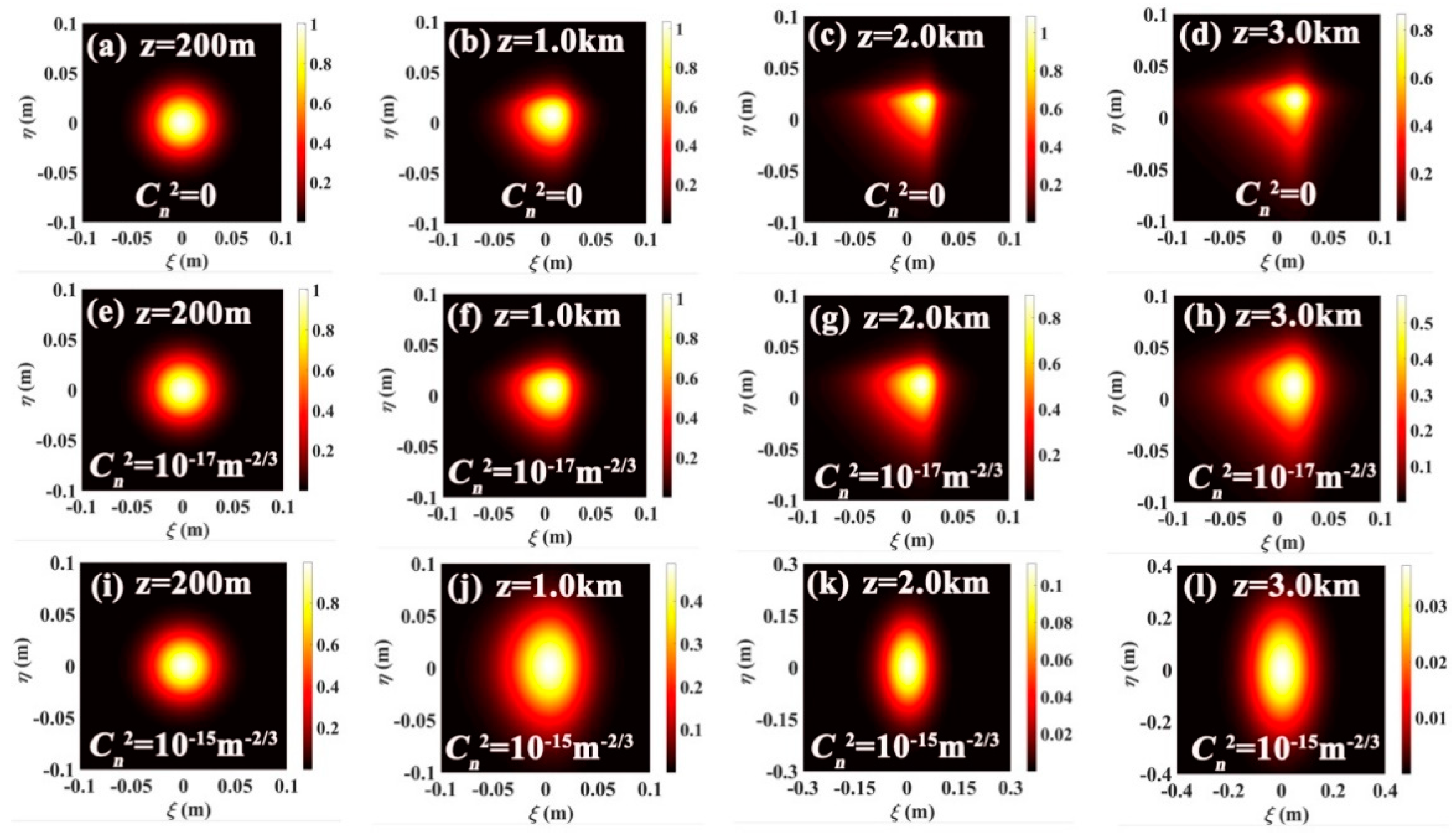
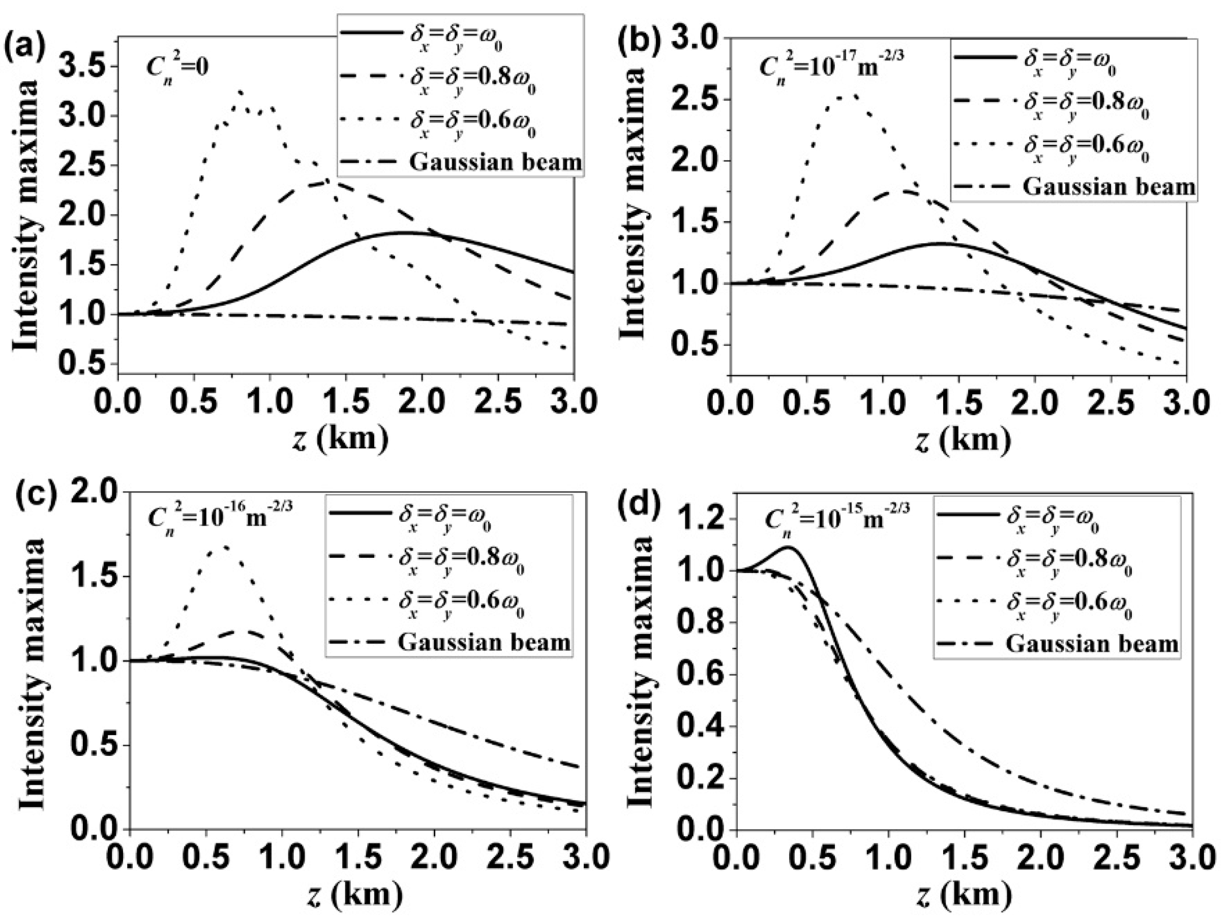
Spectral Density of the NUC Beams Propagation through Anisotropic Turbulence

According to [35], the cross-spectral density (CSD) function of the NUC beams in the source plane is represented by the following integral formula:

$$W_x(x_1,x_2)={\displaystyle \int p_x(v)H_x^{*}(x_1,v)H_x(x_2,v)dv}.$$

(7)

The functions p_x(v) and H_x(x,v) entering in Equation (7) take the form:

$$p_x(v)={(\pi a_x^2)}^{-1/2}\exp (-v^2/a_x^2),$$

(8)

$$H_x(x,v)=\exp \left(-\frac{x^2}{2w_0^2}\right)\exp [-ik{(x-x_0)}^{2}v].$$

(9)

where k = 2π/λ is the wavenumber with λ being the wavelength of a light beam; w₀ and x₀ are real constants. On substituting Equations (8) and (9) into Equation (7) and integrating over v, the expression for the CSD function of the NUC beam becomes:

$$W_x(x_1,x_2)=\exp \left(-\frac{x_1^2+x_2^2}{2w_0^2}\right)\exp \left[-\frac{{(x_2-x_0)}^2-{(x_1-x_0)}^2}{{\delta }_x^4}\right].$$

(10)

where ${\mathsf{\delta }}_{\mathrm{x}}=\sqrt{2/\mathrm{k}{\mathrm{a}}_{\mathrm{x}}}$, is the r.m.s correlation width. Please note that Equation (10) only represents the one-dimensional case for the NUC beams. The extension of the NUC beams to the two-dimensional case is straightforward, i.e., W₀(r₁,r₂) = W_x(x₁,x₂)W_y(y₁,y₂). The function W_y(y₁,y₂) is immediately derived from W_x(x₁,x₂) replacing x with y in Equation (10). r₁ ≡ (x₁,y₁) and r₂ ≡ (x₂,y₂) are two position vectors in the source plane. It can be seen that the two-dimensional CSD function is a separable function with respect to the variables (x₁,x₂) and (y₁,y₂).

In the presence of anisotropic turbulence and within the validity of the paraxial approximation, the spectral density of the NUC beams in a plane at distance z from the source plane (z = 0) can be treated by the following eHF integral

$$\begin{array}{l}S(\mathsf{\rho },z)={\left(\frac{k}{2\pi z}\right)}^2{\displaystyle {\displaystyle \int \int W_0({\mathbf{r}}_1,{\mathbf{r}}_2)\exp \left[\frac{ik}{2z}\left({\left|{\mathbf{r}}_2-\mathsf{\rho }\right|}^2-{\left|{\mathbf{r}}_1-\mathsf{\rho }\right|}^2\right)\right]}}\\ \times {\langle \exp \left({\psi }^{*}({\mathbf{r}}_1,\mathsf{\rho },z)+\psi ({\mathbf{r}}_2,\mathsf{\rho },z)\right)\rangle }_m{d}^2{\mathbf{r}}_{1}d{\mathbf{r}}_2,\end{array}$$

(11)

where ρ ≡ (ξ,η) is the position vector in the plane of z. The angular brackets with subscript m denote ensemble average over the turbulent medium. The function ψ(r,ρ,z) denotes the complex phase fluctuations of a spherical wave propagating from (r, 0) to ($\mathsf{\rho }$, $z$). According to [33], the second-order statistics of the phase correlation induced by the anisotropic turbulence can be approximately expressed by the following expression:

$$\begin{array}{l}{F}_2({\mathbf{r}}_1,{\mathbf{r}}_2,\mathsf{\rho },z)={\langle \exp \left({\psi }^{*}({\mathbf{r}}_1,\mathsf{\rho },z)+\psi ({\mathbf{r}}_2,\mathsf{\rho },z)\right)\rangle }_m\\ =\exp \left[-\frac{{\pi }^2{k}^{2}Tz}{3}\left(\frac{x_d^2}{{\mu }_x^2}+\frac{y_d^2}{{\mu }_y^2}\right)\right],\end{array}$$

(12)

with

$$\begin{array}{l}T={\displaystyle {\int }_0^{\infty }{\kappa }^{\prime }{}^3{\Phi }_n({\kappa }^{\prime })d{\kappa }^{\prime }/{\mu }_x{\mu }_y}\\ =0.0033{\mu }_z{C}_n^2\left[\Gamma \left(\frac{1}{6},\frac{{\kappa }_{eff}^2}{{\kappa }_m^2}\right)\frac{(6{\kappa }_{eff}^2+5{\kappa }_m^2)}{{\kappa }_m^{5/6}}-6{\kappa }_{eff}^{1/3}\right],\end{array}$$

(13)

where x_d = x₂− x₁ and y_d = y₂− y₁. Γ is the Gamma function. As shown in Equation (13), F₂ is also a separable function with respect to (x₁,x₂) and (y₁,y₂). Therefore, we can rewrite Equation (11) as a product of the x and y parts of the spectral density in anisotropic turbulence, i.e.,

$$S(\mathsf{\rho },z)=S_x(\xi ,z)S_y(\eta ,z),$$

(14)

with

$$\begin{array}{l}{S}_{\alpha }(\beta ,z)=\frac{k}{2\pi z}{\displaystyle \int W_{\alpha }({\alpha }_1,{\alpha }_2)\exp \left[\frac{ik}{2z}\left({\alpha }_2^2-{\alpha }_1^2\right)-\frac{ik\beta }{z}\left({\alpha }_2-{\alpha }_1\right)\right]}\\ \times \exp \left(-\frac{{\pi }^2{k}^{2}Tz{\left({\alpha }_2-{\alpha }_1\right)}^2}{3{\mu }_{\alpha }^2}\right)d{\alpha }_{1}d{\alpha }_2,(\alpha =x,y;\beta =\xi ,\eta ).\end{array}$$

(15)

In general, it is impossible to acquire the analytical expression for the spectral density from Equation (15). One approach for obtaining an approximate analytical expression is to write the integral formula [shown in Equation (7)] for the CSD function in terms of a finite number of modes, see [44]

$$W_{\alpha }({\alpha }_1,{\alpha }_2)={\displaystyle \sum _{n=1}^N{A}_n^{*}({\alpha }_1)A_n({\alpha }_2)},(\alpha =x,y),$$

(16)

with $A_n\left(\alpha \right) = \Delta v^{1/2}{p}_{\alpha }{\left(v_n\right)}^{1/2}{H}_{\alpha }\left(\alpha ,v_n\right)$. $\mathsf{\Delta }v$ is the spacing of the modes; N represents the number of the discrete modes. On substituting Equation (16) into Equation (15) and after some manipulations and integration, we obtain the approximate analytical expression for the x(y) part of the spectral density

$$\begin{array}{l}{S}_{\alpha }(\beta ,z)={\displaystyle \sum _{n=1}^N\frac{k{w}_0{\delta }_{\alpha }^2\Delta v}{2\sqrt{\pi M_{\alpha }}}\exp \left(-\frac{k^2{\delta }_{\alpha }^4{v}_n^2}{4}\right)}\\ \times \exp \left[-\frac{{\left(\beta -2z{v}_n{\alpha }_0\right)}^2}{M_{\alpha }}\right],(\alpha =x,y;\beta =\xi ,\eta ),\end{array}$$

(17)

with

$$M_{\alpha }=\frac{z^2}{k^2{w}_0^2}+\frac{4{\pi }^{2}T{z}^3}{3{\mu }_{\alpha }^2}+w_0^2{\left(1-2z{v}_n\right)}^2.$$

(18)

Equation (17) is the main result of this paper. It allows us to investigate the evolution properties of the spectral density in anisotropic turbulence conveniently. However, the accuracy of Equation (17) depends on the number of the discrete modes N and the range of the interval for |v|.

To show the accuracy of Equation (17), which is equal to the exact Equation (15) if the number of discrete modes N tends to infinity, we plot in Figure 1 the variation of the spectral density S_x(ξ,z) as a function of ξ at several propagation distances both in free space and in turbulent atmosphere. The pertinent quantities are calculated from Equation (17) (solid lines) and the direct integration of Equation (15) (circular dots). In the numerical calculation we sampled the modes in the interval |v| ≦ 2a_x. The other parameters used in the calculation are chosen to be ω₀ = 10 mm, δ_x = 10 mm, x₀ = 0.7ω₀, λ = 632.8 nm, l₀ = 0.01 m, L₀ = 1.0 m and μ_z = μ_x = μ_y = 3. It is shown that the spectral densities at three propagation distances, calculated from Equation (17) with N = 40, agree well with those calculated from direct integration, both in free space and in the presence of turbulence. However, the results obtained from Equation (17) save a lot of computation time compared to those obtained from direct integration, which means that the method for the mode decompositions is a convenient and efficient way to evaluate the spectral density of NUC beams on propagation.

Let us consider the NUC beams propagating along the horizontal path near the ground with the z axis being the main propagation direction. It is reasonable to assume that the anisotropic factor μ_x equals to μ_z and is larger than μ_y. The initial parameters used in the calculation are ω₀ = 30 mm, δ_x = δ_y = 30 mm, λ = 632.8 nm, μ_x = μ_z = 2, μ_y = 1, l₀ = 0.01 m, L₀ = 1.0 m and fixed throughout the text unless other values are specified.

Figure 2 illustrates the spectral density of the NUC beam with x₀ = 0 at different propagation distances both in free space ($C_n^2$ = 0) and in the presence of anisotropic turbulence with two different values of the constant structures $C_n^2$ = 10⁻¹⁷ m^−2/3 and $C_n^2$ = 10⁻¹⁵ m^−2/3. In free space, because of the initial state of partial coherence, the beam gradually transits from a Gaussian profile to a diamond shape as the propagation distance increases. The position of the intensity maxima keeps unchanged on propagation since the initial value of x₀ = y₀ = 0 equals zero. Please note that the maximum intensity at the transverse plane is enhanced on propagation, i.e., the values of the intensity maxima exceed one which is the maxima value in the source plane [see the color bar in Figure 2a–d]. In the presence of anisotropic turbulence, the beam profile loses its diamond shape, and changes into an elliptical shape in the far field [see in Figure 2h,l]. When the strength of turbulence increases, the beam profile turns into an elliptical shape at a relative short distance [seen in Figure 2i–l] and keeps its elliptical shape on further propagation. The maximum intensity (on-axis point) is greatly suppressed owing to the effects of turbulence. As shown Equation (12), (i.e., the second-order statistics of phase correlation), the effect of turbulence on the beam propagation is that it looks like imposing an elliptical Gaussian-Schell-model term on the beam. However, when the propagation distance is short, or the turbulence is weak, the parameter T in Equation (12) is very small. Hence the turbulence effect can then be neglected. In this case, the beam profile keeps its free-space features. When the propagation distance is large enough, or the turbulence is strong, the situation is reversed. The effect of turbulence dominates the central role to determine the beam profile and turns the beam profile into an elliptical shape. In our numerical examples, the anisotropy factor in x direction is larger than that in the y direction, implying that the strength of the turbulence in the y direction is much stronger. Thus, the spectral density of the NUC beams are elongated along the y-axis. Here, we should emphasize that the turbulence we consider belongs to weak turbulence. According to [1], a widely used parameter to judge whether the turbulence is weak is the Rytov variance, defined as ${\sigma }_R^2=1.23C_n^2{k}^{7/6}{z}^{11/6}$. If ${\sigma }_R^2<1$, the turbulence is weak. In our numerical examples, when the propagation distance is z = 3.0 km, the calculated values of the parameter is about 0.004 and 0.4 for $C_n^2$ = 10⁻¹⁷ m^−2/3 and $C_n^2$ = 10⁻¹⁵ m^−2/3, respectively.

Figure 3 shows the spectral density of the NUC beam with x₀ = y₀ = 0.7ω₀ at four different propagation distances in free space and in the presence of anisotropic turbulence. In the case of free space, the beam profile gradually turns into a sector-like shape during free-space propagation and lateral shifting of the intensity maxima occurs, which is much different from those with x₀ = y₀ = 0 [see Figure 2a–d and Figure 3a–d]. It is shown in Figure 3e–l that the spectral density is strongly affected by anisotropic turbulence, especially for $C_n^2$ = 10⁻¹⁵ m^−2/3, i.e., the evolution of the spectral density for x₀ = y₀ = 0.7ω₀ is quite similar to that of the NUC beam for x₀ = y₀ = 0. This phenomenon can be explained by the fact that there are two factors determining the evolution of the spectral density with the propagation distance. One is the initial correlation properties of the field, and the other one is the effect of turbulence. When the turbulence is weak, or the propagation distance is short, the former factor determines the feature of the spectral density. When the turbulence is relative strong, or the propagation distance is long enough, the latter factor plays a central role in determining the evolution properties of the spectral density. Therefore, the evolution properties of the NUC beams between x₀ = y₀ = 0 and x₀ = y₀ = 0.7ω₀ are almost the same when $C_n^2$ = 10⁻¹⁵ m^−2/3.

Figure 4 illustrates the evolution of the on-axis intensity (intensity maxima) of the NUC beams (x₀ = y₀ = 0) with different values of coherence widths as a function of the propagation distance z in free space and in the presence of anisotropic turbulence. For comparison, the variation of the on-axis intensity of the fundamental Gaussian beam (dash-dot lines) with the propagation distance is also plotted in Figure 4. In the calculation, the initial beam width of the Gaussian beam is the same as that of the NUC beams. One finds that the value of the on-axis intensity of the NUC beams exceeds that in the source plane during free-space propagation, implying that a sharpened intensity distribution occurs. For NUC beams with large values of the coherence width the sharpened intensity distribution can last for long propagation distances, compared to those with smaller values of the coherence width. However, the maximum value decreases as the coherence width increases. Please note that after reaching the maximum value, the on-axis intensity decays much faster than that of the Gaussian beam when the propagation distance increases further. In the presence of turbulence, the sharpened intensity distribution of the NUC beams is strongly affected by the strength of the turbulence. The propagation distance, which retains the sharpened intensity, is greatly shortened, compared to the case in free space. When the strength of the turbulence is $C_n^2$ = 10⁻¹⁵ m^−2/3, the NUC beams with three values of coherence width almost have the same values for the on-axis intensity. These values of the on-axis intensity are much lower than those for a Gaussian beam with a propagation distance larger than 600 m [see in Figure 4d].

Figure 5 gives the variation of the on-axis intensity of the NUC beams (x₀ = y₀ = 0) with ω₀ = 0.01 m, 0.02 m, and 0.03 m as a function of the propagation distance in free space and in the presence of anisotropic turbulence with different anisotropy factors. One can see in Figure 5a that for different initial beam sizes the maximum values of the on-axis intensity are the same. However, the propagation distance for which the maximum intensity occurs is closely related to the initial beam size. The larger the values of the initial beam size, the longer the propagation distances needed for obtaining the maximum intensity. In turbulence with different anisotropy factors [see in Figure 5b–d], it can be seen that as the anisotropy factor μ_x increases, the values of the on-axis intensity of the NUC beams with larger beam size decrease more rapidly. From Figure 4 and Figure 5, one may also conclude that the NUC beams still have the ability to retain the sharpened intensity distribution in atmospheric turbulence when the structure constant $C_n^2$ is smaller than 10⁻¹⁶ m^−2/3. One can modulate the initial beam size or coherence width to acquire the maximum intensity at the receiver plane. This maximum intensity may even be higher than that of the Gaussian beam under the same condition. This peculiar property of the maximum intensity is quite useful for an information carrier in free space. The anisotropy factors also have the additional effects to affect the evolution of the on-axis intensity.

If the parameters x₀ and y₀ of the NUC beams are not zero, the position of the intensity maxima will shift laterally from the on-axis point upon free-space propagation due to the non-uniform source correlations. To examine the behavior of the lateral shifting in the presence of anisotropic turbulence, we plot in Figure 6 the 3D-graphs of the position of the intensity maxima (black lines) both in free space and in the presence of turbulences with different anisotropy factors. The red, green, and blue lines in Figure 6 denote the projection of the black lines in the ξ-η, ξ-z and η-z planes, respectively. In free space, the lateral shift of the intensity maxima first increases with the increase of the propagation distance, and then keeps a fixed value almost unchanged upon propagation. The shifts along the x and y direction are the same because we set the initial parameter x₀ equals to y₀ in the calculation. In the case of isotropic turbulence [see in Figure 6b], the effect of the turbulence is to suppress the shift of the intensity maxima, which is consistent with the analysis in [36]. Please note that the shifts along the x and y direction are the same, as expected. In the case of anisotropic turbulence [see in Figure 6c,d], the projection of the trace in the ξ-η plane becomes a curved line instead of a line, as in the case of isotropic turbulence. This indicates that the traces of the lateral shifts of the intensity maxima are not lying in an arbitrary plane. In our numerical case (μ_x > μ_y), the strength of the turbulence in the x(ξ) direction is weaker than that in the y(η) direction. Therefore, the lateral shift in the x(ξ) direction is always larger than that in the corresponding y(η) direction.

In a practical situation one is concerned about the amount of energy carried by the beam received by a detector in the receiver plane. The more energy the detector receives, the higher the efficiency of the optical system. However, the receiver’s aperture has finite dimensions in a practical system. Consequently, a beam whose intensity is concentrated on a small region during propagation has a certain ability to improve the energy receiving rate. Based on the previous analysis, the NUC beams may have a higher receiving energy rate, even compared to the Gaussian beam under the same conditions. Let us consider such an optical system for free-space optical communication. A laser beam, which is acting as an information carrier, is sent to the receiver via an atmospheric channel. The receiver lens collects a portion of the transmitted optical field, which is focused onto a photodetector. This portion is used to convert the optical information into electrical signals for processing.

Assume that the aperture of the receiver lens has a square shape for simplicity. Therefore, the ratio of the beam power captured by the photodetector and the total power carried by the beam, known as power-in-the-bucket (PIB), can be expressed as

$$PIB=\frac{{\displaystyle {\int }_{-D/2}^{D/2}{\displaystyle {\int }_{-D/2}^{D/2}S(\xi ,\eta ,z)d\xi d\eta }}}{{\displaystyle \int {\displaystyle \int S(\xi ,\eta ,z)d\xi d\eta }}},$$

(19)

where D is the width of the square aperture of the lens. By inserting Equation (17) into (19) and after integrating over ξ and η, we can obtain the analytical expression for the PIB:

$$PIB=\frac{p_x(D)p_y(D)}{\pi w_0^2},$$

(20)

with

$$\begin{array}{l}{p}_{\alpha }={\displaystyle \sum _{n=1}^N\frac{k{w}_0{\delta }_{\alpha }^2\Delta v}{4}\exp \left(-\frac{k^2{\delta }_{\alpha }^4{v}_n^2}{4}\right)}[Erf\left(\frac{2z{v}_n{\alpha }_0+D/2}{\sqrt{M_{\alpha }}}\right)\\ -Erf\left(\frac{2z{v}_n{\alpha }_0-D/2}{\sqrt{M_{\alpha }}}\right)],(\alpha =x,y)\end{array}$$

(21)

where Erf denotes the error function.

The dependence of the PIB of the NUC beam (x₀ = y₀ = 0) on the propagation distance in free space, in the presence of isotropic turbulence or anisotropic turbulence, is shown in Figure 7a–c. The size of the aperture D used in the calculation is 0.04 m. For comparison, the corresponding results of the PIB of the Gaussian beam which have the same initial beam width as the NUC beam (ω₀ = 30 mm), are also plotted in Figure 7a–c (dashed lines). It is shown that the PIB of the NUC beam is larger than that of the Gaussian beam under the same condition on free-space propagation from the source z = 0 to a distance of 3 km away from it. This means that more power will be received by the detector if illuminated by the NUC beam. However, this advantage is weakened or disappears in the presence of turbulence, be it isotropic or anisotropic turbulence.

As shown in Figure 7b, the advantage of the NUC beam is only in the region 0–2.5 km. The PIB of the NUC beam drops rather quickly when the propagation distance is larger than 1.5 km. In the case of anisotropic turbulence, the situation becomes worse. It only keeps its superior behavior for propagation distances less than 2.0 km [see in Figure 7c]. Our other numerical results (not shown here) indicate that when the strength of turbulence is larger than 10⁻¹⁵ m^−2/3, the NUC beam will lose its advantages. To quantitatively assess the superiority of the NUC beam, compared to the Gaussian beam, the following parameter is introduced to characterize it, i.e.,

$$P=\frac{PI{B}_{NUC}-PI{B}_{Gau}}{PI{B}_{Gau}}.$$

(22)

In Equation (22), the PIB with the subscript “NUC” and “Gau” denote the power-in-bucket of NUC beams and Gaussian beams, respectively. The positive of P means the NUC beams are superior to the Gaussian beams. Figure 7d shows the variation of P against the propagation distance both in free space and in the presence of atmospheric turbulence. One can see that the maximum value of P is about 25% or 20% near the propagation distance z = 1.5 km in the case of isotropic or anisotropic turbulence, respectively.

Figure 8 illustrates the dependence of P on the width of the receiver aperture, the anisotropic factor μ_x with μ_y = 1 and D = 0.02 m, and the strength of turbulence with D = 0.02 m at z = 1.5 km. It is shown in Figure 8a that for $C_n^2$ = 10⁻¹⁷ m^−2/3 more power can be received using a NUC beam than using a Gaussian beam when the aperture is relatively small (D < 0.05 m), irrespectively of whether isotropic or anisotropic turbulence is present. However, when the aperture size is in the range of 0.05 m < D < 0.15 m, the situation is reversed, i.e., the detector could receive more beam energy using the Gaussian beam. If the aperture size increases further, there is almost no discrepancy between the Gaussian beam and the NUC beam because all the power carried by the beams is captured by the detector. Figure 8b clearly shows that the increase of the anisotropic factor μ_x leads to the reduction of the advantage of the NUC beam. Figure 8c indicates that only if the structure constant $C_n^2$ is smaller than approximately 3 × 10⁻¹⁷ m^−2/3, a higher part of the power of the NUC beam can be received in the output plane, compared to that of the Gaussian beam.

4. Conclusions

We have studied the average intensity, lateral shift of the intensity maxima and the PIB in the receiver plane in the case of NUC beams endowed with a rectangular symmetry. The beams propagate through free space or in the presence of either isotropic- or anisotropic turbulence. The calculations are based on the approximate analytical expression for the propagation of the spectral density derived in this paper. The beam was shown to have either a diamond profile for x₀ = y₀ = 0 or a sector-like profile for x₀ = y₀ > 0 in the far field on free-space propagation. Even though on the propagation in the presence of anisotropic turbulence the NUC beams still can keep its diamond or sector-like shape in a weak turbulence regime, they will degenerate to an elliptical shape in moderate or strong turbulence. The evolution of locally sharpened and locally shifted intensity maxima is closely related to the strength of the turbulence and the anisotropic coefficients. The sharpened intensity maxima decrease gradually and disappear finally with increasing strength of the turbulence. In addition, the behavior of the PIB of the NUC beams and the Gaussian beam with the same initial beam width for both isotropic and anisotropic beams has been compared. Our results show that the PIB of the NUC beam can be even higher than that of the Gaussian beam in the presence of a very weak turbulence regime. In free-space optical (FSO) communications, the average receiving energy (ARE) is one of the important factors affecting optical communication. High ARE is preferred in FSO communications; however, a light beam propagating through the atmosphere is subject to phase fluctuations due to atmospheric turbulence, which causes the extra beam spreading beyond the spread due to the diffraction. This effect will reduce the ARE in the receiver plane. The NUC beams exhibit the higher PIB propagation in turbulence under certain conditions. We believe that this propagation feature of the NUC beams may have important applications in FSO communication and remote sensing.

References

1. Andrews, L.C.; Phillips, R.L. Laser Beam Propagation through Random Medium, 2nd ed.; SPIE Press: Bellingham, WA, USA, 2005; ISBN 9780819459480. [Google Scholar]
2. Consortini, A.; Ronchi, L.; Stefanutti, L. Investigation of Atmospheric Turbulence by Narrow Laser Beams. Appl. Opt. 1970, 9, 2543–2547. [Google Scholar] [CrossRef] [PubMed]
3. Dalaudier, F.; Sidi, C.; Crochet, M.; Vernin, J. Direct evidence of “sheets” in the atmospheric temperature field. J. Atmos. Sci. 1994, 51, 237–248. [Google Scholar] [CrossRef]
4. Grechko, G.M.; Gurvich, A.S.; Kan, V.; Kireev, S.V.; Savchenko, S.A. Anisotropy of spatial structures in the middle atmosphere. Adv. Space Res. 1992, 12, 169–175. [Google Scholar] [CrossRef]
5. Robert, C.; Conan, J.M.; Michau, V.; Renard, J.B.; Dalaudier, F. Retrieving parameters of the anisotropic refractive index fluctuations spectrum in the stratosphere from balloon-borne observations of stellar scintillation. J. Opt. Soc. Am. A 2008, 25, 379–393. [Google Scholar] [CrossRef]
6. Antoshkin, L.V.; Botygina, N.N.; Emaleev, O.N.; Lavrinova, L.N.; Lukin, V.P.; Rostov, A.P.; Fortes, B.V.; Yankov, A.P. Investigation of turbulence spectrum anisotropy in the ground atmospheric layer, preliminary results. Atmos. Ocean. Opt. 1995, 8, 993–996. [Google Scholar]
7. Manning, R.M. An anisotropic turbulence model for wave propagation near the surface of the Earth. IEEE Trans. Antennas Propag. 1986, AP-34, 258–261. [Google Scholar] [CrossRef]
8. Biferale, L.; Procaccia, I. Anisotropic contribution to the statistics of the atmospheric boundary layer. Phys. Rep. 2005, 414, 43–164. [Google Scholar] [CrossRef]
9. Belen’kii, M.S.; Barchers, J.D.; Karis, S.J.; Osmon, C.L.; Brown, J.M., II; Fugate, R.Q. Preliminary experimental evidence of anisotropy of turbulence and the effect of non-Kolmogorov turbulence on wavefront tilt statistics. Proc. SPIE 1999, 3762, 396–406. [Google Scholar] [CrossRef]
10. Belen’kii, M.S.; Karis, S.J.; Osmon, C.L. Experimental evidence of the effects of non-Kolmogorov turbulence and anisotropy of turbulence. Proc. SPIE 1999, 3749, 50–51. [Google Scholar] [CrossRef]
11. Gladkikh, V.A.; Nevzorova, I.V.; Odintsov, S.L.; Fedorov, V.A. Turbulence anisotropy in the near-ground atmospheric layer. Proc. SPIE 2014, 9292, 92925F-1. [Google Scholar] [CrossRef]
12. Funes, G.; Olivares, F.; Weinberger, C.G.; Carrasco, Y.D.; Nunez, L.; Perez, D.G. Synthesis of anisotropic optical turbulence at the laboratory. Opt. Lett. 2016, 41, 5696–5699. [Google Scholar] [CrossRef] [PubMed]
13. Bos, J.P.; Roggemann, M.C.; Gudimetla, V.S.R. Anisotropic non-Kolmogorov turbulence phase screens with variable orientation. Appl. Opt. 2015, 54, 2039–2045. [Google Scholar] [CrossRef] [PubMed]
14. Wheelon, A.D. Electromagnetic Scintillation I. Geometric Optics; Cambridge University Press: Boulder, CO, USA, 2001; ISBN 9780521020121. [Google Scholar]
15. Toselli, I. Introducing the concept of anisotropy at different scales for modeling optical turbulence. J. Opt. Soc. Am. A 2014, 31, 1868–1875. [Google Scholar] [CrossRef] [PubMed]
16. Rao Gudimetla, V.S.; Holmes, R.B.; Smith, C.; Needham, G. Analytical expressions for the log-amplitude correlation function of a plane wave through anisotropic atmospheric refractive turbulence. J. Opt. Soc. Am. A 2012, 29, 832–841. [Google Scholar] [CrossRef] [PubMed]
17. Rao Gudimetla, V.S.; Holmes, R.B.; Riker, J.F. Analytical expressions for the log-amplitude correlation function for plane wave propagation in anisotropic non-Kolmogorov refractive turbulence. J. Opt. Soc. Am. A 2012, 29, 2622–2627. [Google Scholar] [CrossRef] [PubMed]
18. Rao Gudimetla, V.S.; Holmes, R.B.; Riker, J.F. Analytical expressions for the log-amplitude correlation function for spherical wave propagation through anisotropic non-Kolmogorov atmosphere. J. Opt. Soc. Am. A 2014, 31, 148–154. [Google Scholar] [CrossRef] [PubMed]
19. Cui, L. Analysis of temporal power spectra for optical waves propagating through weak anisotropic non-Kolmogorov turbulence. J. Opt. Soc. Am. A 2015, 32, 1199–1208. [Google Scholar] [CrossRef] [PubMed]
20. Cui, L.; Xue, B. Influence of asymmetry turbulence cells on the angle of arrival fluctuations of optical waves in anisotropic non-Kolmogorov turbulence. J. Opt. Soc. Am. A 2015, 32, 1691–1699. [Google Scholar] [CrossRef] [PubMed]
21. Cui, L.; Xue, B. Influence of anisotropic turbulence on the long-range imaging system by the MTF model. Infrared Phys. Technol. 2015, 72, 229–238. [Google Scholar] [CrossRef]
22. Cui, L. Analysis of angle of arrival fluctuations for optical wave’s propagation through weak anisotropic non-Kolmogorov turbulence. Opt. Express 2015, 23, 6313–6325. [Google Scholar] [CrossRef] [PubMed]
23. Toselli, I.; Agrawal, B.; Restaino, S. Light propagation through anisotropic turbulence. J. Opt. Soc. Am. A 2011, 28, 483–488. [Google Scholar] [CrossRef] [PubMed]
24. Toselli, I.; Korotkova, O. Spread and wander of a laser beam propagating through anisotropic turbulence. Proc. SPIE 2015, 9614, 96140B. [Google Scholar] [CrossRef]
25. Toselli, I.; Korotkova, O. General scale-dependent anisotropic turbulence and its impact on free space optical communication system performance. J. Opt. Soc. Am. A 2015, 32, 1017–1025. [Google Scholar] [CrossRef] [PubMed]
26. Andrews, L.C.; Phillips, R.L.; Crabbs, R.; Leclerc, T. Deep turbulence propagation of a Gaussian-beam wave in anisotropic non-Kolmogorov turbulence. Proc. SPIE 2013, 8874, 887402. [Google Scholar] [CrossRef]
27. Yao, M.; Toselli, I.; Korotkova, O. Propagation of electromagnetic stochastic beams in anisotropic turbulence. Opt. Express 2014, 22, 31608–31619. [Google Scholar] [CrossRef] [PubMed]
28. Wang, J.; Zhu, S.; Wang, H.; Cai, Y.; Li, Z. Second-order statistics of a radially polarized cosine-Gaussian correlated Schell-model beam in anisotropic turbulence. Opt. Express 2016, 24, 11627–11639. [Google Scholar] [CrossRef] [PubMed]
29. Zhi, D.; Tao, R.; Zhou, P.; Ma, Y.; Wu, W.; Wang, X.; Si, L. Propagation of ring Airy Gaussian beams with optical vortices through anisotropic non-Kolmogorov turbulence. Opt. Commun. 2017, 387, 157–165. [Google Scholar] [CrossRef]
30. Li, Y.; Zhang, Y.; Zhu, Y.; Chen, M. Effects of anisotropic turbulence on average polarizability of Gaussian Schell-model quantized beams through ocean link. Appl. Opt. 2016, 55, 5234–5239. [Google Scholar] [CrossRef] [PubMed]
31. Gbur, G. Partially coherent beam propagation in atmospheric turbulence [Invited]. J. Opt. Soc. Am. A 2014, 31, 2038–2045. [Google Scholar] [CrossRef] [PubMed]
32. Wang, F.; Liu, X.; Cai, Y. Propagation of partially coherent beam in turbulent atmosphere: A Review. Prog. Electromagn. Res. 2015, 150, 123–143. [Google Scholar] [CrossRef]
33. Wang, F.; Korotkova, O. Random optical beam propagation in anisotropic turbulence along horizontal links. Opt. Express 2016, 24, 24422–24434. [Google Scholar] [CrossRef] [PubMed]
34. Wang, F.; Toselli, I.; Li, J.; Korotkova, O. Measuring anisotropy ellipse of atmospheric turbulence by intensity correlations of laser light. Opt. Lett. 2017, 42, 1129–1132. [Google Scholar] [CrossRef] [PubMed]
35. Lajunen, H.; Saastamoinen, T. Propagation characteristics of partially coherent beams with spatially varying correlations. Opt. Lett. 2011, 36, 4104–4106. [Google Scholar] [CrossRef] [PubMed]
36. Tong, Z.; Korotkova, O. Nonuniformly correlated light beams in uniformly correlated media. Opt. Lett. 2012, 37, 3240–3242. [Google Scholar] [CrossRef] [PubMed]
37. Gu, Y.; Gbur, G. Scintillation of nonuniformly correlated beams in atmospheric turbulence. Opt. Lett. 2013, 38, 1395–1397. [Google Scholar] [CrossRef] [PubMed]
38. Tong, Z.; Korotkova, O. Electromagnetic nonuniformly correlated beams. J. Opt. Soc. Am. A 2012, 29, 2154–2158. [Google Scholar] [CrossRef] [PubMed]
39. Mei, Z.; Tong, Z.; Korotkova, O. Electromagnetic non-uniformly correlated beams in turbulent atmosphere. Opt. Express 2012, 20, 26458–26463. [Google Scholar] [CrossRef] [PubMed]
40. Jia, X.; Tang, M.; Zhao, D. Propagation of electromagnetic non-uniformly correlated beams in the oceanic turbulence. Opt. Commun. 2014, 331, 1–5. [Google Scholar] [CrossRef]
41. Tang, M.; Zhao, D. Effects of astigmatism on spectra and polarization of aberrant electromagnetic nonuniformly correlated beams in turbulent ocean. Appl. Opt. 2014, 53, 8111–8115. [Google Scholar] [CrossRef] [PubMed]
42. Hyde, M.W., IV; Bose-Pillai, S. Generation of vector partially coherent optical sources using phase-only light modulators. Phys. Rev. Appl. 2016, 6, 064030. [Google Scholar] [CrossRef]
43. Kiethe, J.; Heuer, A.; Jechow, A. Second-order coherence properties of amplified spontaneous emission from a high-power tapered superluminescent diode. Laser Phys. Lett. 2017, 14, 086201. [Google Scholar] [CrossRef] [Green Version]
44. Gu, Y.; Gbur, G. Scintillation of pseudo-Bessel correlated beams in atmospheric turbulence. J. Opt. Soc. Am. A 2010, 27, 2621–2629. [Google Scholar] [CrossRef] [PubMed]
Figure 1. Variation of spectral density S x ( ξ , z ) with ξ at three different propagation distances in free space (ac) and in the presence of turbulence (df). The solid lines are calculated from the approximate analytical formula shown in Equation (17). The circular dots are the numerical integration directly from Equation (15). It shows that irrespective of propagation in free space or in turbulence, the spectral density obtained from the approximate analytical formula Equation (17) is consistent with that obtained from direct numerical integration.
Applsci 08 02025 g001
Figure 2. Density plots of the spectral density of the NUC beam with x0 = y0 = 0 propagation through free space and in the presence of anisotropic turbulence at several different propagation distances.
Applsci 08 02025 g002
Figure 3. Density plots of spectral density of the NUC beam with x0 = y0 = 0.7ω0 in free space and in anisotropic turbulence at different propagation distances.
Applsci 08 02025 g003
Figure 4. Evolution of intensity maxima of the NUC beams (x0 = y0 = 0) as a function of propagation distance in the presence of anisotropic turbulence with different strengths of the turbulences, (a)   C n 2 = 0, (b) C n 2 = 10 17 m 2 / 3 , (c) C n 2 = 10 16 m 2 / 3 , (d) C n 2 = 10 15 m 2 / 3 . The anisotropic factors in (b–d) are μx = 2, μy = 1.
Applsci 08 02025 g004
Figure 5. Variation of the intensity maxima of the NUC beams (x0 = y0 = 0) with the propagation distance in free space in (a) and in anisotropic turbulence with different anisotropic factors in (bd).
Applsci 08 02025 g005
Figure 6. 3D-plots (black lines) of the evolution of the position of the intensity maxima during propagation in free space and in the presence of atmospheric turbulence. Red, green, and blue lines are the projections in the ξ-η, ξ-z and η-z planes, respectively. (a) free space; (b) μx = 1, μy = 1; (c) μx = 2, μy = 1; (d) μx = 3, μy = 1. The parameters x0 and y0, used in the calculation, are x0 = y0 = 0.7ω0.
Applsci 08 02025 g006
Figure 7. (ac) Variation of the PIB of the NUC beam as a function of the propagation distance, (a) in free space; (b) in the presence of isotropic turbulence; (c) in the presence of anisotropic turbulence; (d) Variation of the parameter P against the propagation distance.
Applsci 08 02025 g007
Figure 8. Dependence of the parameter P on (a) the width of a receiver aperture, (b) the anisotropic factor μx with μy = 1, D = 0.02 m, (c) the strength of turbulence with D = 0.02 m.
Applsci 08 02025 g008