A Perceptual Evaluation of Individual and Non-Individual HRTFs: A Case Study of the SADIE II Database


AudioLab, Communication Technologies Research Group, Department of Electronic Engineering, University of York, York YO10 5DD, UK
*
Author to whom correspondence should be addressed.
Appl. Sci. 2018, 8(11), 2029; https://0-doi-org.brum.beds.ac.uk/10.3390/app8112029
Submission received: 14 September 2018
/
Revised: 14 October 2018
/
Accepted: 18 October 2018
/
Published: 23 October 2018
(This article belongs to the Special Issue Psychoacoustic Engineering and Applications)
Abstract
:As binaural audio continues to permeate immersive technologies, it is vital to develop a detailed understanding of the perceptual relevance of HRTFs. Previous research has explored the benefit of individual HRTFs with respect to localisation. However, localisation is only one metric with which it is possible to rate spatial audio. This paper evaluates the perceived timbral and spatial characteristics of both individual and non-individual HRTFs and compares the results to overall preference. To that end, the measurement and evaluation of a high-resolution multi-environment binaural Impulse Response database is presented for 20 subjects, including the KU100 and KEMAR binaural mannequins. Post-processing techniques, including low frequency compensation and diffuse field equalisation are discussed in relation to the 8802 unique HRTFs measured for each mannequin and 2818/2114 HRTFs measured for each human. Listening test results indicate that particular HRTF sets are preferred more generally by subjects over their own individual measurements.
1. Introduction
Spatial audio technologies are at the heart of immersive content creation for a wide range of applications from traditional film and television production through to music production [1] and soundscape design [2]. Within traditional linear post-production workflows, popular digital audio workstations are ever-increasing their multi-channel capabilities to support spatial audio formats. There is also a growing proliferation of affordable spatial microphone arrays on the market accommodating immersive content creation at a consumer level. Similarly, in game audio, tools such as Google Resonance (developers.google.com/resonance-audio) are facilitating the creation of immersive and interactive audio within game design engines such as Unity (www.unity3d.com).
In the reproduction phase, the spatial audio is delivered via a multi-channel loudspeaker array or headphones, the latter of which typically uses binaural audio rendering, the focus of this paper. To this end, the spatial audio quality of the binaural rendering is of key importance in delivering a plausible and immersive soundfield.
Binaural audio attempts to deliver the perceptual cues inherent in normal listening in an effort to render 3D soundfields at the ears of the listener. The human auditory system is derived from a pair of spaced dynamic filters whose responses are, in part, a function of the direction-of-arrival of a sound source [3]. In binaural audio, these organic inputs are simulated by means of their equivalent time and/or frequency domain filters, referred to throughout the literature as Head Related Impulse Responses (HRIRs) or Head Related Transfer Functions (HRTFs), respectively. HRTFs define the transfer function between a localised free-field anechoic source and the signals present at a listener’s tympanic membrane (ear drum) [4]. Typical features include a time delay, spectral colourations caused by the shape of the pinnae and early reflections from the shoulders and torso. Alternatively, Binaural Room Impulse Responses (BRIRs) may be considered which include environmental contributions such as wall and floor reflections [5].
A particular transfer function, , may be applied to a signal, , by means of convolution [6] such that the output, , may be written
By convolving a signal with an HRTF or BRIR and presenting the result directly to a listener’s ears (usually via headphones), a source may be simulated as if coming from the direction in which the Impulse Response (IR) was measured. The quality with which the source is rendered depends on the individual listener and the measurements used. Binaural IRs are a result of physiological features and as such are unique to an individual. Although certain characteristics may be generalised, for example, an increase in time delay as a source moves toward the contralateral hemisphere, other features such as the high frequency spectral notches caused by the pinnae are not so easily replicated.
In this paper, we use the phrase individual HRTFs to refer to the unique HRTF measurements of a particular person. We use this phrase in place of other commonly used terms (e.g., personal, personalized, individualized) in an attempt to discriminate between real-world measurements and alternative HRTF selection/optimization processes.
The use of non-individual measurements alters the way in which a person perceives a sound. However, it is unclear as to whether this could benefit a listener [7,8]. Previous studies focus extensively on the impact individual measurements have on source localisation [9,10,11,12,13,14,15] but fail to properly consider alternative perceptual implications.
Considering the ever-growing market for binaural technology, it is necessary to consider the impact of using different binaural IRs more generally and within the context of competing rendering schemes [16,17]. It is proposed in this paper that a listener’s individual measurements may not be optimal in all cases. We find that within particular measurement sets exist listening attributes that are preferable to a wide range of subjects. As a result, the use of such sets over individual measurements may improve a person’s listening experience. In this paper, we evaluate the performance of both individual and non-individual HRTFs. In a blind study, participants were asked to rate a series of mono, stereo and binaural stimuli based on four pre-defined spatial audio attributes.
To that end, we detail the measurement and post-processing of the SADIE II Database, a follow up to the original SADIE (Spatial Audio for Domestic Interactive Entertainment) database [18]. It collates over 60,000 binaural measurements taken of 20 subjects, 16 of whom partook in the listening test.
2. Spatial Audio Quality Assessment
The evaluation of spatial audio is a complex topic. One must be careful to define parameters that are descriptive enough to capture the essence of any given stimuli without overwhelming a listening test subject. It is necessary to consider many different aspects—for example, timbre, spatialization, naturalism and fidelity as well as the impact of listener preference.
In binaural audio, the addition of HRTFs can dramatically impact a signal due to the sharp peaks and notches found in their frequency response. Previous studies have tended toward HRTF evaluation via localisation tests [9,10,11]. Findings have offered conflicting results as to the performance of individual HRTFs compared to non-individual measurements. Some find clear benefits [12,13,14] whilst others show little improvement [15]. Results often depend on the inclusion of features such as head-tracking and the type of stimuli used.
More recent studies have begun to explore HRTF preference through: methods of database optimization [19]; the examination of perceptual repeatability and variability [20,21]; and the creation of global similarity metrics [22,23]. However, in each case, perceived spatial performance was used as a stand-alone metric for comparison. Impulsive or noisy stimuli was presented over a known trajectory and participants were asked to rate the spatial effectiveness of each sample. Considering a more general listening scenario, it is important to evaluate beyond just the spatial attributes of a rendered source [24]. In this paper, we wish to examine the impact of HRTF selection by the more general evaluation of spatial audio stimuli within a real-world context.
Previous work standardised attributes for the subjective assessment of sound quality in an ITU Recommendation in 2003 [25,26]. However, the recommendation lacks sufficient attributes for the assessment of spatial audio [7]. Early examples of subjective binaural evaluation [24,27] lack clarity and consider only general spatial or timbral colouration. Pulki [28] and Huopaniemi [24] introduce perception based binaural models as a measure of binaural signal quality. Similar objective metrics have been published since [29,30]. Whilst such models are useful for monitoring authenticity, they operate by comparing a test signal to a given reference signal and as such do not directly assess a listener’s Quality of Experience (QoE).
Alternative work has identified comprehensive lists of attributes tailored for the perceptual evaluation of spatial audio. Whilst the processes with which these lists were compiled vary by author, all result in a similar collection of holistic terms. A brief summary follows. Berg proposes a set of spatial attributes based on the Repertory Grid method in which subjects identify differences in triads of stimuli [31]. Koivuniemi presents a structured method for the development of any descriptive language [32]. In an example, 12 expert listeners produce an exhaustive list of eight spatial and four timbral attributes for evaluating different spatial sound reproduction systems. Lindau developed the Spatial Audio Quality Inventory (SAQI) which presents a vocabulary containing all perceptual attributes [33]. It is derived from a focus group of 21 German speaking virtual acoustics experts. Lokki focused on the acoustics of concert halls developing a broad list of attributes from the results of an individual vocabulary profiling experiment [34]. Pearce examined the search terms used in online sound effect libraries and compiled a list of the most popular discriminators [35]. Simon was a little more specific and identified eight qualities for describing the perceived differences between non-individual HRTF sets in binaural renderings [36]. He first followed an individual vocabulary profiling procedure, similar to Lokki, before refining his terms through a series of focus groups.
We evaluate the common elements of these lists to identify four discriminatory attributes to be assessed within a listening test (see Table 1).
Given that a small number of participants was used (those measured for the SADIE II database), the contribution from each subject was significant and an exhaustive list of attributes would have been an onerous task for each subject, potentially creating a detrimental effect on the results due to listening fatigue. To avoid this, a smaller selection of attributes was used and participants were encouraged to think more carefully about the ratings given to each stimuli. Four attributes were selected to be compatible with the interface used by the participants to rate the stimuli, discussed in Section 4.
Koivuniemi [32], Lindau [33], Lokki [34], Pearce [35] and Simon [36] all identify brightness (/darkness) as the abundance of high (/low) frequencies. We use the same definition. A term to describe a sense of fullness is also included by each author. It is described as immersion by Simon and presence by Lindau. In this paper, we use the term richness (as in [32]). We describe it as the sense of a full and well balanced mix inclusive of all frequencies and with no obvious boosts or cuts.
Regarding spatial attributes, externalisation is identified by Simon, Lindau, Koivuniemi and Berg [31]. We use this term and describe it specifically as the locatedness of sources to distant points in space. An overall feeling of realism or naturalness, is also identified by the same authors. We summarize these sensations with the term preference, implying an overall plausibility of the sound field.
3. SADIE II Binaural Database
3.1. Data Summary
In order to assess the perceptual quality of individual and non-individual HRTFs, a database of individual measurements was required. To benefit future work and to be compatible with popular binaural renderers, spatially regular Ambisonic configurations were prioritised. Ambisonics has proven to be a popular workflow for binaural rendering [37,38] and as such it is favourable to contribute data to the field. Although not pertinent to this study, BRIRs are also presented in this paper for completeness.
Alternative human HRTF databases suffer from a lack of measurements made at low elevations and a limited overall resolution (see Table 2).
Measurements of dummy heads are more readily available [43,44], however, are of course by nature less applicable to individual HRTF experimentation. The SADIE II Database includes measurements down to an elevation of −81° and provides a minimum of 2114 measurements for each human subject.
The following measurements were taken of 31 subjects (22 male, 5 female, 2 non-binary, 2 dummy mannequins, ages: 20–63 (majority 20–30)) with normal hearing:
- HRTFs of a fixed latitude-longitude distribution [45],
- HRTFs of 14 key Ambisonic loudspeaker configurations (listed in Section 3.2.1),
- BRIRs of a 50 point Lebedev Grid [46],
- Headphone IR of Beyerdynamic DT990s (+ Headphone EQ filter).
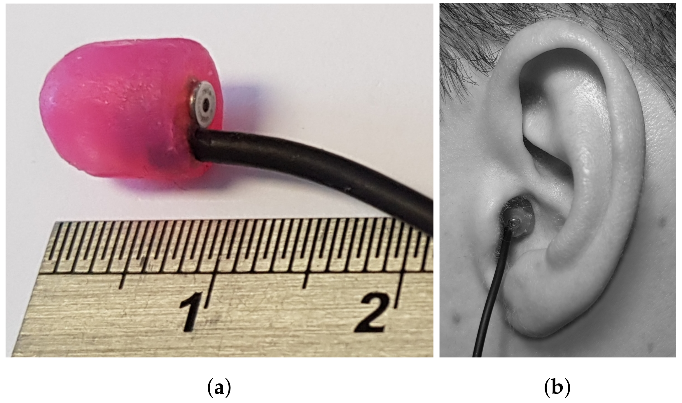
In the case of the KU100 and KEMAR mannequins, recordings were made using their built in microphones. For human subjects, a pair of Knowles FG-23329-C05 microphones (Knowles Electronics. Itasca, IL, USA.) were used and a blocked meatus approach was taken [4]. The microphones were mounted inside 3D printed capsules and secured in the participants’ ears with silicon putty (see Figure 1).
Once inserted, the microphones were not removed or re-positioned until all audiological measurements had been completed.
Twenty subjects were admitted to the final database (15 male, 1 female, 2 non-binary, 2 dummy mannequins, ages: 20–63 (majority 20–30)). Inclusion was subject to the quality of their measurements determined by observational notes and analysis of spectral, Interaural Time Difference (ITD) and Interaural Level Difference (ILD) plots. One subject voluntarily stopped the measurement procedure part way though. Six subjects were excluded due to excessive movement and shuffling in-between measurements. Two subjects were excluded due to minor asymmetries in their ITD plots. Two subjects were excluded due to unexplained discontinuities in their measurements, possibly a result of movement. Qualifying datasets included those of the KU100 dummy head and KEMAR mannequin.
Data is available for download on the database webpage: www.york.ac.uk/sadie-project/database.html.
3.2. Head Related Transfer Functions
3.2.1. Measurement
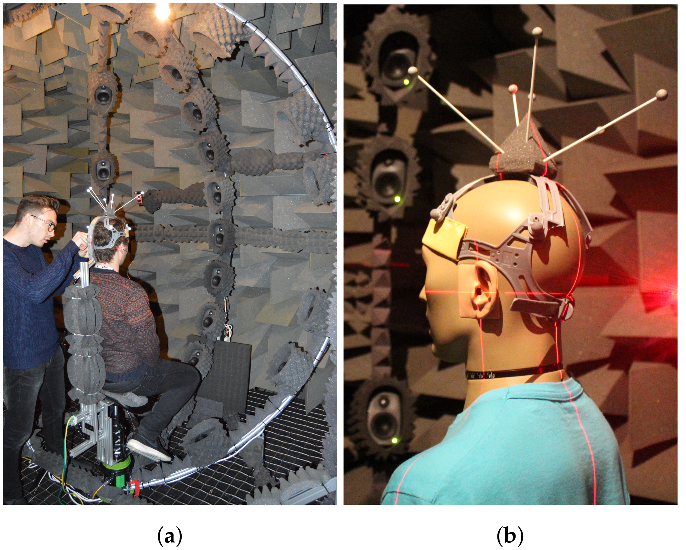
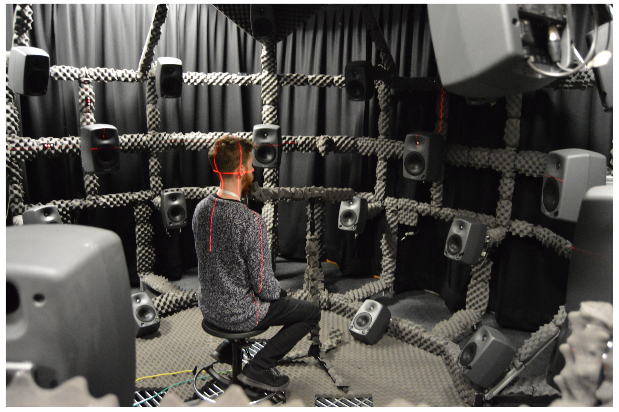
An acoustically treated HRTF measurement rig was designed for the anechoic chamber at the Audio Lab, University of York, York, UK (see Figure 2a [47]).
The set-up consisted of three static, vertical semi-circular arcs, each separated by 45° azimuth. Participants were sat centrally on a motor-controlled ‘saddle stool’, selected for its minimal acoustic occlusion. Their feet were tucked underneath their body, supported by a footrest. Their inter-aural axis was laser aligned to the precise centre of the loudspeaker array. Their head position was tracked in real time via a multi-purpose restraint, shown in Figure 2b. The restraint could be attached to a rigid back rest to help prevent unintentional head movement, as in Figure 2a. The restraint supported 10 reflective markers: six positioned asymmetricaly above the head and four positioned around the head. Four Optitrack Flex-3 Infra-Red motion capture cameras (www.optitrack.com/products/flex-3) tracked the 10 point rigid-body to within <0.1° via optical motion capture software, Motive (www.optitrack.com/products/motive) (Version 1.8.0 Final 64-bit). Utilizing this data, participants were rotated in place about the horizontal plane to a series of predetermined azimuthal positions by means of a Yaesu G-2800DXC motor and GS-232B serial interface (Yaesu. Cypress, CA, USA.).
Twenty-three Genelec 8010 loudspeakers (www.genelec.com/8010) were installed at 23 unique elevations at a radius of 1.2 m. In each case, the loudspeaker was aligned to its acoustic axis [48]. The 8010 was chosen for its small footprint and reliable frequency response (±2.5 dB) from 74–20 kHz.
Twelve elevations were measured at 15° intervals between −75° and 90°. These were necessary to measure the regular lattitude-longitude distribution [45]. Source localisation in the median plane is reported to be significantly worse than that in the horizontal plane [3]. A localisation blur of ±9° is reported for continuous familiar speech [49] whilst ±17° is reported for continuous unfamiliar speech [50]. Measurement intervals of 15° were considered to be of fine enough resolution to give an accurate representation of perceptual localisation cues without oversampling the subject unnecessarily.
A further 10 elevations were determined according to the common elevations coordinates of 11 typical Ambisonic loudspeaker layouts. An additional three layouts are composed of the same approximate elevations ±2°. A summary of these layouts and corresponding elevation coordinates is given in Table 3.
At a distance of 1.2 m, an error of 2° translates to a speaker displacement of 4.2 cm. This is small with respect to the size of the loudspeaker (18.1 cm) and main driver (12 cm). Considering such a minor displacement in relation to the resolution of the human ear, it is proposed that this error has little perceptual influence.
An elevation angle of −90° could not be measured as the area was blocked by the installation of the chair and motor. Instead, a nearest alternative angle of −81° was measured. In post-processing, these measurements were interpolated to approximate a measurement at −90°. For each ear, measurements were time aligned by their peak amplitude to the average delay of the subset. A linear interpolation was then performed in the time domain by calculating the average amplitude of each sample. Due to the nature of HRTF measurements made at such low elevations, the majority of high frequency detail is occluded by the legs/torso/chair. It is therefore reasonable to use an interpolated measurement, which will mainly preserve the low frequency cues.
As the subject was rotated, the relative azimuthal co-ordinate of each loudspeaker was redefined. A sequence of rotations was programmed such that these coordinates satisfied the intended configurations. At each azimuthal potion, the subject was stopped and a 2 s pause allowed any mechanical noise to settle. An overlapped exponential swept sine wave technique [51] was used to quickly and efficiently measure the IRs from all 23 loudspeakers, regardless of their direct affiliation to a configuration.
The use of a sinusoidal sweep is an effective technique to measure a source-receiver transfer function over a range of frequencies [52]. The recorded signal is convolved with an inverse (time-reverse and amplitude compensated) copy of the sweep to remove the time-smeared element of the input signal and re-align and normalize the various frequency components in the time domain. This is known as de-convolution and results in the IR of the source being located at the moment the input sweep finishes. To save time, the sweeps’ output from the loudspeakers may be overlapped provided that there is no interference between the IRs once the signals are deconvolved [51].
Twenty-four second sweeps separated by 0.15 s were performed with 0.1 s fade in/out half-Hanning windows over the frequency range 200–24 kHz. The entire process was automated with control software written in Max MSP (www.cycling74.com/products/max) and operated by technicians in an isolated control room via a dedicated Local Area Network.
Sixty-four stoppages were required for the measurement of the Ambisonic configurations. In addition, a regular set of measurements were required for the fixed lattitude-longitude distribution. A 1° resolution was chosen for the dummy subjects. This required a total of 399 stoppages. It generated 8802 unique measurements and took over 3 h to complete.
This was too long for a human to sit still, especially given the seat and head restraint. The horizontal resolution of the latitude-longitude configuration was therefore chosen on a subject by subject basis from two spatial distributions. In the first case, 11 subjects (seven admitted to database) were measured with 5° resolution. This required 127 stoppages, generated 2818 unique measurements and took approximately 1.25 h. In the second case, 18 subjects (11 admitted to database) were measured with 10° resolution. This required 95 stoppages, generated 2114 unique measurements and took approximately 1 h.
Recordings were made via a Fireface 400 interface (www.rme-audio.de/en/products/fireface_400.php) at 96 kHz sample rate and 24 bit resolution. Raw measurements were deconvolved using an unwindowed inverse sweep and the individual IRs were separated ensuring no overlap of the linear or harmonic distortion products of neighbouring sweeps in the deconvolution. IRs were trimmed to approximately 15 ms before and 10 ms after their peak amplitude to remove minor spurious reflections (assumed to come from the door frame of the anechoic chamber). An approximate signal-to-noise ratio of 65 dB was measured from the noise floor to the peak value of an IR measured from a frontal loudspeaker via a flat omnidirectional Gras 46AE measurement microphone (www.gras.dk/products/measurement-microphone-sets/product/140-46ae) positioned at the centre of the loudspeaker array.
3.2.2. Low Frequency Compensation
Due to the size of the loudspeakers’ diaphragms and the low-frequency limit of the anechoic chamber, frequencies below 200 Hz could not be reliably measured and were modelled instead. It is well established that the effects of a listener’s ear and pinnae are only influential at mid to high frequencies (>4000 Hz) [53]. At low frequencies (<400 Hz), analytical simulations such as those in [44] show that even a listener’s head barely effects (<1 dB) the frequency content of a signal either. It is therefore reasonable to adopt a low frequency model, similar to that in [54], which extends a flat frequency response and linear phase response below approximately 400 Hz.
Low frequency compensation was performed independently for each channel of each HRTF. A crossover frequency of 275 Hz was chosen. This balanced the preservation of natural higher-frequency content with the need to accommodate the crossover filter’s low frequency roll off when applied to the HRTF signals which only included data down to 200 Hz.
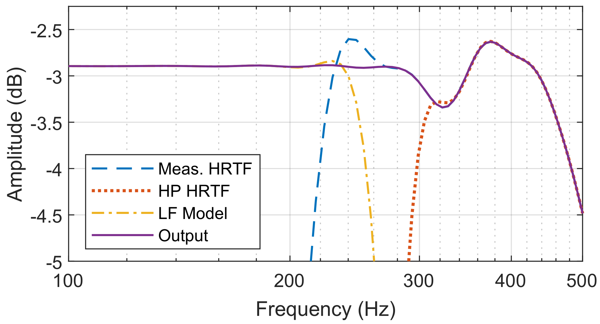
A Dirac pulse was generated with an amplitude and delay equal to the average amplitude and group delay of the signal to be extended between 250–300 Hz. This would typically position the Dirac after the peak of a HRTF. A phase response calculation was made at the crossover frequency and the Dirac shifted forward in time until the signals’ phases aligned precisely at 275 Hz. A forward shift ensured that the low frequency model remained well within any future amplitude windows applied to the HRTF around its peak. A pair of 4096 tap Finite Impulse Response (FIR) low/high pass filters were utilized to crossover the low-frequency model with the valid portion of the input signal. High order filters ensured that neighbouring frequencies were sufficiently attenuated to avoid de-constructive interference caused by slight phase misalignments in these regions. An example of the crossover between a measured HRTF and a corresponding low frequency model is shown in Figure 3.
A smooth transition between the High-Pass filtered HRTF and Low-Pass filtered low frequency model is shown in the output signal. Note the small amplitude variation (<1 dB) below 400 Hz in the measured signal.
3.2.3. Equalisation and Windowing
Correctly processed HRTFs require either diffuse-field or free-field equalisation. Both measures give a directionally independent common transfer function. Whilst diffuse field equalisation attempts to remove all commonality between a set of measurements, free field equalisation removes only the direct impact of the measurement system.
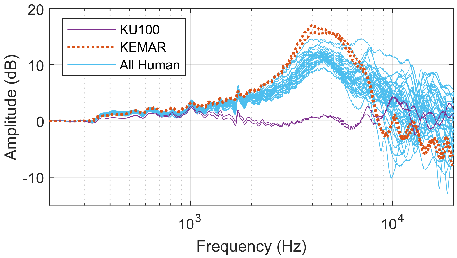
This is demonstrated in Figure 4, where the diffuse field response of each ear of each subject is shown after free field equalisation of both the average loudspeaker and respective binaural microphone responses. For the free-field equalisation, loudspeaker responses were measured using a flat response GRAS 46AE measurement microphone (www.gras.dk/products/measurement-microphone-sets/product/140-46ae) placed at the centre of the loudspeaker array. Microphone responses were calculated as follows: a 20–24 KHz sine sweep was output from a Genelec 8040 loudspeaker (www.genelec.com/support-technology/previous-models/8040a-studio-monitor) in the anechoic chamber. The sweep was simultaneously recorded by a flat-response GRAS 46AE measurement microphone and each of the individual binaural microphones one at a time. In every case, the binaural microphone was placed as close as possible to the measurement microphone. A Fast Fourier Transform (FFT) was taken of each recording and the spectral response of the measurement microphone was subtracted from that of each binaural microphone. This resulted in the spectral responses of each binaural microphone. Inverse linear-phase FIR filters were computed using Kirkeby and Nelson regularization [55], which could be applied by means of convolution.
Despite the free-field equalisation, the diffuse field responses of the KEMAR mannequin and human subjects all follow a similar trend, peaking at around 4 kHz. The KEMAR response peaks highest at about 17 dB. It is suspected that this peak is a result of ear canal resonance. This would explain both the similarity and slight variation between subjects as the microphones could not always be placed at exactly the same depth within each participant’s ears. It would also explain the amplitude of the KEMAR response whose microphones are housed internally further within the ear canal mould. In contrast, the response of the KU100 is relatively flat. This is to be expected as the dummy head is pre-calibrated with a diffuse field equalisation filter [56].
Consequently, within the SADIE II database, all measurements are diffuse field equalised. This choice was made for a number of reasons:
- a large enough set of data points was being captured to make diffuse field equalisation viable;
- it would take into account the free field response on the system in situ i.e., influences due to the placement of the microphone capsule within the ear canal;
- it would compensate for any generic response of the post-processing (e.g., windowing);
- it would equate the average frequency response of each dataset to provide a timbral consistency across the database (recall the KU100 is pre-calibrated with a diffuse field equalisation filter [56]);
- it helps to ensure the reproduction of accurate tone colour considering the random directions from which many reverberant reflections could emanate from [3].
The equalisation was performed in two stages: before and after a windowing operation imposed to reduce the tap length of the filters. For each stage, the power average response of the dataset was calculated in the frequency domain for each ear of each subject. A weighting was applied to the contribution of each measurement based on a solid angle calculation of neighbouring measurements. This ensured that clustered measurements did not over-represent a particular direction in the average. Inverse linear-phase FIR filters were calculated from the diffuse field response using Kirkeby and Nelson regularization [55] to perform each equalisation.
Stage one was designed to compensate for the response of the measurement system. Input data was left unwindowed to preserve as much of the original signal content as possible. In addition, 1/3rd octave band smoothing was used to prevent overly-sharp peaks or notches appearing in the frequency response of the inverse filter and exacerbating the time-domain aliasing.
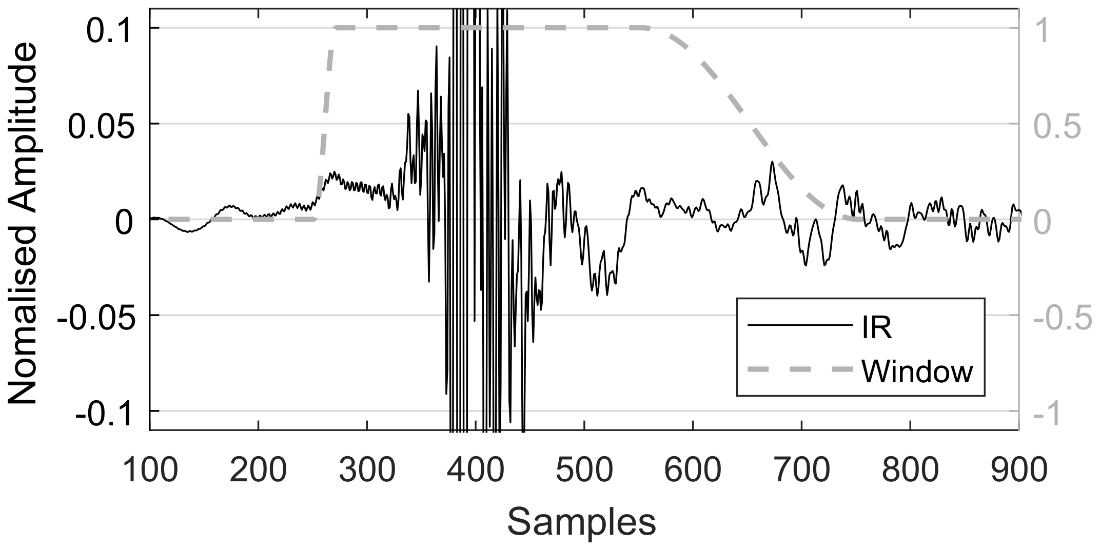
IRs were then windowed to 500 samples (approximately their final length) by means of a 20 sample half Hanning window and 130 sample pad before each peak and a 150 sample pad and 200 sample half Hanning window after (see Figure 5).
The proportions and relative position of this window affected both the preservation of the filter’s frequency response and the final diffuse field response of the dataset. By biasing the length of the fade out over the post-peak pad and shifting the window to preserve more of the pre-peak signal, the diffuse field variance can be reduced. However, accurate preservation of the frequency response generally required as much of the post-peak signal to remain as intact as possible.
Systematic frequency domain errors introduced by the windowing operation were compensated for by a second stage of diffuse field equalisation. This equalisation was performed on the windowed IRs with 1/5th octave band smoothing. As the first stage of equalisation had already considerably smoothed out the diffuse field response, a less smooth filter was required.
The IRs were time aligned and trimmed to 512 samples (256 samples at 48/44.1 KHz) inclusive of 10 sample fade in/out half Hanning windows. It was ensured that at least 180 samples remained before each peak and at least 230 samples remained after. This left approximately 100 samples to account for the variances in peak onset time due to ITDs.
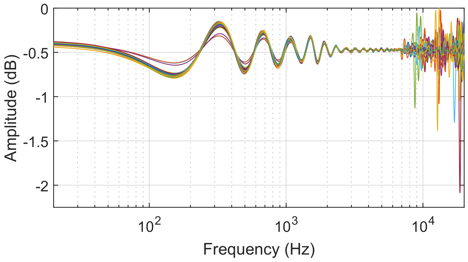
Figure 6 shows the final normalised diffuse field response of each ear of each subject calculated after all post-processing: deconvolution and separation of original recordings, low frequency compensation, stage 1 diffuse field equalisation, windowing, stage 2 diffuse field equalisation, and trim to 512 samples.
Comparing the magnitudes of the frequency bins of each response, 95% fall within a 0.33 dB range (approximately −0.35 dB and −0.65 dB). The pattern followed by each response below approximately 7 KHz can be attributed to the windowing parameters.
3.3. Binaural Room Impulse Responses
Although not relevant to this particular study, there is a lack of comparative HRTF/BRIR measurements taken of the same subjects within the same time frame utilizing the same post-processing procedures. We therefore include details of such measurements in the hope that they may be of use in future work.
Participants were led directly from the anechoic chamber to a treated listening room where BRIRs were measured from an acoustically calibrated 50 point Lebedev grid loudspeaker array (see Figure 7).
Measurements of this configuration are particularly useful as nested within it are the 6- and 26-point Lebedev grids [59]. This particular array utilizes two types of loudspeaker. In addition, 40 Genelec 8030 s are supported by 10 Genelec 8040 s, for low frequency reconstruction. The rig is enclosed by a thick curtain. Measurements of the KU100 and KEMAR mannequins demonstrate reverberation times of around 50–65 ms for a drop of 60 dB, dependent on speaker location.
Participants were sat on a stool and their interaural axis was laser aligned to the centre of the array. A rigid, acoustically dampened chin rest was used to ensure the participant kept their head still throughout the measurement procedure. Three-second exponential swept sine waves were played out of each loudspeaker one at a time over the range 20–24 kHz. Recordings were made via a MOTU UltraLite-Mk3 Hybrid audio interface (www.motu.com/products/motuaudio/ultralite-mk3) at a 96 kHz sample rate and 24 bit resolution.
After deconvolution, free field equalisation of each of the microphone’s frequency responses was performed using linear-phase FIR filters. Microphone responses were calculated as discussed in Section 3.2.3. By only equalising for the microphone responses (not loudspeakers), it ensured that the measurements most accurately represented the real-world listening conditions of the loudspeaker array. The BRIRs were trimmed to 0.3 s inclusive of 10 sample fade in/out half Hanning windows.
3.4. Headphone Equalization
Headphone Impulse Responses (HpIRs) are IR measurements taken from the left and right transducers of a pair of headphones. Measurements of this type do not include any interaural crosstalk (i.e., the response of the left transducer in the right ear). Headphone Equalisation (HpEQ) may be performed by implementing a filter with the inverse response of a HpIR. This compensates for the transfer function of a pair of headphones coupled to a person’s outer ear and is crucial for ensuring the accurate reception of binaural signals [60,61].
Without removing the binaural microphones, participants were asked to put on a pair of open-back Beyerdynamic DT990 Pro headphones (europe.beyerdynamic.com/dt-990-pro.html). A 3 s exponential swept sine wave was output from each transducer (one at a time) and recorded through the MOTU interface. This was repeated 10 times. In between each pair of measurements, the participant was asked to remove the headphones completely and place them back on their head.
After deconvolution, the IRs for each ear were power averaged together in the frequency domain. An inverse FFT followed by a circular shift of half the FFT size brought the data back into a stable format in the time domain (i.e., a continuous central peak). The binaural microphone frequency responses were equalised out of the signals. The HpIRs were trimmed to 2048 samples and a full length Hanning window was applied.
Linear Phase HpEQ filters were generated by inverting the frequency responses of the HpIR filters. This was done over the range 120–24 kHz with 1/5th octave band smoothing. Responses were trimmed to 2048 samples and amplitude weighted by a full length Hanning window.
4. Listening Test: HRTF Preference
A listening test was conducted to investigate the existence of quantifiable timbral and/or spatial attributes within individual and non-individual HRTF measurements. Sixteen participants (13 male, 1 female, 2 non-binary, ages: 20–63 (majority 20–30)) all of whom were admitted to the SADIE II database were re-recruited for the test. All subjects gave their informed consent for inclusion before they participated in the study. The protocol was approved by the University of York Physical Sciences Ethics Committee. Participants were presented with a set of auditory stimuli over headphones and were asked to rate each one based on four attributes as defined in Section 2: brightness, richness, externalisation and preference.
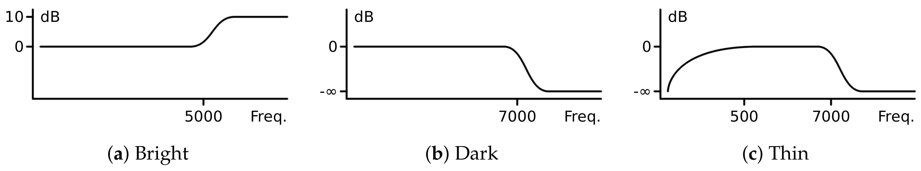
The terms brightness and richness were described to each participant along with example audio files containing filtered exerts of music. Three examples were filtered according to frequency response plots shown in Figure 8.
A high boost simulated a bright signal, a high cut simulated a dark signal and a low and high cut simulated a thin signal. One further example was left unfiltered to simulate a rich signal.
The term externalisation is not so easy to conceptualise. To verify the effectiveness of any example file would have required the verification of the spatial filters used to create such a file. This was in part the purpose of this study. Participants were instead provided with a graphical depiction of the soundfield and were advised that effective externalisation would be as if they were hearing the sources in real life. Preference required not only a sense on externalisation, but also a pleasant timbre and overall feeling of realism. Participants were given the opportunity to ask any questions relating to the definitions of each term.
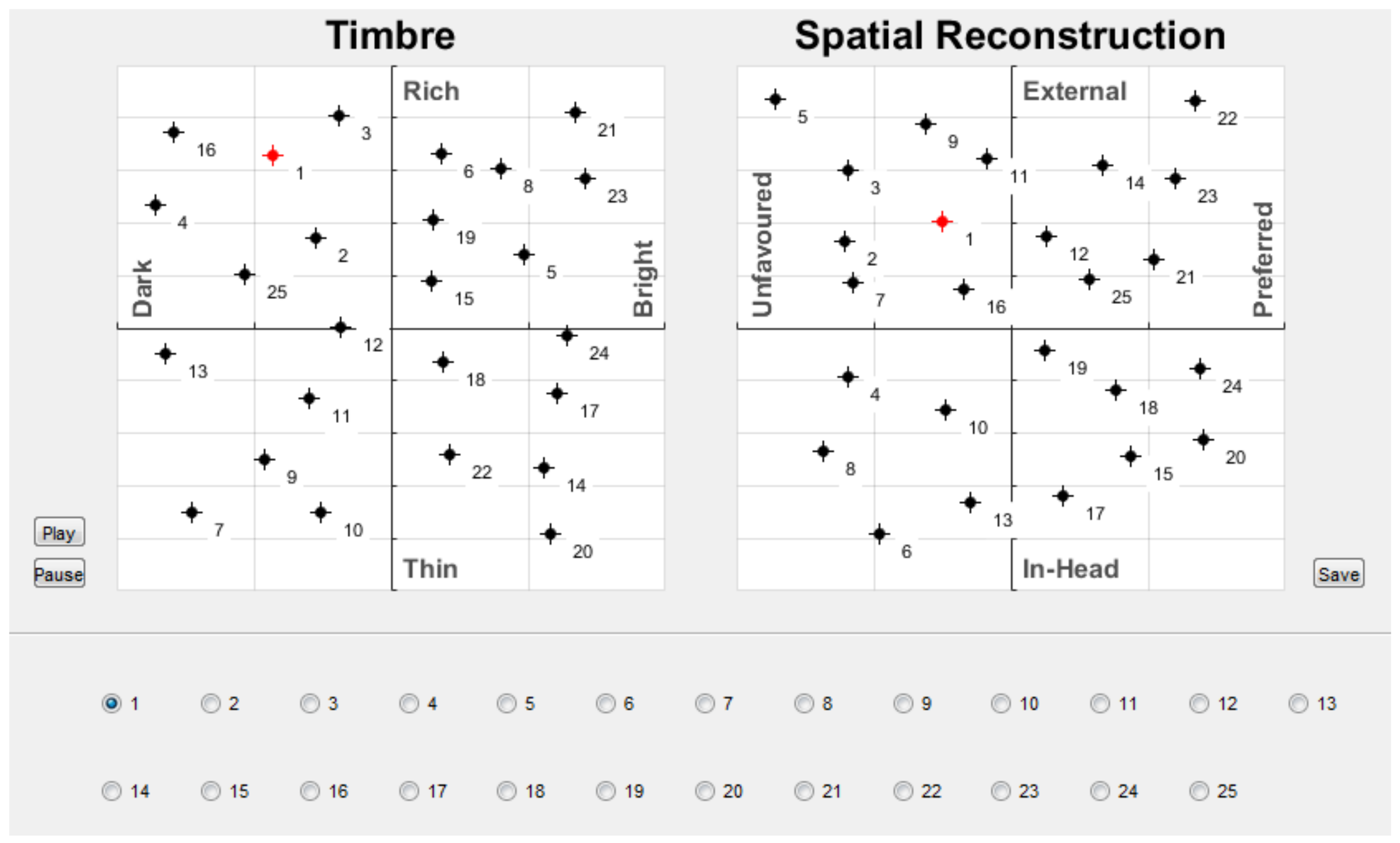
During the test, participants were able to freely switch between the set of stimuli over a continuous looped playback. Ratings were performed using the graphical interface shown in Figure 9.
Participants were required to drag a marker corresponding to a stimuli to a point on a graph. Two graphs were used to represent the four attributes on continuous scales. Brightness and richness were represented by the x- and y-axes of one graph and preference and externalisation the axes of the other. The interface allowed participants to easily compare and adjust the ratings they were giving to each stimuli. They were instructed to make use of the entire range.
Noise bursts and other broadband signals are common stimuli used throughout listening tests; however, such unfamiliar and unnatural audio is inappropriate for this type of study. A common alternative is to use speech [13,15,62]. Whilst this is a more ecological than noise, it is relatively band limited and lacks low frequencies especially. The stimuli used should represent examples of everyday bianural audio and as such should elicit the same or at least similar perceptual characteristics [36]. For example, whilst it would be quite unusual to discuss the brightness of radio static, a similar discussion about the sound of a piano would be relatively common.
With this in mind, approximately a minute and a half of music was composed in a jazz style using a range of non-reverberant VST MIDI samplers. These included a stereo drum set, stereo piano, flute, trumpet, trombone and double bass for a well balanced mix covering a large range of frequencies. The ensemble was binaurally spatialised by convolving individual audio stems with HRTFs spaced at 45° increments around the horizontal plane, starting at 0°, and summing the results. Stereo sources were convolved with adjacent HRTFs to mimic phantom source phenomena in real world listening [63]. 20 binaural signals were produced using each of the Twenty HRTF measurement sets admitted to the SADIE II binaural database, discussed in Section 3.1.
In addition, five anchor stimuli were presented: four stereo mixes and one mono mix. The stereo mixes were rendered by amplitude weighting the audio stems based on a constant power panning law. The mono mix was rendered by the equal summation of all sources. Of the four stereo mixes, three were degraded by the same filters as the example stimuli and as depicted in Figure 8. One stereo mix was left unfiltered to simulate a rich signal. The mono mix simulated a non-spatial signal.
All 25 stimuli, normalised to an RMS level, were presented to each participant in a random order over Beyerdynamic DT-990 Pro open-back headphones (europe.beyerdynamic.com/dt-990-pro.html) via a Fireface UCX interface (www.rme-audio.de/en/products/fireface_ucx.php). Participants were asked to adjust the volume of playback to a comfortable listening level i.e., a level at which they would normally listen. Personalised headphone equalisation was used in each case. Equalization filters previously measured as part of the SADIE II database, presented in Section 3.4, were used. The same pair of headphones were used for this test as were measured for the database.
5. Results
Each subject’s ratings were normalized with respect to mean value (0) and standard deviation as recommended by ITU-R BS.1284-1 [25]. The combined ratings for each attribute were then normalized to a maximum absolute value of ±1. The responses to each stimuli are presented as box plots in Figure 10 in order of mean preference.
Stimuli are identified by either the anchor they represent, or by the subject whose HRTFs were used to render the signals. To preserve anonymity, human subjects are referred to as H[3–20]. Included on the plots are the ratings given to each stimuli by the owner of the respective HRTFs. This is referred to as the Personal Rating.
The average values and narrow ranges of the thin, dark and bright anchors (stereo tracks) validate the participants understanding of the attributes. The results of the mono anchor are surprisingly optimistic. Despite averaging amongst the lowest scores in both externalisation and preference, the confidence intervals and error bars extend to well within the ranges of higher scoring HRTF sets. This indicates the significance of timbre in rendering systems.
The responses to each stimuli were tested for normality with a Lilliefors test which failed to reject the null-hypothesis of normality at the 5% significance level. The significance of the ratings given to each stimuli for each attribute were explored by one-way repeated measure ANOVA with post hoc analysis. Violations of the assumption of sphericity were identified by Mauchly’s tests and Greenhouse–Geiser corrections were applied in the calculations of p-values. Results are presented in Table 4.
A p-value of below 5% indicates that we may say with 95% confidence that the average results do truly vary. Greatest significance is seen with respect to preference, followed by timbral attributes: brightness and richness. A significant difference is not seen with respect to externalisation. Together with Figure 10, these results reinforce that timbre must play a considerable role in HRTF selection.
A post hoc pairwise comparison of the mean ratings given to each stimuli was undertaken using Tukey’s Honestly Significant Difference test procedure. This revealed seven significant differences between stimuli with respect to preference, two with respect to richness and five with respect to brightness. Zero significant results were seen with respect to externalisation. A summary is given in Table 5.
By virtue of the fact that diffuse field equalised HRTFs were used throughout the test, these differences in timbral and spatial features must be attributed to the individual spectral notches of the HRTFs and not to any general frequency response of the individual.
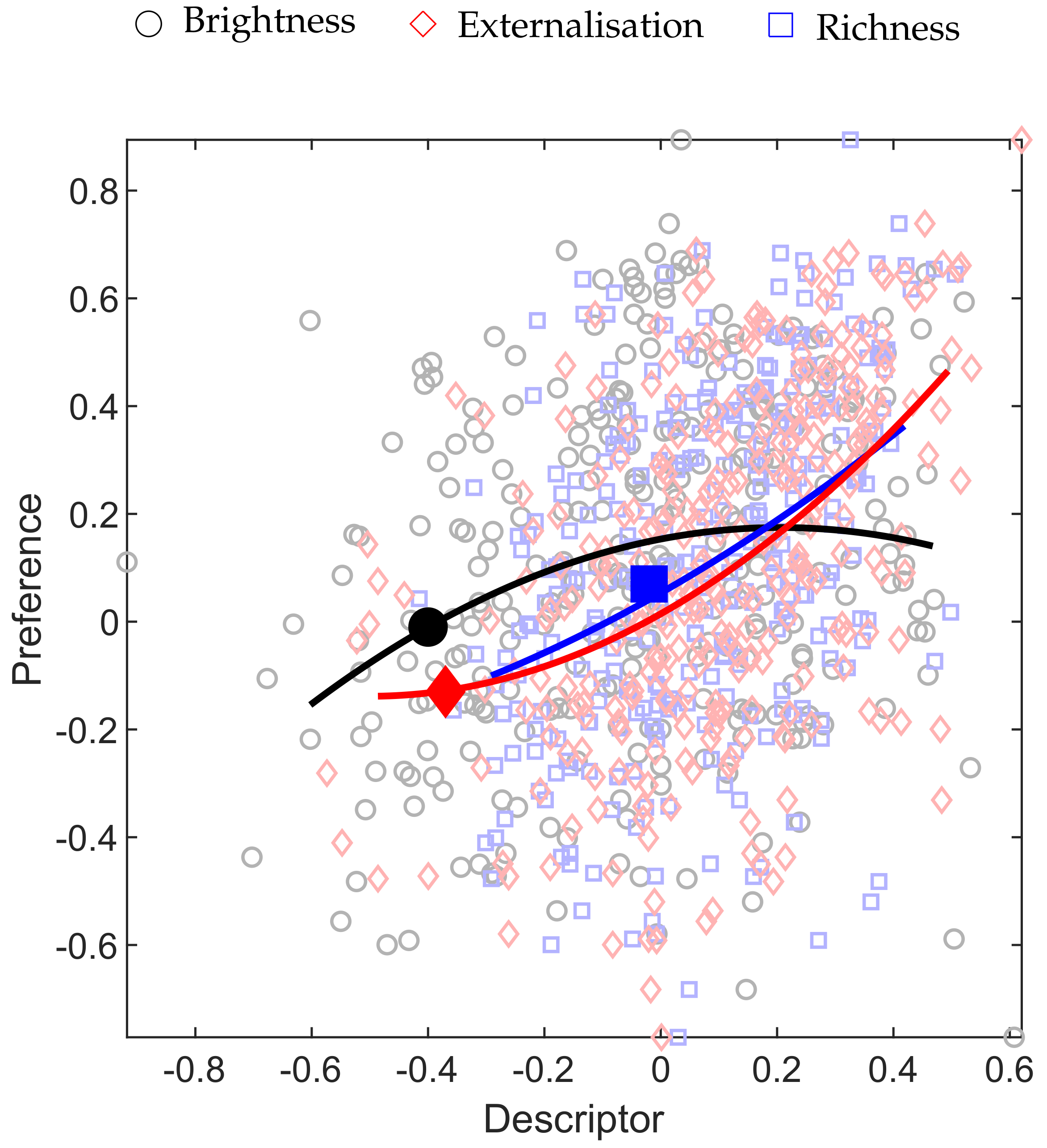
The correlation of brightness, richness and externalisation with respect to preference is plotted in Figure 11. The graph directly compares the attribute ratings given by each participant to each stimuli. Anchors and anomalies identified in Figure 10 are excluded from this plot. Second order polynomial lines of best fit indicate a positive correlation between richness, externalisation and preference. A slight preference for neutral brightness can be seen.
Analyzing the correlation of such a mapping of brightness to preference is challenging due to its non-linearity. We therefore define a new parameter brightness* that is the deviation of the brightness rating from an optimal value of 0.2 (read from Figure 11).
By doing this, we may consider the correlation of brightness* such that a higher rating is indicative of preference. A summary of the Pearson’s correlation coefficient values for each pair of attributes is given in Table 6.
6. Discussion
From these results, we present three key findings. The first is that there are significant differences in the attribute ratings given to particular HRTF sets by a general audience. The second is that there exists some correlation between these attributes, for example that of externalisation, richness and preference, but that this correlation is not high. The third is that individual measurements were not perceived by subjects to be of optimal performance.
Overall, it is the HRTFs of the dummy mannequins that are most preferred. Surprisingly, it is the HRTFs of the head without shoulders (the KU100) that received the highest rating for preference. This is despite averaging similar or less favourable ratings than the measurements of KEMAR, H11, H20 and H7 with respect to all other attributes, according to general correlations shown in Figure 11. It is likely, therefore, that there exist other factors not identified in this study that have a stronger influence on overall preference.
There are two major differences between the measurements of the dummy heads and the human participants: movement and microphones. Despite best efforts, some movement is inevitable with human subjects, the binaural heads on the other hand remain perfectly still. Larger in-built microphones were also utilised for the dummy heads. Significant differences between the preference ratings of human measurements (H20, H7, H9) and (H19), however, indicate that microphone selection alone cannot be the sole cause of preference. It is therefore proposed that the stillness with which a participant sits could impact the quality of measurement and hence the performance of the HRTFs.
We see strongest relevant correlation between the attributes externalisation and preference with a Pearson’s correlation coefficient value of 0.46. However, we note that this does not indicate a particularly strong correlation. A similar result is seen between richness and preference whilst brightness* appears to correlate relatively poorly with all other attributes. A slight preference for brighter timbres over darker timbres may be interpreted from Figure 11. This is confirmed by the positive correlation coefficient (, see Table 6) calculated between brightness and preference.
These values indicate a slight correlation between the attributes tested in this study. However, it is in fact of more interest to note the lack of strong correlation. Such results show that HRTFs may be rated as highly preferable regardless of their timbral or spatial characteristics. Therefore, selection of an optimal HRTF remains a complex task and likely depends on the application.
A key result is the randomness with which a participant rated their own measurements. Andreopoulou [20] comments on the repeatability and hence reliability (or lack thereof) of HRTF ratings. They conclude that although, in general, HRTF rating is a difficult task, repeatability of results is significantly higher at the extreme ends of the response scales. This indicates that had individual measurements significantly out-performed non-individual measurements, as one might expect, we should have seen consistent results. However, this was not the case.
We find that individual measurements may not necessarily be the optimal tool for binaural rendering, especially when considering the more general requirements of good spatial audio reproduction beyond localisation. Such claims are echoed throughout the literature [7,8]. In our case, only one participant (H9) rated their individual measurements as sounding the most external. No participants rated their individual measurements as the most preferred and 81% of participants preferred the KU100 HRTFs to their own. Despite almost certainly improving source localisation in binaural reproduction [12,13,14], this finding calls into question the usefulness of individual HRTF measurements when one considers a more open quality of experience evaluation.
These findings have direct implications within the design on spatial audio rendering systems. The purpose of the system must be identified before an HRTF set is selected for spatial reproduction. For example, in gaming environments, it is understandable that accurate source localisation may be prioritized. However, within the audio and film industries, one may argue that it is the quality of sound that must be preserved. As such, designers may utilize individual measurements for games, but opt for more generally preferred HRTF sets (for example, that of the KU100) for entertainment.
It is important to consider that timbral and spatial preferences will vary between listener and that this will have contributed to the spread of results in this study. However, such problems have existed within non-spatial audio applications for decades and as such we must consider a generally accepted average. It is unlikely that a single HRTF set will ever be able to perform optimally for every person across every imaginable attribute. However, this study finds that a single HRTF set may be able to perform highly within key attributes for a wide range of subjects.
7. Conclusions
This paper has presented a perceptual listening test in which participants were asked to evaluate both individual and non-individual binaural renderings of a jazz ensemble on four scales: brightness, richness, externalisation and preference. Results show significant differences in the ratings given to particular HRTF sets at the 95% confidence interval. An overall preference for the measurement set of the KU100 dummy head is seen, followed closely by the the measurement set of the KEMAR mannequin. A slight preference is shown for rich and external stimuli of a neutral/slightly bright timbre. Very little correlation is seen with respect to the responses given to stimuli generated with individual HRTFs.
Details of the measurement and post processing of the SADIE II Database were also presented. Diffuse field equalised HRTFs, BRIRs and HpIRs data of 20 subjects (2 dummy, 18 human) are now available online for use in similar tests. The database represents the largest measured HRTF datasets for both human subjects and the KEMAR mannequin currently available. Furthermore, it is the only database which provides comparative echoic and anechoic measurements.
The results of this paper lead to questions regarding the future of HRTF measurement and binaural rendering. Source localisation, shown to improve with individual measurements, must be carefully balanced against timbral and spatial qualities of competing measurement sets. For now, this paper serves to promote the significance of non-localisation based HRTF attributes and the compelling performance of the KU100 measurement set.
Author Contributions
Conceptualization, C.A. and G.K.; Data Curation, C.A. and L.T.; Formal Analysis, C.A.; Funding Acquisition, G.K.; Investigation, C.A.; Methodology, C.A. and G.K.; Project Administration, C.A.; Software, C.A. and G.K.; Supervision, D.M. and G.K.; Validation, C.A.; Visualization, C.A.; Writing—Original Draft, C.A.; Writing—Review and Editing, C.A., D.M. and G.K.
Funding
This research is supported by a Huawei Innovation Research Partnership. The research was funded by the Engineering and Physical Sciences Research Council (EP/M001210/1).
Acknowledgments
The authors would like to thank Andrew Chadwick for his technical assistance in the construction of the measurement rig. They would also like to thank the measurement and listening test volunteers for their valuable time.
Conflicts of Interest
The authors declare no conflict of interest. The founding sponsors had no role in the design of the study; in the collection, analyses, or interpretation of data; in the writing of the manuscript, and in the decision to publish the results.
References
- Riaz, H.; Stiles, M.; Armstrong, C.; Lee, H.; Kearney, G. Multichannel Microphone Array Recording for Popular Music Production in Virtual Reality. In Proceedings of the 143rd Convention Audio Engineering Society (AES), New York, NY, USA, 18–21 October 2017; pp. 1–5. [Google Scholar]
- Hong, J.; He, J.; Lam, B.; Gupta, R.; Gan, W.S. Spatial Audio for Soundscape Design: Recording and Reproduction. Appl. Sci. 2017, 7, 627. [Google Scholar] [CrossRef]
- Blauert, J. Spatial Hearing: The Phychophysics of Human Sound Localization; MIT Press: Cambridge, MA, USA, 1997. [Google Scholar]
- Møller, H.; Sorensen, M.F.; Hammershoi, D.; Jensen, C.B. Head-Related Transfer-Functions of Human-Subjects. J. Audio Eng. Soc. 1995, 43, 300–321. [Google Scholar]
- Menzer, F.; Faller, C.; Lissek, H. Obtaining binaural room impulse responses from b-format impulse responses using frequency-dependent coherence matching. IEEE Trans. Audio Speech Lang. Process. 2011, 19, 396–405. [Google Scholar] [CrossRef]
- Vorländer, M. Auralization: Fundamentals of Acoustics, Modelling, Simulation, Algorithms and Acoustic Virtual Reality, 1st ed.; Springer: Berlin, Germany, 2008. [Google Scholar]
- Nicol, R.; Gros, L.; Colomes, C.; Warusfel, O.; Noisternig, M.; Bahu, H.; Katz, B.F.G.; Simon, L.S.R. A Roadmap for Assessing the Quality of Experience of 3D Audio Binaural Rendering. In Proceedings of the EAA Joint Symposium on Auralization and Ambisonics, Berlin, Germany, 3–5 April 2014; pp. 100–106. [Google Scholar]
- Usher, J.; Martens, W.L. Perceived Naturalness Of Speech Sounds Presented Using Personalized Versus Non-personalized HRTFs. In Proceedings of the International Conference on Auditory Display, Montréal, QC, Canada, 26–29 June 2007; pp. 10–16. [Google Scholar]
- Wightman, F.L.; Kistler, D.J. Headphone simulation of free field listening I: Stimulus synthesis. J. Acoust. Soc. Am. 1989, 85, 858–867. [Google Scholar] [CrossRef] [PubMed]
- Wightman, F.L.; Kistler, D.J. Headphone simulation of free-field listening. II: Psychophysical validation. J. Acoust. Soc. Am. 1989, 85, 868–878. [Google Scholar] [CrossRef] [PubMed]
- Hur, Y.; Lee, S.P.; Park, Y.; Youn, D. Efficient individualization of HRTF using critical-band based spectral cues control. J. Audio Eng. Soc. 2008, 180, 167–180. [Google Scholar] [CrossRef]
- Seeber, B.U.; Fastl, H. Subjective selection of non-individual head-related transfer functions. In Proceedings of the International Conference on Auditory Display, Boston, MA, USA, 6–9 July 2003. [Google Scholar]
- Møller, H.; Sørensen, M.F. Binaural technique: Do we need individual recordings? J. Audio Eng. Soc. 1996, 44, 451–469. [Google Scholar]
- Wenzel, E.M.; Arruda, M.; Kistler, D.J.; Wightman, F.L. Localization using nonindividualized head-related transfer functions. J. Acoust. Soc. Am. 1993, 94, 111–123. [Google Scholar] [CrossRef] [PubMed]
- Begault, D.R.; Wenzel, E.M.; Anderson, M.R. Direct comparison of the impact of head tracking, reverberation, and individualized head-related transfer functions on the spatial perception of a virtual speech source. J. Audio Eng. Soc. 2001, 49, 904–916. [Google Scholar] [CrossRef] [PubMed]
- Pike, C.; Melchoir, F. An Assessment of Virtual Surround Sound Systems for Headphone Listening of 5.1 Multichannel Audio; Technical Report; BBC: Salford, NY, USA, 2013. [Google Scholar]
- Pike, C.; Melchior, F.; Tew, A.I. Descriptive analysis of binaural rendering with virtual loudspeakers using a rate-all-that-apply approach. In Proceedings of the AES Conference on Headphone Technology, Aalborg, Denmark, 24–26 August 2016. [Google Scholar]
- Kearney, G.; Doyle, T. A HRTF Database for Virtual Loudspeaker Rendering. In Proceedings of the Audio Engineering Society, Victoria, Australia, 7–10 May 2015. [Google Scholar]
- Katz, B.F.G.; Parseihian, G. Perceptually based head-related transfer function database optimization. J. Acoust. Soc. Am. 2012, 131, EL99–EL105. [Google Scholar] [CrossRef] [PubMed]
- Andreopoulou, A.; Katz, B.F.G. Investigation on Subjective HRTF Rating Repeatability. Audio Eng. Soc. Conv. 2016, 140, 9597:1–9597:10. [Google Scholar]
- Schönstein, D.; Katz, B.F.G. Variability in Perceptual Evaluation of HRTFs. J. Audio Eng. Soc. 2012, 60, 783–793. [Google Scholar]
- Andreopoulou, A.; Katz, B.F.G. On the Use of Subjective Hrtf Evaluations for Creating Global Perceptual Similarity Metrics of Assessors and Assessees. In Proceedings of the 21st International Conference on Auditory Display (ICAD 2015), Graz, Austria, 8–10 July 2015; pp. 13–20. [Google Scholar]
- Andreopoulou, A.; Katz, B.F.G. Subjective HRTF evaluations for obtaining global similarity metrics of assessors and assessees. J. Multimodal User Interfaces 2016, 10, 259–271. [Google Scholar] [CrossRef]
- Huopaniemi, J.; Zacharov, N.; Karjalainen, M. Objective and Subjective Evaluationof Head, Related Transfer Function Filter Design. J. Audio Eng. Soc. 1999, 47, 218–239. [Google Scholar]
- ITU (International Telecommunication Union). BS.1284-1 General Methods for the Subjective Assessment of Sound Quality; Technical Report; ITU: Geneva, Switzerland, 2003. [Google Scholar]
- EBU Tech 3286-E. Assessment Methods for the Subjective Evaluation of the Quality Of Sound Programme Material—Music. 1997. Available online: https://tech.ebu.ch/docs/tech/tech3286.pdf (accessed on 19 October 2018).
- Lorho, G.; Huopaniemi, J.; Zacharov, N.; Isherwood, D. Efficient HRTF synthesis using an interaural transfer function model. Eur. Signal Process. Conf. 2000, 2000, 80–83. [Google Scholar]
- Pulkki, V.; Karjalainen, M.; Huopaniemi, J. Analyzing virtual sound source attributes using a binaural auditory model. J. Audio Eng. Soc. 1999, 47, 203–217. [Google Scholar]
- ITU. BS.1387-1 Method for Objective Measurements of Perceived Audio Quality; Technical Report; International Telecommunication Union: Geneva, Switzerland, 2001. [Google Scholar]
- Thiede, T.; Treurniet, W.C.; Bitto, R.; Beerends, J.G.; Olomes, C.C.; Keyhl, C.H.; Member, A.E.S.; Feiten, A.N.D.B.; Memb, A.E.S.; Ptt, R.; et al. PEAQ—The ITU standard for objective measurement of perceived audio quality. J. Audio Eng. Soc. 2000, 48, 3–29. [Google Scholar]
- Berg, J.; Rumsey, F. Identification of Perceived Spatial Attributes of Recordings by Repertory Grid Technique and other methods. In Proceedings of the 106th AES Convention: Preprints, Audio Engineering Society, Munich, Germany, 8–11 May 1999. [Google Scholar]
- Koivuniemi, K.; Zacharov, N. Convention Paper 5424. In Proceedings of the 111st AES Convention: Audio Engineering Society (AES), New York, NY, USA, 30 November–3 December 2001. [Google Scholar]
- Lindau, A.; Erbes, V.; Lepa, S.; Maempel, H.J.; Brinkman, F.; Weinzierl, S. A spatial audio quality inventory (SAQI). Acta Acust. United Acust. 2014, 100, 984–994. [Google Scholar] [CrossRef]
- Lokki, T.; Pätynen, J.; Kuusinen, A.; Tervo, S. Disentangling preference ratings of concert hall acoustics using subjective sensory profiles. J. Acoust. Soc. Am. 2012, 132, 3148–3161. [Google Scholar] [CrossRef] [PubMed]
- Pearce, A.; Brookes, T.; Mason, R. Timbral attributes for sound effect library searching. In Proceedings of the 2017 AES International Conference on Semantic Audio, Erlangen, Germany, 22–24 June 2017. [Google Scholar]
- Simon, L.S.R.; Zacharov, N.; Katz, B.F.G. Perceptual attributes for the comparison of head-related transfer functions. J. Acoust. Soc. Am. 2016, 140, 3623–3632. [Google Scholar] [CrossRef] [PubMed]
- Gerzon, M.A. Practical Periphony: The Reproduction of Full-Sphere Sound. In Proceedings of the 65th AES Convention: Audio Engineering Society (AES), London, UK, 25–28 February 1980. [Google Scholar]
- Daniel, J. Représentation De Champs Acoustiques, Application à La Transmission Et à La Reproduction De Scènes Sonores Complexes Dans Un Contexte Multimédia. Ph.D. Thesis, l’Université Paris, Paris, France, 2001. [Google Scholar]
- ARI HRTF Database. Available online: https://www.kfs.oeaw.ac.at/index.php?view=article&id=608&lang=en (accessed on 19 October 2018).
- Algazi, V.; Duda, R.; Thompson, D.; Avendano, C. The CIPIC HRTF database. In Proceedings of the 2001 IEEE Workshop on the Applications of Signal Processing to Audio and Acoustics, New York, NY, USA, 21–24 October 2001. [Google Scholar]
- LISTEN HRTF DATABASE. Available online: http://recherche.ircam.fr/equipes/salles/listen/ (accessed on 19 October 2018).
- Gupta, N.; Barreto, A.; Joshi, M.; Agudelo, J.C. HRTF database at FIU DSP Lab. In Proceedings of the 2010 IEEE International Conference on Acoustics Speech and Signal Processing (ICASSP), Dallas, TX, USA, 15–19 March 2010; pp. 169–172. [Google Scholar]
- Gardner, W.G.; Martin, K.D. HRTF measurements of a KEMAR. J. Acoust. Soc. Am. 1995, 97, 3907–3908. [Google Scholar] [CrossRef]
- Bernschütz, B. A Spherical Far Field HRIR/HRTF Compilation of the Neumann KU 100. In Proceedings of the 40th Italian (AIA) Annual Conference on Acoustics and the 39th German Annual Conference on Acoustics (DAGA) Conference on Acoustics, Merano, Italy, 8–21 March 2013; p. 29. [Google Scholar]
- Description of Gaussian, Fixed, Fixed Offset, Regular, Curvilinear Grids. 2018. Available online: https://www.ncl.ucar.edu/Document/Functions/sphpk_grids.shtml (accessed on 19 October 2018).
- Lecomte, P.; Gauthier, P.A.; Langrenne, C.; Berry, A.; Garcia, A. A fifty-node lebedev grid and its applications to ambisonics. J. Audio Eng. Soc. 2016, 64, 868–881. [Google Scholar] [CrossRef]
- Armstrong, C.; Chadwick, A.; Thresh, L.; Damian, M.; Kearney, G. Simultaneous HRTF Measurement of Multiple Source Configurations Utilizing Semi-Permanent Structural Mounts. In Proceedings of the AES 143rd Convention, New York, NY, USA, 18–21 October 2017. [Google Scholar]
- 8010A Operating Manual. Technical Report. Available online: https://www.genelec.com/sites/default/files/media/Studio%20monitors/8000%20Series%20Studio%20Monitors/8010A/8010a_opman.pdf (accessed on 19 October 2018).
- Damaske, P.; Wagener, B. Richtungshorversuche fiber einen nachgebildeten Kopf. Acta Acust. United Acust. 1969, 21, 30–35. [Google Scholar]
- Blauert, J. Ein Versuch zum Richtungshören bei gleichzeitiger optischer Stimulation. Acta Acust. United Acust. 1970, 23, 118–119. [Google Scholar]
- Majdak, P.; Balazs, P.; Laback, B. Multiple exponential sweep method for fast measurement of head-related transfer functions. J. Audio Eng. Soc. 2007, 55, 623–636. [Google Scholar]
- Farina, A. Simultaneous measurement of impulse response and distortion with a swept-sine technique. In Proceedings of the AES 108th Convention, Paris, France, 19–22 February 2000. [Google Scholar]
- Algazi, V.R.; Avendano, C.; Duda, R.O. Elevation localization and head-related transfer function analysis at low frequencies. J. Acoust. Soc. Am. 2001, 109, 1110–1122. [Google Scholar] [CrossRef] [PubMed]
- Xie, B. Head-Related Transfer Function and Virtual Auditory Display, 2nd ed.; J. Ross Publishing: Plantation, FL, USA, 2013; pp. 117–118. [Google Scholar]
- Kirkeby, O.; Nelson, P.A. Digital Filter Design for Inversion Problems in Sound Reproduction. J. Audio Eng. Soc. 1999, 47, 583–595. [Google Scholar]
- Neuman. KU100 Operating Instructions. Technical Report. Available online: https://www.manualslib.com/manual/110720/Neumann-Berlin-Dummy-Head-Ku-100.html (accessed on 19 October 2018).
- Theile, G. The Dummy Head—Theory and Practice. In 13th Tonmeistertagung; IRT: Munich, Germany, 1984. [Google Scholar]
- Griesinger, D. Equalization and Spatial Equalization of Dummy-head Recordings for Loudspeaker Reproduction. J. Audio Eng. Soc. 1989, 37, 20–29. [Google Scholar]
- Lecomte, P.; Gauthier, P.A.; Langrenne, C.; Garcia, A.; Berry, A. On the Use of a Lebedev Grid for Ambisonics. In Proceedings of the 139th Convention Conference Audio Engineering, New York, NY, USA, 29 October–1 November 2015. [Google Scholar]
- McAnally, K.I.; Martin, R.L. Variability in the Headphone-to-Ear-Canal Transfer Function. J. Audio Eng. Soc. 2002, 50, 263–266. [Google Scholar]
- Schärer, Z.; Lindau, A. Evaluation of Equalization Methods for Binaural Signals. In Proceedings of the 126th Audio Engineering Society, Munich, Germany, 7–10 May 2009; p. 17. [Google Scholar]
- Mattila, V.V. Descriptive Analysis of Speech Quality in Mobile Communications: Descriptive Language Development and External Preference Mapping. Psychoacoust. Audio Test. 2001. Available online: http://www.aes.org/e-lib/browse.cfm?elib=9880 (accessed on 19 October 2018).
- Pulkki, V. Virtual Sound Source Positioning Using Vector Based Amplitude Panning. J. Audio Eng. Soc. 1997, 45, 456–466. [Google Scholar]
Figure 1.
(a) a Knowles FG-23329-C05 microphone housed inside a 3D printed capsule (scale in cm) and (b) the position of the capsule inside a participant’s ear.
Figure 1.
(a) a Knowles FG-23329-C05 microphone housed inside a 3D printed capsule (scale in cm) and (b) the position of the capsule inside a participant’s ear.

Figure 2.
(a) a subject being prepared for HRTF measurements. They are sat on a motor-controlled rotating ‘saddle stool’ and their head movement has been restricted by a motion tracked restraint; (b) an example of the cross-axis laser guids used to align a subject’s interaural axis to the centre of the loudspeaker array.

Figure 3.
The 275 Hz crossover of a measured HRTF and individually generated low frequency model.

Figure 4.
The diffuse field response of each ear of each subject (total 40 responses) after free field equalisation of both the average loudspeaker and respective binaural microphone responses. The responses of the KEMAR and KU100 dummy heads are distinguished from the other human responses. The plot shows a common broad peak at approximately 4KHz which may be explained by ear canal resonance.

Figure 5.
Windowing of HRTFs to 500 samples by means of a 20 sample half Hanning window and 130 sample pad before each peak and a 150 sample pad and 200 sample half Hanning window after. Note that the plot has zoomed in on the IR to illustrate the region of windowing.
Figure 5.
Windowing of HRTFs to 500 samples by means of a 20 sample half Hanning window and 130 sample pad before each peak and a 150 sample pad and 200 sample half Hanning window after. Note that the plot has zoomed in on the IR to illustrate the region of windowing.

Figure 6.
The final normalised diffuse field response of each ear of each subject (total 40 responses) after all post-processing.
Figure 6.
The final normalised diffuse field response of each ear of each subject (total 40 responses) after all post-processing.

Figure 7.
BRIRs of a 50 point Lebedev loudspeaker configuration being measured inside a treated listening environment.
Figure 7.
BRIRs of a 50 point Lebedev loudspeaker configuration being measured inside a treated listening environment.

Figure 8.
Frequency responses of the filters used to generate stereo anchor stimuli. (a) bright; (b) dark; (c) thin.
Figure 8.
Frequency responses of the filters used to generate stereo anchor stimuli. (a) bright; (b) dark; (c) thin.

Figure 9.
The graphical interface used by participants to rate audio stimuli. Selection of stimuli was made using the radio buttons at the bottom of the interface. A corresponding marker would be highlighted on each graph and participants were required to click and drag the markers using a computer mouse to where they felt was appropriate.

Figure 10.
Subject ratings of stimuli in order of mean preference. A personal rating reflects a subject’s rating of their own measurements.
Figure 10.
Subject ratings of stimuli in order of mean preference. A personal rating reflects a subject’s rating of their own measurements.

Figure 11.
A comparison of the ratings given to each stimulus by each subject. Brightness, Richness and Externalisation ratings are plotted against Preference ratings to show correlation. Both Richness and Externalisation show a positive correlation whilst an overall preference for a more natural Brightness is indicated. Note that outliers have been excluded from this plot.


Table 1.
Spatial audio attribute scales and definitions.
| Attribute | Anchors | Definition |
|---|---|---|
| Brightness | Dark → Bright | The abundance of high (/low) frequencies. |
| Richness | Thin → Rich | A full and well balanced mix. Inclusive of all frequencies and with no obvious boosts or cuts. |
| Externalisation | In-Head → External | The locatedness of sources to distant points in space. |
| Preference | Unfavoured → Preferred | An overall plausibility of the sound field. |
Table 2.
A comparison of the number of points and minimum elevations measured by a number of popular human HRTF databases.
Table 2.
A comparison of the number of points and minimum elevations measured by a number of popular human HRTF databases.
| Database | Number of Points | Minimum Elevation |
|---|---|---|
| SADIE II | 2818/2114 | −81° |
| ARI [39] | 1550 | −30° |
| CIPIC [40] | 1250 | −45° |
| LISTEN [41] | 187 | −45° |
| SADIE [18] | 170 | −75° |
| FIU DSP Lab [42] | 72 | −36° |
Table 3.
Distributions considered for HRTF measurement and their corresponding elevations. The black dots indicate the affiliation of a particular elevation angle with a particular configuration. Approximations are indicated by the symbol ≈. Note that elevations correspond to the vertices (not faces) of each distribution.
| Lattitude-Longitude Distribution | 0° | ±15° | ±17.5° | ±25° | ±30° | ±35.3° | ±45° | ±54° | ±60° | ±64.8° | ±75° | ±90° |
|---|---|---|---|---|---|---|---|---|---|---|---|---|
| • | • | • | • | • | • | • | ||||||
| Tetrahedron | • | |||||||||||
| Octahedron (×4 orientations) | • | • | ||||||||||
| Cube | • | |||||||||||
| Bi-Rectangle (×3 orientations) | • | • | ||||||||||
| 26pt Lebedev Grid | • | • | • | • | ||||||||
| 50pt Lebedev Grid | • | • | • | • | • | • | ||||||
| Icosehedron | ≈ | ≈ | ≈ | ≈ | ||||||||
| 24 point Hardin and Sloane 7-Design | ≈ | • | • | |||||||||
| Pentakis Icosedodecahedron | • | ≈ | ≈ | • | ≈ | • |
− 90° modelled by the interpolation of measurements made at −81°.
Table 4.
A Greenhouse–Geiser estimation of and the results of a corrected one-way repeated measure ANOVA applied to the ratings given to each stimuli with respect to attribute. A p-value below 5% was considered significant.
Table 4.
A Greenhouse–Geiser estimation of and the results of a corrected one-way repeated measure ANOVA applied to the ratings given to each stimuli with respect to attribute. A p-value below 5% was considered significant.
| Attribute | Greenhouse-Geiser Estimation of | p-Value (with Greenhouse-Geiser Correction) (%) |
|---|---|---|
| Brightness | 0.418 | 1.1 |
| Richness | 0.435 | 0.78 |
| Externalisation | 0.448 | 9.1 |
| Preference | 0.461 | 0.065 |
Table 5.
Significant differences found between individual stimuli with respect to preference, richness and brightness attributes. The values shown are the p-values (%) from a post hoc pairwise mean comparison test using Tukey’s Honestly Significant Difference procedure. A value below 5% was considered significant. The stimuli shown vertically received a higher rating in each case.
| Preference | Richness | Brightness | |||||
|---|---|---|---|---|---|---|---|
| H19 | H8 | H17 | H19 | H18 | H14 | H16 | |
| KU100 | 0.20 | 4.2 | 4.7 | ||||
| H20 | 1.0 | ||||||
| H7 | 1.4 | ||||||
| KEMAR | 1.8 | 4.3 | |||||
| H9 | 3.5 | ||||||
| H11 | 2.2 | 0.64 | 1.8 | 2.1 | |||
| H15 | 4.4 | ||||||
| H10 | 0.95 | ||||||
Table 6.
Pearson’s correlation coefficient values calculated between attributes (excluding anchors and anomalies).
Table 6.
Pearson’s correlation coefficient values calculated between attributes (excluding anchors and anomalies).
| Brightness | Brightness* | Richness | Externalisation | Preference | |
|---|---|---|---|---|---|
| Brightness | 1 | 0.86 | 0.15 | 0.17 | 0.23 |
| Brightness* | (0.86) | 1 | 0.19 | 0.21 | 0.27 |
| Richness | (0.15) | (0.19) | 1 | 0.37 | 0.40 |
| Externalisation | (0.17) | (0.21) | (0.37) | 1 | 0.46 |
| Preference | (0.23) | (0.27) | (0.40) | (0.46) | 1 |
© 2018 by the authors. Licensee MDPI, Basel, Switzerland. This article is an open access article distributed under the terms and conditions of the Creative Commons Attribution (CC BY) license (http://creativecommons.org/licenses/by/4.0/).
Share and Cite
MDPI and ACS Style
Armstrong, C.; Thresh, L.; Murphy, D.; Kearney, G. A Perceptual Evaluation of Individual and Non-Individual HRTFs: A Case Study of the SADIE II Database. Appl. Sci. 2018, 8, 2029. https://0-doi-org.brum.beds.ac.uk/10.3390/app8112029
AMA Style
Armstrong C, Thresh L, Murphy D, Kearney G. A Perceptual Evaluation of Individual and Non-Individual HRTFs: A Case Study of the SADIE II Database. Applied Sciences. 2018; 8(11):2029. https://0-doi-org.brum.beds.ac.uk/10.3390/app8112029
Chicago/Turabian StyleArmstrong, Cal, Lewis Thresh, Damian Murphy, and Gavin Kearney. 2018. "A Perceptual Evaluation of Individual and Non-Individual HRTFs: A Case Study of the SADIE II Database" Applied Sciences 8, no. 11: 2029. https://0-doi-org.brum.beds.ac.uk/10.3390/app8112029
Note that from the first issue of 2016, this journal uses article numbers instead of page numbers. See further details here.