Application of Symbiotic Organisms Search Algorithm for Parameter Extraction of Solar Cell Models


1
Guizhou Key Laboratory of Intelligent Technology in Power System, College of Electrical Engineering, Guizhou University, Guiyang 550025, China
2
State Key Laboratory of Advanced Electromagnetic Engineering and Technology, Huazhong University of Science and Technology, Wuhan 430074, China
*
Author to whom correspondence should be addressed.
Appl. Sci. 2018, 8(11), 2155; https://0-doi-org.brum.beds.ac.uk/10.3390/app8112155
Submission received: 23 September 2018
/
Revised: 16 October 2018
/
Accepted: 1 November 2018
/
Published: 4 November 2018
(This article belongs to the Special Issue Computational Intelligence in Photovoltaic Systems)
Abstract
:Extracting accurate values for relevant unknown parameters of solar cell models is vital and necessary for performance analysis of a photovoltaic (PV) system. This paper presents an effective application of a young, yet efficient metaheuristic, named the symbiotic organisms search (SOS) algorithm, for the parameter extraction of solar cell models. SOS, inspired by the symbiotic interaction ways employed by organisms to improve their overall competitiveness in the ecosystem, possesses some noticeable merits such as being free from tuning algorithm-specific parameters, good equilibrium between exploration and exploitation, and being easy to implement. Three test cases including the single diode model, double diode model, and PV module model are served to validate the effectiveness of SOS. On one hand, the performance of SOS is evaluated by five state-of-the-art algorithms. On the other hand, it is also compared with some well-designed parameter extraction methods. Experimental results in terms of the final solution quality, convergence rate, robustness, and statistics fully indicate that SOS is very effective and competitive.
1. Introduction
Solar energy is considered as a promising tool to fight environmental pollution and fossil energy consumption. As the main application of solar energy, solar photovoltaic (PV) has recently achieved leapfrog development. Solarpower Europe reveals that only seven countries installed over 1 GW PV in 2016. That number was changed to nine in 2017, and in 2018, the number keeps increasing and should reach 14 [1]. China, as the country with the biggest capacity of PV power, installed 24.3 GW, which was about 38% of the world’s newly installed capacity PV power, in the first half of 2018 [2]. According to data from the International Energy Agency, by 2040, the fast-developing market of PV in China and India will cause solar to be the largest source of low-carbon capacity [3]. A PV system is a multi-component power unit utilized to directly convert solar energy into electricity. As the core device of a PV system, a solar cell’s accurate modelling and parameter extraction are very important for the performance analysis of the PV system [4]. For solar cells, their current-voltage (I-V) characteristics are widely simulated by the most popular single diode model and double diode model [5], which have five and seven unknown parameters, respectively, that need to be extracted.
Extracting accurate value for these relevant unknown model parameters is vital and necessary, and has drawn researchers’ attention in recent years [6,7]. The propounded parameter extraction methods roughly include analytical methods [8,9,10,11,12,13,14,15] and optimization methods. Analytical methods employ mathematical formulations to obtain the model parameters based on a few pivotal data points of I-V characteristic curve. Their merits are simplicity, computational efficiency, and ease of implementation. However, the solution quality depends heavily on the accuracy of the opted data points. A small degree of noise on these points may result in significant errors for these parameters.
Instead of relying on several key data points, optimization methods take all measured data points into account. The parameter extraction problem is firstly converted to an optimization problem. A well-designed optimization method is then used to solve the problem to optimality with the goal of fitting all measured points. Compared with the analytical methods, the dominant advantage of optimization methods is that more accurate values for these relevant parameters can be achieved as a result of the utilization of all measured I-V points. The optimization methods consist of deterministic methods and metaheuristic methods. Deterministic methods, in general, are local search algorithms because they rely mostly on the gradient information. Therefore, they are prone to being caught in a local extremum, especially in solving intricate multimodal problems such as the parameter extraction problem concerned here. In addition, they require the target functions to be convex and differentiable, among others. To meet the implementation demand, simplification and linearization are usually needed, which may lead to poor approximate solutions and thus cause them to be unreliable [16].
Metaheuristic methods, as a feasible and effective alternative to the deterministic methods, have gained increasing interest recently. They relax the problem formulation and pay no attention to the gradient information, and thus can overcome the shortcomings of deterministic methods. Hence, they can serve as reliable tools for multimodal problems. In the last few years, researchers have attempted to apply various metaheuristic methods to deal with the problem concerned in this paper. Bastidas-Rodriguez et al. [17] utilized genetic algorithm (GA) to extract parameters of the single diode model based on five operating points. El-Naggar et al. [18] applied simulated annealing (SA) to identify parameters of PV models. Bana and Saini [19] developed a particle swarm optimization (PSO) with binary constraints to extract single diode model parameters. Nunes et al. [20] proposed a guaranteed convergence PSO for both benchmark cases and real experimental data. Ishaque et al. [21] put forward a penalty based differential evolution (DE) to achieve accurate parameters of PV modules at different environmental conditions. Chellaswamy and Ramesh [22] designed an adaptive DE to yield accurate parameters of solar cell models. Jiang et al. [23] implemented an improved adaptive DE (IADE) to estimate the parameters of solar cells and modules. Askarzadeh and Rezazadeh [24] applied artificial bee swarm optimization (ABSO) to obtain promising parameters for both single diode and double diode models. Chen et al. [25] proposed a generalized oppositional teaching-learning-based optimization (GOTLBO) to acquire accurate parameters of solar cells, and then hybridized artificial bee colony (ABC) with TLBO to identify parameters of different PV models [26]. Yu et al. developed several well-designed methods including self-adaptive TLBO [27], improved JAYA (IJAYA) [28], and multiple learning backtracking search algorithm [29] to estimate parameters of PV models. Oliva et al. used chaotic maps to enhance the performance of whale optimization algorithm (WOA) [30] and ABC [31], respectively, for parameter extraction of solar cells. Kichou et al. [32] employed five different algorithms to achieve parameters for two PV models. Ma et al. [33] statistically compared the performance of six algorithms on parameter extraction of PV models. In addition to the abovementioned methods, many more different types of metaheuristics [34,35,36,37,38,39,40,41,42,43,44,45,46] are also applied to the problem considered here.
Metaheuristic methods exhibit diverse attributes regarding number of tuning parameters and searching strategies. However, the famous no-free-lunch theorem [47] has highly remarked that no single method that can be adopted as the gold standard for every optimization problem. Hence, it is necessary and important to attempt new ones with the constant hope of obtaining promising solutions for the parameter extraction problem of solar cell models, which motivates the authors to apply a young, yet efficient metaheuristic named the symbiotic organisms search (SOS) algorithm in this paper to assess its performance. SOS, proposed by Cheng and Prayogo [48], is inspired by the symbiotic interaction ways employed by organisms to improve their overall competitiveness in the ecosystem. SOS has some noticeable merits such as being free from tuning algorithm-specific parameters, good equilibrium between exploration and exploitation, and being easy to implement [49,50]. These merits encourage researchers to apply SOS to a host of engineering problems.
SOS has proven itself a worthy competitor and alternative in many optimization problems. Nonetheless, the promising method has not been employed to solve the problem considered here. The aim of this paper is first to present experimental results validating the performance of SOS in dealing with the parameter extraction problem of solar cell models. Three test cases consisting of the single diode model, double diode model, and PV module model are served to evaluate the effectiveness of SOS along with necessary comparisons. The experimental results comprehensively indicate that SOS behaves competitively compared with other methods.
2. Problem Formulation
2.1. Single Diode Model
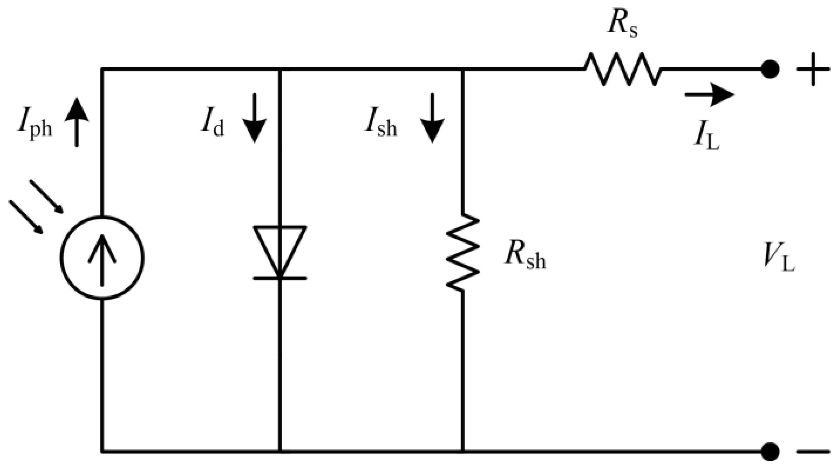
Single diode model is a very popular model used to simulate the I-V characteristic of a solar cell. The output current (A), as depicted in Figure 1, can be formulated as follows according to Kirchhoff’s current law.
where , , and are the photo generated current (A), diode current (A), and shunt resistor current (A), respectively. and are calculated by Equations (2) and (3), respectively [24,35,51,52,53].
where and represent the output voltage (V) and thermal voltage (V), respectively. is the reverse saturation current (A). and denote the series resistance (Ω) and shunt resistance (Ω), respectively. is the diode ideal factor. is the Boltzmann constant. is the electron charge. denotes the cell temperature in Kelvin.
Substituting Equations (2)–(4) into Equation (1), the output current can be written as follows:
It is observed from Equation (5) that if we know the values of , then the I-V characteristic of this model can be constructed. Therefore, accurate extraction of these five unknown parameters is the core of this study.
2.2. Double Diode Model
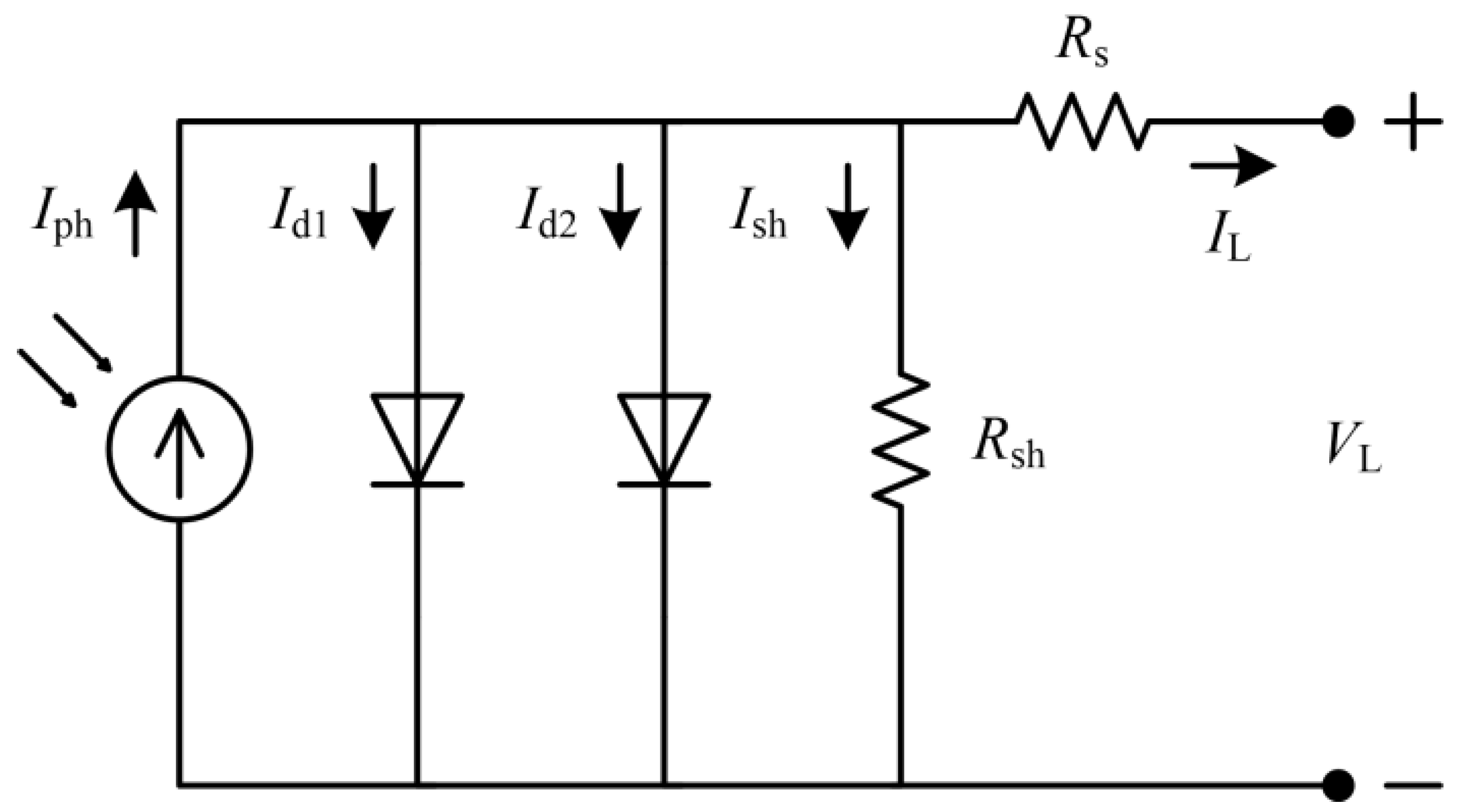
The above model performs well for almost all types of solar cells [5]. However, its performance is unsatisfactory at low irradiance for thin films based solar cells. The problem can be handled well by the double diode model [24,35]. The output current in Figure 2 is formulated as follows [52,54,55]:
where and represent the diffusion current (A) and saturation current (A), respectively. and are the diode ideal factors. Compared with the single diode mode, this model adds two more unknown parameters () and thereby the total number of unknown parameters that need to be extracted is seven ().
2.3. PV Module
2.4. Objective Function
Accurate extracted values for the involved unknown parameters of solar cell models should make the constructed model coincide with the real model. Namely, by using the constructed model, the calculated data should match the measured data well. Therefore, the difference between the measured current and the calculated current can be used to reflect the agreement degree. In general, the root mean square error (RMSE) is highly preferred [18,20,21,22,23,24,25].
where is the number of measured data and is the solution vector.
For the abovementioned three models, the objective functions and the solution vectors are as follows:
3. Symbiotic Organisms Search (SOS) Algorithm
SOS [48] is a young, yet effective metaheuristic inspired by the symbiotic interaction ways employed by organisms to improve their overall competitiveness in the ecosystem. Each organism (i.e., population individual) is represented as a D-dimensional vector , where , is the number of organisms in the ecosystem (i.e., population size). SOS contains mutualism, commensalism, and parasitism phases.
3.1. Mutualism Phase
In this phase, two organisms establish a good interaction relationship in which they can obtain what they need, and thus their mutual survival advantage can be increased simultaneously. For each organism of the ecosystem, a random distinct organism is selected to interact with by the following formulations:
where and are new candidate solutions for and , respectively. is a random number generated uniformly in (a,b). and are benefit factors with the random value 1 or 2. represents the best organism of the ecosystem. is the relationship characteristic.
3.2. Commensalism Phase
In this phase, two organisms build a unidirectional relationship where one organism benefits from the other organism as shown in Equation (14), whereas gets nothing from .
3.3. Parasitism Phase
In parasitism, one organism improves its survivability through harming the other organism . In SOS, this relationship is modeled as follows. An organism is copied and used to create an artificial parasite . Then, some random dimensions of are selected and modified by a random number generated within the corresponding bounds. The other organism , selected randomly from the ecosystem, serves as a host to the parasite . If is better than , then will be replaced by ; otherwise, will be discarded.
The pseudo-code of SOS is presented in Algorithm 1. It can be seen that apart from the common parameter, that is, the population size used in all metaheuristic algorithms, SOS has no algorithm-specific parameters that need to be well-tuned.
| Algorithm 1: The pseudo-code of SOS | |
| 1: | Initialize an ecosystem with organisms randomly |
| 2: | Calculate the fitness value of each organism |
| 3: | Set the iteration number |
| 4: | While the terminating criterion is not met do |
| 5: | Select the fittest organism of the ecosystem |
| 6: | For to do |
| 7: | /* mutualism phase */ |
| 8: | Select a random organism () from the ecosystem |
| 9: | Generate the i-th new organism using Equation (12) |
| 10: | Generate the j-th new organism using Equation (13) |
| 11: | Calculate the fitness value of and |
| 12: | Replace the old organism if it is defeated by the new one |
| 13: | /* commensalism phase */ |
| 14: | Select a random organism () from the ecosystem |
| 15: | Generate the i-th new organism using Equation (14) |
| 16: | Calculate the fitness value of |
| 17: | Replace the old organism if it is defeated by the new one |
| 18: | /* parasitism phase */ |
| 19: | Select a random organism () from the ecosystem |
| 20: | Generate an artificial parasite |
| 21: | Select a random number of dimensions of |
| 22: | Replace the selected dimensions using a random number |
| 23: | Calculate the fitness value of the modified |
| 24: | Replace if the modified is better than |
| 25: | End for |
| 26: | |
| 27: | End while |
4. Results and Discussions
4.1. Test PV Models
In this work, SOS is applied to three cases including single diode, double diode, and PV module models. The datasets are derived from the literature [58]. The measurements are conducted on an RTC France silicon solar cell and a Photowatt-PWP201 solar module. The former operates under 1000 W/m2 at 33 °C. The latter contains 36 polycrystalline silicon cells connected in series operating under 1000 W/m2 at 45 °C. The boundaries of extracted parameters are presented in Table 1.
4.2. Experimental Settings
In this work, the maximum number of fitness evaluations (Max_FEs), which is set to 50,000 [29], serves as the terminating criterion. In addition, to verify the effectiveness of SOS, five state-of-the-art algorithms including across neighborhood search (ANS) [59], biogeography-based learning particle swarm optimization (BLPSO) [60], competitive swarm optimizer (CSO) [61], chaotic teaching-learning algorithm (CTLA) [62], and levy flight trajectory-based whale optimization algorithm (LWOA) [63] are used for performance comparison. These five methods keep the original algorithm parameters, except the population size ps, setting the same unified value 50 for fair comparison. For each case, each method runs 50 times independently.
4.3. Experimental Results and Comparison
4.3.1. Results Comparison on the Single Diode Model
The experimental results of the first case are tabulated in Table 2. The symbols Min, Max, Mean, and Std. dev. represent the minimum, maximum, mean, and standard deviation values, respectively, over 50 independent runs. The experimental results of some well-designed methods, including SA [18] IADE [23], ABSO [24], GOTLBO [25], IJAYA [28], differential evolution (DE) [33], biogeography-based optimization algorithm with mutation strategies (BBO-M) [34], grouping-based global harmony search (GGHS) [35], chaotic asexual reproduction optimization (CARO) [40], bird mating optimizer (BMO) [44], and pattern search (PS) [45], are also provided in Table 2 for comparison. It can be seen that, compared with ANS, BLPSO, CSO, CTLA, and LWOA, SOS can acquire the lowest RMSE value (9.8609 × 10⁻⁴). Considering the mean, maximum, and standard deviation values, SOS also consistently performs better than them. In addition, SOS is also highly competitive against other recently proposed methods. It is better than IADE, ABSO, BBO-M, GGHS, GOTLBO, CARO, PS, and SA, except not better than DE, IJAYA, and BMO. Although DE, IJAYA, and BMO beat SOS, the disparities are very small.
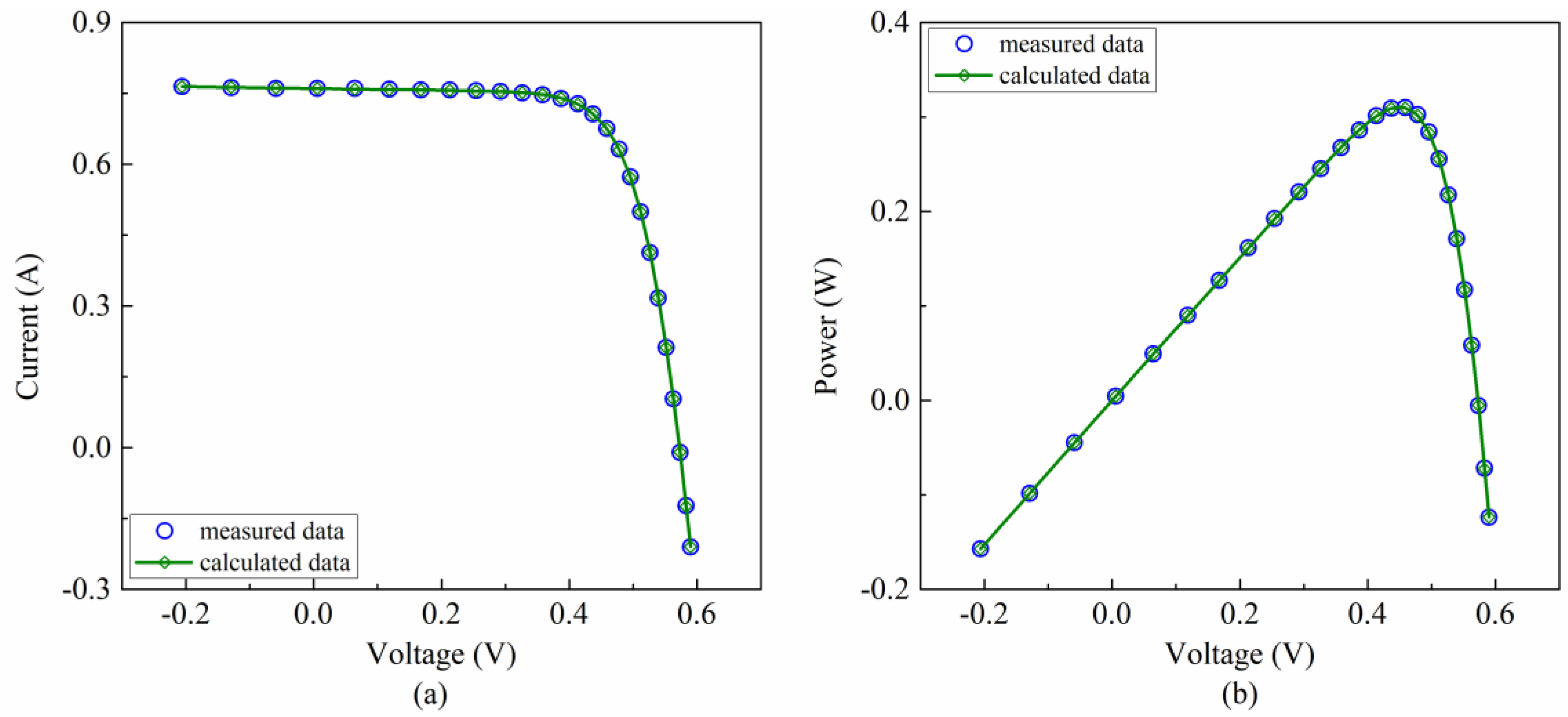
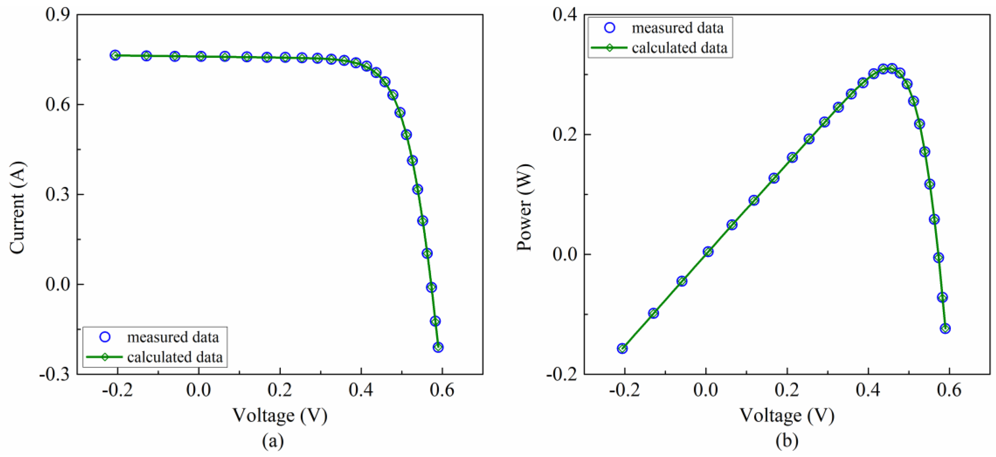
The best extracted values for the five unknown parameters of single diode model are given in Table 3. We observe that these listed methods almost extract close values for the unknown parameters. Utilizing the extracted parameters in Table 3, we reconstruct the characteristic curves as illustrated in Figure 3. We see that both the output current and power calculated by SOS match the measured values well throughout the whole range of voltage. In addition, we also tabulate the output current data calculated by ANS, BLPSO, CSO, CTLA, LWOA, and SOS in Table 4. An error index the sum of individual absolute error (SIAE) given in Equation (15) is used to evaluate the fitting error. It is obvious that the SIAE value of SOS is the smallest, followed by that of ANS, LWOA, BLPSO, CTLA, and CSO, meaning that SOS achieves more accurate values for the relevant parameters of single diode model.
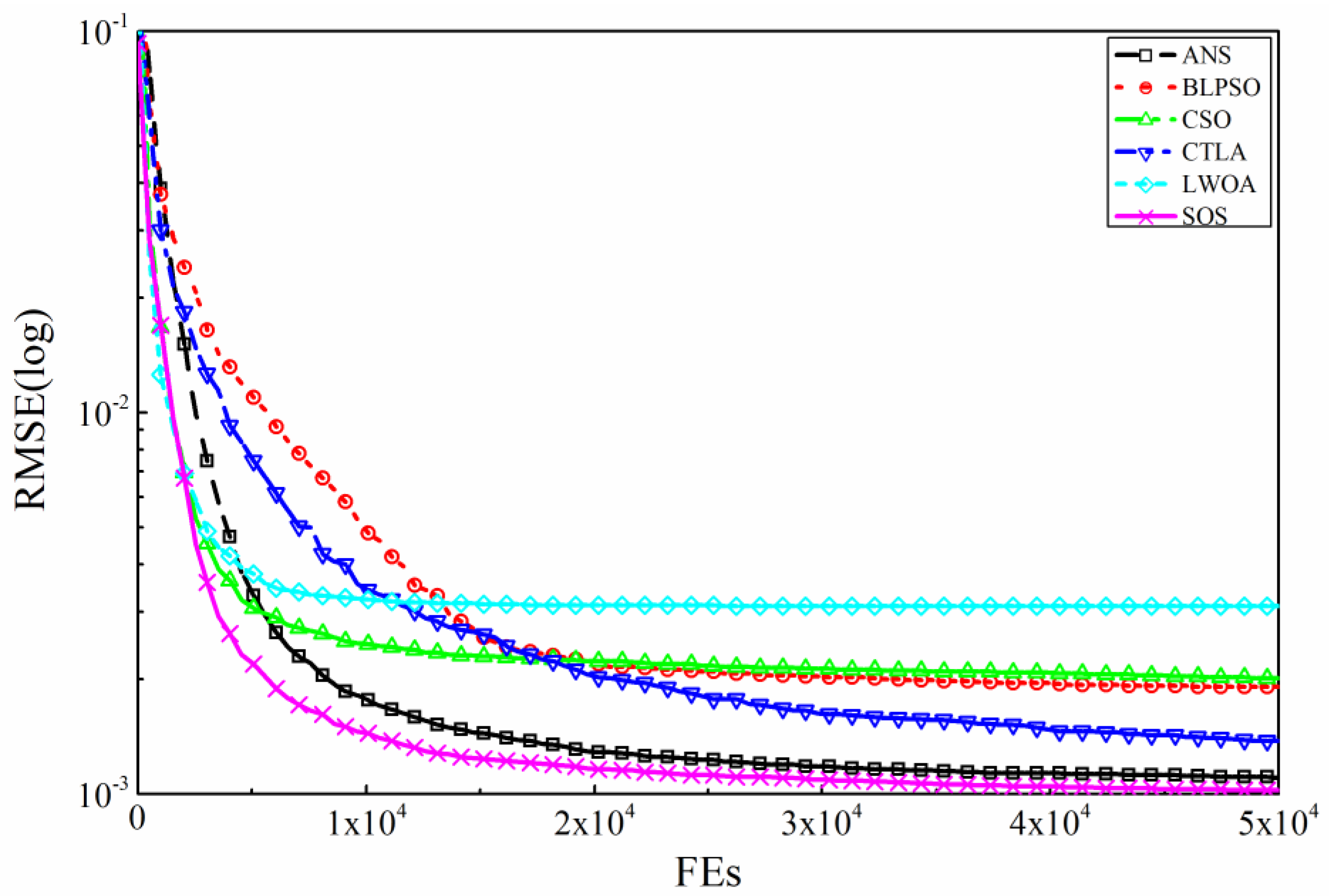
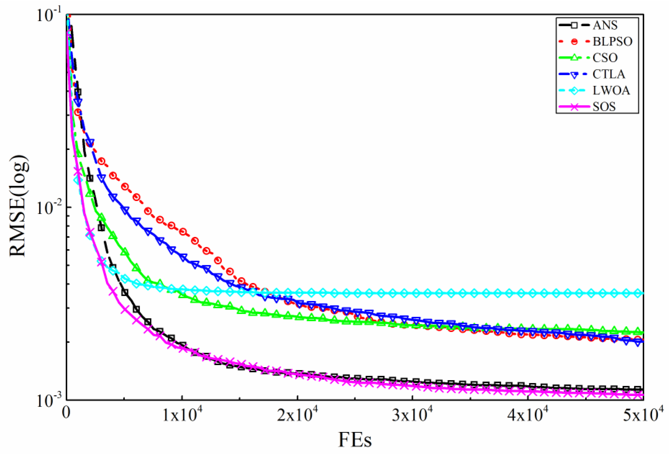
Besides, the convergence curves are presented in Figure 4. It is obvious that SOS is slightly slower than LWOA in the opening phase, however, the latter stagnates soon and then suffers from premature convergence, indicating that it has been caught in a local optimum. For the other four methods, SOS consistently converges faster than them throughout the whole evolutionary process.
4.3.2. Results Comparison on the Double Diode Model
The experimental results of the second case are summarized in Table 5. Similar to the comparison results on the single diode model, SOS performs better than ANS, BLPSO, CSO, CTLA, and LWOA in various RMSE indicators on the double diode model. SOS is surpassed by GOTLBO, CARO, and IJAYA, but it outperforms GGHS, PS, and SA. It is worth noting that the standard deviation value of SOS is the smallest among all compared methods, which indicates that SOS is highly robust. The extracted parameters are tabulated in Table 6. The reconstructed characteristic curves provided in Figure 5 clearly demonstrate that the calculated current and power achieved by SOS match up well with the measured values. The curve fitting results presented in Table 7 manifest once again that SOS can yield the smallest SIAE value (0.0182), followed by ANS, LWOA, BLPSO, CTLA, and CSO, which demonstrates the high accuracy of the parameters extracted by SOS for the double diode model. The convergence graph illustrated in Figure 6 reveals that SOS exhibits noticeably faster convergence rate than BLPSO, CSO, CTLA, and LWOA, but not ANS, which is slightly faster than SOS during the intermediate stage. However, ANS is surpassed by SOS in other stages.
4.3.3. Results Comparison on the PV Module Model
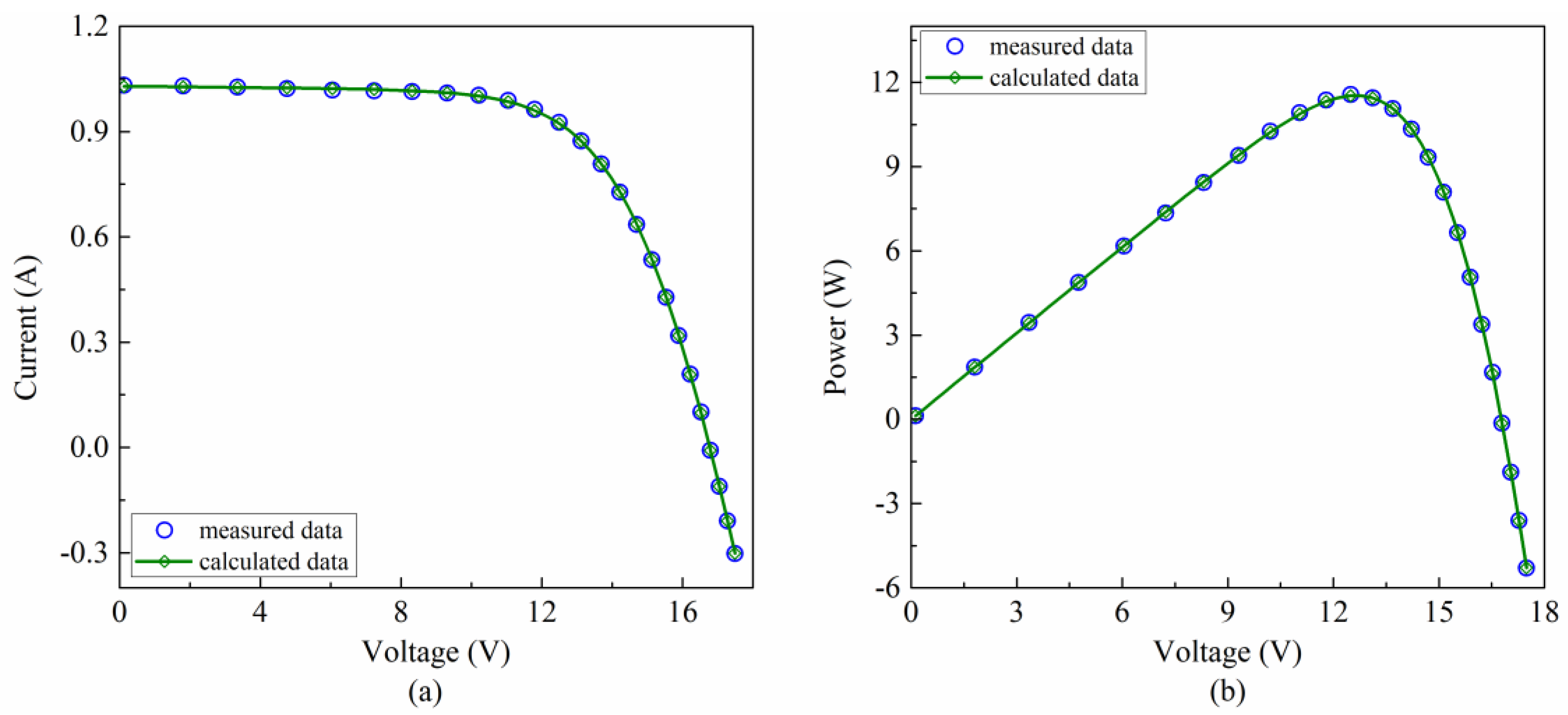
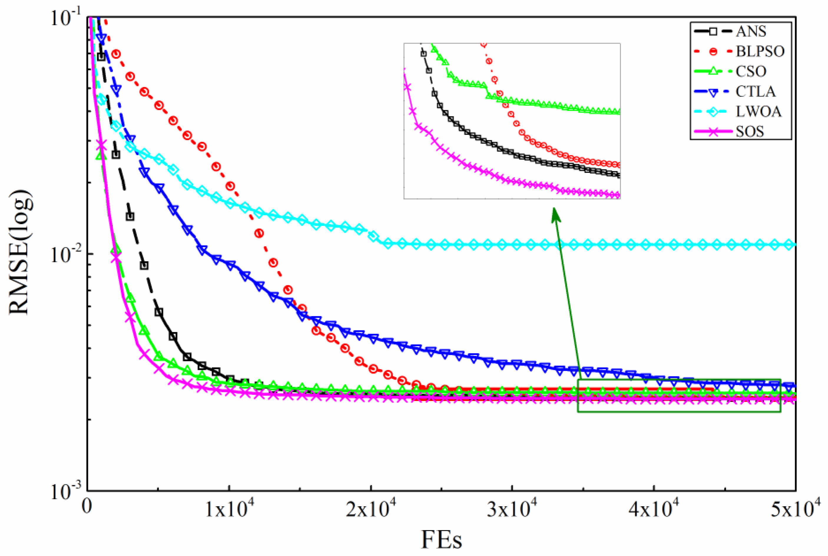
The RMSE values of the third case listed in Table 8 indicate that SOS, together with IJAYA, can provide the smallest RMSE value (2.4251 × 10⁻³) among all methods. Based on the optimal extracted parameters in Table 9, the corresponding characteristic curves are rebuilt and illustrated in Figure 7. It is clear that the output current and power calculated by SOS are highly in coincidence with the measured values. The SIAE results presented in Table 10 repeatedly manifest that SOS can achieve the most accurate values for the unknown parameters, followed by ANS, BLPSO, LWOA, CTLA, and CSO. The curves presented in Figure 8 state clearly that SOS is consistently faster than its competitors from beginning to end.
4.3.4. Statistical Analysis
The significance difference between two methods can be measured by the statistical analysis. Wilcoxon’s rank sum test is a reliable and robust statistical analysis tool and is widely used in metaheuristic methods. In this paper, the Wilcoxon’s rank sum test at a 0.05 confidence level is used to identify the significance difference between SOS and other compared methods on the same case. The test results are tabulated in Table 11. The symbol “†” denotes that SOS is statistically better than its competitor. The results demonstrate that SOS significantly outperforms every method on every case (p < 0.05), indicating the better performance of SOS from another perspective.
5. Conclusions and Future Work
The SOS algorithm is applied to solve the parameter extraction problem of solar cell models in this paper. To validate the effectiveness of SOS, it is applied to three models including single diode model, double diode model, and PV module models. From the comparison results of SOS with five state-of-the-art algorithms, namely, ANS, BLPSO, CSO, CTLA, and LWOA, it is summarized that SOS can extract more accurate and robust values for the unknown parameters with a faster convergence rate. The superiority of SOS is also demonstrated through statistical analysis based on the Wilcoxon’s rank sum test. In addition, the feasibility of SOS is further confirmed through comparison with some well-designed parameter extraction methods and it indicates that SOS is highly competitive. Meanwhile, there is still room for improvement for SOS to achieve more accurate values, especially for the double diode model. In summary, SOS behaves potential effectively in solving the parameter extraction problem of solar cell models. In future, some advanced strategies such as orthogonal learning and hybridization will be employed to further improve its performance.
Author Contributions
G.X. developed the idea behind the present research and wrote the manuscript. J.Z. provided theoretical analysis. X.Y. and D.S. contributed to final review and manuscript corrections. Y.H. collaborated in processing the experimental data.
Funding
This research was funded by the National Natural Science Foundation of China (Grant No. 51867005, 51667007), the Scientific Research Foundation for the Introduction of Talent of Guizhou University (Grant No. [2017]16), the Guizhou Education Department Growth Foundation for Youth Scientific and Technological Talents (Grant No. QianJiaoHe KY Zi [2018]108), the Guizhou Province Science and Technology Innovation Talent Team Project (Grant No. [2018]5615), the Science and Technology Foundation of Guizhou Province (Grant No. [2016]1036), and the Key Science and Technology Projects of China Southern Power Grid Co., Ltd. (Grant No. GZKJQQ00000417).
Conflicts of Interest
The authors declare no conflict of interest.
Nomenclature
| AP | artificial parasite |
| BF1, BF2 | benefit factors determined randomly as either 1 or 2 |
| D | dimension of individual vector |
| Id | diode current (A) |
| IL | output current (A) |
| Iph | photo generated current (A) |
| Isd, Isd1, Isd2 | saturation currents (A) |
| Ish | shunt resistor current (A) |
| k | Boltzmann constant (1.3806503 × 10⁻²³ J/K) |
| n, n1, n2 | diode ideality factors |
| Max_FEs | maximum number of fitness evaluations |
| N | number of experimental data |
| Np | number of cells connected in parallel |
| Ns | number of cells connected in series |
| ps | size of population |
| q | electron charge (1.60217646 × 10⁻¹⁹ C) |
| rand(a,b) | uniformly distributed random real number in (a,b) |
| Rs | series resistance (Ω) |
| Rsh | shunt resistance (Ω) |
| t | current iteration |
| T | cell temperature (K) |
| VL | output voltage (V) |
| Vt | diode thermal voltage (V) |
| x | extracted parameters vector |
| xi,d | dth parameter of ith organism |
| Xi | ith organism |
| Xbest | best organism found so far |
| I-V | current-voltage |
| P-V | power-voltage |
| PV | photovoltaic |
| RMSE | root mean square error |
| SIAE | sum of individual absolute error |
| Min | minimum RMSE |
| Max | maximum RMSE |
| Mean | mean RMSE |
| Std Dev | standard deviation |
| ABSO | artificial bee swarm optimization |
| ANS | across neighborhood search |
| BBO-M | biogeography-based optimization algorithm with mutation strategies |
| BLPSO | biogeography-based learning particle swarm optimization |
| BMO | bird mating optimizer |
| CARO | chaotic asexual reproduction optimization |
| CSO | competitive swarm optimizer |
| CTLA | chaotic teaching-learning algorithm |
| DE | differential evolution |
| GGHS | grouping-based global harmony search |
| GOTLBO | generalized oppositional teaching learning based optimization |
| IADE | improved adaptive DE |
| IJAYA | improved JAYA |
| LWOA | levy flight trajectory-based whale optimization algorithm |
| PS | pattern search |
| SOS | symbiotic organisms search |
| SA | simulated annealing |
References
- SolarPower Europe. SolarPower Europe’s Global Solar Market Outlook for Solar Power 2018–2022: Solar Growth Ahead; SolarPower Europe: Brussels, Belgium, 2018. [Google Scholar]
- China Energy Net. Available online: http://www.china5e.com (accessed on 5 September 2018).
- International Energy Agency. World Energy Outlook 2017; International Energy Agency: Paris, France, 2017. [Google Scholar]
- Youssef, A.; El-Telbany, M.; Zekry, A. The role of artificial intelligence in photo-voltaic systems design and control: A review. Renew. Sustain. Energy Rev. 2017, 78, 72–79. [Google Scholar] [CrossRef]
- Chin, V.J.; Salam, Z.; Ishaque, K. Cell modelling and model parameters estimation techniques for photovoltaic simulator application: A review. Appl. Energy 2015, 154, 500–519. [Google Scholar] [CrossRef]
- Jordehi, A.R. Parameter estimation of solar photovoltaic (PV) cells: A review. Renew. Sustain. Energy Rev. 2016, 61, 354–371. [Google Scholar] [CrossRef]
- Rhouma, M.B.H.; Gastli, A.; Brahim, L.B.; Touati, F.; Benammar, M. A simple method for extracting the parameters of the PV cell single-diode model. Renew. Energy 2017, 113, 885–894. [Google Scholar] [CrossRef]
- Batzelis, E.I.; Papathanassiou, S.A. A Method for the Analytical Extraction of the Single-Diode PV Model Parameters. IEEE Trans. Sustain. Energy 2016, 7, 504–512. [Google Scholar] [CrossRef]
- Brano, V.L.; Ciulla, G. An efficient analytical approach for obtaining a five parameters model of photovoltaic modules using only reference data. Appl. Energy 2013, 111, 894–903. [Google Scholar] [CrossRef]
- Louzazni, M.; Aroudam, E.H. An analytical mathematical modeling to extract the parameters of solar cell from implicit equation to explicit form. Appl. Sol. Energy 2015, 51, 165–171. [Google Scholar] [CrossRef]
- Kumar, G.; Panchal, A.K. A non-iterative technique for determination of solar cell parameters from the light generated I-V characteristic. J. Appl. Phys. 2013, 114, 84903. [Google Scholar] [CrossRef]
- Saleem, H.; Karmalkar, S. An Analytical Method to Extract the Physical Parameters of a Solar Cell from Four Points on the Illuminated J-V Curve. IEEE Electr. Device Lett. 2009, 30, 349–352. [Google Scholar] [CrossRef]
- Wang, G.; Zhao, K.; Shi, J.; Chen, W.; Zhang, H.; Yang, X.; Zhao, Y. An iterative approach for modeling photovoltaic modules without implicit equations. Appl. Energy 2017, 202, 189–198. [Google Scholar] [CrossRef]
- Wolf, P.; Benda, V. Identification of PV solar cells and modules parameters by combining statistical and analytical methods. Sol. Energy 2013, 93, 151–157. [Google Scholar] [CrossRef]
- Toledo, F.J.; Blanes, J.M. Analytical and quasi-explicit four arbitrary point method for extraction of solar cell single-diode model parameters. Renew. Energy 2016, 92, 346–356. [Google Scholar] [CrossRef]
- Yeh, W.C.; Huang, C.L.; Lin, P.; Chen, Z.; Jiang, Y.; Sun, B. Simplex Simplified Swarm Optimization for the Efficient Optimization of Parameter Identification for Solar Cell Models. IET Renew. Power Gener. 2018, 12, 45–51. [Google Scholar] [CrossRef]
- Bastidasrodriguez, J.D.; Petrone, G.; Ramospaja, C.A.; Spagnuolo, G. A genetic algorithm for identifying the single diode model parameters of a photovoltaic panel. Math. Comput. Simul. 2017, 131, 38–54. [Google Scholar] [CrossRef]
- El-Naggar, K.M.; Alrashidi, M.R.; Alhajri, M.F.; Al-Othman, A.K. Simulated Annealing algorithm for photovoltaic parameters identification. Sol. Energy 2012, 86, 266–274. [Google Scholar] [CrossRef]
- Bana, S.; Saini, R.P. Identification of unknown parameters of a single diode photovoltaic model using particle swarm optimization with binary constraints. Renew. Energy 2017, 101, 1299–1310. [Google Scholar] [CrossRef]
- Nunes, H.G.G.; Pombo, J.A.N.; Mariano, S.J.P.S.; Calado, M.R.A.; Souza, J.A.M.F. A new high performance method for determining the parameters of PV cells and modules based on guaranteed convergence particle swarm optimization. Appl. Energy 2018, 211, 774–791. [Google Scholar] [CrossRef]
- Ishaque, K.; Salam, Z.; Mekhilef, S.; Shamsudin, A. Parameter extraction of solar photovoltaic modules using penalty-based differential evolution. Appl. Energy 2012, 99, 297–308. [Google Scholar] [CrossRef]
- Chellaswamy, C.; Ramesh, R. Parameter extraction of solar cell models based on adaptive differential evolution algorithm. Renew. Energy 2016, 97, 823–837. [Google Scholar] [CrossRef]
- Jiang, L.L.; Maskell, D.L.; Patra, J.C. Parameter estimation of solar cells and modules using an improved adaptive differential evolution algorithm. Appl. Energy 2013, 112, 185–193. [Google Scholar] [CrossRef]
- Askarzadeh, A.; Rezazadeh, A. Artificial bee swarm optimization algorithm for parameters identification of solar cell models. Appl. Energy 2013, 102, 943–949. [Google Scholar] [CrossRef]
- Chen, X.; Yu, K.; Du, W.; Zhao, W.; Liu, G. Parameters identification of solar cell models using generalized oppositional teaching learning based optimization. Energy 2016, 99, 170–180. [Google Scholar] [CrossRef]
- Chen, X.; Xu, B.; Mei, C.; Ding, Y.; Li, K. Teaching–learning–based artificial bee colony for solar photovoltaic parameter estimation. Appl. Energy 2018, 212, 1578–1588. [Google Scholar] [CrossRef]
- Yu, K.; Chen, X.; Wang, X.; Wang, Z. Parameters identification of photovoltaic models using self-adaptive teaching-learning-based optimization. Energy Convers. Manag. 2017, 145, 233–246. [Google Scholar] [CrossRef]
- Yu, K.; Liang, J.J.; Qu, B.Y.; Chen, X.; Wang, H.; Yu, K. Parameters identification of photovoltaic models using an improved JAYA optimization algorithm. Energy Convers. Manag. 2017, 150, 742–753. [Google Scholar] [CrossRef]
- Yu, K.; Liang, J.J.; Qu, B.Y.; Cheng, Z.; Wang, H. Multiple learning backtracking search algorithm for estimating parameters of photovoltaic models. Appl. Energy 2018, 226, 408–422. [Google Scholar] [CrossRef]
- Oliva, D.; Aziz, M.A.E.; Hassanien, A.E. Parameter estimation of photovoltaic cells using an improved chaotic whale optimization algorithm. Appl. Energy 2017, 200, 141–154. [Google Scholar] [CrossRef]
- Oliva, D.; Ewees, A.A.; Aziz, M.A.E.; Hassanien, A.E.; Cisneros, M.P. A Chaotic Improved Artificial Bee Colony for Parameter Estimation of Photovoltaic Cells. Energies 2017, 10, 865. [Google Scholar] [CrossRef]
- Kichou, S.; Silvestre, S.; Guglielminotti, L.; Mora-López, L.; Muñoz-Cerón, E. Comparison of two PV array models for the simulation of PV systems using five different algorithms for the parameters identification. Renew. Energy 2016, 99, 270–279. [Google Scholar] [CrossRef]
- Ma, J.; Bi, Z.; Ting, T.O.; Hao, S.; Hao, W. Comparative performance on photovoltaic model parameter identification via bio-inspired algorithms. Sol. Energy 2016, 132, 606–616. [Google Scholar] [CrossRef]
- Niu, Q.; Zhang, L.; Li, K. A biogeography-based optimization algorithm with mutation strategies for model parameter estimation of solar and fuel cells. Energy Convers. Manag. 2014, 86, 1173–1185. [Google Scholar] [CrossRef]
- Askarzadeh, A.; Rezazadeh, A. Parameter identification for solar cell models using harmony search-based algorithms. Sol. Energy 2012, 86, 3241–3249. [Google Scholar] [CrossRef]
- Valdivia-González, A.; Zaldívar, D.; Cuevas, E.; Pérez-Cisneros, M.; Fausto, F.; González, A. A Chaos-Embedded Gravitational Search Algorithm for the Identification of Electrical Parameters of Photovoltaic Cells. Energies 2017, 7, 1052. [Google Scholar] [CrossRef]
- Rezk, H.; Fathy, A. A novel optimal parameters identification of triple-junction solar cell based on a recently meta-heuristic water cycle algorithm. Sol. Energy 2017, 157, 778–791. [Google Scholar] [CrossRef]
- Alam, D.F.; Yousri, D.A.; Eteiba, M.B. Flower Pollination Algorithm based solar PV parameter estimation. Energy Convers. Manag. 2015, 101, 410–422. [Google Scholar] [CrossRef]
- Ali, E.E.; El-Hameed, M.A.; El-Fergany, A.A.; El-Arini, M.M. Parameter extraction of photovoltaic generating units using multi-verse optimizer. Sustain. Energy Technol. Assess. 2016, 17, 68–76. [Google Scholar] [CrossRef]
- Yuan, X.; He, Y.; Liu, L. Parameter extraction of solar cell models using chaotic asexual reproduction optimization. Neural Comput. Appl. 2015, 26, 1227–1239. [Google Scholar] [CrossRef]
- Babu, T.S.; Ram, J.P.; Sangeetha, K.; Laudani, A.; Rajasekar, N. Parameter extraction of two diode solar PV model using Fireworks algorithm. Sol. Energy 2016, 140, 265–276. [Google Scholar] [CrossRef]
- Allam, D.; Yousri, D.A.; Eteiba, M.B. Parameters extraction of the three diode model for the multi-crystalline solar cell/module using Moth-Flame Optimization Algorithm. Energy Convers. Manag. 2016, 123, 535–548. [Google Scholar] [CrossRef]
- Fathy, A.; Rezk, H. Parameter estimation of photovoltaic system using imperialist competitive algorithm. Renew. Energy 2017, 111, 307–320. [Google Scholar] [CrossRef]
- Askarzadeh, A.; Rezazadeh, A. Extraction of maximum power point in solar cells using bird mating optimizer-based parameters identification approach. Sol. Energy 2013, 90, 123–133. [Google Scholar] [CrossRef]
- Alhajri, M.F.; El-Naggar, K.M.; Alrashidi, M.R.; Al-Othman, A.K. Optimal extraction of solar cell parameters using pattern search. Renew. Energy 2012, 44, 238–245. [Google Scholar] [CrossRef]
- Xiong, G.; Zhang, J.; Shi, D.; He, Y. Parameter extraction of solar photovoltaic models using an improved whale optimization algorithm. Energy Convers. Manag. 2018, 174, 388–405. [Google Scholar] [CrossRef]
- Wolpert, D.H.; Macready, W.G. No free lunch theorems for optimization. IEEE Trans. Evol. Comput. 1997, 1, 67–82. [Google Scholar] [CrossRef] [Green Version]
- Cheng, M.Y.; Prayogo, D. Symbiotic Organisms Search: A new metaheuristic optimization algorithm. Comput. Struct. 2014, 139, 98–112. [Google Scholar] [CrossRef]
- Saha, S.; Mukherjee, V. A novel chaos-integrated symbiotic organisms search algorithm for global optimization. Soft Comput. 2018, 22, 3797–3816. [Google Scholar] [CrossRef]
- Panda, A.; Pani, S. A Symbiotic Organisms Search algorithm with adaptive penalty function to solve multi-objective constrained optimization problems. Appl. Soft Comput. 2016, 46, 344–360. [Google Scholar] [CrossRef]
- Shongwe, S.; Hanif, M. Comparative Analysis of Different Single-Diode PV Modeling Methods. IEEE J. Photovolt. 2015, 5, 938–946. [Google Scholar] [CrossRef]
- Humada, A.M.; Hojabri, M.; Mekhilef, S.; Hamada, H.M. Solar cell parameters extraction based on single and double-diode models: A review. Renew. Sustain. Energy Rev. 2016, 56, 494–509. [Google Scholar] [CrossRef]
- Deihimi, M.H.; Naghizadeh, R.A.; Meyabadi, A.F. Systematic derivation of parameters of one exponential model for photovoltaic modules using numerical information of data sheet. Renew. Energy 2016, 87, 676–685. [Google Scholar] [CrossRef]
- Jordehi, A.R. Maximum power point tracking in photovoltaic (PV) systems: A review of different approaches. Renew. Sustain. Energy Rev. 2016, 65, 1127–1138. [Google Scholar] [CrossRef]
- Ishaque, K.; Salam, Z.; Taheri, H. Simple, fast and accurate two-diode model for photovoltaic modules. Sol. Energy Mater. Sol. Cells 2011, 95, 586–594. [Google Scholar] [CrossRef]
- Awadallah, M.A. Variations of the bacterial foraging algorithm for the extraction of PV module parameters from nameplate data. Energy Convers. Manag. 2016, 113, 312–320. [Google Scholar] [CrossRef]
- Chen, Z.; Wu, L.; Cheng, S.; Lin, P.; Wu, Y.; Lin, W. Intelligent fault diagnosis of photovoltaic arrays based on optimized kernel extreme learning machine and I-V characteristics. Appl. Energy 2017, 204, 912–931. [Google Scholar] [CrossRef]
- Easwarakhanthan, T.; Bottin, J.; Bouhouch, I.; Boutrit, C. Nonlinear minimization algorithm for determining the solar cell parameters with microcomputers. Int. J. Sol. Energy 1986, 4, 1–12. [Google Scholar] [CrossRef]
- Wu, G. Across neighborhood search for numerical optimization. Inform. Sci. 2016, 329, 597–618. [Google Scholar] [CrossRef] [Green Version]
- Chen, X.; Tianfield, H.; Mei, C.; Du, W.; Liu, G. Biogeography-based learning particle swarm optimization. Soft Comput. 2017, 21, 7519–7541. [Google Scholar] [CrossRef]
- Cheng, R.; Jin, Y. A competitive swarm optimizer for large scale optimization. IEEE Trans. Cybern. 2015, 42, 191–204. [Google Scholar] [CrossRef] [PubMed]
- Farah, A.; Guesmi, T.; Abdallah, H.H.; Ouali, A. A novel chaotic teaching-learning-based optimization algorithm for multi-machine power system stabilizers design problem. Int. J. Electr. Power 2016, 77, 197–209. [Google Scholar] [CrossRef]
- Ling, Y.; Zhou, Y.; Luo, Q. Lévy flight trajectory-based whale optimization algorithm for global optimization. IEEE Access 2017, 5, 6168–6186. [Google Scholar] [CrossRef]
Figure 1.
Single diode model.

Figure 2.
Double diode model.

Figure 3.
Extraction results by SOS for the single diode model. (a) Current; (b) power.

Figure 4.
Convergence curves for the single diode model.

Figure 5.
Extraction results by SOS for the double diode model. (a) Current; (b) power.

Figure 6.
Convergence curves for the double diode model.

Figure 7.
Extraction results by SOS for the photovoltaic (PV) module model. (a) Current; (b) power.

Figure 8.
Convergence curves for the PV module model.


Table 1.
Parameter boundaries of solar cell models.
| Parameter | Single/Double Diode Model | PV Module Model | ||
|---|---|---|---|---|
| Lower Bound | Upper Bound | Lower Bound | Upper Bound | |
| Iph (A) | 0 | 1 | 0 | 2 |
| Isd (µA) | 0 | 1 | 0 | 50 |
| Rs (Ω) | 0 | 0.5 | 0 | 2 |
| Rsh (Ω) | 0 | 100 | 0 | 2000 |
| n, n1, n2 | 1 | 2 | 1 | 50 |
Table 2.
RMSE results for the single diode model.
| Method | Min | Max | Mean | Std. Dev. |
|---|---|---|---|---|
| IADE | 9.8900 × 10⁻⁴ | NA | NA | NA |
| ABSO | 9.9124 × 10⁻⁴ | NA | NA | NA |
| BBO-M | 9.8634 × 10⁻⁴ | NA | NA | NA |
| GGHS | 9.9078 × 10⁻⁴ | NA | NA | NA |
| GOTLBO | 9.87442 × 10⁻⁴ | 1.98244 × 10⁻³ | 1.33488 × 10⁻³ | 2.99407 × 10⁻⁴ |
| CARO | 9.8665 × 10⁻⁴ | NA | NA | NA |
| DE | 9.8602 × 10⁻⁴ | NA | NA | NA |
| IJAYA | 9.8603 × 10⁻⁴ | 1.0622 × 10⁻³ | 9.9204 × 10⁻⁴ | 1.4033 × 10⁻⁵ |
| BMO | 9.8608 × 10⁻⁴ | NA | NA | NA |
| PS | 2.863 × 10⁻¹ | NA | NA | NA |
| SA | 1.70 × 10⁻³ | NA | NA | NA |
| ANS | 9.9689 × 10⁻⁴ | 1.4385 × 10⁻³ | 1.1051 × 10⁻³ | 1.0141 × 10⁻⁴ |
| BLPSO | 1.4836 × 10⁻³ | 2.2415 × 10⁻³ | 1.9092 × 10⁻³ | 1.7404 × 10⁻⁴ |
| CSO | 1.6358 × 10⁻³ | 2.4104 × 10⁻³ | 2.0058 × 10⁻³ | 1.7398 × 10⁻⁴ |
| CTLA | 1.0991 × 10⁻³ | 1.8027 × 10⁻³ | 1.3772 × 10⁻³ | 1.7132 × 10⁻⁴ |
| LWOA | 1.0873 × 10⁻³ | 9.1622 × 10⁻³ | 3.1119 × 10⁻³ | 1.8838 × 10⁻³ |
| SOS | 9.8609 × 10⁻⁴ | 1.1982 × 10⁻³ | 1.0245 × 10⁻³ | 5.2184 × 10⁻⁵ |
NA: Not available in the literature.
Table 3.
xtracted parameters for the single diode model.
| Method | Iph (A) | Isd (µA) | Rs (Ω) | Rsh (Ω) | n | RMSE |
|---|---|---|---|---|---|---|
| IADE | 0.7607 | 0.33613 | 0.03621 | 54.7643 | 1.4852 | 9.8900 × 10⁻⁴ |
| ABSO | 0.76080 | 0.30623 | 0.03659 | 52.2903 | 1.47583 | 9.9124 × 10⁻⁴ |
| BBO-M | 0.76078 | 0.31874 | 0.03642 | 53.36277 | 1.47984 | 9.8634 × 10⁻⁴ |
| GGHS | 0.76092 | 0.32620 | 0.03631 | 53.0647 | 1.48217 | 9.9079 × 10⁻⁴ |
| GOTLBO | 0.760780 | 0.331552 | 0.036265 | 54.115426 | 1.483820 | 9.8744 × 10⁻⁴ |
| CARO | 0.76079 | 0.31724 | 0.03644 | 53.0893 | 1.48168 | 9.8665 × 10⁻⁴ |
| DE | 0.7608 | 0.323 | 0.0364 | 53.719 | 1.4812 | 9.8602 × 10⁻⁴ |
| IJAYA | 0.7608 | 0.3228 | 0.0364 | 53.7595 | 1.4811 | 9.8603 × 10⁻⁴ |
| PS | 0.7617 | 0.9980 | 0.0313 | 64.1026 | 1.6000 | 2.863 × 10⁻¹ |
| SA | 0.7620 | 0.4798 | 0.0345 | 43.1034 | 1.5172 | 1.70 × 10⁻³ |
| ANS | 0.7607 | 0.3407 | 0.0362 | 54.7917 | 1.4866 | 9.9689 × 10⁻⁴ |
| BLPSO | 0.7599 | 0.4977 | 0.0347 | 96.5115 | 1.5257 | 1.4836 × 10⁻³ |
| CSO | 1.0205 | 0.3658 | 1.2122 | 1689.0050 | 48.8206 | 1.6358 × 10⁻³ |
| CTLA | 0.7650 | 0.4280 | 0.0357 | 61.1131 | 1.5092 | 1.0991 × 10⁻³ |
| LWOA | 1.0284 | 0.3145 | 1.2218 | 1272.0197 | 48.2413 | 1.0873 × 10⁻³ |
| SOS | 0.7608 | 0.3579 | 0.0359 | 53.7835 | 1.4916 | 9.8609 × 10⁻⁴ |
Table 4.
Fitting results for the single diode model.
| Item | VL (V) | IL Measured (A) | IL Calculated (A) | |||||
|---|---|---|---|---|---|---|---|---|
| ANS | BLPSO | CSO | CTLA | LWOA | SOS | |||
| 1 | −0.2057 | 0.7640 | 0.7639 | 0.7617 | 0.7614 | 0.7679 | 0.7631 | 0.7641 |
| 2 | −0.1291 | 0.7620 | 0.7625 | 0.7609 | 0.7606 | 0.7667 | 0.7618 | 0.7627 |
| 3 | −0.0588 | 0.7605 | 0.7613 | 0.7602 | 0.7598 | 0.7655 | 0.7607 | 0.7614 |
| 4 | 0.0057 | 0.7605 | 0.7601 | 0.7595 | 0.7591 | 0.7645 | 0.7597 | 0.7602 |
| 5 | 0.0646 | 0.7600 | 0.7590 | 0.7589 | 0.7585 | 0.7635 | 0.7587 | 0.7591 |
| 6 | 0.1185 | 0.7590 | 0.7580 | 0.7584 | 0.7579 | 0.7626 | 0.7578 | 0.7581 |
| 7 | 0.1678 | 0.7570 | 0.7571 | 0.7578 | 0.7573 | 0.7618 | 0.7570 | 0.7572 |
| 8 | 0.2132 | 0.7570 | 0.7561 | 0.7572 | 0.7567 | 0.7609 | 0.7561 | 0.7562 |
| 9 | 0.2545 | 0.7555 | 0.7551 | 0.7564 | 0.7559 | 0.7599 | 0.7552 | 0.7551 |
| 10 | 0.2924 | 0.7540 | 0.7537 | 0.7552 | 0.7546 | 0.7585 | 0.7538 | 0.7537 |
| 11 | 0.3269 | 0.7505 | 0.7514 | 0.7530 | 0.7524 | 0.7561 | 0.7517 | 0.7514 |
| 12 | 0.3585 | 0.7465 | 0.7473 | 0.7489 | 0.7484 | 0.7519 | 0.7477 | 0.7473 |
| 13 | 0.3873 | 0.7385 | 0.7400 | 0.7414 | 0.7412 | 0.7443 | 0.7406 | 0.7399 |
| 14 | 0.4137 | 0.7280 | 0.7273 | 0.7282 | 0.7288 | 0.7310 | 0.7280 | 0.7271 |
| 15 | 0.4373 | 0.7065 | 0.7068 | 0.7072 | 0.7091 | 0.7099 | 0.7076 | 0.7065 |
| 16 | 0.4590 | 0.6755 | 0.6751 | 0.6750 | 0.6789 | 0.6774 | 0.6759 | 0.6748 |
| 17 | 0.4784 | 0.6320 | 0.6306 | 0.6303 | 0.6369 | 0.6322 | 0.6315 | 0.6303 |
| 18 | 0.4960 | 0.5730 | 0.5719 | 0.5715 | 0.5812 | 0.5727 | 0.5726 | 0.5716 |
| 19 | 0.5119 | 0.4990 | 0.4994 | 0.4991 | 0.5119 | 0.4997 | 0.4999 | 0.4991 |
| 20 | 0.5265 | 0.4130 | 0.4134 | 0.4134 | 0.4288 | 0.4133 | 0.4137 | 0.4133 |
| 21 | 0.5398 | 0.3165 | 0.3173 | 0.3175 | 0.3342 | 0.3169 | 0.3173 | 0.3172 |
| 22 | 0.5521 | 0.2120 | 0.2122 | 0.2126 | 0.2292 | 0.2116 | 0.2120 | 0.2122 |
| 23 | 0.5633 | 0.1035 | 0.1029 | 0.1032 | 0.1181 | 0.1021 | 0.1026 | 0.1029 |
| 24 | 0.5736 | −0.0100 | −0.0091 | −0.0091 | −0.0025 | −0.0101 | −0.0094 | −0.0091 |
| 25 | 0.5833 | −0.1230 | −0.1243 | −0.1249 | −0.1180 | −0.1255 | −0.1245 | −0.1244 |
| 26 | 0.5900 | −0.2100 | −0.2092 | −0.2104 | −0.2078 | −0.2105 | −0.2092 | −0.2094 |
| SIAE | 0.0182 | 0.0275 | 0.1347 | 0.0739 | 0.0191 | 0.0181 | ||
Table 5.
RMSE results for the double diode model.
| Method | Min | Max | Mean | Std. dev. |
|---|---|---|---|---|
| GGHS | 9.8635 × 10⁻⁴ | NA | NA | NA |
| GOTLBO | 9.83177 × 10⁻⁴ | 1.78774 × 10⁻³ | 1.24360 × 10⁻³ | 2.09115 × 10⁻⁴ |
| CARO | 9.8260 × 10⁻⁴ | NA | NA | NA |
| IJAYA | 9.8293 × 10⁻⁴ | 1.4055 × 10⁻³ | 1.0269 × 10⁻³ | 9.8625 × 10⁻⁵ |
| PS | 1.5180 × 10⁻² | NA | NA | NA |
| SA | 1.9000 × 10⁻² | NA | NA | NA |
| ANS | 1.0042 × 10⁻³ | 1.4456 × 10⁻³ | 1.1337 × 10⁻³ | 9.9500 × 10⁻⁵ |
| BLPSO | 1.5704 × 10⁻³ | 2.5312 × 10⁻³ | 2.0554 × 10⁻³ | 2.0186 × 10⁻⁴ |
| CSO | 1.7013 × 10⁻³ | 2.7735 × 10⁻³ | 2.2421 × 10⁻³ | 2.2059 × 10⁻⁴ |
| CTLA | 1.3216 × 10⁻³ | 3.1002 × 10⁻³ | 2.0145 × 10⁻³ | 4.0895 × 10⁻⁴ |
| LWOA | 1.3120 × 10⁻³ | 1.3387 × 10⁻² | 3.5838 × 10⁻³ | 2.6270 × 10⁻³ |
| SOS | 9.8518 × 10⁻⁴ | 1.3498 × 10⁻³ | 1.0627 × 10⁻³ | 9.6141 × 10⁻⁵ |
NA: Not available in the literature.
Table 6.
Extracted parameters for the double diode model.
| Method | Iph (A) | Isd1 (µA) | Rs (Ω) | Rsh (Ω) | n1 | Isd2 (µA) | n2 | RMSE |
|---|---|---|---|---|---|---|---|---|
| GGHS | 0.76079 | 0.97310 | 0.03690 | 56.8368 | 1.92126 | 0.16791 | 1.42814 | 9.8635 × 10⁻⁴ |
| GOTLBO | 0.760752 | 0.800195 | 0.036783 | 56.075304 | 1.999973 | 0.220462 | 1.448974 | 9.83177 × 10⁻⁴ |
| CARO | 0.76075 | 0.29315 | 0.03641 | 54.3967 | 1.47338 | 0.09098 | 1.77321 | 9.8260 × 10⁻⁴ |
| IJAYA | 0.7601 | 0.0050445 | 0.0376 | 77.8519 | 1.2186 | 0.75094 | 1.6247 | 9.8293 × 10⁻⁴ |
| PS | 0.7602 | 0.9889 | 0.0320 | 81.3008 | 1.6000 | 0.0001 | 1.1920 | 1.5180 × 10⁻² |
| SA | 0.7623 | 0.4767 | 0.0345 | 43.1034 | 1.5172 | 0.0100 | 2.0000 | 1.9000 × 10⁻² |
| ANS | 0.7609 | 0.1785 | 0.0369 | 51.5905 | 1.8181 | 0.2466 | 1.4581 | 1.0042 × 10⁻³ |
| BLPSO | 0.7607 | 0.5481 | 0.0338 | 78.6922 | 1.5442 | 0.0542 | 1.5765 | 1.5704 × 10⁻³ |
| CSO | 0.7628 | 0.7954 | 0.0409 | 15.7733 | 1.6936 | 0.6780 | 1.8138 | 1.7013 × 10⁻³ |
| CTLA | 0.7570 | 0.8542 | 0.0313 | 89.6464 | 1.7879 | 0.3812 | 1.5230 | 1.3216 × 10⁻³ |
| LWOA | 0.7597 | 0.2342 | 0.0355 | 86.8763 | 1.4679 | 0.3709 | 1.6989 | 1.3120 × 10⁻³ |
| SOS | 0.7606 | 0.5408 | 0.0365 | 55.5537 | 1.9346 | 0.2418 | 1.4579 | 9.8518 × 10⁻⁴ |
Table 7.
Fitting results for the double diode model.
| Item | VL (V) | IL Measured (A) | IL Calculated (A) | |||||
|---|---|---|---|---|---|---|---|---|
| ANS | BLPSO | CSO | CTLA | LWOA | SOS | |||
| 1 | −0.2057 | 0.7640 | 0.7644 | 0.7630 | 0.7738 | 0.7591 | 0.7618 | 0.7638 |
| 2 | −0.1291 | 0.7620 | 0.7629 | 0.7620 | 0.7690 | 0.7582 | 0.7609 | 0.7625 |
| 3 | −0.0588 | 0.7605 | 0.7615 | 0.7611 | 0.7645 | 0.7574 | 0.7601 | 0.7612 |
| 4 | 0.0057 | 0.7605 | 0.7603 | 0.7603 | 0.7605 | 0.7567 | 0.7593 | 0.7600 |
| 5 | 0.0646 | 0.7600 | 0.7591 | 0.7595 | 0.7567 | 0.7561 | 0.7586 | 0.7590 |
| 6 | 0.1185 | 0.7590 | 0.7581 | 0.7588 | 0.7533 | 0.7554 | 0.7580 | 0.7580 |
| 7 | 0.1678 | 0.7570 | 0.7571 | 0.7581 | 0.7501 | 0.7548 | 0.7574 | 0.7571 |
| 8 | 0.2132 | 0.7570 | 0.7561 | 0.7574 | 0.7470 | 0.7541 | 0.7567 | 0.7561 |
| 9 | 0.2545 | 0.7555 | 0.7550 | 0.7565 | 0.7440 | 0.7532 | 0.7559 | 0.7551 |
| 10 | 0.2924 | 0.7540 | 0.7536 | 0.7552 | 0.7407 | 0.7518 | 0.7547 | 0.7536 |
| 11 | 0.3269 | 0.7505 | 0.7513 | 0.7528 | 0.7366 | 0.7494 | 0.7525 | 0.7513 |
| 12 | 0.3585 | 0.7465 | 0.7472 | 0.7485 | 0.7312 | 0.7449 | 0.7484 | 0.7472 |
| 13 | 0.3873 | 0.7385 | 0.7400 | 0.7407 | 0.7233 | 0.7369 | 0.7410 | 0.7399 |
| 14 | 0.4137 | 0.7280 | 0.7274 | 0.7273 | 0.7116 | 0.7234 | 0.7280 | 0.7271 |
| 15 | 0.4373 | 0.7065 | 0.7071 | 0.7060 | 0.6951 | 0.7023 | 0.7072 | 0.7066 |
| 16 | 0.4590 | 0.6755 | 0.6756 | 0.6737 | 0.6718 | 0.6704 | 0.6753 | 0.6750 |
| 17 | 0.4784 | 0.6320 | 0.6312 | 0.6290 | 0.6412 | 0.6265 | 0.6307 | 0.6307 |
| 18 | 0.4960 | 0.5730 | 0.5724 | 0.5704 | 0.6024 | 0.5689 | 0.5719 | 0.5720 |
| 19 | 0.5119 | 0.4990 | 0.4997 | 0.4984 | 0.5557 | 0.4979 | 0.4994 | 0.4995 |
| 20 | 0.5265 | 0.4130 | 0.4136 | 0.4133 | 0.5009 | 0.4136 | 0.4137 | 0.4136 |
| 21 | 0.5398 | 0.3165 | 0.3172 | 0.3178 | 0.4394 | 0.3185 | 0.3176 | 0.3174 |
| 22 | 0.5521 | 0.2120 | 0.2120 | 0.2133 | 0.3717 | 0.2137 | 0.2126 | 0.2123 |
| 23 | 0.5633 | 0.1035 | 0.1026 | 0.1041 | 0.3002 | 0.1034 | 0.1031 | 0.1029 |
| 24 | 0.5736 | −0.0100 | −0.0093 | −0.0082 | 0.2259 | −0.0105 | −0.0090 | −0.0091 |
| 25 | 0.5833 | −0.1230 | −0.1243 | −0.1241 | 0.1483 | −0.1289 | −0.1246 | −0.1243 |
| 26 | 0.5900 | −0.2100 | −0.2089 | −0.2098 | 0.0904 | −0.2168 | −0.2098 | −0.2091 |
| SIAE | 0.0189 | 0.0283 | 1.6176 | 0.0789 | 0.0247 | 0.0182 | ||
Table 8.
RMSE results for the photovoltaic (PV) module model.
| Method | Min | Max | Mean | Std. dev. |
|---|---|---|---|---|
| CARO | 2.427 × 10⁻³ | NA | NA | NA |
| IJAYA | 2.4251 × 10⁻³ | 2.4393 × 10⁻³ | 2.4289 × 10⁻³ | 3.7755 × 10⁻⁶ |
| PS | 1.18 × 10⁻² | NA | NA | NA |
| SA | 2.70 × 10⁻³ | NA | NA | NA |
| ANS | 2.4310 × 10⁻³ | 2.5658 × 10⁻³ | 2.4702 × 10⁻³ | 2.9121 × 10⁻⁵ |
| BLPSO | 2.4296 × 10⁻³ | 2.5616 × 10⁻³ | 2.4884 × 10⁻³ | 3.3055 × 10⁻⁵ |
| CSO | 2.4537 × 10⁻³ | 3.0650 × 10⁻³ | 2.5804 × 10⁻³ | 7.7274 × 10⁻⁵ |
| CTLA | 2.4782 × 10⁻³ | 3.5579 × 10⁻³ | 2.7760 × 10⁻³ | 2.4714 × 10⁻⁴ |
| LWOA | 2.6352 × 10⁻³ | 6.7023 × 10⁻² | 1.0936 × 10⁻² | 1.3115 × 10⁻² |
| SOS | 2.4251 × 10⁻³ | 2.5103 × 10⁻³ | 2.4361 × 10⁻³ | 1.7503 × 10⁻⁵ |
NA: Not available in the literature.
Table 9.
Extracted parameters for the PV module model.
| Method | Iph (A) | Isd (µA) | Rs (Ω) | Rsh (Ω) | n | RMSE |
|---|---|---|---|---|---|---|
| CARO | 1.03185 | 3.28401 | 1.20556 | 841.3213 | 48.40363 | 2.427 × 10⁻³ |
| IJAYA | 1.0305 | 3.4703 | 1.2016 | 977.3752 | 48.6298 | 2.4251 × 10⁻³ |
| PS | 1.0313 | 3.1756 | 1.2053 | 714.2857 | 48.2889 | 1.18 × 10⁻² |
| SA | 1.0331 | 3.6642 | 1.1989 | 833.3333 | 48.8211 | 2.7000 × 10⁻³ |
| ANS | 1.0301 | 3.6650 | 1.1967 | 1070.4564 | 48.8377 | 2.4310 × 10⁻³ |
| BLPSO | 1.0302 | 3.6462 | 1.1964 | 1029.5378 | 48.8198 | 2.4296 × 10⁻³ |
| CSO | 1.0205 | 3.6578 | 1.2122 | 1689.0050 | 48.8206 | 2.4537 × 10⁻³ |
| CTLA | 1.0248 | 2.6365 | 1.2689 | 1722.6637 | 47.5838 | 2.4782 × 10⁻³ |
| LWOA | 1.0284 | 3.1435 | 1.2218 | 1272.0197 | 48.2413 | 2.6352 × 10⁻³ |
| SOS | 1.0303 | 3.5616 | 1.1991 | 1017.7000 | 48.7291 | 2.4251 × 10⁻³ |
Table 10.
Fitting results for the PV module model.
| Item | VL (V) | IL Measured (A) | IL Calculated (A) | |||||
|---|---|---|---|---|---|---|---|---|
| ANS | BLPSO | CSO | CTLA | LWOA | SOS | |||
| 1 | 0.1248 | 1.0315 | 1.0288 | 1.0289 | 1.0197 | 1.0240 | 1.0273 | 1.0289 |
| 2 | 1.8093 | 1.0300 | 1.0272 | 1.0272 | 1.0187 | 1.0230 | 1.0259 | 1.0272 |
| 3 | 3.3511 | 1.0260 | 1.0257 | 1.0257 | 1.0177 | 1.0220 | 1.0246 | 1.0256 |
| 4 | 4.7622 | 1.0220 | 1.0241 | 1.0241 | 1.0166 | 1.0210 | 1.0233 | 1.0241 |
| 5 | 6.0538 | 1.0180 | 1.0224 | 1.0223 | 1.0154 | 1.0198 | 1.0218 | 1.0223 |
| 6 | 7.2364 | 1.0155 | 1.0201 | 1.0200 | 1.0135 | 1.0180 | 1.0198 | 1.0199 |
| 7 | 8.3189 | 1.0140 | 1.0166 | 1.0164 | 1.0103 | 1.0151 | 1.0165 | 1.0164 |
| 8 | 9.3097 | 1.0100 | 1.0108 | 1.0106 | 1.0047 | 1.0098 | 1.0110 | 1.0105 |
| 9 | 10.2163 | 1.0035 | 1.0009 | 1.0007 | 0.9951 | 1.0006 | 1.0014 | 1.0007 |
| 10 | 11.0449 | 0.9880 | 0.9848 | 0.9846 | 0.9792 | 0.9850 | 0.9857 | 0.9847 |
| 11 | 11.8018 | 0.9630 | 0.9598 | 0.9596 | 0.9542 | 0.9603 | 0.9609 | 0.9597 |
| 12 | 12.4929 | 0.9255 | 0.9230 | 0.9229 | 0.9175 | 0.9235 | 0.9242 | 0.9230 |
| 13 | 13.1231 | 0.8725 | 0.8725 | 0.8724 | 0.8668 | 0.8726 | 0.8736 | 0.8725 |
| 14 | 13.6983 | 0.8075 | 0.8072 | 0.8071 | 0.8014 | 0.8064 | 0.8080 | 0.8072 |
| 15 | 14.2221 | 0.7265 | 0.7278 | 0.7277 | 0.7220 | 0.7261 | 0.7283 | 0.7279 |
| 16 | 14.6995 | 0.6345 | 0.6363 | 0.6363 | 0.6305 | 0.6337 | 0.6364 | 0.6364 |
| 17 | 15.1346 | 0.5345 | 0.5356 | 0.5356 | 0.5299 | 0.5323 | 0.5353 | 0.5357 |
| 18 | 15.5311 | 0.4275 | 0.4288 | 0.4288 | 0.4234 | 0.4252 | 0.4281 | 0.4288 |
| 19 | 15.8929 | 0.3185 | 0.3186 | 0.3187 | 0.3137 | 0.3154 | 0.3179 | 0.3187 |
| 20 | 16.2229 | 0.2085 | 0.2079 | 0.2079 | 0.2034 | 0.2053 | 0.2071 | 0.2079 |
| 21 | 16.5241 | 0.1010 | 0.0984 | 0.0984 | 0.0945 | 0.0970 | 0.0978 | 0.0984 |
| 22 | 16.7987 | −0.0080 | −0.0082 | −0.0081 | −0.0114 | −0.0081 | −0.0085 | −0.0081 |
| 23 | 17.0499 | −0.1110 | −0.1110 | −0.1110 | −0.1135 | −0.1093 | −0.1109 | −0.1109 |
| 24 | 17.2793 | −0.2090 | −0.2092 | −0.2092 | −0.2110 | −0.2056 | −0.2087 | −0.2091 |
| 25 | 17.4885 | −0.3030 | −0.3021 | −0.3021 | −0.3032 | −0.2966 | −0.3011 | −0.3020 |
| SIAE | 0.0423 | 0.0424 | 0.1380 | 0.0646 | 0.0452 | 0.0421 | ||
Table 11.
Statistical analysis results based on Wilcoxon’s rank sum.
| SOS Vs. | Single Diode Model | Double Diode Model | PV Module Model |
|---|---|---|---|
| ANS | † (p = 2.3044 × 10⁻⁸) | † (p = 3.4341 × 10⁻⁶) | † (p = 5.5646 × 10⁻¹²) |
| BLPSO | † (p = 7.0661 × 10⁻¹⁸) | † (p = 7.0661 × 10⁻¹⁸) | † (p = 9.9263 × 10⁻¹⁴) |
| CSO | † (p = 7.0661 × 10⁻¹⁸) | † (p = 7.0661 × 10⁻¹⁸) | † (p = 8.9852 × 10⁻¹⁸) |
| CTLA | † (p = 2.1975 × 10⁻¹⁷) | † (p = 7.5041 × 10⁻¹⁸) | † (p = 9.5403 × 10⁻¹⁸) |
| LWOA | † (p = 1.2866 × 10⁻¹⁷) | † (p = 8.4620 × 10⁻¹⁸) | † (p = 7.0661 × 10⁻¹⁸) |
© 2018 by the authors. Licensee MDPI, Basel, Switzerland. This article is an open access article distributed under the terms and conditions of the Creative Commons Attribution (CC BY) license (http://creativecommons.org/licenses/by/4.0/).
Share and Cite
MDPI and ACS Style
Xiong, G.; Zhang, J.; Yuan, X.; Shi, D.; He, Y. Application of Symbiotic Organisms Search Algorithm for Parameter Extraction of Solar Cell Models. Appl. Sci. 2018, 8, 2155. https://0-doi-org.brum.beds.ac.uk/10.3390/app8112155
AMA Style
Xiong G, Zhang J, Yuan X, Shi D, He Y. Application of Symbiotic Organisms Search Algorithm for Parameter Extraction of Solar Cell Models. Applied Sciences. 2018; 8(11):2155. https://0-doi-org.brum.beds.ac.uk/10.3390/app8112155
Chicago/Turabian StyleXiong, Guojiang, Jing Zhang, Xufeng Yuan, Dongyuan Shi, and Yu He. 2018. "Application of Symbiotic Organisms Search Algorithm for Parameter Extraction of Solar Cell Models" Applied Sciences 8, no. 11: 2155. https://0-doi-org.brum.beds.ac.uk/10.3390/app8112155
Note that from the first issue of 2016, this journal uses article numbers instead of page numbers. See further details here.