A High-Resolution Texture Mapping Technique for 3D Textured Model
by
 , and
, and
Jiing-Yih Lai
1,*, 
Tsung-Chien Wu
1,
Watchama Phothong
1,
Douglas W. Wang
2,
Chao-Yaug Liao
1 and
Ju-Yi Lee
1 1
Department of Mechanical Engineering, National Central University, Taoyuan 32001, Taiwan
2
Ortery Technologies, Inc., New Taipei City 22052, Taiwan
*
Author to whom correspondence should be addressed.
Appl. Sci. 2018, 8(11), 2228; https://0-doi-org.brum.beds.ac.uk/10.3390/app8112228
Submission received: 1 October 2018
/
Revised: 1 November 2018
/
Accepted: 8 November 2018
/
Published: 12 November 2018
(This article belongs to the Special Issue Intelligent Imaging and Analysis)
Abstract
:We proposed a texture mapping technique that comprises mesh partitioning, mesh parameterization and packing, texture transferring, and texture correction and optimization for generating a high-quality texture map of a three-dimensional (3D) model for applications in e-commerce presentations. The main problems in texture mapping are that the texture resolution is generally worse than in the original images and considerable photo inconsistency exists at the transition of different image sources. To improve the texture resolution, we employed an oriented boundary box method for placing mesh islands on the parametric (UV) map. We also provided a texture size that can keep the texture resolution of the 3D textured model similar to that of the object images. To improve the photo inconsistency problem, we employed a method to detect and overcome the missing color that might exist on a texture map. We also proposed a blending process to minimize the transition error caused by different image sources. Thus, a high-quality 3D textured model can be obtained by applying this series of processes for presentations in e-commerce.
1. Introduction
Two-dimensional (2D) images are commonly used for product presentations in e-commerce because they can reveal the object’s texture and are easy to process. However, as 2D images can display only limited views of an object, it may be possible to capture hundreds of 2D images and orient an image at any viewing angle via a web viewer [1]. However, storing and displaying so many images while maintaining high image quality would have huge memory requirements. In addition, the actual three-dimensional (3D) shape and dimensions of an object cannot be obtained in this representation. 3D image-modeling technology is a technique for reconstructing the 3D model of an object by using multiple 2D images while maintaining its texture on the model (called 3D textured model hereafter). If its texture quality can be comparable to that of 2D images, this technology could be used to replace 2D images for product presentations, because a 3D textured model requires less memory and can freely be oriented in 3D space.
Product presentation usually requires a dedicated photography device to catch high-quality object images with known position and orientation in 3D space. The object images can be obtained using a single-camera device that applies a digital single-lens reflex (DSLR) camera to capture an object placed on a turntable, or a multi-camera device that applies several DSLR cameras mounted on an arm to capture an object placed on a turntable from different angles. These devices can position the camera precisely such that the camera information can be calibrated. The object on the turntable can also be oriented to capture object images in different views. These devices also provide a controlled environment, for example, single background color and adjustable lighting, such that the object images and the background color can easily be separated. As these devices are already used in the field of product presentation, we use them as the image source of the 3D-image modeling technology.
3D image-modeling technology primarily involves the generation of two kinds of information, the 3D model of an object and its texture map. The former employs triangular meshes to describe the object’s surface geometry, and the latter describes its color information. There is a mapping between the 3D model and the texture map such that when the model is displayed in 3D space, accurate object texture can be displayed accordingly. Approaches to generating 3D models from multiple images can be classified into two groups: shape-from-silhouette (SFS) and shape-from-photoconsistency (SFP). The SFP approach has received extensive attention because it can simultaneously yield a 3D geometric model of an object and its texture map. The main idea of this method is to generate photo-consistent models that can reduce some measure of the discrepancy between different image projections of their surface vertices [2,3,4]. The main advantage of the SFP approach is that it can generate fine surface details by using photometric and geometric information. However, the reliability of the SFP approach remains a problem because the texture quality can easily be affected by environmental factors such as noise in the colors, inaccuracies in camera calibration, non-Lambertian surfaces, and homogeneous object color.
However, the SFS approach is a common method used to estimate an object’s shape from images of its silhouettes [5,6,7]. This method is essentially based on a visual hull concept in which the object’s shape is constructed by the intersection of multiple sets of polygons from the silhouettes of multiple 2D images. With a sufficient number of images from different views, this method can yield an approximate model to describe the outline shape of an object. However, this model is not yet suitable for visualization due to the following two reasons. First, the SFS method can produce visual features on the 3D model, such as sharp edges and artifacts, which do not exist on the real object surface; some virtual features may be sufficient large to affect the outline shape. Second, concavities on the object surface are often formed as convex shapes because these are invisible on image silhouettes. Therefore, a quality improvement method must be implemented to remove virtual features while recovering the smoothness of the model [8]. The removal of artifacts is particularly important because they are difficult to detect and eliminate.
Texture mapping generally includes multiple techniques, such as mesh partitioning, mesh parameterization, texture transferring, and correction and optimization, which are related to each other and affect the texture quality. Research in mesh partitioning can be summarized using several different approaches. Shamir [9] categorized several methods of mesh partitioning according to segmentation type, partitioning technique, and segmentation criterion. Segmentation type refers to surface-type and part-type. Surface-type mesh partitioning is commonly used in texture mapping [10,11,12] because it can prevent large distortion in mesh parameterization. Mangan et al. [13,14] and Lavoué et al. [15] proposed a constant curvature watershed method to separate a mesh model into several regions. Other applications of surface-type partitioning include remeshing and simplification [16], mesh morphing, and mesh collision detection [17]. Part-type mesh partitioning is commonly used for part recognition on a mesh model composed of multiple parts. Mortara et al. [18,19] proposed a partitioning method by applying the curvature information at the transition of different parts to decompose a mesh model. Funkhouser et al. [20] proposed another method by establishing the database of some known parts for the separation of a mesh model. Partitioning techniques include region growing, hierarchical clustering, iterative clustering, and inferring from a skeleton, which can be implemented either alone or together. Segmentation criterion approaches include dihedral angle or normal angle, geodesic distance, and topological relationship, which can also be implemented either alone or together.
Mesh parameterization was classified in accordance with distortion minimization, boundary condition, and numerical complexity [21,22]. Distortion minimization can be summarized based on three types: angle, area, and distance. For angle minimization, an objective function is formulated to minimize the distortion of 2D meshes on the UV domain. Several methods can be employed for angle minimization. Lévy et al. [11] proposed a least-squares approximation of the Cauchy-Riemann equations to minimize both angle and area distortion on 2D meshes. Desbrun et al. [23] presented an instinct parameterization to minimize angle distortion. These two methods allow free boundaries and linear numerical complexity. Sheffer et al. [24] optimized the angles on the UV domain based on angle-base flattening. This method sets constraints on the topology of triangular meshes to preserve the correctness of 2D meshes. Sheffer et al. [25] proposed a hierarchical algorithm to improve the optimization efficiency for the case of huge triangular meshes, and Zayer et al. [26] proposed a method to solve the optimization problem for a set of linear equations that were derived based on the angle-base flattening approach with a set of constraints specified. In addition, the barycentric mapping is commonly used for mapping 3D meshes onto the UV domain in mesh processing. Tutte [27,28] proposed an algorithm to embed a 3D mesh onto the UV domain by evaluating the barycentric position in terms of its neighboring meshes. Eck et al. [29] proposed an algorithm to calculate the multiresolution form of a mesh via a barycentric map. Floater [30] applied a “shape-preserve” condition for the barycentric map to preserve the shape of 2D meshes on the UV domain. Floater [31] and Floater et al. [32] further applied mean-value weights for the barycentric map to preserve the shape of 2D meshes. For all above-mentioned barycentric mapping, the boundary is fixed and the numerical complexity is linear, which is not suitable for texture editing. For texture mapping, a method of free boundary is more appropriate as it can ensure that the boundary of each island of 2D meshes is close to the real profile, making the texture editing easy. Some other approaches have focused on minimizing the area distortion [33] and distance [34].
For texture map generation, the main idea is to deal with the texture transferring problem. Niem et al. [35] proposed a texture transferring method by identifying the most appropriate image source for a group of meshes. They also minimized the color inconsistency at the transition of two different groups and synthesized the invisible meshes using the color of neighboring pixels. Genç et al. [36] proposed a method to extract and render the texture dynamically. The extraction was implemented by horizontally scanning the pixels and rendering every color onto the meshes. Baumberg [37] proposed a blending method to handle the color difference between two different images. The images were separated into high and low bands; the low band images were averaged to minimize the color difference, whereas the high band images were kept to preserve the outline profile. In addition, texture synthesizing is commonly used to improve the transition between different textures. Efros et al. [38] proposed an image quilting method to quilt together different texture patterns. They extended the boundary of each original pattern and calculated the minimum color difference on the overlapping area to find the new boundary between two patterns. Wei et al. [39] proposed an algorithm to synthesize the texture pattern based on deterministic searching and use tree-structured vector quantization to improve the efficiency. These two approaches focus mainly on the transition synthesis between two texture patterns.
2. Problem Statement
For product presentations in e-commerce, texture quality is the most crucial issue to investigate because it directly affects the visualization effect. Ideally, the texture quality at any view in 3D space should perfectly match that of the corresponding 2D image. Actual texture on the 3D model, however, is usually worse than that of 2D images, mainly because individual texture on the 3D model comes from different image sources. A 3D model reconstructed using multiple images of an object is only an approximation of the object geometry. The camera model and calibration method used to estimate the camera parameters might yield additional errors in the position and orientation of the object images. These errors, combined with errors caused by the texture mapping process, might lead to discrepancy between the texture of the 3D model and the real object. Any defect in the 3D texture could negatively impact perceptions of the product being presented.
The following are typical problems involving the 3D texture:
- Reduced texture resolution: The texture resolution at any view in 3D space is worse than that of the corresponding object image, primarily because of inappropriate scaling of the pixels between the real image domain and the texture mapping image domain.
- Missing color on some mesh regions: All 2D meshes on the texture domain should ideally be color-filled, but some may be missed if they are beyond the boundary of the object image, primarily because of insufficient accuracy of the 3D model, especially for those meshes near the image silhouette.
- Photo inconsistency at the transition of different image sources: Photo inconsistency usually occurs along the boundary of different groups of meshes, with each group textured by different image sources. This problem is the combined effect of insufficient accuracy of the 3D model and the camera parameters.
Thus, we develop a texture mapping algorithm that focuses on detecting and removing these problems.
The objective of this study is to develop a high-quality texture mapping algorithm that can be combined with a 3D modeling algorithm to generate the 3D textured model of an object for use in e-commerce product presentation. High-quality texture here indicates that the texture at any view in 3D space should be as close as possible to that of the corresponding 2D image, which mainly requires maintenance of the resolution on the texture and elimination of photo-inconsistent errors at the transition of different image sources. A general texture mapping process comprising the following three techniques is proposed: mesh partitioning, mesh parameterization and packing, and texture transferring. Specific efforts are made at each step to initially eliminate problems that might affect the texture of the 3D model. To further reduce the discrepancy of the texture owing to insufficient inaccuracy of the 3D model and camera parameters, a correction and optimization algorithm is presented. The entire texture mapping process is fully automatic and is intended to be used for all kinds of objects.
The main contribution of the proposed texture mapping method is as follows. First, we enhance the techniques of converting 3D meshes onto the UV domain so that the shape of most 2D meshes can be preserved and the finest resolution can be obtained in texture transferring. Three main techniques in converting 3D meshes onto the UV domain are mesh partitioning, mesh parameterization and packing. In the proposed mesh partitioning algorithm, a novel chart growth method is proposed to partition 3D meshes iteratively so that each chart of 3D meshes can be as flat (disk type) as possible, which can reduce the error of 2D meshes in mesh parameterization. In the proposed mesh parameterization algorithm, a novel conformal mapping method is proposed to preserve the shape of 2D meshes as close to that of 3D meshes as possible. In the proposed packing method, all regions of 2D meshes are tightly packed in a rectangular area to acquire the finest resolution. Second, we propose an optimized texture transferring algorithm for generating the texture map, emphasizing the elimination of erroneous texture mapping owing to insufficient accuracy of the 3D model as well camera parameters, and the improvement of the texture resolution as close to that of 2D object images as possible. The strategies used in the proposed algorithm include: (1) increase overall texture size in pixels; (2) increase the number of pixels occupied by each 2D mesh; (3) detect and fill in void meshes; and (4) perform texture blending at the boundaries of mesh islands. The first two operations can improve the resolution of the final texture map, whereas the last two operations can eliminate erroneous texture mapping. Several realistic examples are presented to verify the feasibility of the proposed texture mapping method. The results are also compared with those form commercial software.
3. Overview of the Proposed Method
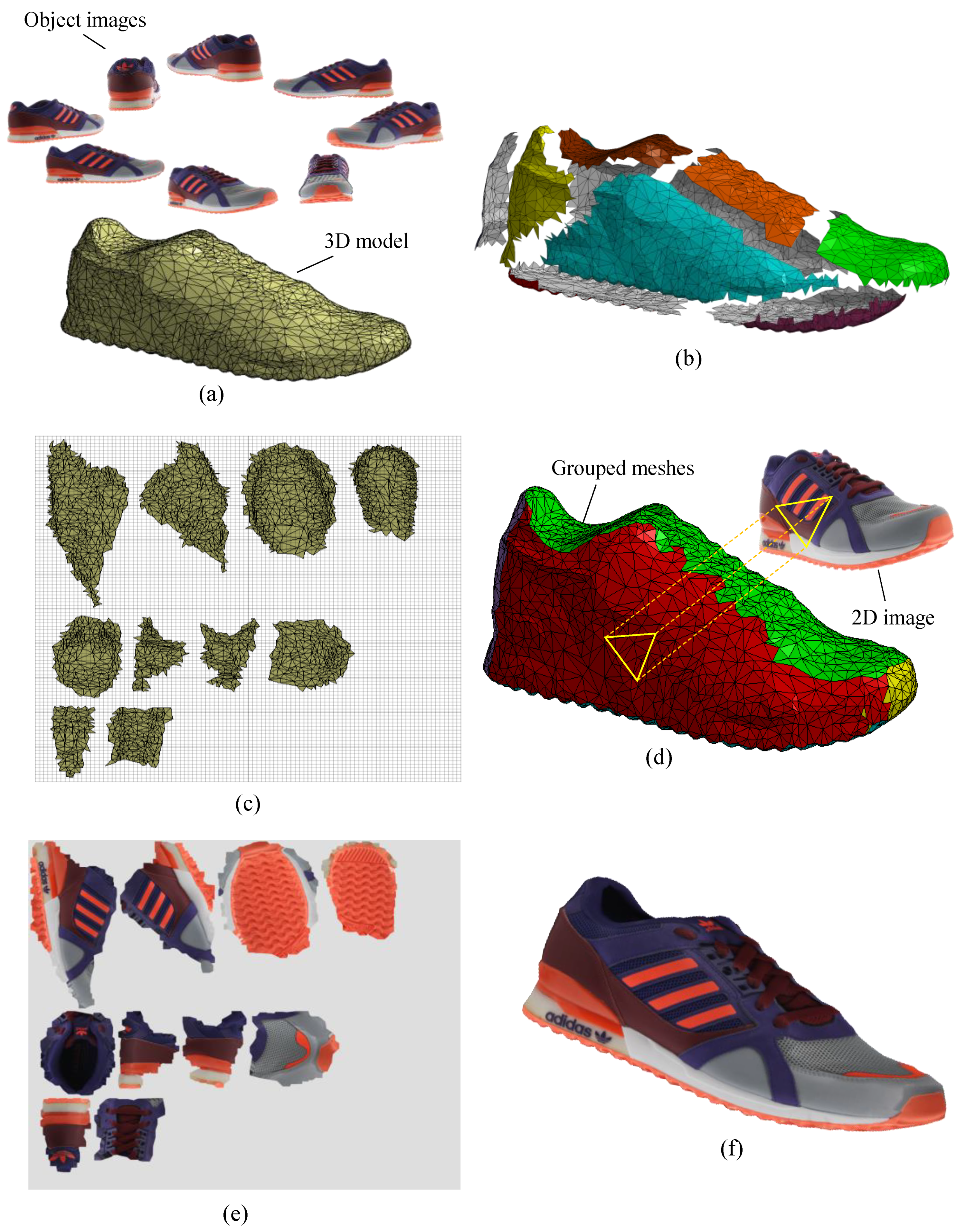
The 3D textured model is created by covering a 3D model with a texture map that stores the color information of the object. The main idea of direct texture mapping is to generate the texture of the 3D model by directly using the object images. Figure 1 shows the overall flowchart of the proposed texture mapping method. The input data are the 3D model of an object and multiple object images from different views (Figure 1a). The original 3D model was generated from silhouettes of the object images using an SFS method. However, the surface quality of the original meshes was not satisfactory because of artifacts and virtual features affecting the outline shape, as well as the surface smoothness. A mesh optimization algorithm combining re-meshing, mesh smoothing, and mesh reduction was employed to eliminate the effect of the above-mentioned phenomena and yield an optimized mesh model [8]. The model after mesh optimization served as the input of the proposed texture mapping algorithm.
In the proposed texture mapping algorithm, mesh partitioning is first implemented to subdivide the 3D model into several charts (Figure 1b), each of which is later individually mapped onto the UV domain. Mesh partitioning is based on a chart growth method to assign a weight to each mesh on the model, and grow each chart of meshes one by one from a set of initial seed meshes. The seed meshes are optimized in an iteration process until all meshes have been clustered. This ensures that all charts are flat and compact in the boundary for easy mapping in the mesh parameterization. Mesh parameterization and packing is then implemented to map the meshes on each chart and to pack all 2D meshes on the UV domain (Figure 1c). An angle-preserving algorithm is proposed to optimize the mapping between the 3D and 2D domains, which can preserve the shape of most 2D meshes. Furthermore, all 2D meshes are tightly packed in a rectangular area to acquire the finest resolution when mapping the pixels from the image domain to the texture domain.
Next, texture transferring is implemented to extract pixels from the image domain, and place them on the texture domain appropriately (Figure 1d). This procedure comprises three main steps: grouping the 3D meshes, extracting pixels from the image domain, and placing pixels onto the texture domain. We also propose a method to analyze the texture resolution. The proposed texture transferring algorithm ensures that the texture resolution can be set to the equivalent of the 2D images. Finally, we implement correction and optimization of the texture to eliminate erroneous color mapping that might occur due to the insufficient accuracy of the 3D model and camera parameters and to improve the photo consistency at the boundary of different image sources (Figure 1e). Several photo inconsistent problems are detected and solved one by one. The output texture map is saved as a universal data format (*.obj), which can be displayed with a website viewer (Figure 1f).
4. The Proposed Texture Mapping Method
4.1. Mesh Partitioning
The purpose of mesh partitioning is to partition 3D meshes into several charts, where a chart denotes a group of meshes that are tightly connected to each other and form a boundary loop only. When a chart is mostly flat and compact in boundaries, it is easy to preserve the shape in mesh parameterization. By contrast, when a chart is bent too much or closed on both sides, that is, two boundary loops, the shape distortion in the mesh parameterization increases, thereby reducing the texture resolution in some regions. A conventional approach to dealing with this issue is to map each mesh on the 3D model onto the UV domain independently, which can accurately preserve the shape of all 2D meshes and pack them all tightly row by row [40]. However, this approach might result in an un-editable texture map, because all 2D meshes are independently projected and distributed irregularly.
The proposed mesh partitioning technique essentially assigns a cost to each mesh, which denotes a mesh’s weight calculated by considering the flatness and distance of the mesh with respect to a chart. An iterative procedure combining chart growth and seed mesh upgrades is implemented to expand and modify charts as well as seed meshes in sequence. The chart growth is a process to cluster all meshes into charts in accordance with each mesh’s cost. When a closed chart is detected as possibly occurring, a new seed mesh is added to separate the chart into two. The seed mesh upgrading is a process to upgrade the seed mesh of each chart that has been expanded. Whenever a chart is grown, its seed mesh is recomputed by putting it near the center of the new chart.
Two costs are defined and used in chart growth and seed mesh upgrading. The cost used in chart growth is defined as
where denotes the weight of a candidate mesh neighboring a chart C, is the neighboring mesh of that has been in C, is the normal vector of C evaluated by the average of all normal vectors of the meshes in C, is the normal vector of the candidate mesh, and and are the centroids of and F, respectively. Equation (1) indicates that the cost considers both the flatness and distance of with respect to the chart C. The cost used in seed mesh upgrading is defined as
which is used to determine the mesh F that is closest to the candidate mesh .
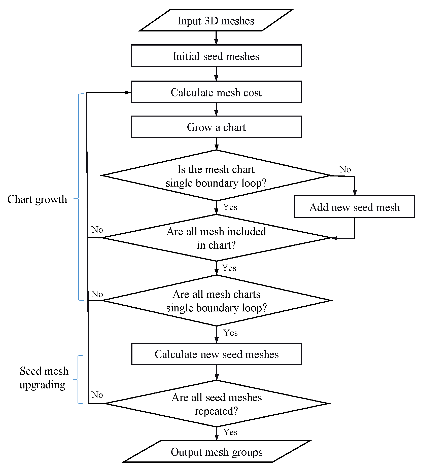
Figure 2 depicts the flowchart of the proposed mesh partitioning algorithm, which has three main steps: initial seed meshes, chart growth, and seed mesh upgrading. In step 1, a set of seed meshes are initially assigned on the input 3D meshes. A default value of 10 is typically used and the seed meshes are randomly selected from the 3D meshes. Each seed mesh is initially assigned as a chart.
In step 2, chart growth, all meshes neighboring the charts are found by using the topological data of the mesh model. Equation (1) is then employed to evaluate a cost for each of these meshes. The costs are sorted from minimum to maximum. The mesh with the minimum cost is selected to cluster with its neighboring chart. Three criteria are then checked in sequence. First, is this chart (which has just grown) a single boundary loop? If yes, go to the next criterion. If not, a new seed mesh is added. The last mesh added to this chart is regarded as the new seed mesh. Second, are all meshes clustered into charts? If yes, go to the next criterion. If not, go back to the beginning of this step. Third, are all charts a single boundary loop? If yes, this step is finished. If not, go back to the beginning of this step. Notably, after step 2, all meshes are clustered into charts.
In step 3, seed mesh upgrading, the seed mesh on each chart is recomputed. The upgraded seed mesh is located near the center of the chart, which is achieved by a reverse searching process from the boundary of the chart. Starting from a mesh on the boundary, Equation (2) is repeatedly employed to find a loop of meshes around the boundary of the chart. The same search is repeated from outside to inside to yield several layers of loops. The final mesh on the last loop is regarded as the upgraded seed mesh. If all upgraded seed meshes are identical to the ones in the previous iteration, this indicates that all charts obtained are converged, and the entire process is finished. Otherwise, we return to the beginning of step 2 to regenerate all charts with the upgraded seed meshes. Table 1 lists the process (CPU) time required vs. number of meshes for the case “Shoe 1”. It is noted that the number of meshes used in this study is only 4500 as the model is to be used on a web viewer. Therefore, the computational time in this case is sufficiently fast.
4.2. Mesh Parameterization and Packing
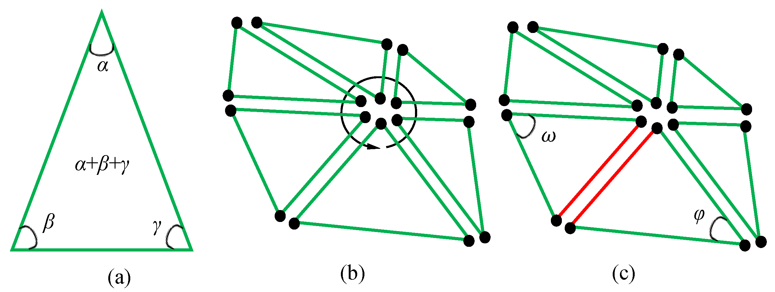
After mesh partitioning, the 3D model can be separated into several disk-type mesh groups. This series of mesh groups is flattened onto the 2D domain based on an angle-preserving and conformal mesh parameterization. The main idea of this parameterization method is to make the difference between angles in the 3D and 2D domains as small as possible. Several topological constraints are also applied during the optimization of the angles to ensure the topological correctness on the 2D domain. The proposed angle-based flattening method sets three kinds of mesh-topology constraints, namely, triangle, vertex and wheel consistencies, as shown in Figure 3a–c. This series of topological constraints can be formulated as the following objective function in a linear system:
where n is the number of meshes; εi is the error of the angle on the ith mesh; α, β, and γ are the angles on each mesh; θd is the angle around the inner vertex; d is the number of angles around the inner vertex; and φ and ω are the angles on two adjacent meshes, respectively, corresponding to the common edge. Equation (3) is essentially Ax = b, where the errors εi, i = 1…n × 3 can be minimized. The optimized angles on the 2D domain can then be obtained by adding the errors and the original angles together.
The new vertices on the 2D domain must be calculated in accordance with the optimized angles. Let three vertices of a triangle be e1, e2 and e3, and the corresponding angles be α1, α2, and α3, respectively. The calculation of the new vertices on the 2D domain uses the following least-squares approximation:
where R is a rotation matrix with angle α1, and j is the jth iteration. Assume that the two vertices e1 and e2 of a triangle are known. Equation (4) employs the known vertices e1 and e2 to optimize the unknown vertex e3, where Qobj is the objective function for the optimization. For all 2D meshes, if the first two vertices on a mesh can be determined, the remaining vertices can be evaluated by using the least-squares approximation [11], which is formulated as a set of linear equations. The topology of all vertices on the UV domain can be maintained correctly.
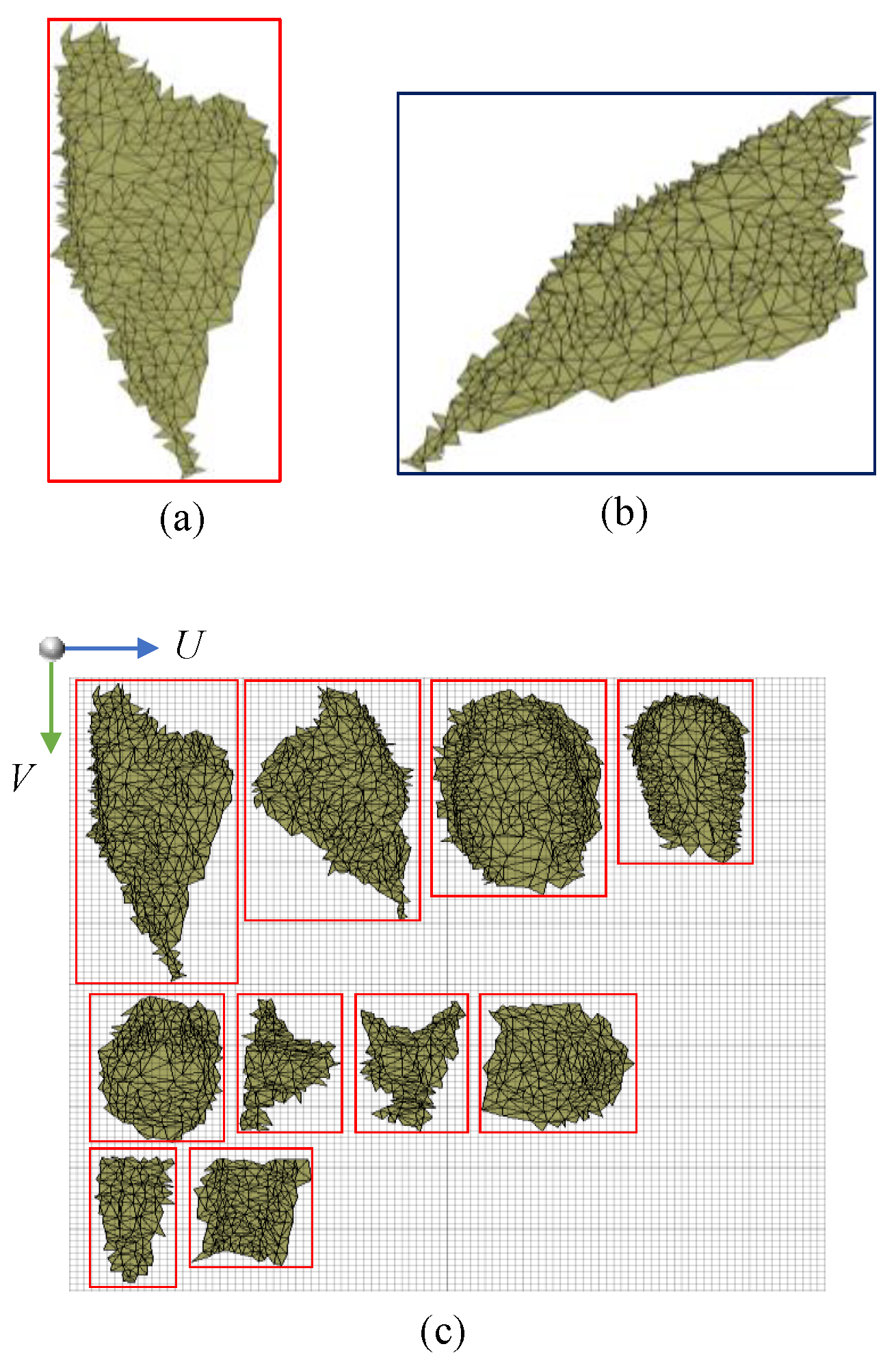
The parameterized mesh islands are all independent. This series of mesh islands needs to be packed together onto the UV map. The UV map is essentially a kind of image that records all 2D meshes and is of the same image size as the texture map. The process of collecting all mesh-islands and converting them into the UV map is called packing. The objective in packing is to let each mesh island occupy as much space as possible, thereby maintaining the resolution of the texture as close to that of the 2D images as possible. Therefore, we consider how to efficiently arrange the mesh islands on the UV map. First, an oriented boundary box (OBB) method [41] is employed to construct a best-fit boundary box for each mesh island, as shown in Figure 4a. Using the OBB method to arrange the islands ensures that less space on the UV map is wasted compared to when using the axis aligned bounding box (AABB) method shown in Figure 4b. Next, the mesh islands are arranged together according to their OBB lengths on the UV map, as shown in Figure 4c.
4.3. Texture Transferring
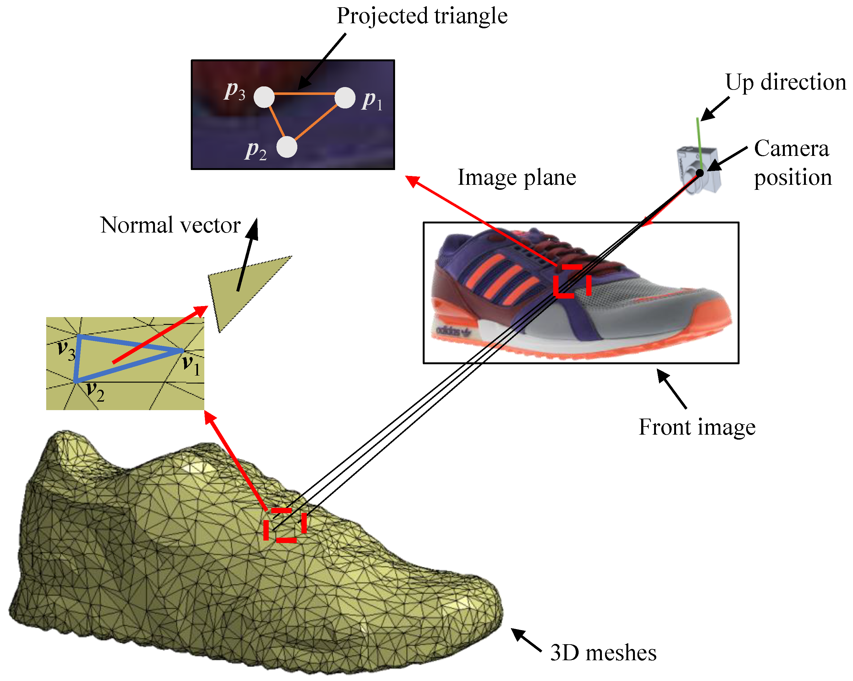
Texture transferring is essentially a process which yields a texture map by filling in each pixel on and inside the mesh islands on the UV map with a color extracted from the object images. The following sentences describe the basic idea of this algorithm (see Figure 5). For each 3D mesh, we allocate the most appropriate object image (called front image hereafter) and extract a triangular range of pixels and color information for this mesh. We can also find a triangular range of pixels on the UV map for the same mesh. However, two pixel ranges might not be the same. Therefore, we perform a transformation for pixel mapping between these two domains. The texture transferring algorithm has three main steps: grouping the 3D meshes, extracting the pixels from object images, and placing the pixels onto the UV map. A detailed description for each step is given below.
4.3.1. Grouping the 3D Meshes
The purpose of this step is to allocate each mesh to a front image and put all meshes that use the same front image in a group. Each mesh can be projected onto several candidate images. The candidate image that yields the largest projected area and hence the highest texture resolution is chosen as the front image. Ideally, all object images could be regarded as the candidate images and selected by all meshes. However, erroneous texture mapping might occur owing to insufficient inaccuracy of the 3D model, as well as camera parameters. A seam line is a photo-inconsistent phenomenon that often occurs at the transition of two different image sources. As the number of candidate images increases, so does the possibility of seam lines. Therefore, to reduce the occurrence of seam lines, we only select some object images as the candidate images and perform mesh grouping.
The algorithm of grouping is as follows. A series of pieces of camera information corresponding to the object images and the 3D meshes are the input. One of the important parameters is the looking vector, which represents the camera viewing direction and is perpendicular to the image plane. In addition, each of the meshes has its own surface normal. The grouping criterion is based on the angle between the looking vector of an image and the surface normal of a mesh. The front image of a mesh is defined as the image with the minimum angle among a set of candidate images. It can yield the largest projected area when projecting the mesh onto the front image. All meshes that use the same front image can thus be grouped.
Visibility should be considered when grouping meshes. The following two criteria are checked to detect the visibility of a mesh. First, the angle between an image and a mesh must be less than 90°. This criterion is employed to ensure that the image faces the front side of the mesh. Second, this mesh cannot be obstructed by other meshes that use the same front image. An obstruction check in terms of the above two criteria could be developed by comparing each mesh with all other meshes. However, it would require substantial computational time. A cell subdivision algorithm [42] is employed to check the possibility of mesh obstruction, which can save the computational time efficiently. The visibility check can prevent the occurrence of mesh obstruction for all meshes on the same group. When the visibility problem occurs on an image, the front image can be selected from one of its two neighboring images.
After these processes, the meshes are grouped. The existence of isolated meshes may result in additional seam lines. An isolated mesh is a small mesh island, which has a front image different to its surrounding meshes. As the boundary of the mesh island represents two different image sources, seam lines easily occur around the boundary of the mesh island. Therefore, when a mesh island is detected, its image source is changed to that of its surrounding meshes. Figure 6 depicts the grouping result of an example using six candidate images.
4.3.2. Extraction of Pixels from the Object Images
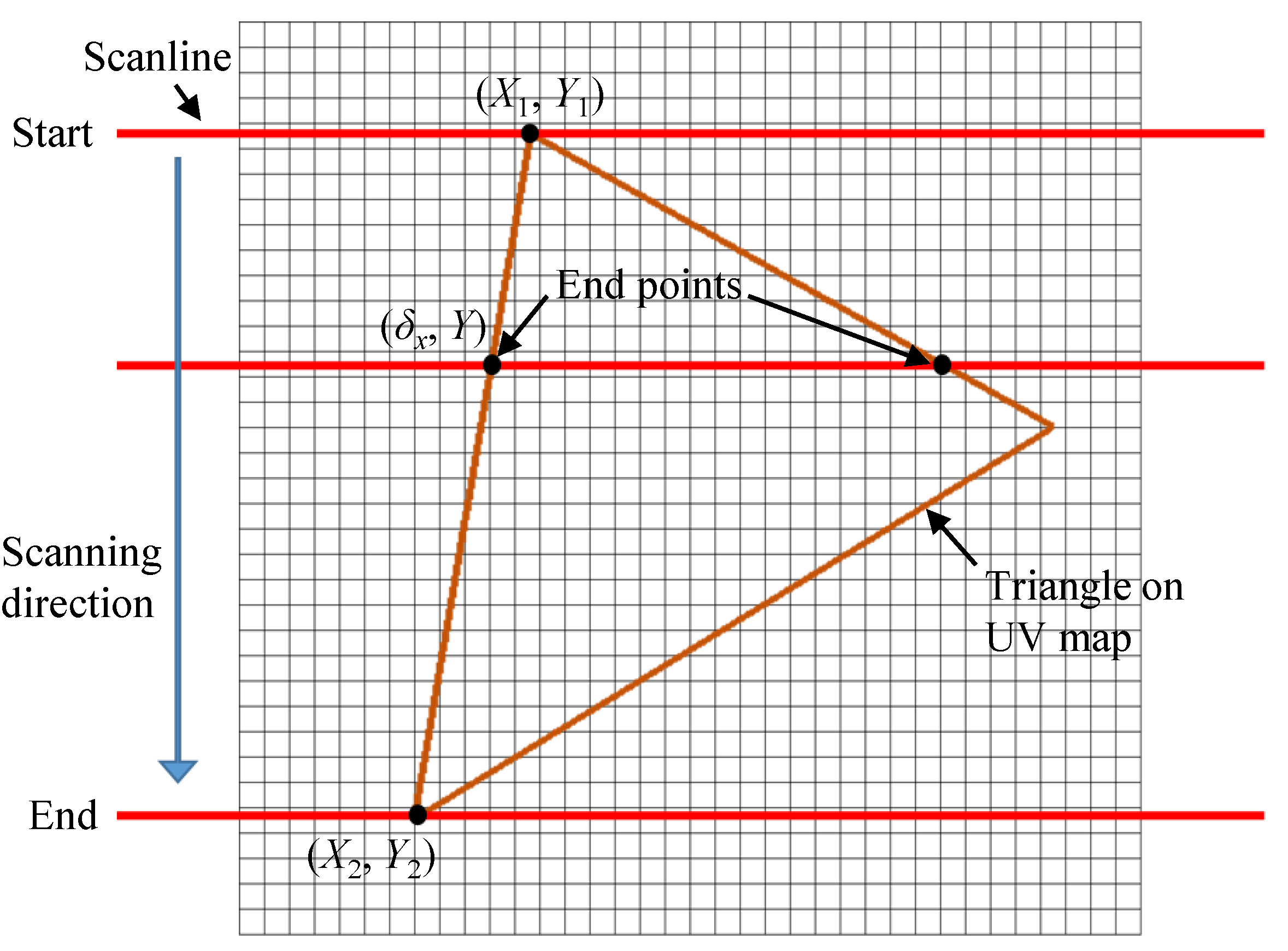
The purpose of this step is to extract pixels from the front image with respect to a 3D mesh. A prospective projection is performed to project 3D meshes back to the image domain. As Figure 5 depicts, the triangle Δp1p2p3 denotes the projection of a 3D mesh Δv1v2v3 onto the image domain. All pixels and color information on and inside this triangle represent the corresponding texture for the 3D mesh. The extraction of a pixel inside a triangle is explained below. The image is made up of pixels in a grid plane containing horizontal and vertical lines, which gives each pixel a unique coordinate. A scanline method is implemented to compute all pixels inside a triangle. The scanline shown in Figure 7 intersects two triangle edges, which yields the two endpoints of the line segment inside the triangle. All pixels on this line segment can then be evaluated in sequence. An endpoint of the line segment can be evaluated by using the following equation:
where (X1, Y1) and (X2, Y2) denote two vertices of an edge on the triangle, Y is the vertical coordinate value of the current scanline, and δx is the horizontal coordinate value of the endpoint on this edge. Equation (5) is applied twice on the left and right edges, respectively, for each scanline.
4.3.3. Placement of Pixels onto the UV Domain
The final step is the placement of pixels onto the UV map. The pixels with respect to each 2D mesh are evaluated in the previous step. However, as each 2D mesh on the UV domain is different from the projected mesh on the image domain, the pixels on these two-pixel domains do not have a one to one correspondence. Therefore, a transformation algorithm must be employed to map the pixels between these two domains. The proposed algorithm is explained below. The three vertices of a mesh on the image domain are respectively mapped onto the corresponding three vertices on the UV domain by using the following equation:
where X and Y denote the coordinates of a vertex on the image domain, and X′ and Y′ denote the coordinates of the corresponding vertex on the UV domain. The parameters a to f can be evaluated as all three pairs of vertices on the image and UV domains are given. Once a to f corresponding to a triangle are obtained, the colors of all pixels within this triangle can thus be interpolated by using Equations (6) and (7). Therefore, all pixels of different triangles on the UV domain can be filled in with correct colors, which yield the texture map for all 2D meshes.
4.4. Texture Correction and Optimization
The purpose of this study is to generate a high quality texture for a 3D mesh model. Thus, the texture correction and optimization need to be investigated to ensure that the texture quality is similar to that of original 2D images. There are four key issues to study: packing the meshes on the UV domain efficiently, arranging the pixel resolution on the texture map, eliminating the influence of geometric error on the 3D model, and blending the texture at the transition of different images. For the first issue, the main idea has already been described in Section 4.2. The meshes can be packed efficiently on the UV map by applying the OBB method to each mesh island, which can yield a smaller boundary box for each mesh island packed on the UV map as compared with the AABB method. In this way, the overall space required for the OBB method is more compact than that without applying the OBB method. Hence, each 2D mesh can allocate more pixels on the UV map, which is especially useful for small meshes with respect to preserving the texture resolution.
The next issue is arranging the overall resolution of the texture map. An object image only partially covers the texture of an object. However, a texture map must cover the entire object texture. If the texture size of a texture map is the same as that of an object image, the image resolution of the texture map is worse than that of the object image. The texture size of an object image used is 5184 × 3456, whereas the original texture size for a texture map is 4096 × 4096. After a careful comparison of several kinds of image resolution, the texture size of the texture map is expanded to 8192 × 8192, with a texture space four times larger than before. This kind of texture size ensures that the pixel number within a mesh on the texture map is close to that of the same mesh projected onto an object image. The original high-quality image information can therefore be kept on the final texture map.
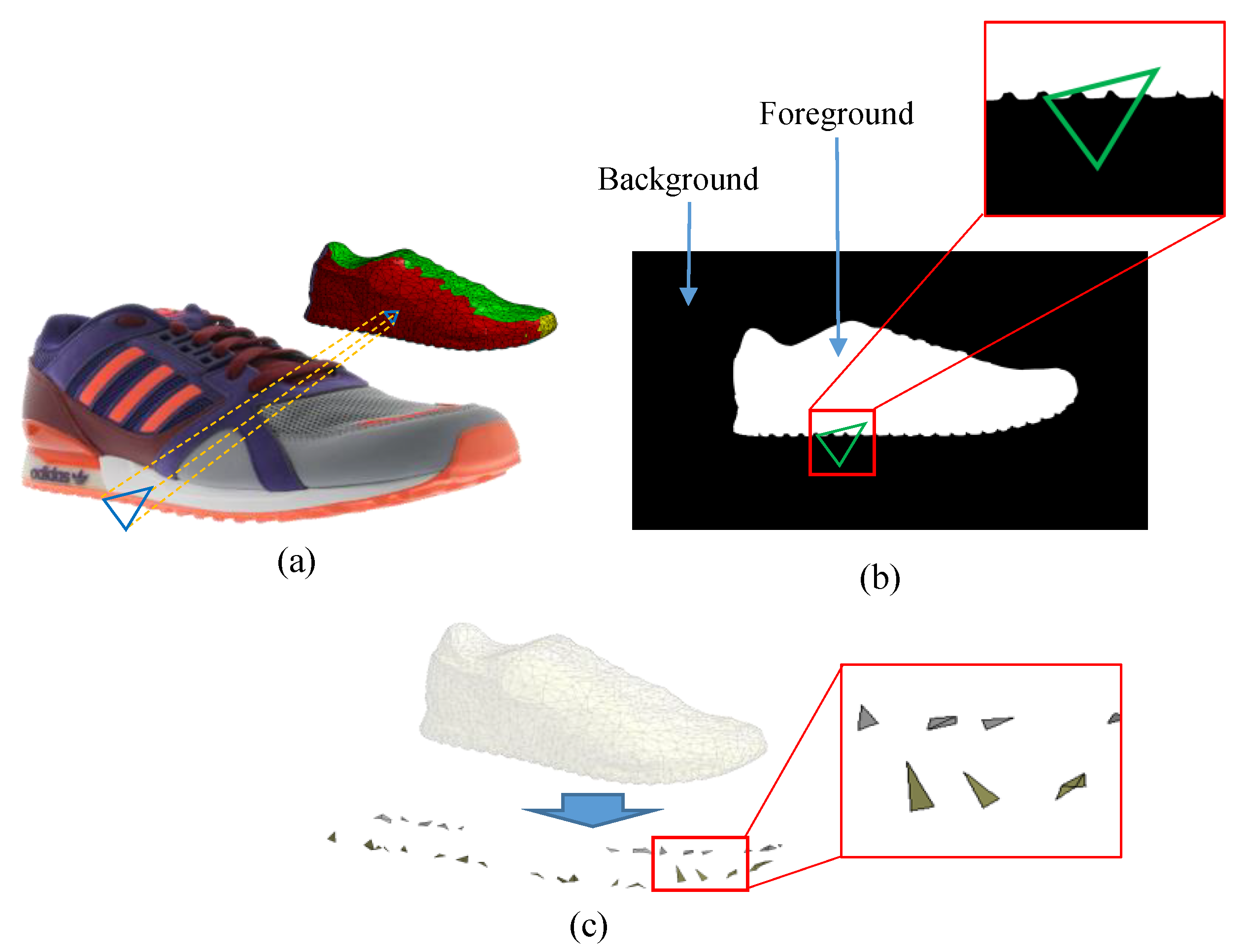
The texture information is extracted from an object image by projecting a 3D mesh onto the corresponding image plane. Normally, a projected mesh is completely inside an image silhouette, and the corresponding range of pixels can be extracted from the projection. However, due to the insufficient accuracy of the 3D model, some of the meshes could be wrongly projected and are partially or completely outside the image silhouette, such as the example in Figure 8a. When a projected mesh is not completely inside the image silhouette, no matching texture can be obtained, and hence the corresponding color is void. To deal with this kind of problem, it is necessary to detect each occurrence of this kind of mesh, and change the front image for each of them. The detection is based on the background removal of object images. First, the object image is converted into a binary image by verifying the foreground and background information. An alpha channel, which records the transparency of each pixel on an object image, is saved and associated with the object image after background removal. This process can be used to verify the foreground and background information of the object image. We convert the object image into black and white in accordance with the data on the alpha channel, such as the example in Figure 8b, where the pixels in white and black denote inside and outside the object, respectively. This additional image is used to check if a projected mesh is outside the image silhouette during the texture transferring process. Since the transferring is scanned pixel by pixel, the black color can be detected and the mesh that covers the black color can be marked for further correction later. Figure 8c depicts the meshes covering pixels of black color, and are marked to individually change their front images. For each of this kind of mesh, the new front image is determined by choosing one of the two neighboring images of the original front image.
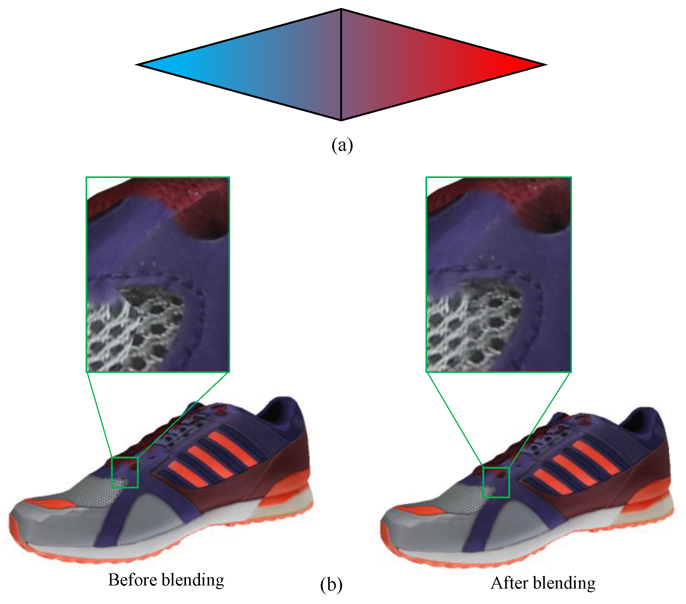
The final optimization is to blend the texture at the transition of different images. The texture is extracted from different front images. However, the texture between different image sources may be inconsistent in color. This difference will cause seam lines on the 3D textured model. The blending between two texture sources can be performed to optimize the color consistency on the model. The boundary meshes should be detected first. The blending is based on the pixel distance to the boundary edge. The equation of color blending is
where P′(i) denotes the blending pixel color of the mesh, Pm (i) denotes the main pixel color of the mesh, Pn (i) denotes the neighboring pixel color of the mesh, Df denotes the farthest pixel of the mesh, and Dc denotes the current pixel of the mesh. Figure 9a depicts the blending of two pixel colors on two neighboring meshes. A linear variation on the weight for blending is applied so that when the distance of the pixel is close to the boundary edge, the weight is larger; whereas, when the distance of the pixel is further from the boundary edge, the weight decreases linearly. That is, the original color information on each mesh is kept if the pixel is far from the boundary edge. In this way, the seam lines on the model can be eliminated to support the consistency of the 3D textured model. Figure 9b shows one example to illustrate the effect of blending, where the left and right plots indicate the results before and after blending, respectively.
P′(i) = (Pm (i) × Df + Pn (i) × (Df − Dc))/(2 × Df − Dc),
5. Result and Discussion
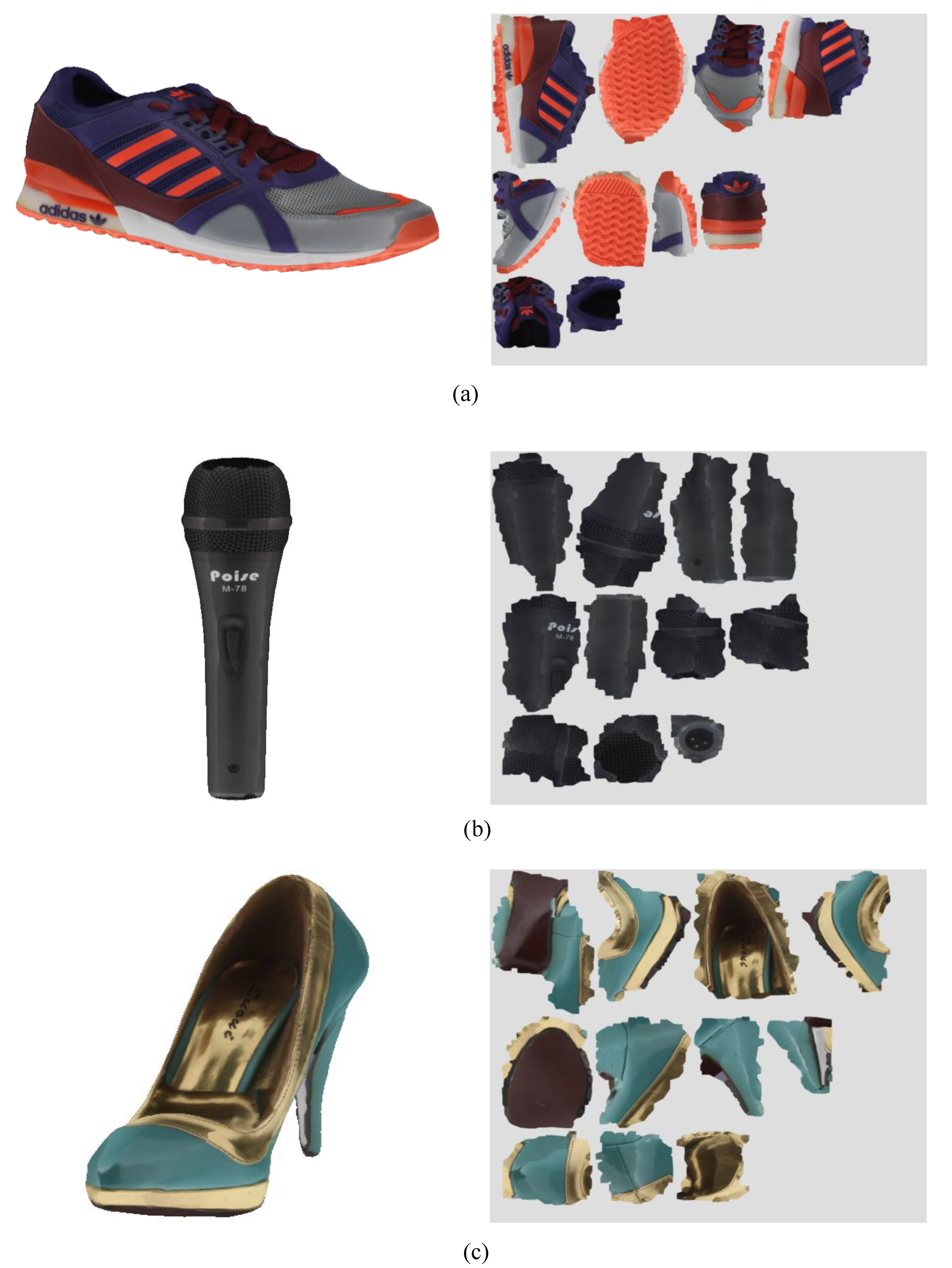
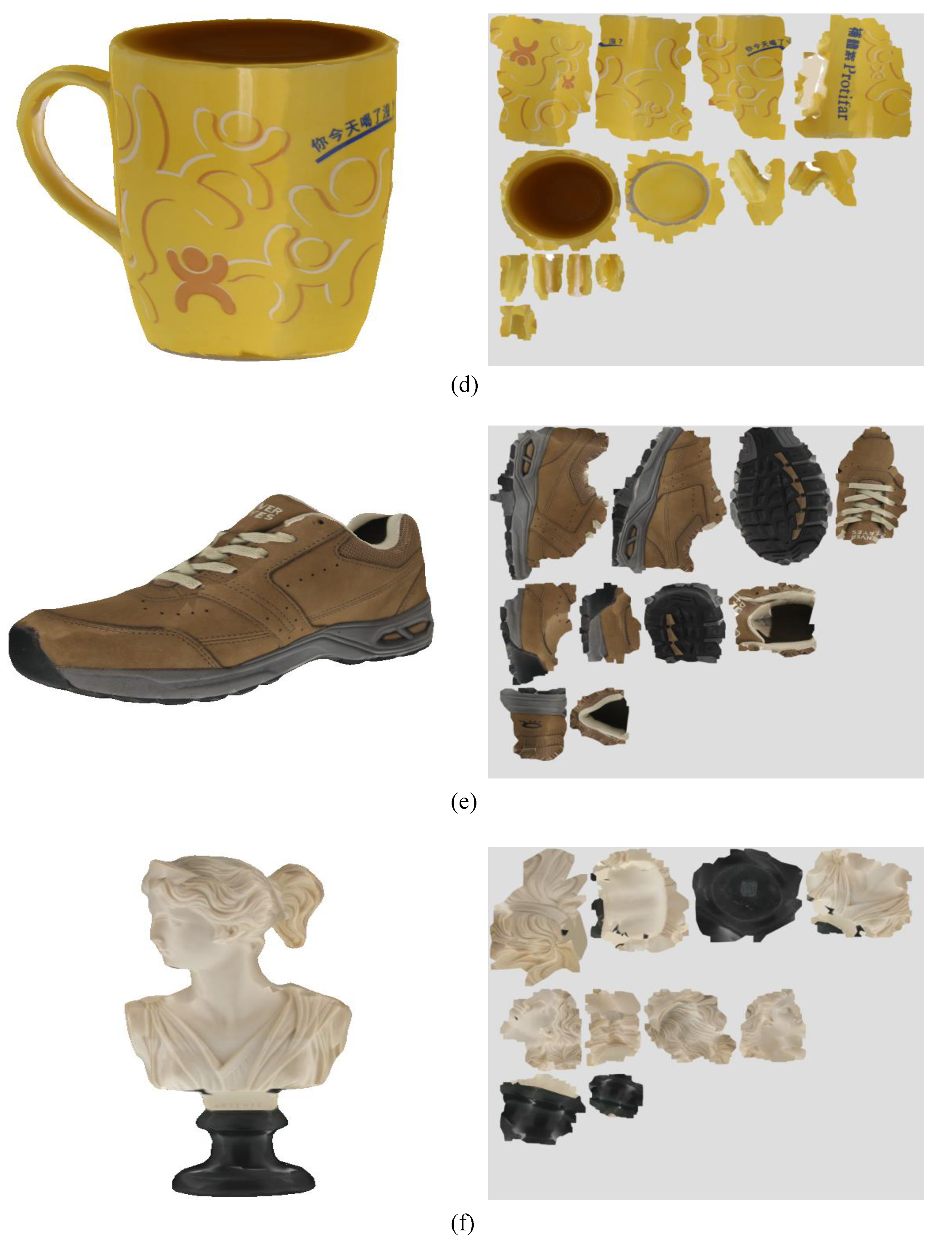
The results of the texture map and 3D textured model for six examples are depicted in Figure 10a–f, where the left and right images in each figure panel denote the 3D textured model and the texture map, respectively. The entire texture mapping process is done automatically, with a 3D model and 16 object images in different views as inputs, and the corresponding texture map as the output. The texture size for all six examples is 8912 × 8912. The proposed process includes the following key procedures: mesh partitioning, mesh parameterization and packing, texture transferring, and correction and optimization of the texture. The initial number of seeds on mesh partitioning is set to 10, and the final number of mesh islands generated for all six examples is 10–13. Each of the results in Figure 10 can be demonstrated as a high-quality 3D textured model by applying the texture correction and optimization during the texture generation process. The results with and without texture correction and optimization are further discussed below.
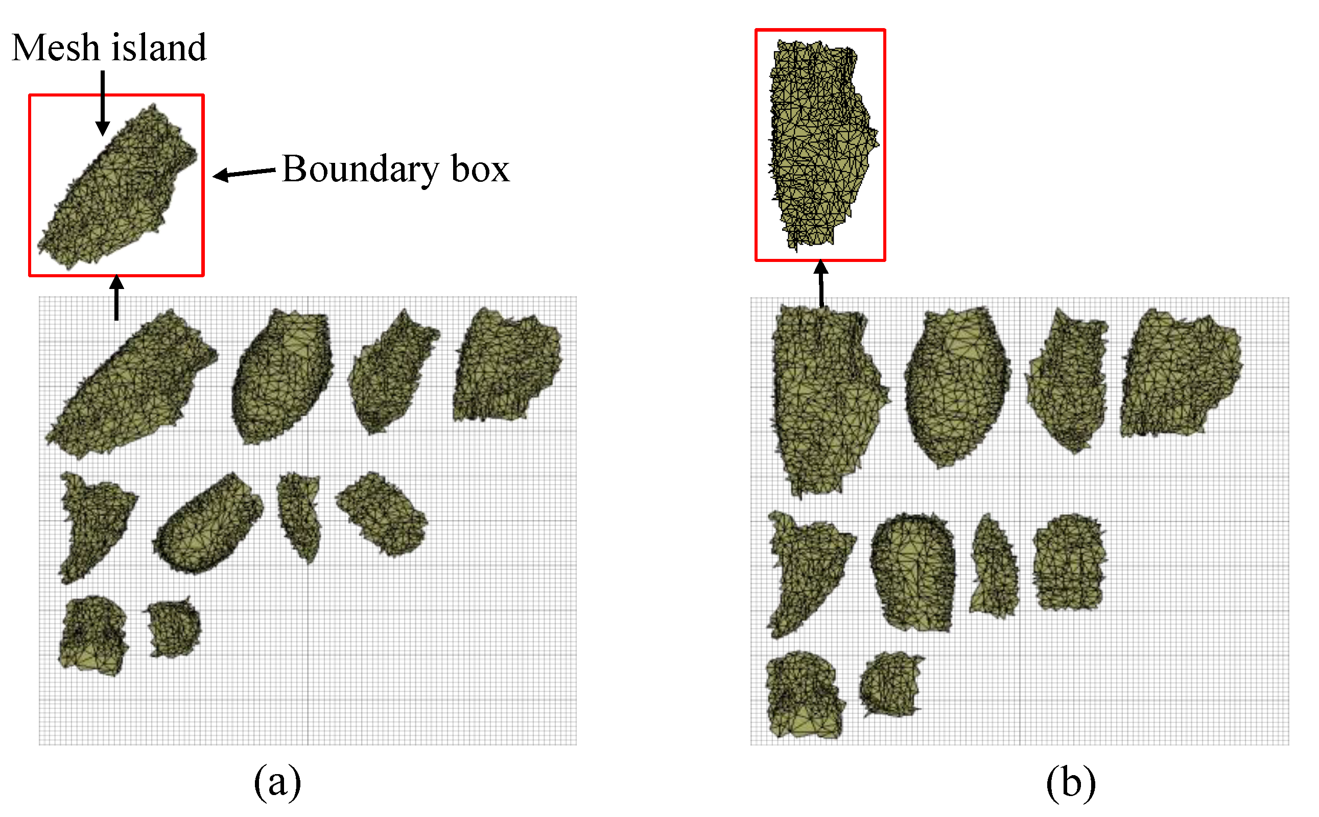
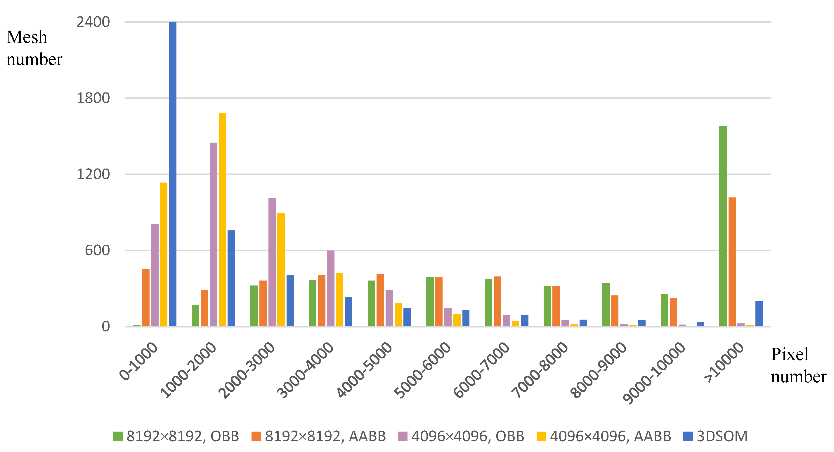
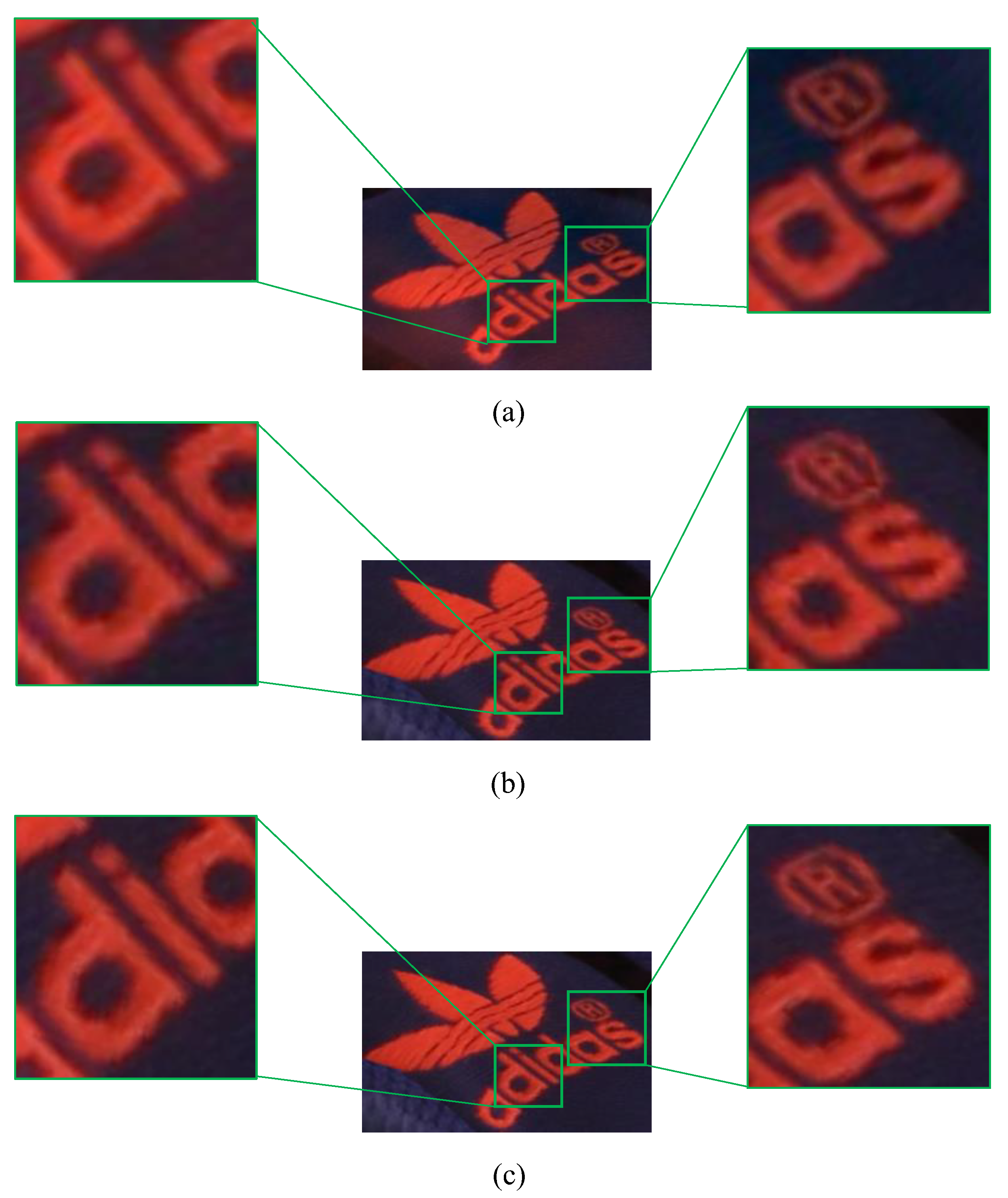
The first optimization process is mesh island packing. When the AABB method is employed (Figure 11a), the bounding box of each mesh island is larger, and the empty space inside each boundary box is also larger. When all these boundary boxes are packed onto a UV map of fixed size, each mesh island is over-compressed and loses the texture resolution that it should have. By contrast, when the OBB method is employed (Figure 11b), each boundary box can best fit its mesh island so that the space that a mesh island occupies is more compact. In addition, the previous resolution of the texture map was 4096 × 4096 pixels. To maintain the resolution 5184 × 3456 of the original image, the larger resolution 8192 × 8192 has been applied to enhance the quality of the final texture. The texture space is four times larger than before. Therefore, each mesh island can be allocated more pixel space when all boundary boxes are packed on the same UV map. Figure 12 depicts the distribution of the mesh number on each range of pixel numbers for the following four cases: 8192 × 8192/OBB, 8192 × 8192/AABB, 4096 × 4096/OBB, 4096 × 4096/AABB and commercial (3DSOM) software [43], where 3DSOM is commercial software. When the number of meshes with fewer pixels is reduced, the texture resolution is closer to that of the original images. It is evident that the texture resolution of the case 8192 × 8192/OBB is the best among the five cases because it has the minimum number of meshes with fewer pixels. In addition, the texture resolution of 3DSOM software is the worst as most of meshes have pixels less than 2000. Therefore, the texture resolution of the proposed method is better than that of 3DSOM software. Figure 13 depicts a local region of the texture for three cases, 3DSOM software, 4096 × 4096/AABB and 8192 × 8192/OBB. The result clearly indicates that the sharpness of the texture in Figure 13c is better than that in Figure 13a,b. The 3DSOM software blends the color with a low-pass filtered image, which will result in a loss on the texture resolution. This result indicates that the proposed method can yield a better texture resolution than 3DSOM software.
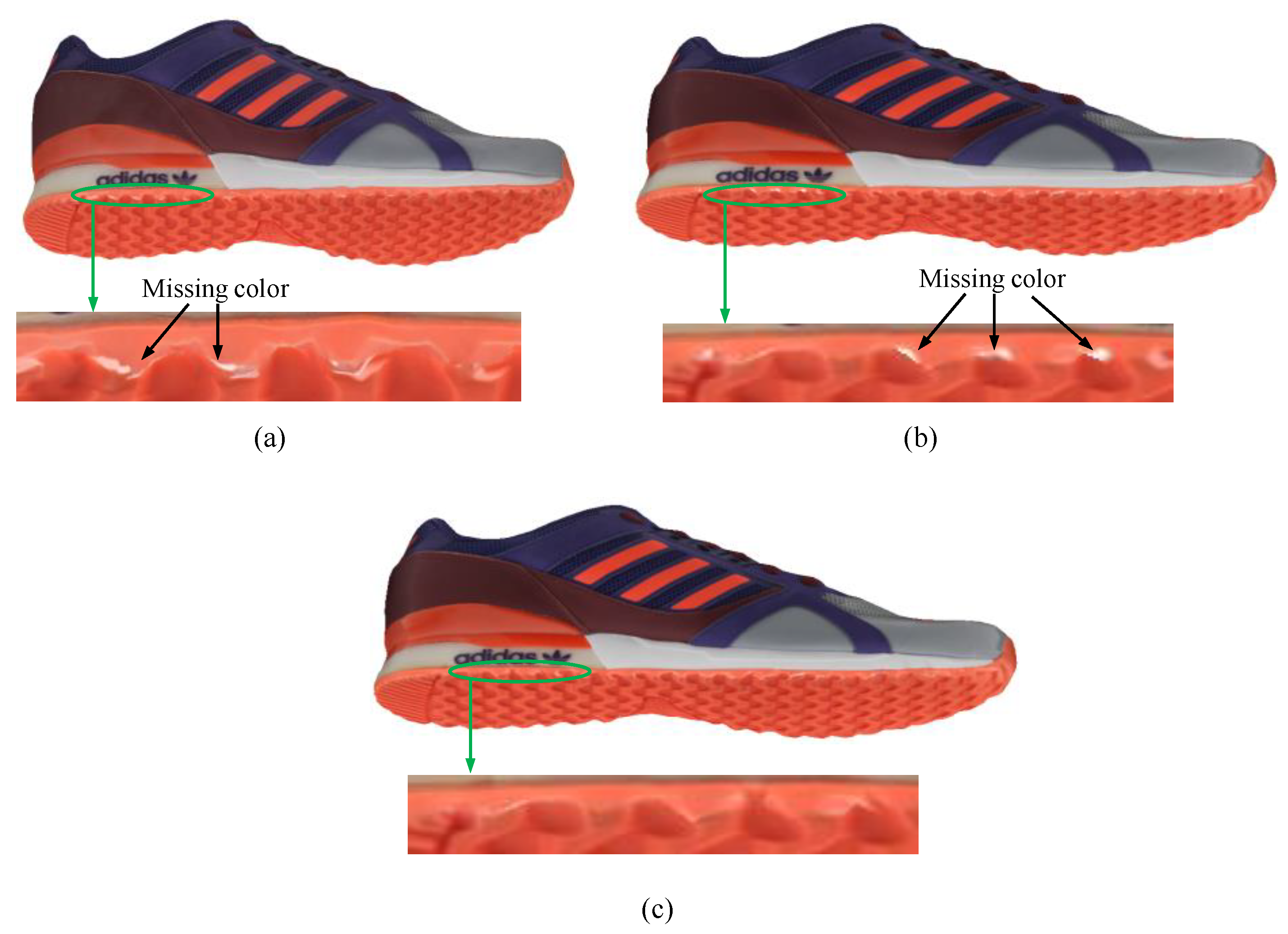
The next optimization process is the elimination of the texture defects caused by the geometric error. The background color of the image might be wrongly extracted for some meshes near the image silhouette, resulting in white spots on the 3D textured model. The incorrect extraction is caused by the meshes that are located outside the image silhouette when they are projected onto the front image. Thus, we wish to eliminate the influence of the error. Figure 14 depicts the comparison of 3DSOM software, the previous result, and the proposed result where, for the previous result, no action was taken to deal with this problem, and for the proposed result, the data on the alpha channel of each object image was employed to detect this problem, and then its front image was replaced where necessary. It is evident that white background spots appear both on the result of 3DSOM software and previous result, they have been eliminated on the proposed result and the color is more consistent on the boundary area. For the e-commerce presentation, the color correctness is increased and the entire model viewing experience is improved.
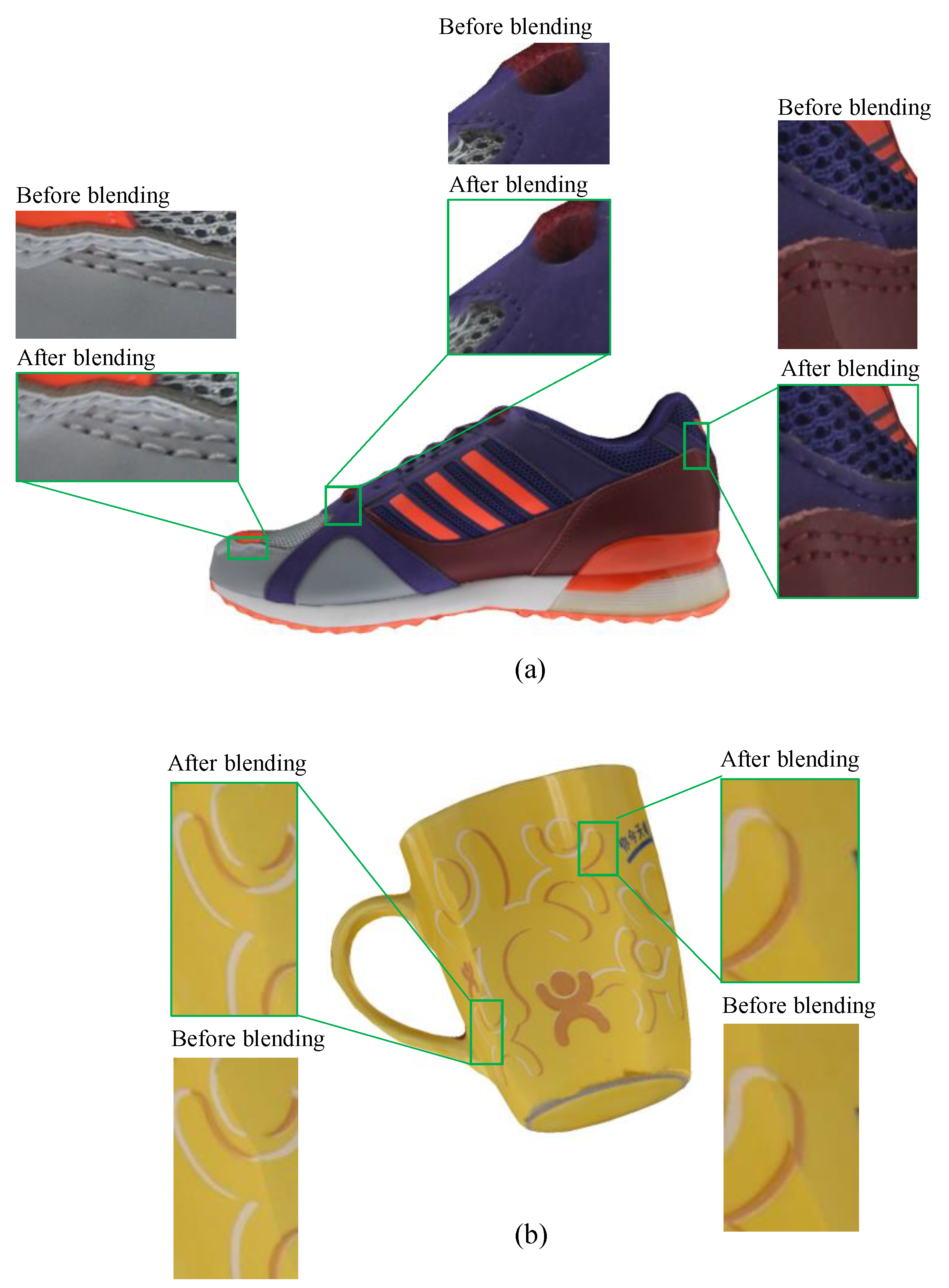
The final optimization process is blending the texture information on the image transition area. The texture information is extracted from different front images. The boundary between two image sources might be inconsistent in color. The results before and after the implementation of the proposed blending algorithm for a shoe and a cup are shown in Figure 15a,b, respectively. The texture quality on the transition area has been improved. The quality of the entire 3D textured model can therefore be improved for the purpose of e-commerce presentation.
6. Conclusions
In this study, we proposed a texture mapping technique that incorporates mesh partitioning, mesh parameterization and packing, texture transferring, and texture correction and optimization. The proposed mesh partition minimizes the growing cost to find the optimized mesh group. The mesh parameterization was based on an angle-based flattening to yield the optimized angles for 2D meshes, and a least-squares approximation to obtain all vertices. The texture transferring was implemented by projecting 3D meshes onto the image domain, and then extracting the pixels to map onto the UV map. However, to maintain the original quality of the texture information, a correction and optimization process was proposed. The OBB method was applied to allocate the UV map space more efficiently in the packing stage. The resolution of the texture map was increased to sufficiently include the original extracted pixels. Additional images were also employed to correct the error extraction of the background color by applying the alpha channel onto the object image. Finally, a blending process was proposed to minimize the transition error caused by different image sources. A high-quality 3D textured model can be obtained by applying this series of processes for presentations in e-commerce. However, the photo consistency of the 3D textured model is still not as good as that of 2D images. The color information from different image sources for the same point may differ slightly. This error is caused by the inaccuracy of 3D vertices and the calibration error; it can affect the projection accuracy of the vertices onto different texture sources. To further improve the quality of the 3D textured model, the photo inconsistency problem should be studied further.
Author Contributions
Conceptualization, J.-Y.L., T.-C.W., W.P., D.W.W., C.-Y.L. and J.-Y.L.; methodology, J.-Y.L. and T.-C.W.; writing—original draft preparation, J.-Y.L. and T.-C.W.; writing—review and editing, J.-Y.L. and T.-C.W.
Funding
This research received no external funding.
Conflicts of Interest
The authors declare no conflicts of interest.
References
- Ortery. Available online: https://www.ortery.com/ (accessed on 1 October 2018).
- Kutulakos, V.; Seitz, S. A theory of shape by space carving. Int. J. Comput. Vis. 2000, 38, 199–218. [Google Scholar] [CrossRef]
- Sinha, S.; Pollefeys, M. Multi-view reconstruction using photo-consistency and exact silhouette constraints: A maximum flow formulation. In Proceedings of the Tenth IEEE International Conference on Computer Vision, Washington, DC, USA, 17–21 October 2005; Volume 1, pp. 349–356. [Google Scholar] [CrossRef]
- Lazebnik, S.; Furukawa, S.; Ponce, J. Projective visual hulls. Int. J. Comput. Vis. 2007, 74, 137–165. [Google Scholar] [CrossRef]
- Mulayim, A.Y.; Yilmaz, U.; Atalay, V. Silhouette-based 3D model reconstruction from multiple images. IEEE Trans. Syst. Man Cybern. Part B Cybern. 2003, 34, 582–591. [Google Scholar] [CrossRef] [PubMed]
- Franco, J.S.; Boyer, E. Exact polyhedral visual hulls. In Proceedings of the British Machine Vision Conference, Norwich, UK, 9–11 September 2003; Volume 1, pp. 329–338. [Google Scholar] [CrossRef]
- Yous, S.; Laga, H.; Kidode, M.; Chihara, K. Gpu-based shape from silhouettes. In Proceedings of the 5th International Conference on Computer Graphics and Interactive Techniques in Australia and Southeast Asia ACM, Perth, Australia, 1–4 December 2007; pp. 71–77. [Google Scholar] [CrossRef]
- Phothong, W.; Wu, T.C.; Lai, J.Y.; Yu, J.Y.; Wang, D.W.; Liao, C.Y. Quality improvement of 3D models reconstructed from silhouettes of multiple images. In Proceedings of the CAD’17, Okayama, Japan, 10–12 August 2017. [Google Scholar] [CrossRef]
- Shamir, A. A survey on mesh segmentation techniques. In Computer Graphics Forum; Blackwell Publishing: Oxford, UK, 2008; Volume 27, pp. 1539–1556. [Google Scholar] [CrossRef]
- Sander, P.; Snyder, J.; Gortler, S.; Hoppe, H. Texture mapping progressive meshes. In Proceedings of the 28th Annual Conference on Computer Graphics and Interactive Techniques, Los Angeles, CA, USA, 12–17 August 2001; pp. 409–416. [Google Scholar] [CrossRef]
- Lévy, B.; Petitjean, S.; Ray, N.; Maillot, J. Least squares conformal maps for automatic texture atlas generation. In Proceedings of the 29th Annual Conference on Computer Graphics and Interactive Techniques, San Antonio, TX, USA, 23–26 July 2002; Volume 21, pp. 362–371. [Google Scholar] [CrossRef]
- Sander, P.; Wood, Z.; Gortler, S.; Snyder, J.; Hoppe, H. Multi-chart geometry images. In Proceedings of the 2003 Eurographics/ACM SIGGRAPH Symposium on Geometry Processing, Aachen, Germany, 23–25 June 2003; pp. 146–155. [Google Scholar] [CrossRef]
- Mangan, A.P.; Whitaker, R.T. Surface segmentation using morphological watersheds. In Proceedings of the IEEE Visualization, 18–23 October 1998. [Google Scholar]
- Mangan, A.P.; Whitaker, R.T. Partitioning 3D surface meshes using watershed segmentation. IEEE Trans. Vis. Comput. Graph. 1999, 5, 308–321. [Google Scholar] [CrossRef] [Green Version]
- Lavoué, G.; Dupont, F.; Baskurt, A. A New cad mesh segmentation method, based on curvature tensor analysis. Comput. Aided Des. 2005, 37, 975–987. [Google Scholar] [CrossRef]
- Mortara, M.; Patan’e, G.; Spagnuolo, M.; Falcidieno, B.; Rossignac, J. Blowing bubbles for multi-scale analysis and decomposition of triangle meshes. Algorithmica 2004, 38, 227–248. [Google Scholar] [CrossRef]
- Mortara, M.; Patan’e, G.; Spagnuolo, M.; Falcidieno, B.; Rossignac, J. Plumber: A method for a multi-scale decomposition of 3d shapes into tubular primitives and bodies. In Proceedings of the Ninth ACM Symposium on Solid Modeling and Applications, Genoa, Italy, 9–11 June 2004; pp. 139–158. [Google Scholar] [CrossRef]
- Funkhouser, T.; Kazhdan, M.; Shilane, P.; Min, P.; Kiefer, W.; Tal, A.; Rusinkiewicz, S.; Dobkin, D. Modeling by example. ACM Trans. Graph. 2004, 23, 652–663. [Google Scholar] [CrossRef]
- Sheffer, A. Model simplification for meshing using face clustering. Comput. Aided Des. 2001, 33, 925–934. [Google Scholar] [CrossRef] [Green Version]
- Garland, M.; Willmott, A.; Heckbert, P. Hierarchical face clustering on polygonal surfaces. In Proceedings of the 2001 Symposium on Interactive 3D Graphics, New York, NY, USA, 19–21 March 2001; pp. 49–58. [Google Scholar] [CrossRef]
- Sheffer, A.; Praun, E.; Rose, K. Mesh parameterization methods and their applications. Found. Trends Comput. Graph. Vis. 2006, 2, 105–171. [Google Scholar] [CrossRef]
- Hormann, K.; Lévy, B.; Sheffer, A. Mesh parameterization: Theory and practice. In ACM SIGGRAPH 2007 Courses on–SIGGRAPH 07; ACM: New York, NY, USA, 2007; Volume 1. [Google Scholar] [CrossRef]
- Desbrun, M.; Meyer, M.; Alliez, P. Intrinsic parameterizations of surface meshes. Comput. Graph. Forum 2002, 21, 209–218. [Google Scholar] [CrossRef]
- Sheffer, A.; De Sturler, E. Parameterization of Faceted Surfaces for Meshing using Angle-Based Flattening. Eng. Comput. 2001, 17, 326–337. [Google Scholar] [CrossRef]
- Sheffer, A.; Lévy, B.; Mogilnitsky, M.; Bogomyakov, A. ABF++: Fast and robust angle based flattening. ACM Trans. Graph. 2005, 24, 311–330. [Google Scholar] [CrossRef]
- Zayer, R.; Lévy, B.; Seidel, H.P. Linear angle based parameterization. In Proceedings of the Fifth Eurographics Symposium on Geometry Processing-SGP, Eurographics Association, Barcelona, Spain, 4–6 July 2007; pp. 135–141. [Google Scholar] [CrossRef]
- Tutte, W.T. Convex Representations of Graphs; London Mathematical Society: London, UK, 1960; Volume 3, pp. 304–320. [Google Scholar]
- Tutte, W.T. How to Draw a Graph; London Mathematical Society: London, UK, 1963; Volume 3, pp. 743–767. [Google Scholar]
- Eck, M.; DeRose, T.D.; Duchamp, T.; Hoppe, H.; Lounsbery, M.; Stuetzle, W. Multiresolution analysis of arbitrary meshes. In Proceedings of the 22nd Annual Conference on Computer Graphics and Interactive Techniques, Los Angeles, CA, USA, 6–11 August 1995; pp. 173–182. [Google Scholar] [CrossRef]
- Floater, M.S. Parametrization and smooth approximation of surface triangulations. Comput. Aided Geom. Des. 1997, 14, 231–250. [Google Scholar] [CrossRef]
- Floater, M.S. Mean value coordinates. Comput. Aided Geom. Des. 2003, 20, 19–27. [Google Scholar] [CrossRef]
- Floater, M.S.; Hormann, K.; Kós, G. A general construction of barycentric coordinates over convex polygons. Adv. Comput. Math. 2006, 24, 311–331. [Google Scholar] [CrossRef]
- Zigelman, G.; Kimmel, R.; Kiryati, N. Texture mapping using surface flattening via multidimensional scaling. Vis. Comput. Graph. 2002, 8, 198–207. [Google Scholar] [CrossRef] [Green Version]
- Degener, P.; Jan, M.; Reinhard, K. An Adaptable Surface Parameterization Method. IMR 2003, 3, 201–213. [Google Scholar]
- Niem, W.; Buschmann, R. Automatic Modelling of 3D Natural Objects from Multiple Views. In Image Processing for Broadcast and Video Production; Springer: London, UK, 1995; pp. 181–193. [Google Scholar]
- Genç, S.; Atalay, V. Texture extraction from photographs and rendering with dynamic texture mapping. In Proceedings of the 10th International Conference on Image Analysis and Processing, Venice, Italy, 27–29 September 1999; pp. 1055–1058. [Google Scholar] [CrossRef]
- Baumberg, A. Blending Images for Texturing 3D Models. In Proceedings of the BMVC, Cardiff, UK, 2–5 September 2002; Volume 3, p. 5. [Google Scholar] [CrossRef]
- Efros, A.A.; Freeman, W.T. Image quilting for texture synthesis and transfer. In Proceedings of the 28th Annual Conference on Computer Graphics and Interactive Techniques ACM, Los Angeles, CA, USA, 12–17 August 2001; pp. 341–346. [Google Scholar] [CrossRef]
- Wei, L.Y.; Levoy, M. Fast texture synthesis using tree-structured vector quantization. In Proceedings of the 27th Annual Conference on Computer Graphics and Interactive Techniques ACM, New Orleans, LA, USA, 23–28 July 2000; pp. 479–488. [Google Scholar] [CrossRef]
- Maruya, M. Generating a Texture Map from Object-Surface Texture Data. In Computer Graphics Forum; Blackwell Science Ltd.: Edinburgh, UK, 1995; Volume 14, pp. 397–405. [Google Scholar]
- Gottschalk, S.; Lin, M.C.; Manocha, D. OBBTree: A hierarchical structure for rapid interference detection. In Proceedings of the 23rd annual conference on Computer graphics and interactive techniques ACM, New Orleans, LA, USA, 4–9 August 1996; pp. 171–180. [Google Scholar] [CrossRef]
- Lai, J.Y.; Shu, S.H.; Huang, Y.C. A cell subdivision strategy for r-nearest neighbors computation. J. Chin. Inst. Eng. 2006, 29, 953–965. [Google Scholar] [CrossRef]
- 3DSOM Software. Available online: https://www.3dsom.com/ (accessed on 1 October 2018).
Figure 1.
Overall flowchart of the proposed texture mapping method: (a) input data, (b) mesh partitioning, (c) mesh parameterization and packing, (d) texture transferring, (e) correction and optimization, and (f) output object file.
Figure 1.
Overall flowchart of the proposed texture mapping method: (a) input data, (b) mesh partitioning, (c) mesh parameterization and packing, (d) texture transferring, (e) correction and optimization, and (f) output object file.

Figure 2.
Flowchart of mesh partitioning.

Figure 3.
Three kinds of mesh-topology constraints in mesh parameterization: (a) triangle consistency, (b) vertex consistency, and (c) wheel consistency.
Figure 3.
Three kinds of mesh-topology constraints in mesh parameterization: (a) triangle consistency, (b) vertex consistency, and (c) wheel consistency.

Figure 4.
Mesh-islands packing: (a) the oriented boundary box (OBB) method to determine the boundary box, (b) the axis aligned bounding box (AABB) method to determine the boundary box, and (c) packing of all mesh-islands.
Figure 4.
Mesh-islands packing: (a) the oriented boundary box (OBB) method to determine the boundary box, (b) the axis aligned bounding box (AABB) method to determine the boundary box, and (c) packing of all mesh-islands.

Figure 5.
Texture transferring.

Figure 6.
The grouping result of a shoe example using six candidate images.

Figure 7.
A scanline method to evaluate all pixels inside a triangle.

Figure 8.
Detection and removal of meshes with missing color: (a) the projected mesh outside the image silhouette, (b) the image converted into foreground (white) and background (black) in accordance with the alpha channel, and (c) meshes detected outside the image silhouette.
Figure 8.
Detection and removal of meshes with missing color: (a) the projected mesh outside the image silhouette, (b) the image converted into foreground (white) and background (black) in accordance with the alpha channel, and (c) meshes detected outside the image silhouette.

Figure 9.
Texture blending at the transition of different images: (a) the blending of two neighboring meshes, and (b) a shoe example before and after blending.
Figure 9.
Texture blending at the transition of different images: (a) the blending of two neighboring meshes, and (b) a shoe example before and after blending.

Figure 10.
The results of the texture map and 3D textured model for six examples: (a) shoe 1, (b) microphone, (c) shoe 2, (d) cup, (e) shoe 3, and (f) statue.
Figure 10.
The results of the texture map and 3D textured model for six examples: (a) shoe 1, (b) microphone, (c) shoe 2, (d) cup, (e) shoe 3, and (f) statue.


Figure 11.
The results of mesh-island packing for two methods: (a) AABB method and (b) OBB method.

Figure 12.
The bar chart of mesh number vs. pixel number for five cases: 8192 × 8192/OBB, 8192 × 8192/AABB, 4096 × 4096/OBB, 4096 × 4096/AABB and 3DSOM software.
Figure 12.
The bar chart of mesh number vs. pixel number for five cases: 8192 × 8192/OBB, 8192 × 8192/AABB, 4096 × 4096/OBB, 4096 × 4096/AABB and 3DSOM software.

Figure 13.
The comparison of texture quality for three cases: (a) 3DSOM software, (b) 4096 × 4096/AABB and (c) 8192 × 8192/OBB.
Figure 13.
The comparison of texture quality for three cases: (a) 3DSOM software, (b) 4096 × 4096/AABB and (c) 8192 × 8192/OBB.

Figure 14.
Implementation of the proposed algorithm to remove missing colors: (a) 3DSOM software (b) before and (c) after.
Figure 14.
Implementation of the proposed algorithm to remove missing colors: (a) 3DSOM software (b) before and (c) after.

Figure 15.
Results before and after the implementation of the proposed blending algorithm: (a) shoe and (b) cup.
Figure 15.
Results before and after the implementation of the proposed blending algorithm: (a) shoe and (b) cup.


Table 1.
Time consuming for mesh partitioning.
| Object | Number of Meshes | No. of Initial Seeds | No. of Final Charts | Total Time (s) |
|---|---|---|---|---|
| Shoe 1 | 4500 * | 10 | 10 | 0.246 |
| 10,000 | 10 | 30 | 1.812 | |
| 20,000 | 10 | 66 | 7.075 | |
| 30,000 | 10 | 111 | 18.431 | |
| 40,000 | 10 | 148 | 31.603 | |
| 50,000 | 10 | 202 | 44.574 |
* used in the case study herein.
© 2018 by the authors. Licensee MDPI, Basel, Switzerland. This article is an open access article distributed under the terms and conditions of the Creative Commons Attribution (CC BY) license (http://creativecommons.org/licenses/by/4.0/).
Share and Cite
MDPI and ACS Style
Lai, J.-Y.; Wu, T.-C.; Phothong, W.; Wang, D.W.; Liao, C.-Y.; Lee, J.-Y. A High-Resolution Texture Mapping Technique for 3D Textured Model. Appl. Sci. 2018, 8, 2228. https://0-doi-org.brum.beds.ac.uk/10.3390/app8112228
AMA Style
Lai J-Y, Wu T-C, Phothong W, Wang DW, Liao C-Y, Lee J-Y. A High-Resolution Texture Mapping Technique for 3D Textured Model. Applied Sciences. 2018; 8(11):2228. https://0-doi-org.brum.beds.ac.uk/10.3390/app8112228
Chicago/Turabian StyleLai, Jiing-Yih, Tsung-Chien Wu, Watchama Phothong, Douglas W. Wang, Chao-Yaug Liao, and Ju-Yi Lee. 2018. "A High-Resolution Texture Mapping Technique for 3D Textured Model" Applied Sciences 8, no. 11: 2228. https://0-doi-org.brum.beds.ac.uk/10.3390/app8112228
Note that from the first issue of 2016, this journal uses article numbers instead of page numbers. See further details here.