Frequency-Domain Filtered-x LMS Algorithms for Active Noise Control: A Review and New Insights

Abstract

This paper presents a comprehensive overview of the frequency-domain filtered-x least mean-square (FxLMS) algorithms for active noise control (ANC). The direct use of frequency-domain adaptive filters for ANC results in two kinds of delays, i.e., delay in the signal path and delay in the weight adaptation. The effects of the two kinds of delays on the convergence behavior and stability of the adaptive algorithms are analyzed in this paper. The first delay can violate the so-called causality constraint, which is a major concern for broadband ANC, and the second delay can reduce the upper bound of the step size. The modified filter-x scheme has been employed to remove the delay in the weight adaptation, and several delayless filtering approaches have been presented to remove the delay in the signal path. However, state-of-the-art frequency-domain FxLMS algorithms only remove one kind of delay, and some of these algorithms have a very high peak complexity and hence are impractical for real-time systems. This paper thus proposes a new delayless frequency-domain ANC algorithm that completely removes the two kinds of delays and has a low complexity. The performance advantages and limitations of each algorithm are discussed based on an extensive evaluation, and the complexities are evaluated in terms of both the peak and average complexities.

1. Introduction

Acoustic noise control is essential for reducing the noise level in modern society since noise seriously affects human health [1,2]. Passive noise control, which is based on using reactive devices, e.g., Helmholtz resonators and quarter wavelength resonators, and using resistive materials, e.g., acoustic linings and porous membranes, is very effective for reducing high-frequency noise, but not so effective for low-frequency noise reduction. Active noise control (ANC) based on the principle of superposition is an appealing method for low-frequency noise reduction [3,4,5,6]. In practice, passive noise control and ANC methods are usually combined to provide wideband noise reduction.

In ANC systems, the filtered-x least mean-square (FxLMS) algorithm is widely used to update the weights of the control filter, but the complexity of the FxLMS algorithm increases linearly with the filter length. In certain applications, the control filter is on the order of several thousand. Therefore, the FxLMS and other time-domain algorithms, e.g., the filtered-x affine projection (FxAP) [7,8,9], are too complex, which is prohibitive for real-time systems. The frequency-domain adaptive filter (FDAF) [10,11,12,13,14,15,16,17] has been successfully used in echo cancellation [18,19,20,21], acoustic feedback cancellation [22], and beamforming [23] due to its good convergence behavior and low complexity. In [24,25,26,27], the block LMS (BLMS) was extended to ANC applications and the corresponding frequency-domain implementation was provided. The experiment in [27] used both the periodic and band-limited signals as the reference signals, but the delay problem was not discussed. In [28], a more efficient implementation of BLMS was presented, where the filtering of the reference signal by the secondary path was also implemented using FFT. Meanwhile, the fast Hartley transform (FHT) was adopted to reduce the complexity. The frequency-domain implementation was extended to the multichannel case in [26,29]. The aforementioned algorithms are obtained by applying the FDAF originally used in echo cancellation to the ANC problem. However, the algorithm requirements for echo cancellation and ANC are quite different. Specifically, the direct use of the FDAF for ANC introduces two kinds of delays. First, there is at least one-block delay between the input of the reference signal and the output of the cancelling signal because the FDAF algorithm is implemented on a block-by-block basis. This delay can violate the causality constraint, which is a major concern for broadband ANC [4,30,31]. Second, the delay between the weight adaptation and the observation of the error signal is introduced because of the effect of the secondary path. The behavior of the filtered-x algorithm is similar to that of the delayed-LMS algorithm, which reduces the upper bound of the step size and slows the convergence and reconvergence rate [32]. In addition, the peak complexity of the FDAF algorithms presented in [28] is quite high because the FFT operation should be completed in one sampling interval; therefore, these algorithms are impractical for real-time implementation.

Many approaches have been proposed to reduce the two kinds of delays. The modified filtered-x structure [33,34] was used in the frequency-domain ANC in [35], which makes the adaptive algorithm behave like the standard FDAF and thus removes the delay in the weight adaptation. The partitioned-block FDAF (PBFDAF) algorithm was introduced for ANC to reduce the delay in the signal path [36,37,38,39]. This is achieved by partitioning the whole impulse response into several small sections, but this method does not completely eliminate the input-output delay. Several delayless algorithms were then proposed to totally remove the delay in the signal path. The calculation of the adaptive filter output can be implemented directly using the time-domain convolution and hence the delay in the signal path is removed [40,41,42,43]. However, the complexity of the convolution in the time domain is still high. In [44], a delayless FDAF algorithm originally used in echo cancellation [45] was extended to ANC, but the computational burden at certain sampling periods is rather high. Two computationally efficient FDAF algorithms for ANC were proposed in [46,47] using the delayless approach in [48,49], but the delay in the filter adaptation is not removed.

Although many efforts have been devoted to the frequency-domain FxLMS algorithms, these algorithms are not well compared and analyzed. To fill this gap, this paper presents a comprehensive review of the frequency-domain FxLMS algorithms. Only mono-channel algorithms are considered in this paper, since they can be straightforwardly extended to the multi-channel case. The conventional frequency-domain FxLMS algorithms are reviewed, and then the effects of the two kinds of delays on the overall performance are analyzed. Specifically, it was found that calculating the adaptive filter output and the weight vector update in different ways leads to different convergence performances, which is quite different from system identification problems. The update-first approach is then proposed to improve the stability. Several delayless frequency-domain algorithms for ANC are surveyed, but these algorithms did not remove the delay related to the secondary path. To address this problem, we present a new delayless frequency-domain FxLMS algorithm to completely remove the aforementioned two types of delays and overcome the shortcomings of the state-of-the-art frequency-domain FxLMS algorithms. The complexity of the frequency-domain approaches in terms of both peak and average multiplications per sample are evaluated. Simulations are carried out to evaluate the convergence performance and stability of the frequency-domain FxLMS algorithms.

2. FxLMS Algorithm

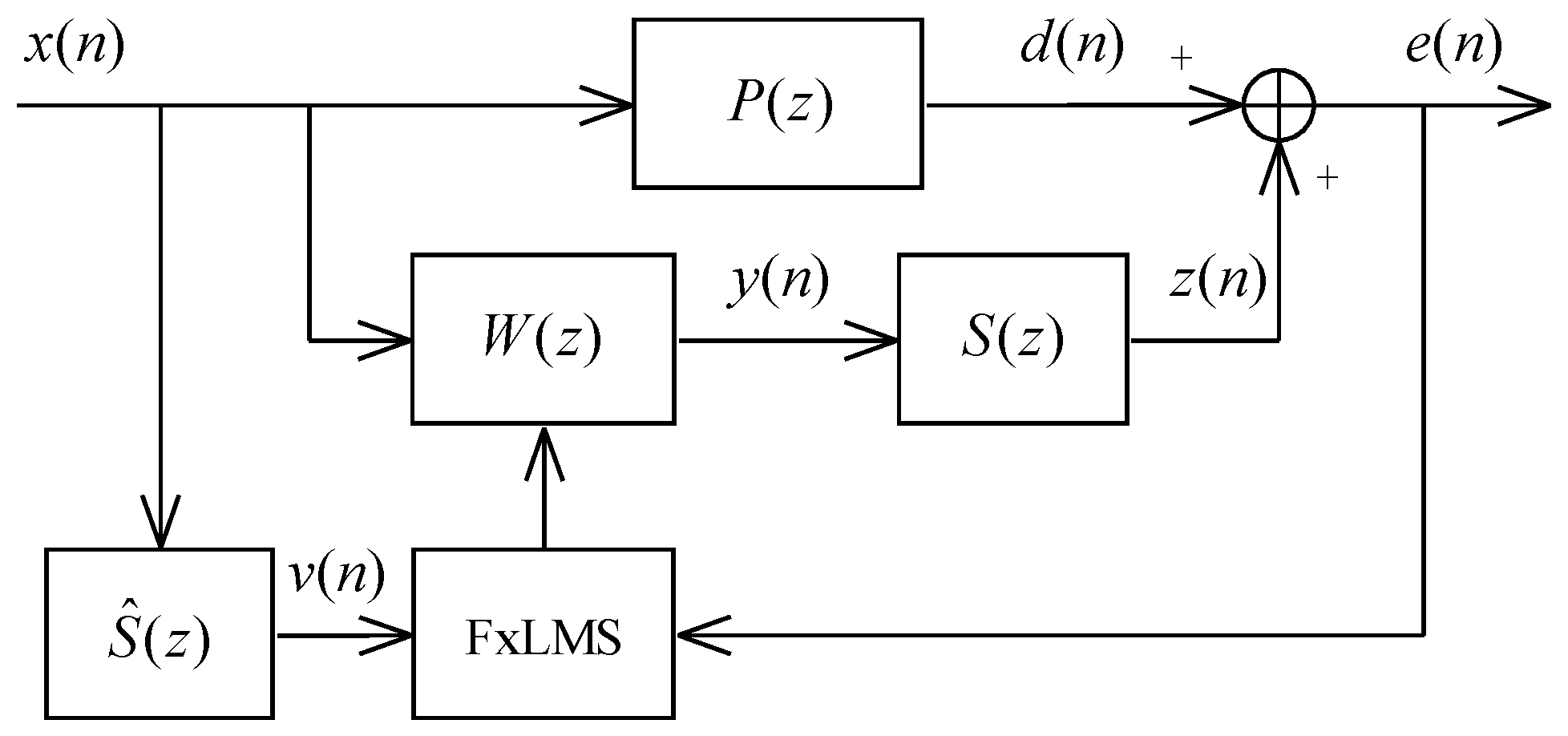
The diagram of the FxLMS algorithm is presented in Figure 1, where $P\left(z\right)$ is the primary path and $S\left(z\right)$ is the secondary path. We define the weight vector of the control filter at the time index n as $\mathbf{w}\left(n\right)={[w_0\left(n\right),w_1\left(n\right),\cdots ,w_{N_{\mathrm{w}}-1}\left(n\right)]}^T$ with a length of $N_{\mathrm{w}}$. The reference signal $x\left(n\right)$ is picked up by a reference microphone and then filtered by the adaptive filter to generate the cancelling signal $y\left(n\right)$ driven by a secondary loudspeaker

$$y\left(n\right)={\mathbf{x}}^T\left(n\right)\mathbf{w}\left(n\right)$$

(1)

where $\mathbf{x}\left(n\right)={[x\left(n\right),x(n-1),\cdots ,x(n-N_{\mathrm{w}}+1)]}^T$ is the reference signal vector. The cancelling signal $y\left(n\right)$ is then filtered by the secondary path $S\left(z\right)$ to obtain the control signal $z\left(n\right)$ at the location of the error microphone

$$z\left(n\right)={\overline{\mathbf{y}}}^T\left(n\right)\mathbf{s}$$

(2)

where $\overline{\mathbf{y}}\left(n\right)={[y\left(n\right),y(n-1),\cdots ,y(n-N_{\mathrm{s}}+1)]}^T$, and $\mathbf{s}={[s_0,s_1,\cdots ,s_{N_{\mathrm{s}}-1}]}^T$ is the weight vector of the secondary path with a length of $N_{\mathrm{s}}$. The residual error signal picked up by the error microphone is

$$e\left(n\right)=d\left(n\right)+z\left(n\right),$$

(3)

where $d\left(n\right)$ is the disturbance signal at the error microphone.

The FxLMS algorithm is commonly used to update the weight vector [3,4]

$$\mathbf{w}(n+1)=\mathbf{w}\left(n\right)-\mu \mathbf{v}\left(n\right)e\left(n\right)$$

(4)

where $\mu$ is the step size, and $\mathbf{v}\left(n\right)={[v\left(n\right),v(n-1),\cdots ,v(n-N_{\mathrm{w}}+1)]}^T$ the filtered reference signal vector, where the filtered reference signal $v\left(n\right)$ is given by

$$v\left(n\right)={\mathbf{x}}_s^T\left(n\right)\widehat{\mathbf{s}}$$

(5)

where ${\mathbf{x}}_s\left(n\right)={[x\left(n\right),x(n-1),\cdots ,x(n-N_{\mathrm{s}}+1)]}^T$, and $\widehat{\mathbf{s}}={[{\widehat{s}}_0,{\widehat{s}}_1,\cdots ,{\widehat{s}}_{N_{\mathrm{s}}-1}]}^T$ is an estimate of the actual weight vector of the secondary path. An accurate estimate of the secondary path is required for the FxLMS to work properly, which can be obtained by an offline- or online-modeling method [4,6].

The FxLMS algorithm requires $2N_{\mathrm{w}}+N_{\mathrm{s}}$ multiplications. In certain scenarios, the length of the weight vector may reach several thousand taps. Thus, the computational complexity is a major concern for real-time systems.

3. Conventional Frequency-Domain ANC Algorithms

The conventional frequency-domain ANC algorithms in [24,25,26,27,28,37,39] can be understood as direct frequency-domain implementations of the FxLMS algorithm. Since the FDAF algorithm is a special case of PBFDAF, we only present the PBFDAF in this paper. The corresponding method using the conventional filtered-x scheme is referred to as the frequency-domain partitioned block filtered-x LMS (FPBFxLMS) algorithm. The method using the modified filtered-x scheme is referred to as the frequency-domain partitioned block modified filtered-x LMS (FPBMFxLMS) algorithm.

3.1. FPBFxLMS Algorithm

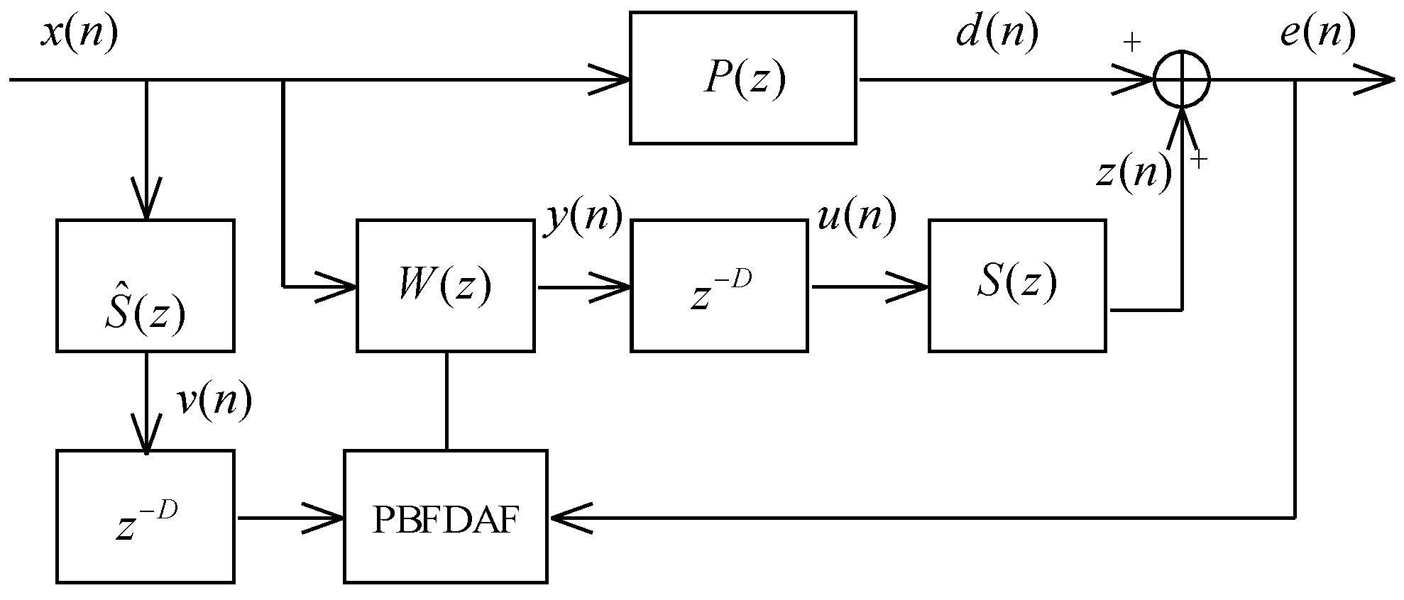
The diagram of the FPBFxLMS algorithm is shown in Figure 2. The linear convolution operations (1) and (5) and the cross-correlation (4) can be implemented using FFTs. The adaptive filter $\mathbf{w}\left(n\right)$ is segmented into $P_{\mathrm{w}}$ partitions as $\mathbf{w}\left(n\right)={[{\mathbf{w}}_0^T\left(n\right),...,{\mathbf{w}}_{P_{\mathrm{w}}-1}^T\left(n\right)]}^T$, where ${\mathbf{w}}_p\left(n\right)={[w_{pL}\left(n\right),...,w_{(p+1)L-1}\left(n\right)]}^T$ is the p-th subfilter with $L=N_{\mathrm{w}}/P_{\mathrm{w}}$ taps. The frequency-domain weight vector of the p-th partition is

$${\mathbf{W}}_p\left(k\right)=\mathbf{F}{[{\mathbf{w}}_p^T\left(k\right),{\mathbf{0}}_{1\times L}]}^T$$

(6)

where k denotes the frame index, ${\mathbf{0}}_{1\times L}$ is a $1\times L$ all-zero vector, and $\mathbf{F}$ is the Fourier transform matrix whose $(p,q)$-th element is $exp(-\mathrm{j}\frac{2\pi pq}{2L})$ with $0\le p\le 2L-1,0\le q\le 2L-1$ and $\mathrm{j}=\sqrt{-1}$. The output of the control filter at the k-th frame is

$$\begin{array}{c}\mathbf{y}\left(k\right)={\left[y(kL-L+1),...,y\left(kL\right)\right]}^T\hfill \\ \begin{array}{cc}& \end{array}={\mathbf{Q}}^{01}{\mathbf{F}}^{-1}\sum _{p=0}^{P_{\mathrm{w}}-1}{\mathbf{X}}_p\left(k\right){\mathbf{W}}_p\left(k\right),\hfill \end{array}$$

(7)

where ${\mathbf{Q}}^{01}=\left[{\mathbf{0}}_L\begin{array}{c}\end{array}{\mathbf{I}}_L\right]$ is the projection matrix (the notations ${\mathbf{0}}_L$ and ${\mathbf{I}}_L$ being the $L\times L$ zeros and identity matrices, respectively), and

$${\mathbf{X}}_p\left(k\right)=diag\left\{\mathbf{F}{\mathbf{x}}_p\left(k\right)\right\}$$

(8)

is the frequency-domain reference matrix with ${\mathbf{x}}_p\left(k\right)={\{x[(k-p-2)L+1],...,x\left[(k-p)L\right]\}}^T$ ($diag\{·\}$ denoting the diagonal matrix).

For the FxLMS algorithm, the output of the control filter is calculated on a sample-by-sample basis and hence there is only one-sample delay for the generation of the cancelling signal. For the frequency-domain implementation in (7), however, a block of the reference signals should be collected before the calculation of $\mathbf{y}\left(k\right)$. There is at least one-block delay even if (7) is completed in one sample period. Thus, the cancelling signal driven by the loudspeaker is a delayed version of $y\left(n\right)$:

$$u\left(n\right)=y(n-D)$$

(9)

where D denotes the delay, which includes both the buffering time and the processing time. In [28,37], the calculation of (7) is completed in one-sample period and hence the total delay $D=L$. In [39], the calculation of (7) is distributed in one block $KL\le n\le KL+L$, and thus the delay is $D=2L$. The advantages and limitations of each implementation method are discussed later.

The impulse response of the secondary path is segmented into $P_{\mathrm{s}}$ partitions as $\widehat{\mathbf{s}}={[{\widehat{\mathbf{s}}}_0^T,{\widehat{\mathbf{s}}}_1^T,...,{\widehat{\mathbf{s}}}_{P_{\mathrm{s}}-1}^T]}^T$, where ${\widehat{\mathbf{s}}}_p={[{\widehat{s}}_{pL},...,{\widehat{s}}_{(p+1)L-1}]}^T$ is the p-th subfilter with $L=N_{\mathrm{s}}/P_{\mathrm{s}}$ taps. The Fourier transform of ${\widehat{\mathbf{s}}}_p$ is

$${\widehat{\mathbf{S}}}_p=\mathbf{F}{[{\widehat{\mathbf{s}}}_p^T,{\mathbf{0}}_{1\times L}]}^T.$$

(10)

The linear convolution in (5) can also be implemented using FFT

$$\begin{array}{c}\mathbf{v}\left(k\right)={\left[v(kL-L+1),...,v\left(kL\right)\right]}^T\hfill \\ ={\mathbf{Q}}^{01}{\mathbf{F}}^{-1}\sum _{p=0}^{P_{\mathrm{s}}-1}{\mathbf{X}}_p\left(k\right){\widehat{\mathbf{S}}}_p.\hfill \end{array}$$

(11)

The update equation of the FPBFxLMS algorithm is [10,16,37,39]

$${\mathbf{W}}_p(k+1)={\mathbf{W}}_p\left(k\right)-\mu {\mathbf{G}}^{10}{\mathbf{\Lambda }}^{-1}\left(k\right){\mathbf{V}}_p^H(k-m)\mathbf{E}\left(k\right),$$

(12)

where ${(·)}^H$ denotes the Hermitian operation,

$${\mathbf{G}}^{10}=\mathbf{F}\left[\begin{array}{cc}{\mathbf{I}}_L& {\mathbf{0}}_L\\ {\mathbf{0}}_L& {\mathbf{0}}_L\end{array}\right]{\mathbf{F}}^{-1}$$

(13)

is the windowing matrix that forces the last L time-domain elements to zero,

$$\mathbf{E}\left(k\right)=\mathbf{F}{[{\mathbf{0}}_{1\times L},{\mathbf{e}}^T\left(k\right)]}^T$$

(14)

is the frequency-domain error vector with $\mathbf{e}\left(k\right)={\left[e(kL-L+1),...,e\left(kL\right)\right]}^T$,

$${\mathbf{V}}_p\left(k\right)=diag\left\{\mathbf{F}{\mathbf{v}}_p\left(k\right)\right\}$$

(15)

is the filtered reference signal matrix with ${\mathbf{v}}_p\left(k\right)={\{v[(k-p-2)L+1],...,v\left[(k-p)L\right]\}}^T$, $\mathbf{\Lambda }\left(k\right)$ is the PSD matrix of the filtered reference signal which is used to improve the convergence, and the parameter m is related to the algorithm latency

$$m=\left\{\begin{array}{c}1\begin{array}{c}\end{array}D=L\\ 2\begin{array}{c}\end{array}D=2L\end{array}\right..$$

(16)

The PSD matrix $\mathbf{\Lambda }\left(k\right)$ can be computed recursively [10,16]

$$\mathbf{\Lambda }\left(k\right)=\lambda \mathbf{\Lambda }(k-1)+(1-\lambda ){\mathbf{V}}_0^H\left(k\right){\mathbf{V}}_0\left(k\right)$$

(17)

where $\lambda$ is a smoothing factor, $0<\lambda <1$.

To reduce the complexity while retaining good convergence properties, the constraint in (12) can be added periodically [50,51]. Another way to reduce the complexity of (12) is to use the unconstrained algorithm [13]

$${\mathbf{W}}_p(k+1)={\mathbf{W}}_p\left(k\right)-\mu {\mathbf{\Lambda }}^{-1}\left(k\right){\mathbf{V}}_p^H(k-m)\mathbf{E}\left(k\right).$$

(18)

The unconstrained PBFDAF exhibits a lower complexity than the constrained version, but the constrained version has a better convergence. Thus, we only consider the constrained FDAF.

The frequency-domain FxLMS algorithms with $D=L$ and $D=2L$ are presented in

Table 1. FPBFxLMS I [28,37].

Operation	Complexity
(1) Compute the frequency-domain reference matrix ${\mathbf{X}}_0\left(k\right)$ using (8)	One FFT
(2) Compute the output of the control filter using (7)	One FFT and $4L{P}_{\mathrm{w}}$ multiplications
(3) Compute the filtered reference signal vector $\mathbf{v}\left(k\right)$ using (11)	One FFT and $4L{P}_{\mathrm{s}}$ multiplications
(4) Compute the FFT of ${\mathbf{v}}_0\left(k\right)$ using (15)	One FFT
(5) Update $\mathbf{\Lambda }\left(k\right)$ using (17)	$4L$ multiplications
(6) Compute the FFT of the error signal using (14)	One FFT
(7) Update the weight vector using (12)	$2P_{\mathrm{w}}$ FFTs and $6L{P}_{\mathrm{w}}$ multiplications
(8) Compute the cancelling signal using (9): $u\left(n\right)=y(n-L)$	0

Note: Steps (1)–(7) should be completed between $kL$ and $kL+1$; Average multiplications: $(5+2P_{\mathrm{w}})A/L+10P_{\mathrm{w}}+4P_{\mathrm{s}}$; Peak multiplications: $(5+2P_{\mathrm{w}})A+10L{P}_{\mathrm{w}}+4L{P}_{\mathrm{s}}+4L$.

and

Table 2. FPBFxLMS II [39].

Operation	Complexity
(1) Compute the frequency-domain reference matrix ${\mathbf{X}}_0\left(k\right)$ using (8)	One FFT
(2) Compute the output of the control filter using (7)	One FFT and $4L{P}_{\mathrm{w}}$ multiplications
(3) Compute the filtered reference signal vector $\mathbf{v}\left(k\right)$ using (11)	One FFT and $4L{P}_{\mathrm{s}}$ multiplications
(4) Compute the FFT of ${\mathbf{v}}_0\left(k\right)$ using (15)	One FFT
(5) Update $\mathbf{\Lambda }\left(k\right)$ using (17)	$4L$ multiplications
(6) Compute the FFT of the error signal using (14)	One FFT
(7) Update the weight vector using (12)	$2P_{\mathrm{w}}$ FFTs and $6L{P}_{\mathrm{w}}$ multiplications
(8) Compute the cancelling signal using (9): $u\left(n\right)=y(n-2L)$	0

Note: Steps (1)–(7) should be completed between $kL$ and $kL+L$; Average and peak multiplications: $(5+2P_{\mathrm{w}})A/L+10P_{\mathrm{w}}+4P_{\mathrm{s}}$.

, respectively, where A denotes the number of multiplications of the $2L$-point FFT operation. The differences between the two algorithms are twofold. First, the FPBFxLMS II algorithm has a larger delay, which limits its application in broadband ANC. Second, the complexity of the FPBFxLMS II algorithm is distributed evenly in one frame, while steps (1)–(7) of the FPBFxLMS I algorithm should be completed in one-sample period. Therefore, the peak complexity of the FPBFxLMS I algorithm is rather high. This means that a strong processor should be used, and a large portion of power is wasted due to the unbalanced complexity [46,48,49]. From the perspective of real-time implementation, the FPBFxLMS I algorithm is not practical. A real-time multichannel ANC system using the FPBFxLMS II algorithm was implemented in the Graphics Processing Unit (GPU) in [39], and a comprehensive complexity evaluation was carried out.

3.2. Analysis

In this section, we carry out theoretical analysis on the effects of the two kinds of delays on the adaptive algorithm convergence behaviors. When the FxLMS converges, the optimal solution (which may not be realizable) in the z-domain is [4]

$$W_{\mathrm{opt}}\left(z\right)=\frac{P\left(z\right)}{S\left(z\right)}.$$

(19)

For the FPBFxLMS algorithms, a D-sample delay is introduced to the signal path, and hence the optimal solution becomes

$$W_{\mathrm{opt}}\left(z\right)=\frac{P\left(z\right)}{z^{-D}S\left(z\right)}.$$

(20)

When the FDAF algorithm is applied for echo cancellation, the algorithm delay has no effect on the algorithm convergence. However, this is not the case for broadband ANC because the causality solution of (20) may not exist and the extra delay in the signal path deteriorates the noise reduction performance [30,31]. For the broadband ANC system to work properly, the casualty condition should be satisfied [3]

$${\tau }_{\mathrm{buff}}+{\tau }_{\mathrm{proc}}+{\tau }_{sec}\le {\tau }_{\mathrm{AD}},$$

(21)

where ${\tau }_{sec}$ includes the delay in the antialiasing filter, A/D converter, D/A converter, reconstruction filter and loudspeaker and the acoustic delay between the secondary loudspeaker and the error microphone, ${\tau }_{\mathrm{buff}}$ denotes the buffering time, ${\tau }_{\mathrm{proc}}$ is the processing time of the adaptive algorithm, ${\tau }_{\mathrm{AD}}$ is the acoustic delay between the reference sensor and the error microphone. The algorithm latency is the sum of ${\tau }_{\mathrm{buff}}$ and ${\tau }_{\mathrm{proc}}$, and we have ${\tau }_{\mathrm{buff}}+{\tau }_{\mathrm{proc}}=D{T}_s$, where $T_s$ is the system sampling period. For the FxLMS algorithm, only one-sample delay is introduced, i.e., $D=1$. For the aforementioned two FPBFxLMS algorithms, however, the algorithm latency is very large, i.e., $D=L$ or $D=2L$. In the frequency-domain ANC algorithm, the distance between the reference sensor and the secondary loudspeaker should be large enough to satisfy the casualty condition [30,31]. However, this is not always achievable because of practical installation constraints. Therefore, the delay in FPBFxLMS algorithms is a major limitation for broadband ANC.

At this point, we investigate the effect of the secondary path on the weight update. Using (3), we rewrite the error vector $\mathbf{e}\left(k\right)$ as

$$\begin{array}{cc}\hfill \left[\begin{array}{c}e(kL-L+1)\\ \cdots \\ e\left(kL\right)\end{array}\right]& =\left[\begin{array}{c}d(kL-L+1)\\ \cdots \\ d\left(kL\right)\end{array}\right]+\left[\begin{array}{c}z(kL-L+1)\\ \cdots \\ z\left(kL\right)\end{array}\right]\hfill \\ & =\left[\begin{array}{c}d(kL-L+1)\\ \cdots \\ d\left(kL\right)\end{array}\right]+\left[\begin{array}{c}u(kL-L+1)\ast s\\ \cdots \\ u\left(kL\right)\ast s\end{array}\right]\hfill \\ & =\left[\begin{array}{c}d(kL-L+1)\\ \cdots \\ d\left(kL\right)\end{array}\right]+\left[\begin{array}{c}y(kL-L+1-D)\ast s\\ \cdots \\ y(kL-D)\ast s\end{array}\right]\hfill \end{array}$$

(22)

where ∗ denotes the linear convolution. The last element of $\mathbf{e}\left(k\right)$ can be expressed as

$$\begin{array}{c}e\left(kL\right)=d\left(kL\right)+y(kL-D)\ast s\hfill \\ =d\left(kL\right)+{\displaystyle \sum _{p=0}^{P_{\mathrm{s}}-1}}{\mathbf{y}}^T(k-m-p){\tilde{\mathbf{s}}}_p\hfill \\ =d\left(kL\right)+{\displaystyle \sum _{p=0}^{P_{\mathrm{s}}-1}}\left[{\mathbf{Q}}^{01}{\mathbf{F}}^{-1}{\displaystyle \sum _{q=0}^{P_{\mathrm{w}}-1}}{\mathbf{X}}_q(k-m-p){\mathbf{W}}_q(k-m-p)\right]{\tilde{\mathbf{s}}}_p,\hfill \end{array}$$

(23)

where ${\tilde{\mathbf{s}}}_p={[s_{(p+1)L-1},...,s_{pL}]}^T$. From (23), it can be seen that the generation of $e\left(kL\right)$ requires $P_{\mathrm{s}}$ past weight vector ${\mathbf{W}}_q(k-m-p),p=0,...,P_{\mathrm{s}}-1$. Similarly, the generation of $\mathbf{e}\left(k\right)$ requires ${\mathbf{W}}_q(k-m-p),p=0,...,P_{\mathrm{s}}$. Therefore, the following assumption is used implicitly for deriving (12)

$${\mathbf{W}}_q\left(k\right)\approx {\mathbf{W}}_q(k-1)\approx \cdots \approx {\mathbf{W}}_q(k-m-P_{\mathrm{s}}).$$

(24)

The relationship in (24) holds only when the step size $\mu$ is very small, and the frequency-domain algorithm used in ANC is very similar to the delayed LMS algorithm [32]. Hence, the maximum step size that can guarantee the stability of the algorithm is reduced, and the fastest convergence speed of the algorithm is lower. Therefore, the frequency-domain ANC algorithm becomes quite different from the standard FDAF algorithm in terms of convergence behavior.

The above analysis provides another interesting insight to the implementation of the frequency-domain algorithm. For the two algorithms in Table 1 and Table 2, we first calculate the filtering-out using ${\mathbf{W}}_p\left(k\right)$ and then update ${\mathbf{W}}_p\left(k\right)$, which is called the filtering-first approach. We could propose an alternative method, namely, the update-first approach. That is, we first update the weight vector to obtain ${\mathbf{W}}_p(k+1)$ using (18), and then we use the new weight vector ${\mathbf{W}}_p(k+1)$ to calculate the filtering-out

$$\mathbf{y}\left(k\right)={\mathbf{Q}}^{01}{\mathbf{F}}^{-1}\sum _{p=0}^{P_{\mathrm{w}}-1}{\mathbf{X}}_p\left(k\right){\mathbf{W}}_p(k+1).$$

(25)

By so doing, the delay between the weight update and the observation of the error signal can be reduced, and hence the convergence performance can be improved. We then obtain two algorithms in

Table 3. FPBFxLMS III.

Operation	Complexity
(1) Compute the frequency-domain reference matrix ${\mathbf{X}}_0\left(k\right)$ using (8)	One FFT
(2) Compute the filtered reference signal vector $\mathbf{v}\left(k\right)$ using (11)	One FFT and $4L{P}_{\mathrm{s}}$ multiplications
(3) Compute the FFT of ${\mathbf{v}}_0\left(k\right)$ using (15)	One FFT
(4) Update $\mathbf{\Lambda }\left(k\right)$ using (17)	$4L$ multiplications
(5) Compute the FFT of the error signal using (14)	One FFT
(6) Update the weight vector using (12)	$2P_{\mathrm{w}}$ FFTs and $6L{P}_{\mathrm{w}}$ multiplications
(7) Compute the output of the control filter using (25)	One FFT and $4L{P}_{\mathrm{w}}$ multiplications
(8) Compute the cancelling signal using (9): $u\left(n\right)=y(n-L)$	0

Note: Steps (1)–(7) should be completed between $kL$ and $kL+1$; Average multiplications: $(5+2P_{\mathrm{w}})A/L+10P_{\mathrm{w}}+4P_{\mathrm{s}}$; Peak multiplications: $(5+2P_{\mathrm{w}})A+10L{P}_{\mathrm{w}}+4L{P}_{\mathrm{s}}+4L$.

and

Table 4. FPBFxLMS IV.

Operation	Complexity
(1) Compute the frequency-domain reference matrix ${\mathbf{X}}_0\left(k\right)$ using (8)	One FFT
(2) Compute the filtered reference signal vector $\mathbf{v}\left(k\right)$ using (11)	One FFT and $4L{P}_{\mathrm{s}}$ multiplications
(3) Compute the FFT of ${\mathbf{v}}_0\left(k\right)$ using (15)	One FFT
(4) Update $\mathbf{\Lambda }\left(k\right)$ using (17)	$4L$ multiplications
(5) Compute the FFT of the error signal using (14)	One FFT
(6) Update the weight vector using (12)	$2P_{\mathrm{w}}$ FFTs and $6L{P}_{\mathrm{w}}$ multiplications
(7) Compute the output of the control filter using (25)	One FFT and $4L{P}_{\mathrm{w}}$ multiplications
(8) Compute the cancelling signal using (9): $u\left(n\right)=y(n-2L)$	0

Note: Steps (1)–(7) should be completed between $kL$ and $kL+L$; Average and peak multiplications: $(5+2P_{\mathrm{w}})A/L+10P_{\mathrm{w}}+4P_{\mathrm{s}}$.

by applying the update-first approach to the algorithms in Table 1 and Table 2, respectively. The update-first approach exhibits a better convergence behavior than the filtering-first approach, while these approaches have a similar computational complexity.

3.3. FPBMFxLMS Algorithm

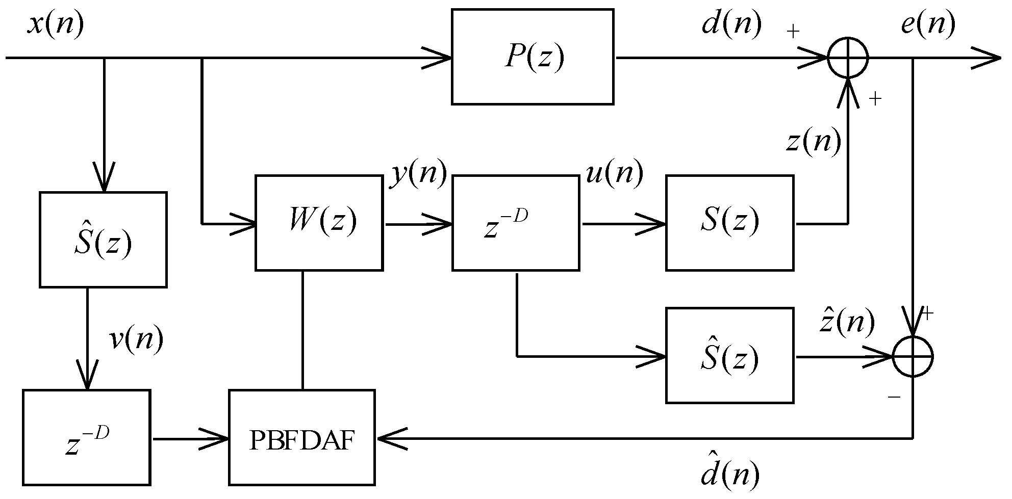
The aforementioned frequency-domain algorithms directly employ the residual error signal $e\left(n\right)$ to update the weight vector, resulting in a delay between the weight adaptation and the observation of the error signal. To reduce this type of delay, the modified filtered-x structure was adopted to update the weight vector in [35], as shown in Figure 3. The basic idea is summarized as follows. The disturbance signal $\widehat{d}\left(n\right)$ at the error microphone is estimated as

$$\widehat{d}\left(n\right)=e\left(n\right)-\widehat{z}\left(n\right)$$

(26)

where

$$\widehat{z}\left(n\right)=u\left(n\right)\ast \widehat{s}$$

(27)

is the estimate of the control signal at the location of the error microphone. To reduce the complexity, the linear convolution in (27) is implemented using FFT. Then, $\widehat{z}\left(n\right),kL-L+1\le n\le kL$ can be computed as

$$\begin{array}{c}\widehat{\mathbf{z}}\left(k\right)={\left[\widehat{z}(kL-L+1),...,\widehat{z}\left(kL\right)\right]}^T\hfill \\ ={\left[u(kL-L+1)\ast \widehat{s},...,u\left(kL\right)\ast \widehat{s}\right]}^T\hfill \\ ={\mathbf{Q}}^{01}{\mathbf{F}}^{-1}\sum _{p=0}^{P_{\mathrm{s}}-1}{\mathbf{U}}_p\left(k\right){\widehat{\mathbf{S}}}_p,\hfill \end{array}$$

(28)

where

$${\mathbf{U}}_p\left(k\right)=diag\left\{\mathbf{F}{\mathbf{u}}_p\left(k\right)\right\}$$

(29)

is the frequency-domain cancelling signal matrix with ${\mathbf{u}}_p\left(k\right)={\{u[(k-p-2)L+1],...,u\left[(k-p)L\right]\}}^T$. The estimated disturbance signal vector is

$$\begin{array}{c}\widehat{\mathbf{d}}\left(k\right)={[\widehat{d}(kL-L+1),...,\widehat{d}\left(kL\right)]}^T\hfill \\ =\mathbf{e}\left(k\right)-\widehat{\mathbf{z}}\left(k\right).\hfill \end{array}$$

(30)

Recall that $\widehat{\mathbf{d}}\left(k\right)$ is generated by ${\mathbf{V}}_p(k-2)$, and the pseudo frequency-domain error vector can be calculated as

$$\widehat{\mathbf{E}}\left(k\right)=\widehat{\mathbf{D}}\left(k\right)+{\mathbf{G}}^{01}\sum _{p=0}^{P_{\mathrm{w}}-1}{\mathbf{V}}_p(k-2){\mathbf{W}}_p\left(k\right),$$

(31)

where

$${\mathbf{G}}^{01}=\mathbf{F}\left[\begin{array}{cc}{\mathbf{0}}_L& {\mathbf{0}}_L\\ {\mathbf{0}}_L& {\mathbf{I}}_L\end{array}\right]{\mathbf{F}}^{-1}$$

(32)

is the overlap-save projection matrix, and

$$\widehat{\mathbf{D}}\left(k\right)=\mathbf{F}{[{\mathbf{0}}_{1\times L},{\widehat{\mathbf{d}}}^T\left(k\right)]}^T$$

(33)

is the reconstructed frequency-domain disturbance signal vector. The pseudo frequency-domain error vector $\widehat{\mathbf{E}}\left(k\right)$ is only used for the weight update. The weight update equation is

$${\mathbf{W}}_p(k+1)={\mathbf{W}}_p\left(k\right)-\mu {\mathbf{G}}^{10}{\mathbf{\Lambda }}^{-1}\left(k\right){\mathbf{V}}_p^H(k-2)\widehat{\mathbf{E}}\left(k\right).$$

(34)

Equations (31) and (34) describe the standard PBFDAF algorithm, which removes the effect of the secondary path. The output of the control filter can be computed using ${\mathbf{W}}_p(k+1)$ according to (25). However, the delay in the signal path still exists. The FPBMFxLMS algorithm is presented in

Table 5. FPBMFxLMS algorithm [35].

Operation	Complexity
(1) Compute the frequency-domain reference matrix ${\mathbf{U}}_0\left(k\right)$ using (29)	One FFT
(2) Estimate the control signal at the error microphone $\widehat{\mathbf{z}}\left(k\right)$ using (28)	One FFT and $4L{P}_{\mathrm{s}}$ multiplications
(3) Estimate the disturbance signal vector $\widehat{\mathbf{d}}\left(k\right)$ using (30)	0
(4) Compute the frequency-domain reference matrix ${\mathbf{X}}_0\left(k\right)$ using (8)	One FFT
(5) Compute the filtered reference signal vector $\mathbf{v}\left(k\right)$ using (11)	One FFT and $4L{P}_{\mathrm{s}}$ multiplications
(6) Compute the FFT of ${\mathbf{v}}_0\left(k\right)$ using (15)	One FFT
(7) Commutate the pseudo frequency-domain error vector $\widehat{\mathbf{E}}\left(k\right)$ using (31)	2 FFT and $4L{P}_{\mathrm{w}}$ multiplications
(8) Update $\mathbf{\Lambda }\left(k\right)$ using (17)	$4L$ multiplications
(9) Update the weight vector using (34)	$2P_{\mathrm{w}}$ FFTs and $6L{P}_{\mathrm{w}}$ multiplications
(10) Compute the control filter out using (25)	One FFT and $4L{P}_{\mathrm{w}}$ multiplications
(11) Compute the cancelling signal using (9) $u\left(n\right)=y(n-2L)$	0

Note: Steps (1)–(10) should be completed between $kL$ and $kL+L$; Average and peak multiplications: $(8+2P_{\mathrm{w}})A/L+14P_{\mathrm{w}}+8P_{\mathrm{s}}$.

.

4. Delayless Frequency-Domain ANC Algorithms

The algorithm in Table 5 removes the delay in the weight update but does not remove the delay in the signal path. It is more essential to remove the delay in the signal path because this delay has a major effect on the performance of broadband ANC systems. Several delayless frequency-domain ANC algorithms have been presented to remove delays in the signal path [44,46,47]. This section first reviews several delayless frequency-domain ANC algorithms, and then, a new delayless algorithm with the modified filtered-x scheme is proposed.

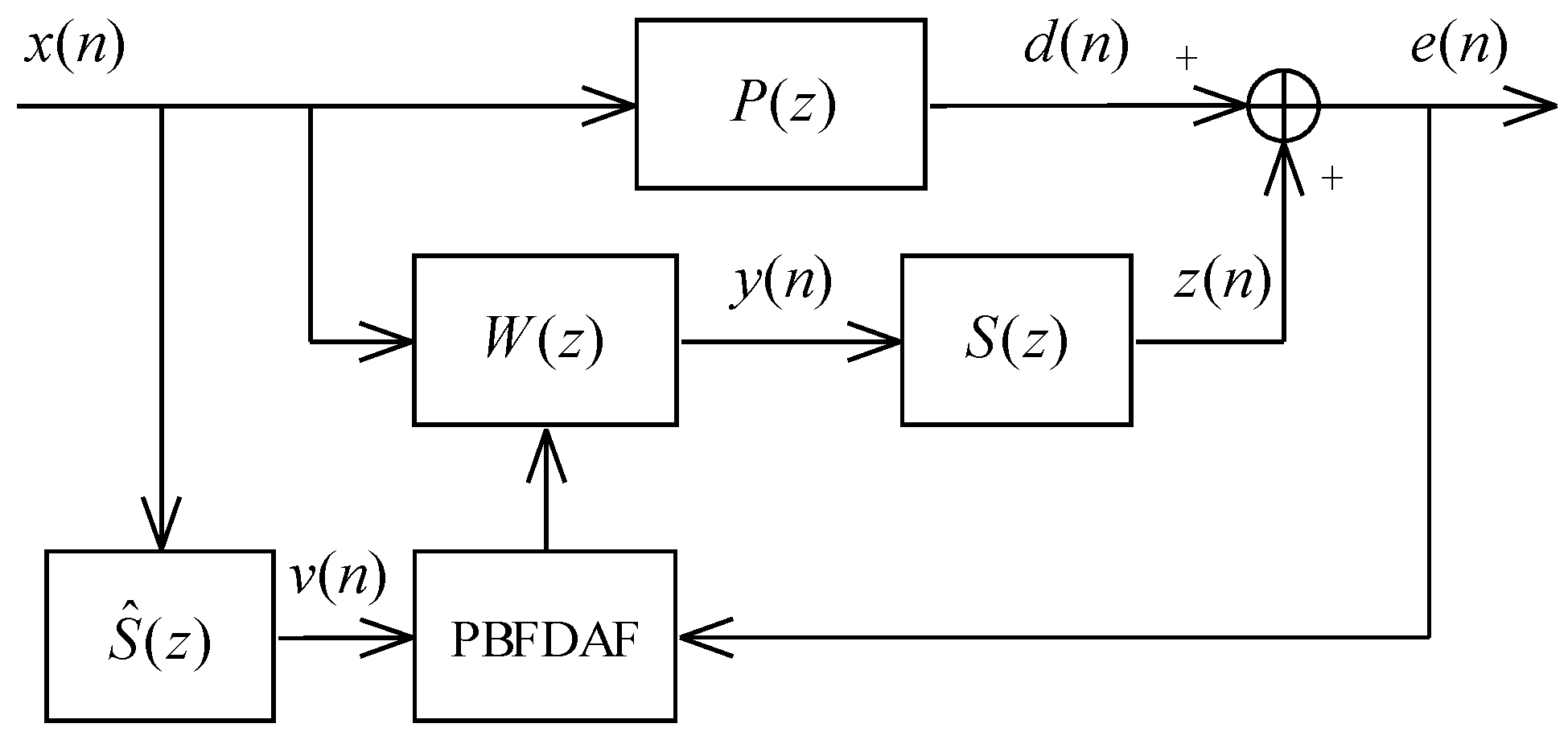
4.1. Qiu’s Delayless Algorithm

The delayless frequency-domain ANC is presented in Figure 4. To avoid the delay in the signal path, the calculation of the adaptive filter output can be directly implemented using the time-domain convolution [40,41,42,43]

$$\mathbf{y}(k+1)=\left[\begin{array}{c}{\mathbf{x}}^T(kL+1)\mathbf{w}(k+1)\\ \cdots \\ {\mathbf{x}}^T(kL+L)\mathbf{w}(k+1)\end{array}\right].$$

(35)

If the filter length $N_{\mathrm{w}}$ is small, the complexity required in (35) may be acceptable. However, when $N_{\mathrm{w}}$ is large, the computational complexity may be too high for a resource-limited system. To resolve this problem, a hybrid fast convolution scheme is adopted to calculate the control filter output [44]

$$\begin{array}{c}\mathbf{y}(k+1)={\left[y(kL+1),...,y(kL+L)\right]}^T\hfill \\ =\left[\begin{array}{c}{\overline{\mathbf{x}}}^T(kL+1){\mathbf{w}}_0(k+1)\\ \cdots \\ {\overline{\mathbf{x}}}^T(kL+L){\mathbf{w}}_0(k+1)\end{array}\right]+\mathrm{\Theta }(k+1),\hfill \end{array}$$

(36)

where $\overline{\mathbf{x}}\left(n\right)={[x\left(n\right),x(n-1),\dots ,x(n-L+1)]}^T$, and

$$\mathrm{\Theta }(k+1)={\mathbf{Q}}^{01}{\mathbf{F}}^{-1}\sum _{p=1}^{P_{\mathrm{w}}-1}{\mathbf{X}}_p(k+1){\mathbf{W}}_p(k+1).$$

(37)

Please note that the calculation of $\mathrm{\Theta }(k+1)$ should be completed between $kL$ and $kL+1$, and the first term of the right-hand side of (36) is calculated in the time domain on a sample-by-sample basis. The update equation is

$${\mathbf{W}}_p(k+1)={\mathbf{W}}_p\left(k\right)-\mu {\mathbf{G}}^{10}{\mathbf{\Lambda }}^{-1}\left(k\right){\mathbf{V}}_p^H\left(k\right)\mathbf{E}\left(k\right).$$

(38)

The calculation of ${\mathbf{w}}_0\left(k\right)$ does not require extra computational cost and is expressed by

$${\mathbf{w}}_0\left(k\right)=\left[{\mathbf{I}}_L\begin{array}{c}\end{array}{\mathbf{0}}_L\right]{\mathbf{F}}^{-1}{\mathbf{W}}_0\left(k\right).$$

(39)

Because the calculation of $\mathrm{\Theta }(k+1)$ uses ${\mathbf{W}}_p(k+1)$, the weight update in (38) should be completed between $kL$ and $kL+1$, which means the update-first approach must be used. By using this approach, the delay in the signal path is removed. However, this algorithm is not practical because (36) and (38) should be completed within one sampling period, which requires $(5+2P_{\mathrm{w}})A+10L{P}_{\mathrm{w}}+4L{P}_{\mathrm{s}}+L$ multiplications per sample. In addition, the algorithm requires L multiplications per sample between $kL+2$ and $kL+L$. Thus, the complexity of the algorithm is not evenly distributed over time, i.e., its peak complexity is rather high. A complexity measurement carried out in [46] indicated that the complexity of this algorithm in the first sample of each block is up to 200 times higher than the mean computational load. Even if a high-performance processor is employed to complete this task, most of this power is wasted. Furthermore, the delay in the weight update still exists, which limits the available step size for adaptation. Qiu’s delayless algorithm is summarized in

Table 6. Qiu’s delayless algorithm [44].

Operation	Complexity
(1) Compute the frequency-domain reference matrix ${\mathbf{X}}_0\left(k\right)$ using (8)	One FFT
(2) Compute the filtered reference signal vector $\mathbf{v}\left(k\right)$ using (11)	One FFT and $4L{P}_{\mathrm{s}}$ multiplications
(3) Compute the FFT of ${\mathbf{v}}_0\left(k\right)$ using (15)	One FFT
(4) Update $\mathbf{\Lambda }\left(k\right)$ using (17)	$4L$ multiplications
(5) Compute the FFT of the error signal using (14)	One FFT
(6) Update the weight vector using (38)	$2P_{\mathrm{w}}$ FFTs and $6L{P}_{\mathrm{w}}$ multiplications
(7) Compute $\mathrm{\Theta }(k+1)$ using (37)	One FFT and $4L(P_{\mathrm{w}}-1)$ multiplications
(8) Compute the cancelling signal $\mathbf{y}(k+1)$ using (36)	$L^2$ multiplications

Note: Steps (1)–(7) should be completed between $kL$ and $kL+1$; Average multiplications: $(5+2P_{\mathrm{w}})A/L+10P_{\mathrm{w}}+4P_{\mathrm{s}}+L$; Peak multiplications: $(5+2P_{\mathrm{w}})A+10L{P}_{\mathrm{w}}+4L{P}_{\mathrm{s}}+L$.

.

4.2. Fink’s Delayless Algorithm

A computationally efficient delayless FDAF algorithm was presented in [46] that uses the fast filtering approach of [48]. The difference between Qiu’s and Fink’s delayless algorithms is twofold. First, the convolutions in the first and second partitions are calculated in the time domain for the Fink’s algorithm. Second, the previous weight vector ${\mathbf{W}}_p\left(k\right)$ instead of ${\mathbf{W}}_p(k+1)$ is used to calculate the control filter output

$$\mathbf{y}(k+1)={\mathbf{y}}_0(k+1)+{\mathbf{y}}_1(k+1)+\mathbf{b}(k+1),$$

(40)

where

$${\mathbf{y}}_p(k+1)={\mathbf{Q}}^{01}{\mathbf{F}}^{-1}{\mathbf{X}}_p(k+1){\mathbf{W}}_p\left(k\right),p=0,1,$$

(41)

$$\begin{array}{c}\mathbf{b}(k+1)={[b(kL+1),...,b(kL+L)]}^T\hfill \\ ={\mathbf{Q}}^{01}{\mathbf{F}}^{-1}{\displaystyle \sum _{p=2}^{P_{\mathrm{w}}-1}}{\mathbf{X}}_p(k+1){\mathbf{W}}_p\left(k\right).\hfill \end{array}$$

(42)

It should be noted that (42) is completed in the k-th frame but not in one sampling period as in Qiu’s algorithm, and hence the high peak complexity is avoided. The elements of ${\mathbf{y}}_0(k+1)$ and ${\mathbf{y}}_1(k+1)$ are computed in the time domain on a sample-by-sample basis

$${\mathbf{y}}_p(k+1)=\left[\begin{array}{c}{\overline{\mathbf{x}}}^T(kL+1-pL){\mathbf{w}}_p\left(k\right)\\ \cdots \\ {\overline{\mathbf{x}}}^T(kL+L-pL){\mathbf{w}}_p\left(k\right)\end{array}\right].$$

(43)

The weight vector is updated using (38), which is completed between $kL+1$ and $kL+L$. Accordingly, the total complexity of the algorithm is distributed evenly in one frame. However, the delay in the weight adaptation is not removed. Fink’s delayless algorithm is presented in

Table 7. Fink’s delayless algorithm [46].

Operation	Complexity
(1) Compute the frequency-domain reference matrix ${\mathbf{X}}_0\left(k\right)$ using (8)	One FFT
(2) Compute the filtered reference signal vector $\mathbf{v}\left(k\right)$ using (11)	One FFT and $4L{P}_{\mathrm{s}}$ multiplications
(3) Compute the FFT of ${\mathbf{v}}_0\left(k\right)$ using (15)	One FFT
(4) Update $\mathbf{\Lambda }\left(k\right)$ using (17)	$4L$ multiplications
(5) Compute the FFT of the error signal using (14)	One FFT
(6) Update the weight vector using (38)	$2P_{\mathrm{w}}$ FFTs and $6L{P}_{\mathrm{w}}$ multiplications
(7) Compute $\mathbf{b}(k+1)$ using (42)	One FFT and $4L(P_{\mathrm{w}}-1)$ multiplications
(8) Compute the cancelling signal $\mathbf{y}(k+1)$ using (40)	$2L^2$ multiplications

Note: Steps (1)–(7) should be completed between $kL$ and $kL+L$; Average and peak multiplications: $(5+2P_{\mathrm{w}})A/L+10P_{\mathrm{w}}+4P_{\mathrm{s}}+2L$.

.

The pipeline of the process should be considered carefully. There are two tasks, the time-domain convolution on a sample-by-sample basis and the frequency-domain procedure on a block-by-block basis. When new block data are collected, the task for the weight update in (38) and the calculation of $\mathbf{b}(k+1)$ are scheduled with low priority and should be completed in one block. When new data are available, the frequency-domain task is interrupted by the time-domain task. Then, the convolution operation is scheduled with high priority and should be completed in one sampling period. After the convolution operation has been executed, the interrupted frequency-domain task is recovered.

4.3. Proposed Delayless Algorithm

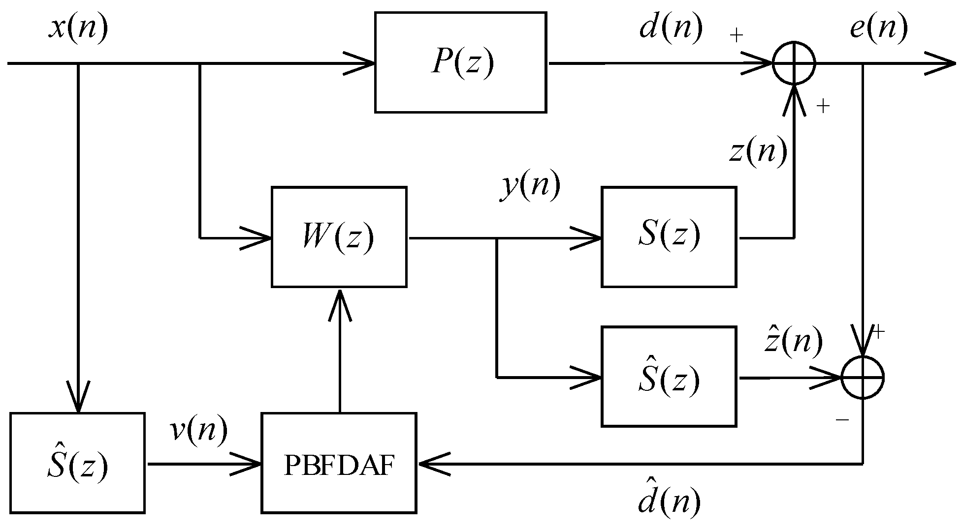
Several approaches have been proposed to remove the delay in the signal path or the weight update delay, but none of these algorithms can remove both kinds of delays. To address this problem, we propose a new delayless frequency-domain FxLMS algorithm as shown in Figure 5. First, we employ the modified filtered-x scheme to the frequency-domain ANC to remove the delay in the weight adaptation. Second, the delayless fast filtering approach in Section 4.2 is used to remove the signal path delay.

The estimate of the control signal at the location of the error microphone is

$$\begin{array}{c}\widehat{\mathbf{z}}\left(k\right)={\left[\widehat{z}(kL-L+1),...,\widehat{z}\left(kL\right)\right]}^T\hfill \\ ={\left[y(kL-L+1)\ast \widehat{s},...,y\left(kL\right)\ast \widehat{s}\right]}^T\hfill \\ ={\mathbf{Q}}^{01}{\mathbf{F}}^{-1}\sum _{p=0}^{P_{\mathrm{s}}-1}{\mathbf{Y}}_p\left(k\right){\widehat{\mathbf{S}}}_p,\hfill \end{array}$$

(44)

where

$${\mathbf{Y}}_p\left(k\right)=diag\left\{\mathbf{F}{\mathbf{y}}_p\left(k\right)\right\}$$

(45)

is the frequency-domain cancelling signal matrix with ${\mathbf{y}}_p\left(k\right)={\{y[(k-p-2)L+1],...,y\left[(k-p)L\right]\}}^T$. Then, we can use (30) to estimate the disturbance signal vector $\widehat{\mathbf{d}}\left(k\right)$. The weight vector is updated as

$$\widehat{\mathbf{E}}\left(k\right)=\widehat{\mathbf{D}}\left(k\right)+{\mathbf{G}}^{01}\sum _{p=0}^{P_{\mathrm{w}}-1}{\mathbf{V}}_p\left(k\right){\mathbf{W}}_p\left(k\right),$$

(46)

$${\mathbf{W}}_p(k+1)={\mathbf{W}}_p\left(k\right)-\mu {\mathbf{G}}^{10}{\mathbf{\Lambda }}^{-1}\left(k\right){\mathbf{V}}_p^H\left(k\right)\widehat{\mathbf{E}}\left(k\right).$$

(47)

Once we obtain the new weight vector ${\mathbf{W}}_p(k+1)$, we can use (40) to calculate the control filter output. By doing so, the delay in the signal path is removed by using the hybrid fast filtering approach, and the delay in the weight update is removed by means of the modified filtered-x structure. Furthermore, the total complexity is distributed evenly in one block, which makes the algorithm practical. The proposed delayless algorithm is presented in

Table 8. Proposed delayless algorithm.

Operation	Complexity
(1) Compute the frequency-domain reference matrix ${\mathbf{X}}_0\left(k\right)$ using (8)	One FFT
(2) Compute the filtered reference signal vector $\mathbf{v}\left(k\right)$ using (11)	One FFT and $4L{P}_{\mathrm{s}}$ multiplications
(3) Compute the FFT of ${\mathbf{v}}_0\left(k\right)$ using (15)	One FFT
(4) Compute the frequency-domain cancelling matrix ${\mathbf{Y}}_0\left(k\right)$ using (45)	One FFT
(5) Estimate the control signal at the error microphone $\widehat{\mathbf{z}}\left(k\right)$ using (44)	One FFT and $4L{P}_{\mathrm{s}}$ multiplications
(6) Estimate the disturbance signal vector $\widehat{\mathbf{d}}\left(k\right)$ using (30)	0
(7) Compute the pseudo frequency-domain error vector $\widehat{\mathbf{E}}\left(k\right)$ using (46)	Two FFTs and $4L{P}_{\mathrm{w}}$ multiplications
(8) Update $\mathbf{\Lambda }\left(k\right)$ using (17)	$4L$ multiplications
(9) Update the weight vector using (47)	$2P_{\mathrm{w}}$ FFTs and $6L{P}_{\mathrm{w}}$ multiplications
(10) Compute $\mathbf{b}(k+1)$ using (42)	One FFT and $4L(P_{\mathrm{w}}-1)$ multiplications
(11) Compute the cancelling signal $\mathbf{y}(k+1)$ using (40)	$2L^2$ multiplications

Note: Steps (1)–(10) should be completed between $kL$ and $kL+L$; Average and peak multiplications: $(8+2P_{\mathrm{w}})A/L+14P_{\mathrm{w}}+8P_{\mathrm{s}}+2L$.

.

5. Computational Complexity Analysis

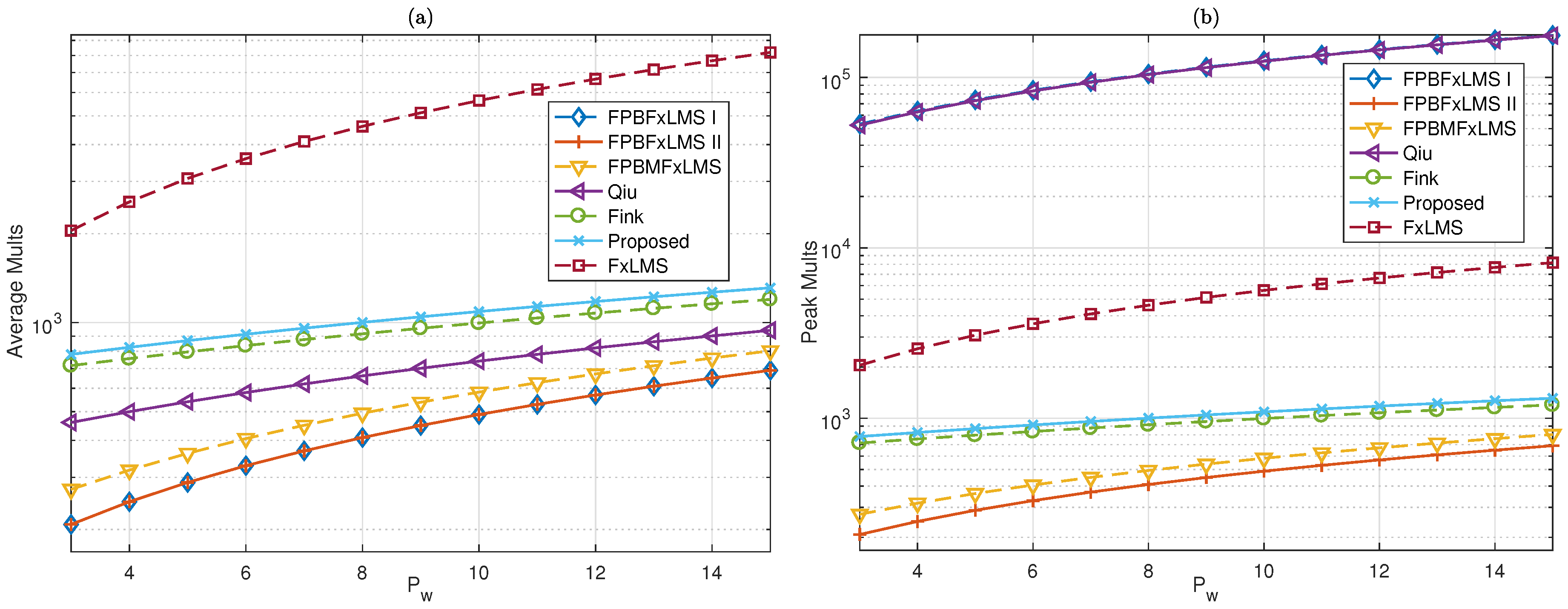
The complexity of the aforementioned frequency-domain FxLMS algorithms is summarized in

Table 9. Complexity of the frequency-domain ANC algorithms.

Algorithm	Average Multiplications per Sample	Peak Multiplications per Sample
FPBFxLMS I [28,37]	$(5+2P_{\mathrm{w}})A/L+10P_{\mathrm{w}}+4P_{\mathrm{s}}$	$(5+2P_{\mathrm{w}})A+10L{P}_{\mathrm{w}}+4L{P}_{\mathrm{s}}+4L$
FPBFxLMS II [39]	$(5+2P_{\mathrm{w}})A/L+10P_{\mathrm{w}}+4P_{\mathrm{s}}$	$(5+2P_{\mathrm{w}})A/L+10P_{\mathrm{w}}+4P_{\mathrm{s}}$
FPBMFxLMS [35]	$(8+2P_{\mathrm{w}})A/L+14P_{\mathrm{w}}+8P_{\mathrm{s}}$	$(8+2P_{\mathrm{w}})A/L+14P_{\mathrm{w}}+8P_{\mathrm{s}}$
Qiu [44]	$(5+2P_{\mathrm{w}})A/L+10P_{\mathrm{w}}+4P_{\mathrm{s}}+L$	$(5+2P_{\mathrm{w}})A+10L{P}_{\mathrm{w}}+4L{P}_{\mathrm{s}}+L$
Fink [46]	$(5+2P_{\mathrm{w}})A/L+10P_{\mathrm{w}}+4P_{\mathrm{s}}+2L$	$(5+2P_{\mathrm{w}})A/L+10P_{\mathrm{w}}+4P_{\mathrm{s}}+2L$
Proposed	$(8+2P_{\mathrm{w}})A/L+14P_{\mathrm{w}}+8P_{\mathrm{s}}+2L$	$(8+2P_{\mathrm{w}})A/L+14P_{\mathrm{w}}+8P_{\mathrm{s}}+2L$

. We assume that one $2L$-point real FFT can be realized using one L-point complex FFT plus additional operations, requiring $2L{log}_2\left(L\right)+4L$ real multiplications [4]. The peak and average multiplications per sample required for the frequency-domain ANC algorithms involved are presented in Figure 6, where we use $L=256$ and $P_{\mathrm{s}}=2$. The average complexity of all the frequency-domain algorithms is lower than that of the FxLMS algorithm, which shows the complexity advantage of the frequency-domain adaptive algorithms. The FPBFxLMS I in [28,37] and Qiu’s delayless algorithm in [44] both have high peak complexity and hence are unrealizable in real-time systems. The proposed delayless method achieves load-balanced implementation and is only slightly more complex than Fink’s delayless algorithm in [46].

6. Evaluations

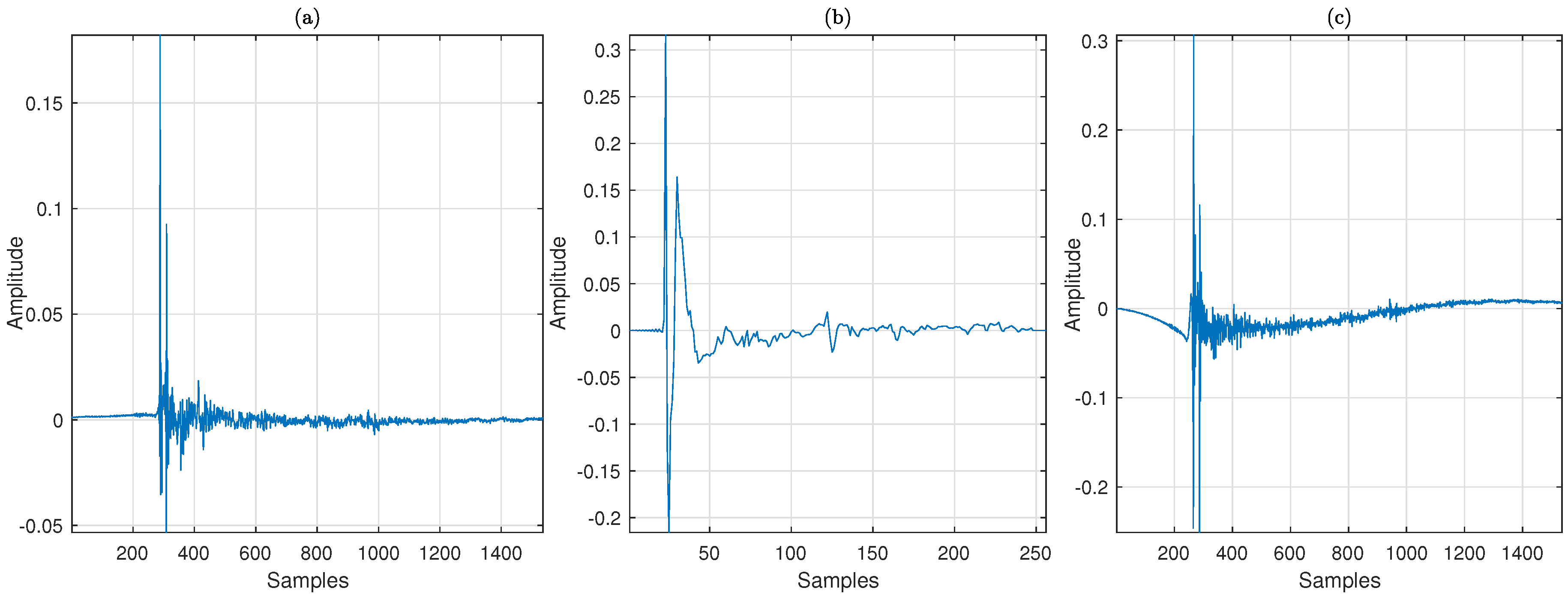
In this section, we carry out computer simulations to evaluate the convergence performance of several frequency-domain algorithms in the context of ANC. The sampling rate is $f_s=32768$ Hz. The length of the primary and secondary path are $N=1536$ and $N_{\mathrm{s}}=256$, respectively. The optimal solution of the control filter is computed using the MINT method [52] and has a length of $N_{\mathrm{w}}=1536$. Their corresponding time-domain impulse responses are plotted in Figure 7. Figure 7c shows that maximum delay allowed in the signal path is $D=256$ to guarantee the causality condition of the system. The signal-to-noise ratio (SNR) measured at the error microphone is 30 dB. Two signals, i.e., the narrow band signal between 100–800 Hz and a multi-tone signal at 40, 340 and 700 Hz, are used as the reference. The convergence performance is evaluated by the learning curve given by

$$A\left(k\right)=10{log}_{10}\left(P_e\left(k\right)/P_d\left(k\right)\right),$$

(48)

where $P_d\left(k\right)$ and $P_e\left(k\right)$ denote the powers of the disturbance signal $d\left(n\right)$ and the error signal $e\left(n\right)$, which are computed recursively as

$$P_d\left(k\right)=\beta P_d(k-1)+(1-\beta )\sum _{n=kL-L+1}^{kL}{d}^2\left(n\right),$$

(49)

$$P_e\left(k\right)=\beta P_e(k-1)+(1-\beta )\sum _{n=kL-L+1}^{kL}{e}^2\left(n\right),$$

(50)

where $\beta$ is the smoothing factor. In the following, we use $\lambda =0.8$ and $\beta =0.8$.

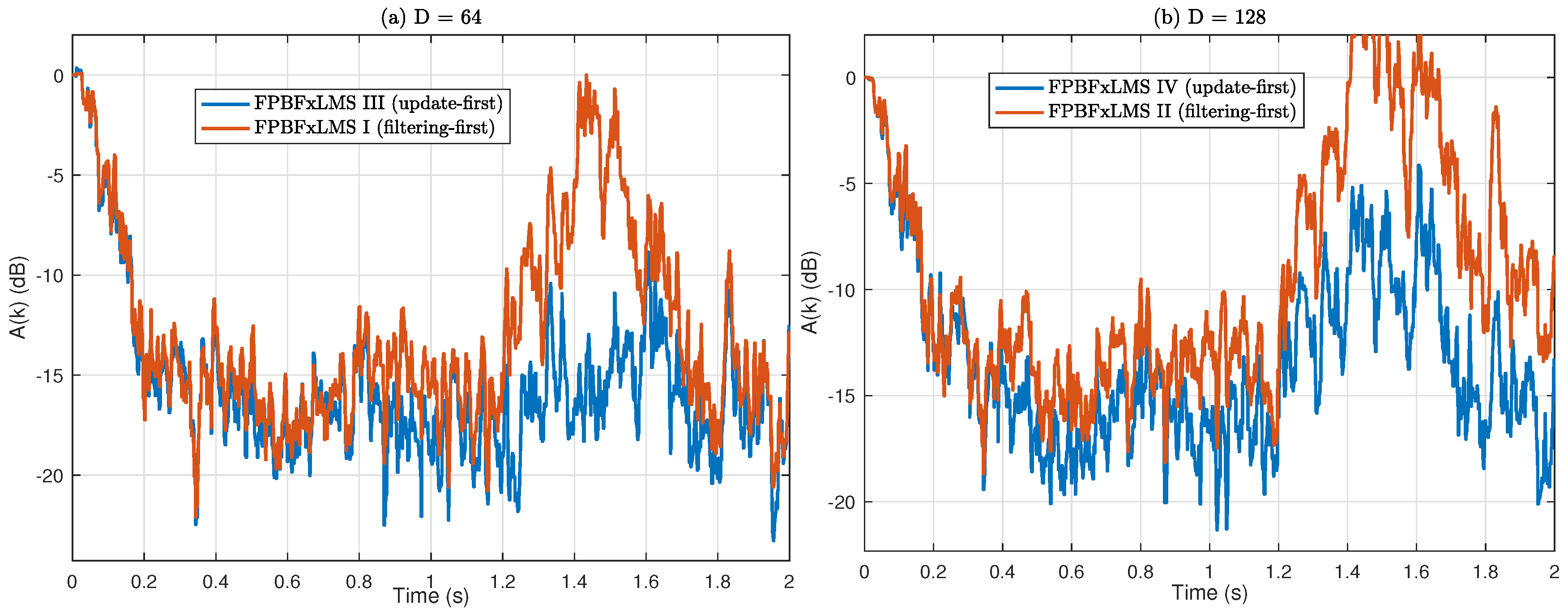
Figure 8 compares the convergence performance of the filtering-first and update-first approaches in Table 1, Table 2, Table 3 and Table 4. The narrow band noise is used as input, and the block length is $L=64$. The update-first approach is more stable than the filtering-first approach given the same step size, which agrees with the above analysis. In addition, the two methods have the same complexity, and hence the update-first approach is recommended for practical implementation.

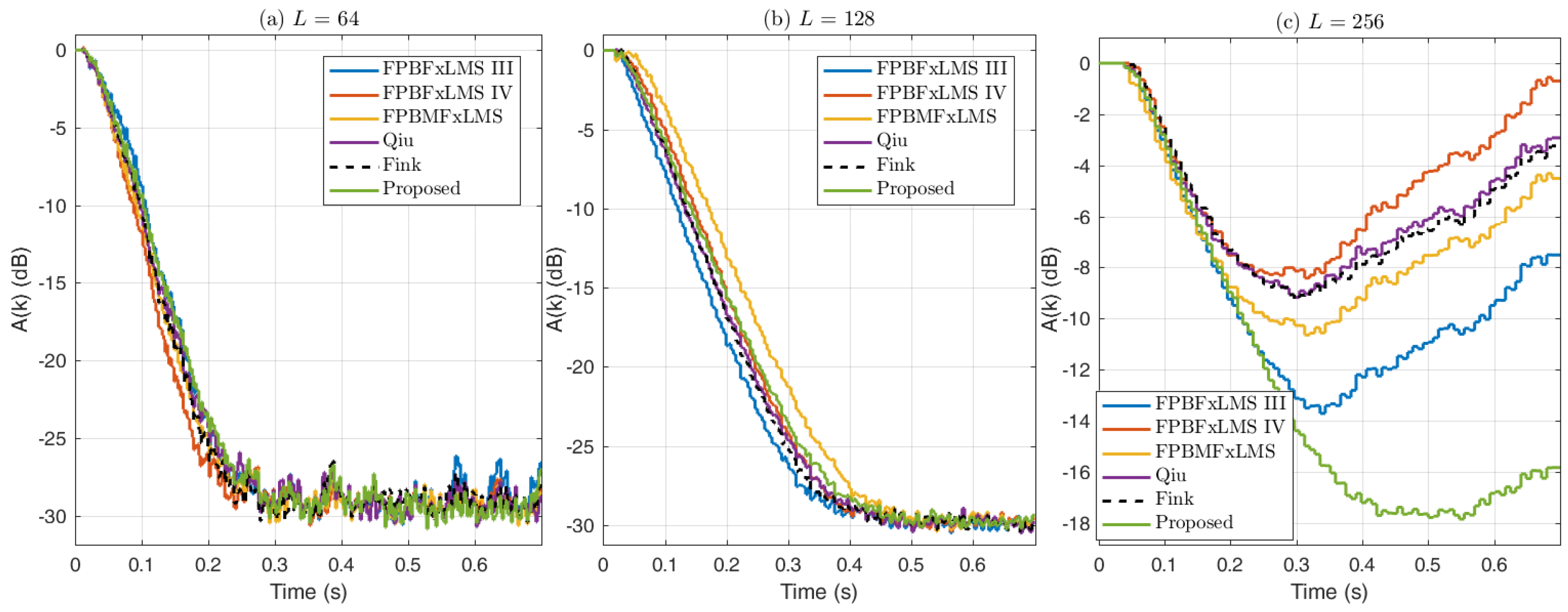
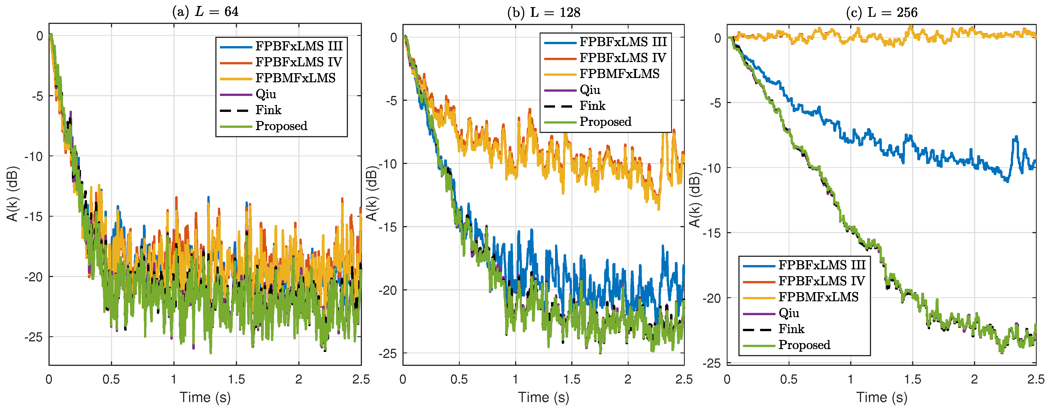
The effect of the block length on the convergence performance of several frequency-domain FxLMS algorithms is investigated in Figure 9 and Figure 10. In Figure 9, we use the multi-tone signal as the reference, and the step size $\mu =0.03$. The block length is set to $L=64,128,256$. All the algorithms are convergent for $L=64,128$, while they diverge for $L=256$. We found that all the algorithms can converge using a smaller step size $\mu =0.001$ for the block length $L=256$. For the multi-tone input, all the frequency-domain algorithms can converge if a sufficiently small step size is employed.

The experiment in Figure 9 is repeated using the narrow band noise as input, and the learning curves are presented in Figure 10. The three delayless frequency-domain algorithms are stable and have a similar convergence for narrow band noise input in all the experiments. However, their convergence rate decreases as the block length. The convergence performance of the traditional frequency-domain FxLMS algorithms is dramatically affected by the block length. For $L=64$, the causality condition is fulfilled for all the algorithm involved, and they exhibit a similar convergence. When the block length is $L=256$, the FPBFxLMS IV and the FPBMFxLMS algorithms with a delay of $D=512$ do not gain any noise reduction, and the FPBFxLMS III algorithm with a delay of $D=256$ only exhibits a 10-dB noise reduction. The experiment demonstrates that the delay in the signal path has a major effect on the broadband noise reduction.

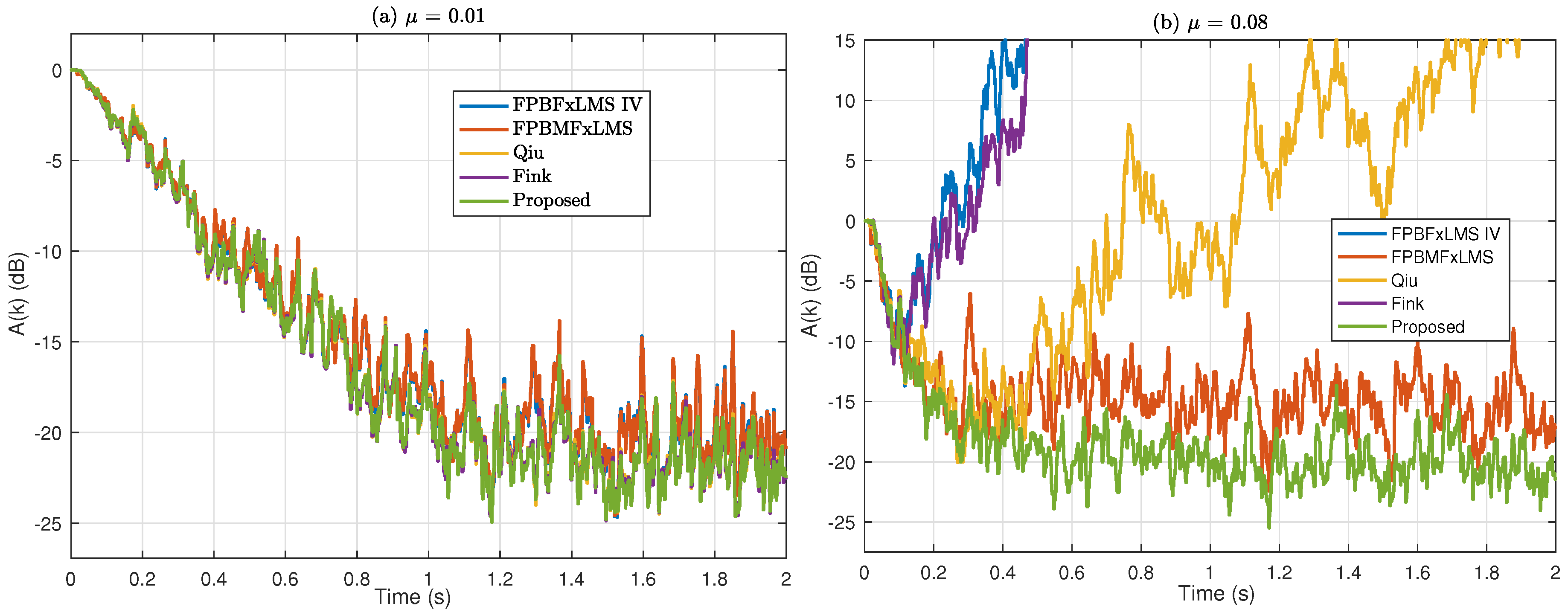
In Figure 11, we investigate the stability of the frequency-domain algorithms with and without the modified filtered-x structure. Specifically, we compare the FPBFxLMS IV, FPBMFxLMS, and three delayless algorithms. The narrow band white noise is used as the reference. We use a small step size $\mu =0.01$ for Figure 11a and a large step size $\mu =0.08$ for Figure 11b. All the algorithms involved exhibit a similar convergence performance when the step size is small. However, when a large step size is adopted, the frequency-domain algorithms without the modified filtered-x structure diverge, but the modified filtered-x algorithms are stable because the available step size of the modified filtered-x algorithm is larger than those of the FxLMS-type algorithms. The proposed delayless algorithm outperforms all the other methods.

7. Conclusions

This paper presented a comprehensive review of the frequency-domain FxLMS algorithms in terms of convergence performance, stability, and computational burden. Practical applications include active noise control of open windows [53], the ventilation system [54], and automotive cabins [55], where several thousands of coefficients are required to model the control filters. The frequency-domain algorithms used in ANC and system identification are quite different. First, broadband ANC is sensitive to algorithm latency, and a large delay may cause the system to fail. Second, direct use of an FDAF for ANC results in a delay in the weight update and the observation of the error signal, which reduces the maximum step size of the algorithm.

This paper reviewed the delayless filtering methods and the modified filtered-x structures to address the two delay problems. Specifically, the update-first approach was proposed to improve the stability of the FPBFxLMS algorithms. Several frequency-domain FxLMS algorithms have a very high peak complexity and thus are not practical for real-time systems, although these algorithms are correct in theory. A computationally efficient delayless frequency-domain algorithm was proposed that combines the hybrid fast filtering approaches and the modified filtered-x structure, which completely removes the aforementioned two types of delays. Extensive simulations were carried out to evaluate the convergence performance of the state-of-the-art frequency-domain FxLMS algorithms.

However, more work needs to be done regarding the frequency-domain FxLMS algorithms. For instance, the step size bound of the traditional frequency-domain FxLMS algorithms in Table 1, Table 2, Table 3 and Table 4 should be determined. Analyzing the statistical convergence behavior of the frequency-domain FxLMS algorithms is an interesting topic [56,57,58,59].

References

- Basner, M.; Babisch, W.; Davis, A.; Brink, M.; Clark, C.; Janssen, S.; Stansfeld, S. Auditory and non-auditory effects of noise on health. Lancet 2014, 383, 1325–1332. [Google Scholar] [CrossRef] [Green Version]
- Minichilli, F.; Gorini, F.; Ascari, E.; Bianchi, F.; Coi, A.; Fredianelli, L.; Licitra, G.; Manzoli, F.; Mezzasalma, L.; Cori, L. Annoyance judgment and measurements of environmental noise: A focus on Italian secondary schools. Int. J. Environ. Res. Public Health 2018, 15, 208–218. [Google Scholar] [CrossRef] [PubMed]
- Nelson, P.; Elliott, S. Active Control of Sound; Academic Press: San Diego, CA, USA, 1992. [Google Scholar]
- Kuo, S.; Morgan, D. Active Noise Control Systems–Algorithms and DSP Implementations; Springer: New York, NY, USA, 1996. [Google Scholar]
- Lee, K.A.; Gan, W.S.; Kuo, S.M. Subband Adaptive Filtering: Theory and Implementation; Wiley: Chichester, UK, 2009. [Google Scholar]
- Kajikawa, Y.; Gan, W.S.; Kuo, S.M. Recent advances on active noise control: Open issues and innovative applications. APSIPA Trans. Signal Inf. Process. 2012, 1, 1–21. [Google Scholar] [CrossRef]
- Ferrer, M.; Gonzalez, A.; de Diego, M.; Piñero, G. Fast affine projection algorithms for filtered-x multichannel active noise control. IEEE Trans. Audio Speech Lang. Process. 2008, 16, 1396–1408. [Google Scholar] [CrossRef]
- Albu, F.; Bouchard, M.; Zakharov, Y. Pseudo-affine projection algorithms for multichannel active noise control. IEEE Trans. Audio Speech Lang. Process. 2007, 15, 1044–1052. [Google Scholar] [CrossRef]
- Yang, F.; Wu, M.; Yang, J.; Kuang, Z. A fast exact filtering approach to a family of affine projection-type algorithms. Signal Process. 2014, 101, 1–10. [Google Scholar] [CrossRef]
- Farhang-Boroujeny, B. Adaptive Filters: Theory and Applications; John Wiley: Hoboken, NJ, USA, 2013. [Google Scholar]
- Clark, G.A.; Mitra, S.K.; Parker, S.R. Block implementation of adaptive digital filters. IEEE Trans. Acoust. Speech. Signal Process. 1981, 28, 584–592. [Google Scholar] [CrossRef]
- Ferrara, E.R. Fast implementation of LMS adaptive filters. IEEE Trans. Acoust. Speech Signal Process. 1980, 28, 474–475. [Google Scholar] [CrossRef]
- Mansour, D.; Gray, A. Unconstrained frequency-domain adaptive filter. IEEE Trans. Acoust. Speech Signal Process. 1982, 30, 726–734. [Google Scholar] [CrossRef]
- Shynk, J.J. Frequency-domain and multirate adaptive filtering. IEEE Signal Process. Mag. 1992, 9, 14–37. [Google Scholar] [CrossRef]
- Sommen, P. Partitioned frequency domain adaptive filters. In Proceedings of the 23rd Asilomar Conference on Signals, Systems and Computers, Pacific Grove, CA, USA, 30 October–1 November 1989; Volume 2, pp. 677–681. [Google Scholar]
- Soo, J.S.; Pang, K.K. Multidelay block frequency-domain adaptive filter. IEEE Trans. Acoust. Speech Signal Process. 1990, 38, 373–376. [Google Scholar] [CrossRef]
- Merched, R.; Sayed, A.H. An embedding approach to frequency domain and subband adaptive filtering. IEEE Trans. Signal Process. 2000, 48, 2607–2619. [Google Scholar] [CrossRef]
- Enzner, G.; Vary, P. Frequency-domain adaptive Kalman filter for acoustic echo control in hands-free telephones. Signal Process. 2006, 86, 1140–1156. [Google Scholar] [CrossRef]
- Yang, F.; Enzner, G.; Yang, J. Statistical convergence analysis for optimal control of DFT-domain adaptive echo canceler. IEEE/ACM Trans. Audio Speech Lang. Process. 2017, 25, 1095–1106. [Google Scholar] [CrossRef]
- Yang, F.; Enzner, G.; Yang, J. Frequency-domain adaptive Kalman filter with fast recovery of abrupt echo-path changes. IEEE Signal Process. Lett. 2017, 24, 1778–1782. [Google Scholar] [CrossRef]
- Yang, F.; Yang, J. Optimal step-size control of the partitioned block frequency-domain adaptive filter. IEEE Trans. Circuits Syst. II 2018, 65, 814–818. [Google Scholar] [CrossRef]
- Lu, C.; Yang, F.; Yang, J. A Frequency-domain Adaptive feedback cancellation algorithm based on convex combination. In Proceedings of the Asia-Pacific Signal and Information Processing Association, Annual Summit and Conference (APSIPA ASC), Kuala Lumpur, Malaysia, 12–15 December 2017; pp. 474–477. [Google Scholar]
- Herbordt, W.; Kellermann, W. Computationally efficient frequency-domain robust generalized sidelobe canceller. In Proceedings of the International Workshop on Acoustic Echo and Noise Control (IWAENC), Tel-Aviv, Israel, 30 August–2 September 2010; pp. 51–54. [Google Scholar]
- Shen, Q.; Spanias, A.S. Time and frequency domain X block LMS algorithms for single channel active noise control. In Proceedings of the 2nd Int. Congr. Recent Developments in Air- and Structure-Borne Sound Vibration, Auburn University, AL, USA, 4–6 March 1992; pp. 353–360. [Google Scholar]
- Reichard, R.M.; Swanson, D.C. Frequency-domain implementation of the filtered-x algorithm with on-line system identification. In Proceedings of the Recent Advances in Active Control of Sound Vibration, Blacksburg, VA, USA, 28–30 April 1993; pp. 562–573. [Google Scholar]
- Shen, Q.; Spanias, A.S. Frequency domain adaptive algorithms for multi-channel active sound control. In Proceedings of the Recent Advances in Active Control of Sound Vibration, Blacksburg, VA, USA, 28–30 April 1993; pp. 755–766. [Google Scholar]
- Shen, Q.; Spanias, A. Time- and frequency-domain X-block least-mean-square algorithms for active noise control. Noise Control Eng. 1996, 44, 281–293. [Google Scholar] [CrossRef]
- Das, D.P.; Panda, G.; Kuo, S.M. New block filtered-x LMS algorithms for active noise control systems. IET Signal Process. 2007, 1, 73–81. [Google Scholar] [CrossRef]
- Das, K.K.; Satapathy, J.K. Frequency-domain block filtered-X NLMS algorithm for multichannel ANC. In Proceedings of the First International Conference on Emerging Trends in Engineering and Technology, Nagpur, Maharashtra, India, 16–18 July 2008; pp. 1293–1297. [Google Scholar]
- Burdisso, R.A.; Vipperman, J.S.; Fuller, C.R. Causality analysis of feedforward controlled systems with broadband inputs. J. Acoust. Soc. Am. 1993, 94, 234–242. [Google Scholar] [CrossRef]
- Kong, X.; Kuo, S.M. Study of causality constraint on feedforward active noise control systems. IEEE Trans. Circuits Syst. II 1999, 46, 183–186. [Google Scholar] [CrossRef]
- Ahn, S.; Voltz, P.J. Convergence of the delayed normalized LMS algorithm with decreasing step size. IEEE Trans. Signal Process. 1996, 44, 3008–3016. [Google Scholar]
- Bjarnason, E. Active noise cancellation using a modified form of the filtered-x LMS algorithm. In Proceedings of the 6th European Signal Processing Conference, Brussels, Belgium, 24–27 August 1992; pp. 1053–1056. [Google Scholar]
- Kim, I.; Na, H.; Kim, K.; Park, Y. Constraint filtered-x and filtered-u least-mean-square algorithm for the active control of noise in ducts. J. Acoust. Soc. Am. 1994, 95, 3379–3389. [Google Scholar] [CrossRef]
- Lorente, J.; Ferrer, M.; de Diego, M.; Belloch, J.A.; Gonzalez, A. GPU implementation of a frequency-domain modified filtered-x LMS algorithm for multichannel local active noise control. In Proceedings of the 52nd Audio Engineering Society International Conference, Guildford, UK, 2–4 September 2013. [Google Scholar]
- Das, D.P.; Rout, N.K.; Panda, G. New partitioned block filtered-X LMS algorithm for active noise control. In Proceedings of the 1st International Conference on Emerging Trends in Signal Processing and VLSI Design, Hyderabad, India, 11–13 June 2010; pp. 112–117. [Google Scholar]
- Rout, N.K.; Das, D.P.; Panda, G. Computationally efficient algorithm for high sampling-frequency operation of active noise control. Mech. Syst. Signal Process. 2015, 56-57, 302–319. [Google Scholar] [CrossRef]
- Lorente, J.; Belloch, J.A.; Ferrer, M.; Gonzalez, A.; Belloch, J.A.; de Diego, M.; Piñero, G.; Vidal, A. Multichannel active noise control system using a GPU accelerator. In Proceedings of the Inter-Noise Conference, New York, NY, USA, 19–22 August 2012; pp. 7768–7780. [Google Scholar]
- Lorente, J.; Ferrer, M.; Diego, M.D.; González, A. GPU implementation of multichannel adaptive algorithms for local active noise control. IEEE/ACM Trans. Audio Speech, Lang. Process. 2014, 22, 1624–1635. [Google Scholar] [CrossRef]
- Kuo, S.M.; Yenduri, R.K.; Gupta, A. Frequency-domain delayless active sound quality control algorithm. J. Sound Vib. 2008, 318, 715–724. [Google Scholar] [CrossRef]
- Morgan, D.R.; Thi, J.C. A delayless subband adaptive filter architecture. IEEE Trans. Signal Process. 1995, 43, 1819–1830. [Google Scholar] [CrossRef]
- Park, S.J.; Yun, J.H.; Park, Y.C.; Youn, D.H. A delayless subband active noise control system for wideband noise control. IEEE Trans. Signal Process. 2001, 9, 892–897. [Google Scholar]
- Wu, M.; Qiu, X.; Chen, G. An overlap-save frequency-domain implementation of the delayless subband ANC algorithm. IEEE Trans. Acoust. Speech Signal Process. 2008, 16, 1706–1710. [Google Scholar] [CrossRef]
- Qiu, X.; Hansen, C.H. Multidelay adaptive filters for active noise control. In Proceedings of the 14th International Congress on Sound and Vibration (ICSV), Cairns, Australia, 9–12 July 2007; pp. 724–732. [Google Scholar]
- Bendel, Y.; Burshtein, D.; Shalvi, O.; Weinstein, E. Delayless frequency domain acoustic echo cancellation. IEEE Trans. Acoust. Speech Signal Process. 2001, 9, 589–597. [Google Scholar] [CrossRef]
- Fink, M.; Kraft, S.; Holters, M.; Zölzer, U. Load-balanced implementation of a delayless partitioned block frequency-domain adaptive filter. In Proceedings of the Workshop Audiosignal-und Sprachverarbeitung, Koblenz, Germany, 24–26 September 2013; pp. 2868–2879. [Google Scholar]
- Sachau, D.; Jukkert, S. Real-time implementation of the frequency-domain FxLMS algorithm without block delay for an adaptive noise blocker. In Proceedings of the ISMA, Leuven, Belgium, 15–17 September 2014; pp. 93–105. [Google Scholar]
- Gardner, S. Efficient convolution without input-output delay. J. Audio Eng. Soc. 1995, 43, 127–136. [Google Scholar]
- Yang, F.; Wu, M.; Yang, J. A computationally efficient delayless frequency-domain adaptive filter algorithm. IEEE Trans. Circuits Syst. II 2013, 60, 222–226. [Google Scholar] [CrossRef]
- McLaughlin, H.J. System and Method for an Efficiently Constrained Frequency-Domain Adaptive Filter. US5526426A, 11 June 1996. [Google Scholar]
- Chan, K.S.; Farhang-Boroujeny, B. Analysis of the partitioned frequency-domain block LMS (PFBLMS) algorithm. IEEE Trans. Signal Process. 2001, 49, 1860–1874. [Google Scholar] [CrossRef]
- Miyoshi, M.; Kaneda, Y. Inverse filtering of room acoustics. IEEE Trans. Acoust. Speech Signal Process. 1988, 36, 145–152. [Google Scholar] [CrossRef]
- Lam, B.; Shi, C.; Gan, W.S. Active noise control systems for open windows: Current updates and future perspectives. In Proceedings of the 24th International Congress on Sound and Vibration, London, UK, 23–27 July 2017. [Google Scholar]
- Larsson, M.; Johansson, S.; Claesson, I.; Håkansson, L. A module based active noise control system for ventilation systems, part I: Influence of measurement noise on the performance and convergence of the filtered-x LMS algorithm. Int. J. Acoust. Vib. 2009, 14, 188–195. [Google Scholar] [CrossRef]
- Samarasinghe, P.N.; Zhang, W.; Abhayapala, T.D. Recent advances in active noise control inside automobile cabins: Toward quieter cars. IEEE Signal Process. Mag. 2016, 33, 61–73. [Google Scholar] [CrossRef]
- Tobias, O.; Bermudez, J.; Bershard, N. Mean weight behavior of the filtered-x LMS algorithm. IEEE Trans. Signal Process. 2000, 48, 1061–1075. [Google Scholar] [CrossRef]
- Carini, A.; Sicuranza, G.L. Transient and steady-state analysis of filtered-x affine projection algorithms. IEEE Trans. Signal Process. 2006, 54, 665–678. [Google Scholar] [CrossRef]
- Ferrer, M.; Gonzalez, A.; de Diego, M.; Piñero, G. Transient analysis of the conventional filtered-x affine projection algorithm for active noise control. IEEE Trans. Audio Speech Lang. Process. 2011, 19, 652–657. [Google Scholar] [CrossRef]
- Wang, T.; Gan, W.S. Stochastic analysis of FXLMS-based internal model control feedback active noise control systems. Signal Process. 2014, 101, 121–131. [Google Scholar] [CrossRef]