Target Speaker Localization Based on the Complex Watson Mixture Model and Time-Frequency Selection Neural Network

1
Key Laboratory of Speech Acoustics and Content Understanding, Institute of Acoustics, Chinese Academy of Sciences, Beijing 100190, China
2
University of Chinese Academy of Sciences, Beijing 100190, China
3
Xinjiang Laboratory of Minority Speech and Language Information Processing, Xinjiang Technical Institute of Physics and Chemistry, Chinese Academy of Sciences, Urumchi 830001, China
*
Author to whom correspondence should be addressed.
Appl. Sci. 2018, 8(11), 2326; https://0-doi-org.brum.beds.ac.uk/10.3390/app8112326
Submission received: 25 October 2018
/
Revised: 18 November 2018
/
Accepted: 19 November 2018
/
Published: 21 November 2018
(This article belongs to the Section Acoustics and Vibrations)
Abstract
:Common sound source localization algorithms focus on localizing all the active sources in the environment. While the source identities are generally unknown, retrieving the location of a speaker of interest requires extra effort. This paper addresses the problem of localizing a speaker of interest from a novel perspective by first performing time-frequency selection before localization. The speaker of interest, namely the target speaker, is assumed to be sparsely active in the signal spectra. The target speaker-dominant time-frequency regions are separated by a speaker-aware Long Short-Term Memory (LSTM) neural network, and they are sufficient to determine the Direction of Arrival (DoA) of the target speaker. Speaker-awareness is achieved by utilizing a short target utterance to adapt the hidden layer outputs of the neural network. The instantaneous DoA estimator is based on the probabilistic complex Watson Mixture Model (cWMM), and a weighted maximum likelihood estimation of the model parameters is accordingly derived. Simulative experiments show that the proposed algorithm works well in various noisy conditions and remains robust when the signal-to-noise ratio is low and when a competing speaker exists.
1. Introduction
Sound Source Localization (SSL) plays an important role in many signal processing applications, including robot audition [1], camera surveillance [2], and source separation [3]. Conventionally, SSL algorithms focus on the task of localizing all active sources in the environment and cannot distinguish a target speaker from competing speakers or directional noises. Nevertheless, there is one speaker of interest in particular that we want to pay attention to in some scenarios, such as when attending to a host speaker or in voice control systems tailored to a master speaker. Retrieving the location of this target speaker, which is defined as Target Speaker Localization (TSL), usually could not succeed without the help of speaker identification [4] or visual information [5].
Popular SSL algorithms are the Generalized Cross-Correlation with Phase Transform (GCC-PHAT) algorithm [6], the Steered Response Power (SRP)-PHAT algorithm [7], which is a generalization of GCC-PHAT for more than two microphones, and the Multiple Signal Classification (MUSIC) algorithm [8]. These algorithms estimate the Direction of Arrival (DoA) by detecting peaks in a so-called angular spectrum. To facilitate localization of speech sources in noisy and reverberant conditions, time-frequency bin weighting methods have been proposed to emphasize the speech components, especially the direct sound components, in the observed signals [9]. These techniques include those based on the signal power [10], the coherent-to-diffuse ratio [11], and the speech presence probability [12].
The motivation behind time-frequency weighting is the sparsity assumption of the signal spectra, or in other words, the assumption that only one source is active in each time frequency bin [13,14]. As suggested in [15], even if the signal is severely corrupted by noises or interferences, there exist target-dominant time-frequency regions that are sufficient enough for localization. It is also found that the human auditory system may perform source separation jointly with source localization [16]. The same motivation lies behind some fairly recent studies that perform robust source localization based on time-frequency masking [17,18,19], in which the authors propose the usage of Deep Neural Networks (DNNs) to perform mask estimation first. The masks are used to weight the narrowband estimates, and the combined algorithms achieve superior performance in adverse environments. Given that mask estimation is a well-defined task in monaural speech separation and large progress has been made with DNN [20], the combination of mask and the SRP-PHAT (or the MUSIC) algorithm is natural and straightforward. Using neural networks, there are also other practices to localize speech sources directly through spatial classification [21,22].
The methods discussed above are directly applicable to TSL if the target speaker is the only speech source in the environment. When a competing speaker exits, multiple source localization techniques [23] could be applied; however, the localization results remain non-discriminative, and further post-processing for speaker identification is needed. TSL in a multi-speaker environment surely requires prior information of the target, such as a keyword uttered by the speaker [24]. Nevertheless, the point is that TSL could be addressed from a different perspective by first performing target speaker separation before localization. The challenge hence is to separate the target speaker from noises and competing interferences. The previous time-frequency masking-based localization algorithms focus on separating speech sources from noise, while not all the speech-dominant bins would be representative of the target speaker. Specifically, in this paper, a speaker-aware DNN is designed to extract the target speaker-dominant time-frequency regions. We also introduce a statistical model, the complex Watson Mixture Model (cWMM), to describe the observations and formulate the localization task as weighted Maximum Likelihood (ML) estimation, rather than investigating the classical SRP-PHAT or MUSIC algorithms.
The cWMM was recently proposed as an alternative to the complex Gaussian Mixture Model (cGMM) for beamforming and blind source separation [25,26]. It is a mixture of Watson distributions. It has also been applied for general source localization [27] and source counting [28] with different spatial directions as states of the distribution. In this paper, we follow the cWMM-based localization technique and apply it to TSL in combination with our time-frequency selection scheme. To extract the target speaker, a Bidirectional Long Short-Term Memory (BLSTM) neural network is leveraged to estimate binary target masks. A short speech segment containing only the target speaker is additionally used as input to an auxiliary network for tuning the hidden layer parameters of the mask selection neural network. In this way, the network obtains speaker-awareness, but remains speaker independent. The output masks indicate the target time-frequency regions that are later integrated with the weight parameter estimation of the cWMM. Simulative experiments are conducted using real recorded Room Impulse Responses (RIRs), and the performance of the proposed method in various environments, especially when a competing speaker exists, is reported.
This paper is organized as follows. Section 2 introduces the signal model and the cWMM employed to describe the directional statistics. Section 3 details the proposed method including the time-frequency bin selection neural network and the weighting parameter estimation of the cWMM. Section 4 presents the experimental setup, the localization results with competing speakers and noises, and discussions regarding the results. Section 5 concludes the paper.
2. Statistical Model
In this section, the signal model in a general environment is first defined. To perform source localization, the directional statistics are calculated from the observed signals, and then, the complex Watson distribution is introduced to derive a maximum likelihood solution.
2.1. Directional Statistics
Let us consider a general reverberant enclosure. The target speaker signal S is captured by an array of M microphones and possibly contaminated by competing interference I and background noise N. In the Short-Time Fourier Transform (STFT) domain, the observed signal is written as:
where t is the time index, f is the frequency index, and , are respectively the multiplicative transfer functions from the target signal and the interference to the m-th microphone. We rewrite (1) in the vector form:
where is the observation vector, is the target transfer function vector, is the interference transfer function vector, and is the noise vector with denoting transpose.
To infer the location of the target speaker from the observations, we rely on the directional statistics, which is defined as:
where denotes the norm. is the normalized observation vector of size that lies on the complex unit hypersphere. It is assumed that signals coming from different spatial directions would naturally form different clusters [26]. Note that the normalizing operation keeps the level and phase differences unchanged between microphones, which are widely-used features for localization. The vector length is discarded because it is mainly caused by the source power.
2.2. Complex Watson Distribution
Divide the acoustic space into K spatial regions and assume that the source, either the target speaker or the interference, is coming from one potential spatial region, TSL is then to infer the region that has the highest target presence probability. To describe the unit-length directional statistics, the complex Watson distribution is introduced. The probability density function is:
where is the confluent hypergeometric function of the first kind, is a spatial centroid satisfying , and is a real-valued concentration parameter that governs the smoothness of the distribution [29]. Higher concentration values result in a peaky kernel, meaning that more weight is put on observations that are close to the centroid, while lower values of lead to smoother score functions, however sacrificing resolution. This distribution features some good properties. Its value is properly normalized, and it naturally accounts for spatial aliasing, because the distance score , which is equivalent to the normalized response of a beamformer, does not change if individual components of are multiplied with . The observation vector is then modeled by a mixture of Watson distributions as:
where the mixture weight is the spatial presence probability in the k-th region at time t and satisfies . Note that we additionally use to model the background noise, which has an even probability of coming from all directions.
For each candidate region, and can be determined through Maximum Likelihood (ML) estimation given training data collected in advance [30]. They are stored as spatial dictionaries for the training environment and applied in further localization tests. In the localization phase, the mixture weights are estimated by the maximization of , and the maximum peak in the weights would coincide with the target source.
3. Proposed Method
In scenarios where competing speakers coexist with the target speaker, false detection would arise when the target is not active or when the interference is too strong, because the probability of the observation vector would show a high value in the direction of the competing speaker, and the maximum of the mixture weights would not always correspond to the target speaker. The proposed solution to this problem is to perform time-frequency selection first. Accordingly, the likelihood function is modified to be:
where is an indicator of the target speaker activity at the bin. The indicator can take the form of a binary mask [20]:
where X denotes the desired target component, which can be the direct sound or the reverberant image of the target speaker, and V denotes all the other undesired components in the observed signal. Here, a decision threshold of 0 dB is used.
3.1. Time-Frequency Selection
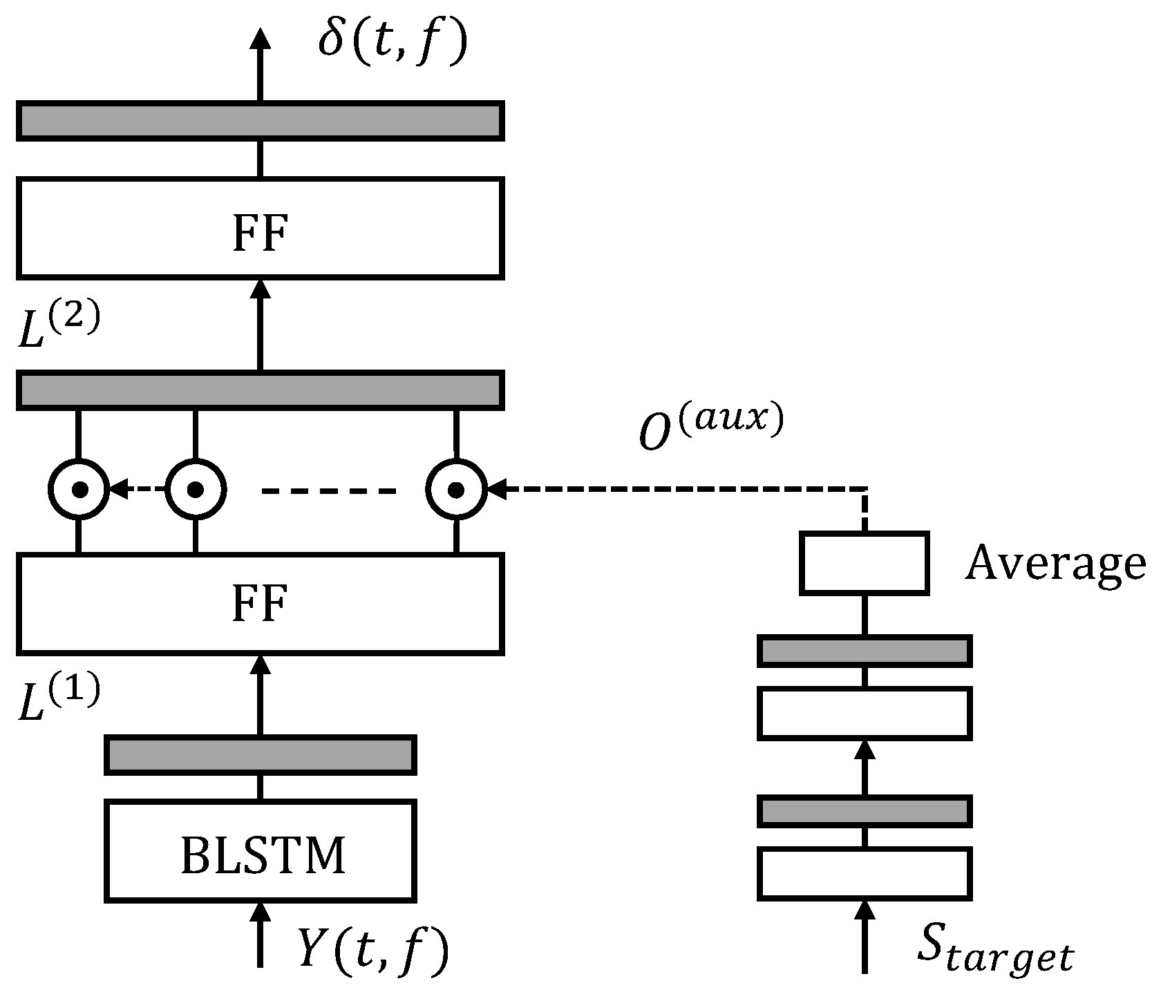
To obtain the target time-frequency masks defined as in Equation (7), we propose a target speaker extractor BLSTM network, which is illustrated in Figure 1. The network consists of one BLSTM layer with 512 nodes followed by two fully-connected Feed-Forward (FF) layers, each with 1024 nodes. This part takes the magnitude spectrum of the observed signal as input and is supposed to output the masks of the target speaker. In our experiments, the Short-Time Fourier Transform (STFT) is performed in 512 points, so the input and output dimensions of the network are both 257. For the last layer, a sigmoid activation function is applied, which ensures that the outputs are in the range of [0,1].
Besides this main network, there is an auxiliary network designed to provide information of the target speaker. The auxiliary network has two fully-connected layers each with 50 nodes and takes a speaker-dependent utterance as input. The frame-level activations of the auxiliary network are averaged over time and serve as utterance-level weights to adapt the second hidden layer outputs of the main network. Mathematically, the computation is expressed as:
where denotes the activations of the l-th layer, is the non-linear activation function, denotes the utterance-averaged weights provided by the auxiliary network, and ⊙ denotes element-wise multiplication. The function of this auxiliary network resembles the Learning Hidden Unit Contribution (LHUC) technique for acoustic model adaptation [31] and the speaker-adaptive layer technique for speaker extraction [32]. In these studies, it has been found that the hidden parameter weighting is better at preserving the speaker information than that using the adaptation utterance as an extra input to the main network.
Given training speech examples, the whole network is optimized under the cross-entropy criterion. The Adam method is applied to schedule the learning process. Weight decay () and weight norm clipping are used to regularize the network parameters. Note that both in the training phase and in the test phase, the neural network is single-channel based, meaning that the target speaker extraction relies only on the spectral characteristics, because the spatial information is not reliable when the competing interference is also speech. Moreover, this setup is flexible, and it is applicable to arbitrary array geometry. In the test phase, we suggest to apply a median pooling on the masks estimated from different channels.
3.2. Weight Parameter Estimation
Once the time-frequency masks of the target speaker are estimated, they can be integrated in the weight parameter estimation of the cWMM together with dictionaries and . In known environments, the spatial dictionaries can be trained using pre-collected data. Though accurate localization is expected in this case, training data collection would be cumbersome. For a general test environment, we consider the direct sound propagation vector [33] as the spatial centroid instead. This vector depends on the array geometry only and is given by:
where j is the complex unit, is the angular frequency, and is the observed delay of the direct sound in the m-th microphone. with the unit vector in the k-th coming direction, the coordinates of the m-th microphone, and c the sound velocity. The concentration parameter is decided through empirical analysis, and we set here, as suggested in [27], which means equal importance is put on different frequencies. For modeling the background noise, is set to zero, which leads to a uniform distribution.
The weight parameters are estimated by the maximization of the weighted likelihood function (6), and this is achieved by the following gradient ascent-based updates [26]:
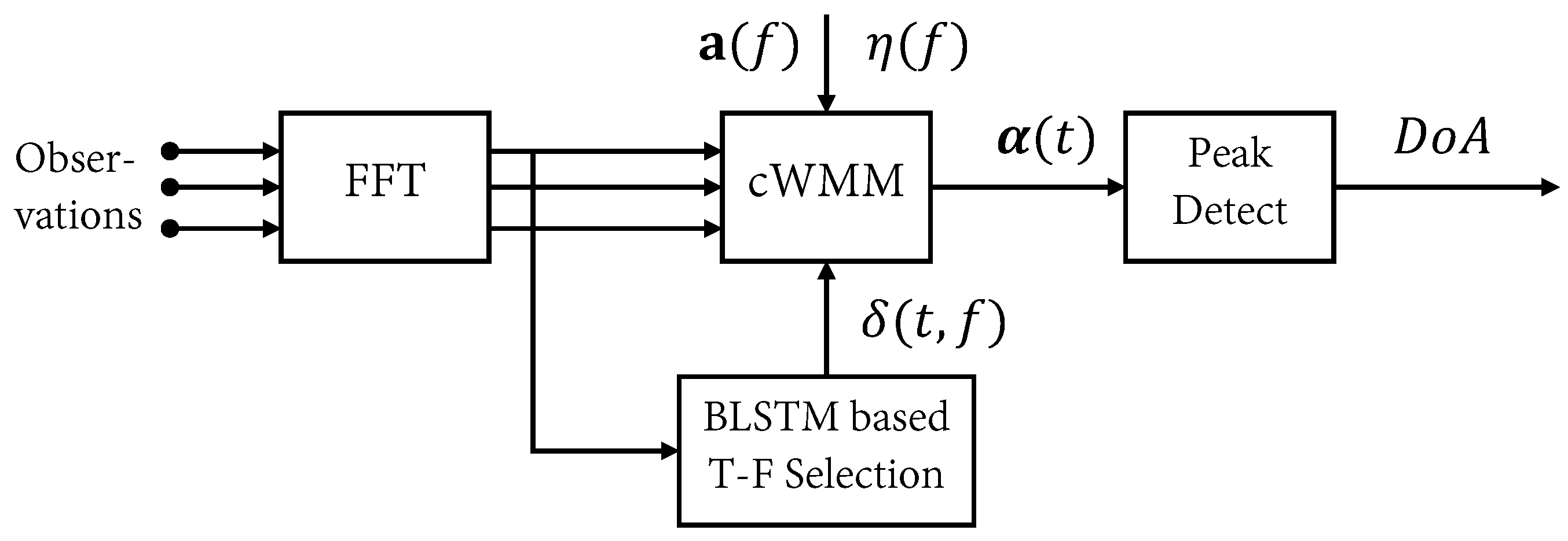
where for initialization, , the learning rate , and the maximum iteration . After the time-frequency selection, the maximum of the mixture weights would correspond only to the target speaker. The processing pipeline of the proposed algorithm is summarized in Figure 2.
4. Experiments
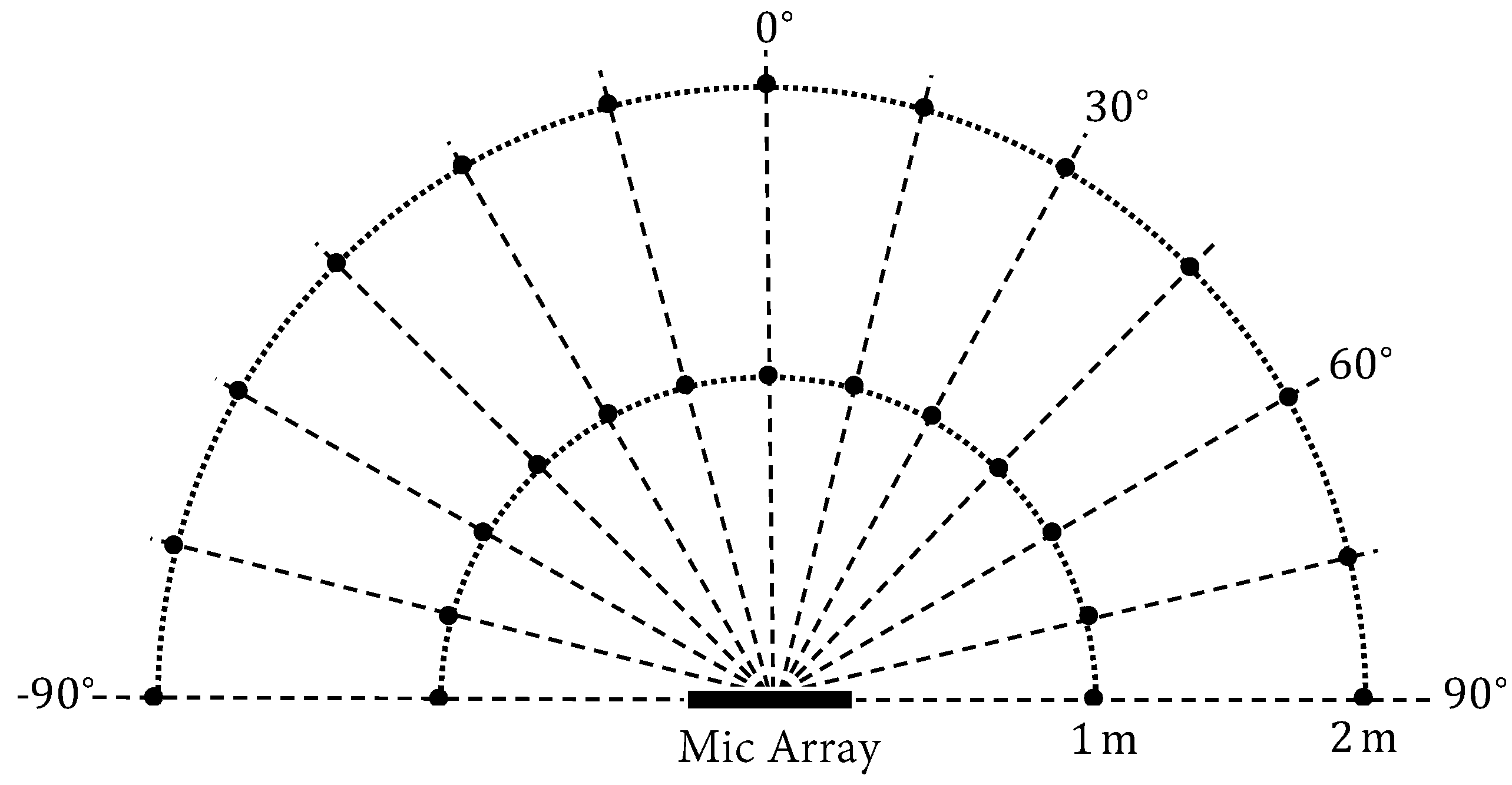
The experiments were conducted in a controlled environment where anechoic speech signals were convolved with real-recorded impulse responses (available at https://www.iks.rwth-aachen.de/en/research/tools-downloads/databases). The speech signals were from the Wall Street Journal (WSJ) corpus [34] and sampled at 16 kHz. The impulse responses were measured in a room with a configurable reverberation level. The reverberation times were set to be 160 ms, 360 ms, and 610 ms. A linear microphone array configuration of eight microphones was used with microphone spacing 3-3-3-8-3-3-3 cm. The source position was set to be 1 m or 2 m away in the azimuth range of in a step. An illustration of the setup is shown in Figure 3.
To generate the test data, speech signals were first randomly drawn from the WSJ development set and the evaluation set. They were truncated to in length for evaluation. The target speaker and one potential interfering speaker were then randomly placed at the black dot positions, as shown in Figure 3, while it was ensured that they were not in the same direction. The microphone observations were a superposition of the reverberant target speaker, reverberant interfering speaker, and background noise. Two types of noise were tested, namely white Gaussian Noise (N0) and spatially-diffuse Noise (N1). The Signal-to-Interference Ratios (SIRs) were set to be −5 dB, 0 dB, and 5 dB. The SIRs were set such that the signal powers of the target speaker were respectively weaker than, equal to, and stronger than that of the competing interference. The Signal-to-Noise Ratios (SNRs) were set to be 20 dB and 30 dB. For each test case, we ran 200 simulations, and we report the results in two different metrics: the Gross Error Rate (GER, in %) and the Mean Absolute Error (MAE, in ). The GER measures the percentage of DoA estimations whose error is larger than a threshold of , and the MAE measures the average estimation bias [24].
For training the target time-frequency selection BLSTM, we used speech signals from the WSJ training set and generated reverberant mixtures with random room and random microphone-to-source distance configurations, following a similar procedure as in [35]. The simulated impulse responses were obtained using a fast implementation of the image source method [36]. In total, there were 20,000 utterances generated for training. The reverberant target speech was used as the reference, and the training target was defined as in Equation (7). The training procedure followed that as described in Section 3.1. For the input to the auxiliary network, a 10-s anechoic utterance containing only the target speaker was applied, which was found to be beneficial for speaker adaptation in the speech recognition task [37]. Note that the clean utterance did not overlap with the test utterances, and it was prepared in advance for each speaker and kept fixed all the time.
4.1. Oracle Investigation
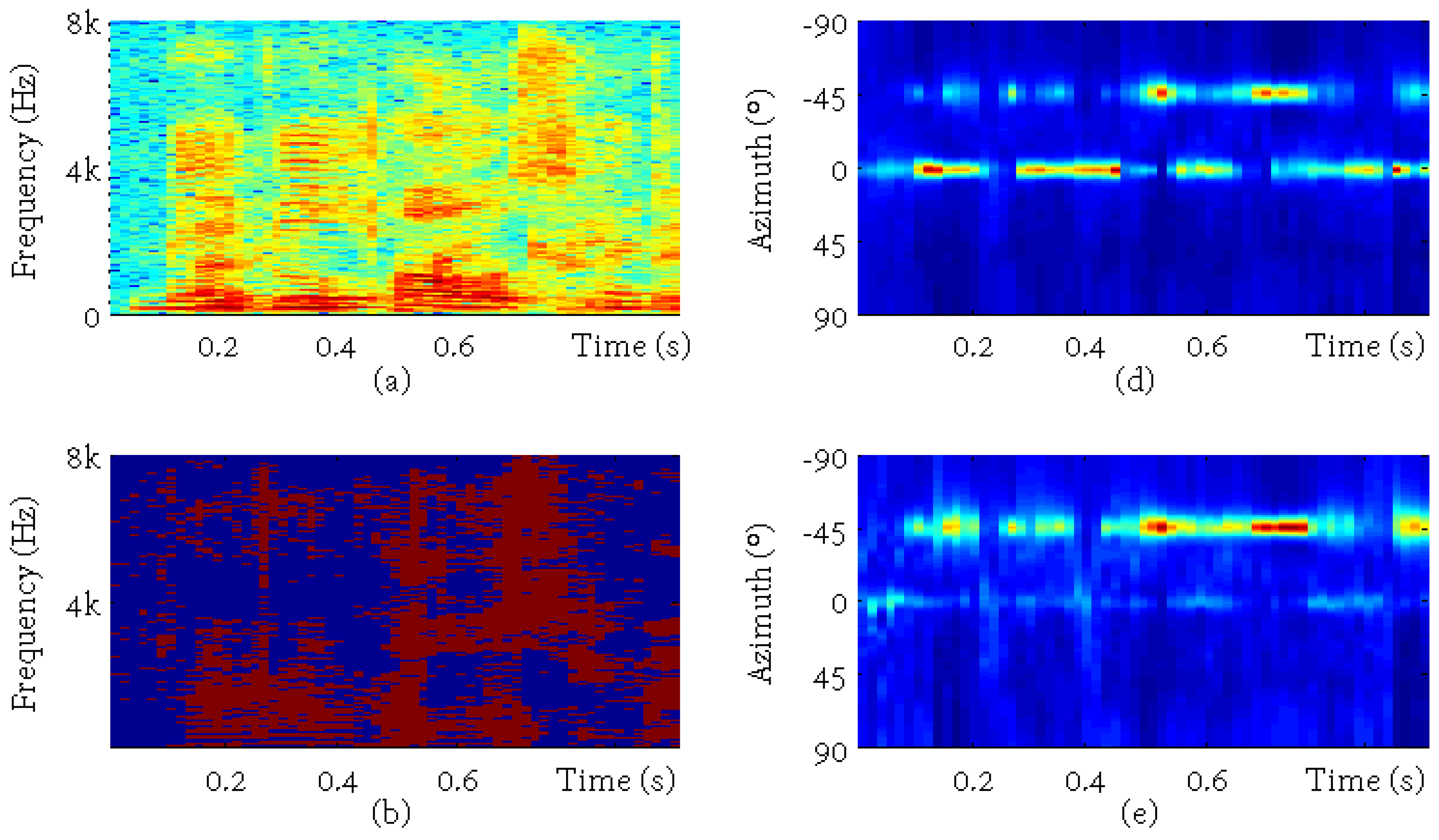
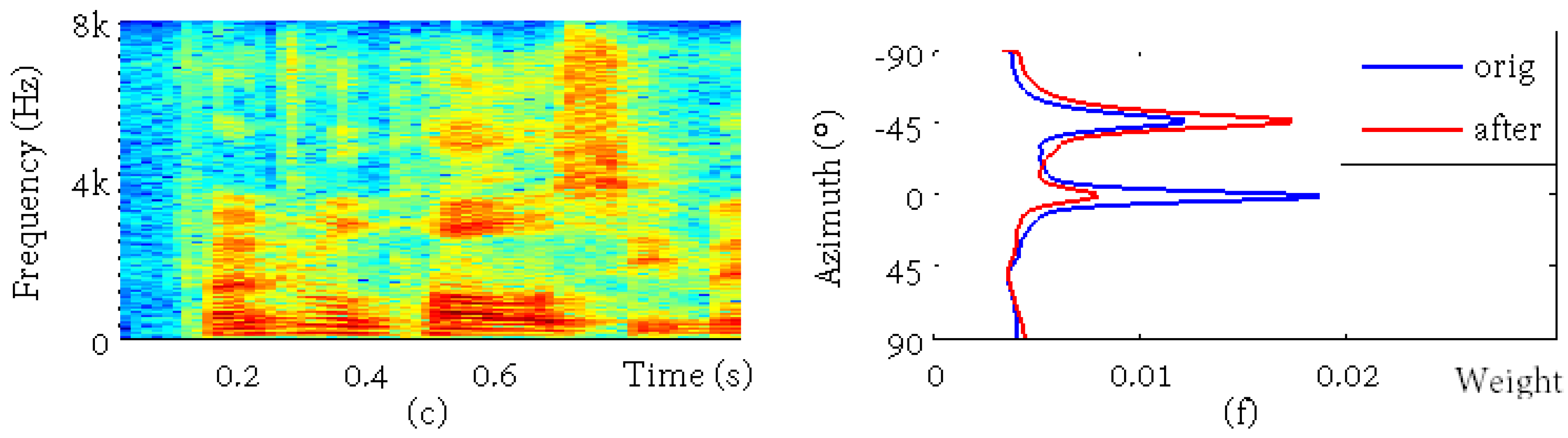
In this part, an example is presented to illustrate the localization results and the effect of time-frequency selection. One test utterance was arbitrarily picked with the target speaker located at −45 and the interference located at 0. The SIR was 0 dB, and the SNR was 30 dB. The sub-figures in Figure 4 are, respectively, (a) the observed mixture spectrum in the first channel, (b) the oracle binary masks for the reverberant target speaker, which were calculated using the reference target and interference signals, (c) the reference reverberant target speech, (d) the cWMM weight parameters for each candidate spatial direction calculated from the multichannel mixture signal, (e) the cWMM weights calculated from the masked mixture signal, and (e) the time-averaged cWMM weights before (the blue curve) and after (the red curve) the binary mask-based time-frequency selection. It is clearly shown that the target masks separated the target speaker from the mixture well and that the maximum of the mixture weights corresponded to the interference before and to the target speaker after the time-frequency selection.
4.2. Performance with Competing Speakers
The experimental results are summarized in terms of GER in Table 1 and in terms of MAE in Table 2. We report the results of the SRP-PHAT algorithm, the original cWMM-based DoA estimation algorithm (cWMM), the cWMM-based algorithm with the target Time-frequency Selection BLSTM network (cWMM-TF), and the cWMM based algorithm using the Oracle target binary mask (cWMM-ORC). A threshold of 0.6 was heuristically chosen to convert the network outputs to binary values. was set to evaluate the source azimuth in a 1 step. The results were averaged over different SNRs.
It is shown that the GER and MAE scores followed similar trends. For both SRP-PHAT and cWMM, there was a general performance degradation as the reverberant time increased, while a special case was the −5 dB SIR, where the GER and MAE were highest in the 160-ms case. The reason was possibly that the less reverberant the mixture was, the higher probability that the estimated DoA corresponded to the stronger interference. Clearly, their performance improved rapidly as the SIR increased. In the case of 0 dB SIR, there was around a 50% GER, meaning that the algorithms could not distinguish the target speaker from the interference without any prior information and just made a guess from the two competing directions, which should be at least 15 away because of the experimental setup. As the SIR went up, the algorithms output the DoA of the stronger source in the mixture, but still, the performance was poor. With the oracle target mask, the cWMM-ORC performed quite robustly in all the test cases and achieved a GER of 8% and an MAE of around 2. The cWMM-ORC was somewhat the upper bound of the cWMM-TF algorithm. Using the masks estimated from the BLSTM network, the cWMM-TF achieved on average 26% GER and 14.54 MAE in the 0-dB SIR case, which were, respectively, a 51% and 55% relative reduction of the original scores without time-frequency selection. The time-frequency selection processing suppressed the interference and effectively benefited the localization accuracy.
4.3. Performance with Competing Noises
This subsection considers the localization performance with only competing noises, since this would be the general case in the acoustic environment. The experiment also indicated the generalization ability of the trained time-frequency selection neural network in unseen scenarios. The MAE results are reported in Table 3 with a subset of the tested environments investigated using a typical reverberation time of 360 ms. The SNRs were set to be 0 dB, 5 dB, and 10 dB. A directional Noise (N2) was also included in evaluation. The noise signal was drawn from the Noisex92 database, and it was then convolved with the measured impulse responses. The localization accuracies differed in different noisy conditions, and as expected, the directional noise affected the performance badly for the SRP-PHAT and cWMM algorithms. The time-frequency selection neural network was able to deal with this case since the information of the target speaker was well kept in the adaptation utterance. Overall, the performance of the algorithms was better than that when an interfering speaker existed. The white noise scenario turned out to be the easiest test case, where the MAEs were around 2–4. Again, the time-frequency selection proved its effectiveness.
4.4. Discussion
One finding is that the cWMM-based localization algorithm performs generally better than the SRP-PHAT algorithm. By looking closely, there are the following differences between the two methods. Rewriting the distance function in Equation (4), , we see that the cWMM-based algorithm also utilizes the cross-channel correlation, but with a global normalization term rather than separately normalizing the correlation coefficients as in SRP-PHAT. The global normalization keeps the original cross-channel level difference, while the separate normalization does not. The cWMM-based localization algorithm applies a concentration parameter for weighting different frequency contributions and properly normalizes its value. The SRP-PHAT algorithm generally treats different frequencies equally.
The other finding is that the time-frequency selection plays an essential part in the localization performance. Localizing a target speaker in a multi-speaker environment would not be successful without additional post-processing using methods such as speaker identification [4] or visual information [5]. The proposed method provides a different solution by first performing separation relying on a reference utterance from the speaker and infers the target location using the established non-discriminative localization methods. The idea of time-frequency weighting has proved its effectiveness for general source localization [17], and it is further validated here. The task of target speaker localization could benefit from this thanks to the recent advances made in monaural speech separation with deep learning techniques [20].
5. Conclusions
The task of localizing a target speaker in the presence of competing interference and background noise is investigated in this paper. A method combining a BLSTM-based target time-frequency selection scheme with the cWMM-based localization algorithm is proposed. The time-frequency neural network additionally relies on a reference utterance from the target and achieves speaker-awareness to predict the target-dominant time-frequency regions in the signal spectra. After time-frequency selection, the general cWMM-based localization method could be applied, and the localization results correspond only to the target. Experiments are conducted in adverse conditions, and the performance of the proposed algorithm remains robust in terms of the GER and MAE metrics.
Combing source separation and source localization as in this paper would facilitate speaker tracking over time, which is another challenging task that could be investigated in future work. For providing the prior information of the speaker to be localized, others speaker-dependent representations, such as pitch and voiceprint, could be introduced to the time-frequency selection neural network.
Author Contributions
Methodology, validation and writing, original draft, Z.W. Review and editing and formal analysis, J.L. Supervision and project administration, Y.Y.
Funding
This work is partially supported by the National Natural Science Foundation of China (Nos. 11461141004, 61271426, U1536117, 11504406, 11590770-4, 61601453), the Strategic Priority Research Program of the Chinese Academy of Sciences (Nos. XDA06030100, XDA06030500, XDA06040603), the National 863 Program (No. 2015AA016306), the National 973 Program (No. 2013CB329302), and the Key Science and Technology Project of the Xinjiang Uygur Autonomous Region (No. 201230118-3).
Conflicts of Interest
The authors declare no conflict of interest.
Abbreviations
The following abbreviations are used in this manuscript:
| cWMM | Complex Watson Mixture Model |
| DNN | Deep Neural Network |
| DoA | Direction of Arrival |
| FF | Feed-Forward layer |
| GCC-PHAT | Generalized Cross-Correlation with Phase Transform |
| GER | Gross Error Rate |
| LHUC | Learning Hidden Unit Contribution |
| LSTM | Long Short-Term Memory |
| MAE | Mean Absolute Error |
| ML | Maximum Likelihood |
| MUSIC | Multiple Signal Classification |
| RIR | Room Impulse Response |
| SIR | Signal-to-Interference Ratio |
| SNR | Signal-to-Noise ratio |
| SRP | Steered Response Power |
| SSL | Sound Source Localization |
| STFT | Short Time Fourier Transform |
| TSL | Target Speaker Localization |
References
- Argentieri, S.; Danès, P.; Souères, P. A survey on sound source localization in robotics: From binaural to array processing methods. Comput. Speech Lang. 2015, 34, 87–112. [Google Scholar] [CrossRef]
- Huang, Y.; Benesty, J.; Elko, G.W. Passive acoustic source localization for video camera steering. In Proceedings of the 2000 IEEE International Conference on Acoustics, Speech, and Signal Processing, Istanbul, Turkey, 5–9 June 2000; Volume 2, pp. II909–II912. [Google Scholar]
- Crocco, M.; Trucco, A. Design of robust superdirective arrays with a tunable tradeoff between directivity and frequency-invariance. IEEE Trans. Signal Process. 2011, 59, 2169–2181. [Google Scholar] [CrossRef]
- May, T.; van de Par, S.; Kohlrausch, A. A binaural scene analyzer for joint localization and recognition of speakers in the presence of interfering noise sources and reverberation. IEEE Trans. Audio Speech Lang. Process. 2012, 20, 2016–2030. [Google Scholar] [CrossRef]
- Busso, C.; Hernanz, S.; Chu, C.W.; Kwon, S.i.; Lee, S.; Georgiou, P.G.; Cohen, I.; Narayanan, S. Smart room: Participant and speaker localization and identification. In Proceedings of the IEEE International Conference on Acoustics, Speech, and Signal Processing (ICASSP ’05), Philadelphia, PA, USA, 23 March 2005; Volume 2. [Google Scholar]
- Knapp, C.; Carter, G. The generalized correlation method for estimation of time delay. IEEE Trans. Acoust. Speech Signal Process. 1976, 24, 320–327. [Google Scholar] [CrossRef]
- DiBiase, J.H.; Silverman, H.F.; Brandstein, M.S. Robust localization in reverberant rooms. In Microphone Arrays; Springer: Berlin/Heidelberg, Germany, 2001; pp. 157–180. [Google Scholar]
- Schmidt, R. Multiple emitter location and signal parameter estimation. IEEE Trans. Antennas Propag. 1986, 34, 276–280. [Google Scholar] [CrossRef]
- Brendel, A.; Huang, C.; Kellermann, W. STFT Bin Selection for Localization Algorithms based on the Sparsity of Speech Signal Spectra. ratio 2018, 2, 6. [Google Scholar]
- Araki, S.; Nakatani, T.; Sawada, H.; Makino, S. Blind sparse source separation for unknown number of sources using Gaussian mixture model fitting with Dirichlet prior. In Proceedings of the IEEE International Conference on Acoustics, Speech and Signal Processing, Taipei, Taiwan, 19–24 April 2009; pp. 33–36. [Google Scholar]
- Braun, S.; Zhou, W.; Habets, E.A. Narrowband direction-of-arrival estimation for binaural hearing aids using relative transfer functions. In Proceedings of the IEEE Workshop on Applications of Signal Processing to Audio and Acoustics (WASPAA), New Paltz, NY, USA, 18–21 October 2015; pp. 1–5. [Google Scholar]
- Taseska, M.; Lamani, G.; Habets, E.A. Online clustering of narrowband position estimates with application to multi-speaker detection and tracking. In Advances in Machine Learning and Signal Processing; Springer: Berlin/Heidelberg, Germany, 2016; pp. 59–69. [Google Scholar]
- Yilmaz, O.; Rickard, S. Blind separation of speech mixtures via time-frequency masking. IEEE Trans. Signal Process. 2004, 52, 1830–1847. [Google Scholar] [CrossRef]
- Ying, D.; Zhou, R.; Li, J.; Yan, Y. Window-dominant signal subspace methods for multiple short-term speech source localization. IEEE/ACM Trans. Audio Speech Lang. Process. 2017, 25, 731–744. [Google Scholar] [CrossRef]
- Woodruff, J.; Wang, D. Binaural localization of multiple sources in reverberant and noisy environments. IEEE Trans. Audio Speech Lang. Process. 2012, 20, 1503–1512. [Google Scholar] [CrossRef]
- Wang, D.; Brown, G.J. Computational Auditory Scene Analysis: Principles, Algorithms, and Applications; Wiley-IEEE Press: Hoboken, NJ, USA, 2006. [Google Scholar]
- Pertilä, P.; Cakir, E. Robust direction estimation with convolutional neural networks based steered response power. In Proceedings of the IEEE International Conference on Acoustics, Speech and Signal Processing (ICASSP), New Orleans, LA, USA, 5–9 March 2017; pp. 6125–6129. [Google Scholar]
- Xu, C.; Xiao, X.; Sun, S.; Rao, W.; Chng, E.S.; Li, H. Weighted Spatial Covariance Matrix Estimation for MUSIC based TDOA Estimation of Speech Source. In Proceedings of the Interspeech 2017, Stockholm, Sweden, 20–24 August 2017; pp. 1894–1898. [Google Scholar]
- Wang, Z.Q.; Zhang, X.; Wang, D. Robust TDOA Estimation Based on Time-Frequency Masking and Deep Neural Networks. In Proceedings of the Interspeech 2018, Hyderabad, India, 2–6 September 2018. [Google Scholar]
- Wang, D.; Chen, J. Supervised speech separation based on deep learning: An overview. IEEE/ACM Trans. Audio Speech Lang. Process. 2018, 26, 1702–1726. [Google Scholar] [CrossRef]
- Xiao, X.; Zhao, S.; Zhong, X.; Jones, D.L.; Chng, E.S.; Li, H. A learning-based approach to direction of arrival estimation in noisy and reverberant environments. In Proceedings of the IEEE International Conference on Acoustics, Speech and Signal Processing (ICASSP), Brisbane, Australia, 19–24 April 2015; pp. 2814–2818. [Google Scholar]
- Takeda, R.; Komatani, K. Discriminative multiple sound source localization based on deep neural networks using independent location model. In Proceedings of the IEEE Spoken Language Technology Workshop (SLT), San Diego, CA, USA, 13–16 December 2016; pp. 603–609. [Google Scholar]
- Li, X.; Girin, L.; Horaud, R.; Gannot, S. Multiple-speaker localization based on direct-path features and likelihood maximization with spatial sparsity regularization. IEEE/ACM Trans. Audio Speech Lang. Process. 2017, 25, 1997–2012. [Google Scholar] [CrossRef]
- Sivasankaran, S.; Vincent, E.; Fohr, D. Keyword-based speaker localization: Localizing a target speaker in a multi-speaker environment. In Proceedings of the Interspeech, Hyderabad, India, 2–6 September 2018. [Google Scholar]
- Vu, D.H.T.; Haeb-Umbach, R. Blind speech separation employing directional statistics in an expectation maximization framework. In Proceedings of the IEEE International Conference on Acoustics Speech and Signal Processing (ICASSP), Dallas, TX, USA, 14–19 March 2010; pp. 241–244. [Google Scholar]
- Ito, N.; Araki, S.; Delcroix, M.; Nakatani, T. Probabilistic spatial dictionary based online adaptive beamforming for meeting recognition in noisy and reverberant environments. In Proceedings of the IEEE International Conference on Acoustics, Speech and Signal Processing (ICASSP), New Orleans, LA, USA, 5–9 March 2017; pp. 681–685. [Google Scholar]
- Drude, L.; Jacob, F.; Haeb-Umbach, R. DOA-estimation based on a complex watson kernel method. In Proceedings of the 23rd European Signal Processing Conference (EUSIPCO), Nice, France, 31 August–4 September 2015; pp. 255–259. [Google Scholar]
- Drude, L.; Chinaev, A.; Vu, D.H.T.; Haeb-Umbach, R. Source counting in speech mixtures using a variational EM approach for complex Watson mixture models. In Proceedings of the 2014 IEEE International Conference on Acoustics, Speech and Signal Processing (ICASSP), Florence, Italy, 4–9 May 2014; pp. 6834–6838. [Google Scholar]
- Mardia, K.; Dryden, I. The complex Watson distribution and shape analysis. J. R. Stat. Soc. Ser. B Stat. Methodol. 1999, 61, 913–926. [Google Scholar] [CrossRef]
- Ito, N.; Araki, S.; Nakatani, T. Permutation-free convolutive blind source separation via full-band clustering based on frequency-independent source presence priors. In Proceedings of the IEEE International Conference on Acoustics, Speech and Signal Processing, Vancouver, BC, Canada, 26–31 May 2013; pp. 3238–3242. [Google Scholar]
- Swietojanski, P.; Li, J.; Renals, S. Learning hidden unit contributions for unsupervised acoustic model adaptation. IEEE/ACM Trans. Audio Speech Lang. Process. 2016, 24, 1450–1463. [Google Scholar] [CrossRef]
- Žmolíková, K.; Delcroix, M.; Kinoshita, K.; Higuchi, T.; Ogawa, A.; Nakatani, T. Learning speaker representation for neural network based multichannel speaker extraction. In Proceedings of the IEEE Automatic Speech Recognition and Understanding Workshop (ASRU), Okinawa, Japan, 16–20 December 2017; pp. 8–15. [Google Scholar]
- Ito, N.; Araki, S.; Nakatani, T. Data-driven and physical model-based designs of probabilistic spatial dictionary for online meeting diarization and adaptive beamforming. In Proceedings of the European Signal Processing Conference (EUSIPCO), Kos, Greece, 28 August–2 September 2017; pp. 1165–1169. [Google Scholar]
- Paul, D.B.; Baker, J.M. The design for the Wall Street Journal-based CSR corpus. In Proceedings of the workshop on Speech and Natural Language, Harriman, NY, USA, 23–26 February 1992; pp. 357–362. [Google Scholar]
- Wang, Z.Q.; Le Roux, J.; Hershey, J.R. Multi-Channel Deep Clustering: Discriminative Spectral and Spatial Embeddings for Speaker-Independent Speech Separation. In Proceedings of the IEEE International Conference on Acoustics, Speech and Signal Processing, Calgary, AB, Canada, 15–20 April 2018. [Google Scholar]
- Allen, J.B.; Berkley, D.A. Image method for efficiently simulating small-room acoustics. J. Acoust. Soc. Am. 1979, 65, 943–950. [Google Scholar] [CrossRef]
- Veselỳ, K.; Watanabe, S.; Žmolíková, K.; Karafiát, M.; Burget, L.; Černockỳ, J.H. Sequence summarizing neural network for speaker adaptation. In Proceedings of the IEEE International Conference on Acoustics, Speech and Signal Processing (ICASSP), Shanghai, China, 20–25 March 2016; pp. 5315–5319. [Google Scholar]
Figure 1.
Architecture of the speaker-aware time-frequency selection neural network. The grey components represent non-linear activations, which are ReLU for the feed-forward layers.
Figure 1.
Architecture of the speaker-aware time-frequency selection neural network. The grey components represent non-linear activations, which are ReLU for the feed-forward layers.

Figure 2.
The processing pipeline of the proposed method.

Figure 3.
The evaluation setup. The black dots mark the positions where the impulse responses are measured.
Figure 3.
The evaluation setup. The black dots mark the positions where the impulse responses are measured.

Figure 4.
An example for oracle investigation. The sub-figures are, respectively, (a) the mixture spectrum, (b) the ideal binary mask of the target, (c) the reference spectrum, (d) the original cWMM weights, (e) the cWMM weights after time-frequency selection, and (f) the averaged weights before (orig) and after (after) processing.


Table 1.
The GER (100%) of the algorithms in different test environments with competing speakers. The bold numbers indicate the best results excluding cWMM-ORC for each SIR. TF, Time-Frequency; ORC, Oracle.
Table 1.
The GER (100%) of the algorithms in different test environments with competing speakers. The bold numbers indicate the best results excluding cWMM-ORC for each SIR. TF, Time-Frequency; ORC, Oracle.
| Noise Type | N0 | N1 | |||||
|---|---|---|---|---|---|---|---|
| SIR | −5 | 0 | 5 | −5 | 0 | 5 | |
| 160 ms | SRP-PHAT | 0.90 | 0.56 | 0.30 | 0.82 | 0.64 | 0.28 |
| cWMM | 0.76 | 0.48 | 0.28 | 0.74 | 0.59 | 0.28 | |
| cWMM-TF | 0.43 | 0.24 | 0.15 | 0.48 | 0.25 | 0.14 | |
| cWMM-ORC | 0.09 | 0.08 | 0.07 | 0.07 | 0.10 | 0.05 | |
| 360 ms | SRP-PHAT | 0.83 | 0.47 | 0.34 | 0.82 | 0.51 | 0.34 |
| cWMM | 0.75 | 0.47 | 0.37 | 0.75 | 0.51 | 0.33 | |
| cWMM-TF | 0.42 | 0.34 | 0.18 | 0.42 | 0.28 | 0.16 | |
| cWMM-ORC | 0.08 | 0.06 | 0.09 | 0.06 | 0.07 | 0.10 | |
| 610 ms | SRP-PHAT | 0.78 | 0.56 | 0.29 | 0.82 | 0.62 | 0.25 |
| cWMM | 0.70 | 0.54 | 0.28 | 0.73 | 0.57 | 0.28 | |
| cWMM-TF | 0.48 | 0.22 | 0.15 | 0.52 | 0.23 | 0.13 | |
| cWMM-ORC | 0.11 | 0.08 | 0.07 | 0.08 | 0.10 | 0.08 | |
Table 2.
The MAE () of the algorithms in different test environments with competing speakers. The bold numbers indicate the best results excluding cWMM-ORC for each SIR.
Table 2.
The MAE () of the algorithms in different test environments with competing speakers. The bold numbers indicate the best results excluding cWMM-ORC for each SIR.
| Noise Type | N0 | N1 | |||||
|---|---|---|---|---|---|---|---|
| SIR | −5 | 0 | 5 | −5 | 0 | 5 | |
| 160 ms | SRP-PHAT | 62.49 | 34.38 | 13.14 | 54.82 | 36.32 | 12.86 |
| cWMM | 55.42 | 32.14 | 16.54 | 49.46 | 39.92 | 17.65 | |
| cWMM-TF | 28.26 | 12.62 | 5.71 | 30.23 | 13.16 | 5.17 | |
| cWMM-ORC | 1.82 | 1.69 | 1.71 | 1.55 | 1.92 | 1.55 | |
| 360 ms | SRP-PHAT | 58.43 | 28.98 | 18.26 | 51.80 | 31.41 | 17.53 |
| cWMM | 53.26 | 29.55 | 23.38 | 47.47 | 32.62 | 19.71 | |
| cWMM-TF | 28.99 | 19.71 | 7.40 | 24.67 | 14.56 | 8.70 | |
| cWMM-ORC | 2.54 | 1.53 | 1.59 | 1.70 | 1.75 | 1.85 | |
| 610 ms | SRP-PHAT | 50.92 | 37.30 | 15.28 | 58.21 | 36.51 | 13.65 |
| cWMM | 45.59 | 37.82 | 15.57 | 52.91 | 37.79 | 17.87 | |
| cWMM-TF | 31.73 | 11.97 | 7.85 | 33.56 | 15.71 | 8.19 | |
| cWMM-ORC | 2.97 | 1.87 | 1.61 | 1.87 | 2.06 | 2.07 | |
Table 3.
The MAE () of the algorithms in different test environments with competing noises.
| Noise Type | N0 | N1 | N2 | |||||||
|---|---|---|---|---|---|---|---|---|---|---|
| SNR | 0 | 5 | 10 | 0 | 5 | 10 | 0 | 5 | 10 | |
| 360 ms | SRP-PHAT | 3.94 | 3.92 | 3.22 | 16.01 | 7.65 | 6.28 | 59.53 | 46.04 | 23.22 |
| cWMM | 2.70 | 1.84 | 1.30 | 28.08 | 10.28 | 5.55 | 53.41 | 38.65 | 24.03 | |
| cWMM-TF | 2.18 | 1.97 | 1.52 | 10.22 | 6.01 | 3.95 | 23.81 | 12.97 | 10.12 | |
| cWMM-ORC | 1.94 | 1.92 | 1.50 | 5.32 | 2.83 | 2.51 | 2.09 | 2.02 | 1.66 | |
© 2018 by the authors. Licensee MDPI, Basel, Switzerland. This article is an open access article distributed under the terms and conditions of the Creative Commons Attribution (CC BY) license (http://creativecommons.org/licenses/by/4.0/).
Share and Cite
MDPI and ACS Style
Wang, Z.; Li, J.; Yan, Y. Target Speaker Localization Based on the Complex Watson Mixture Model and Time-Frequency Selection Neural Network. Appl. Sci. 2018, 8, 2326. https://0-doi-org.brum.beds.ac.uk/10.3390/app8112326
AMA Style
Wang Z, Li J, Yan Y. Target Speaker Localization Based on the Complex Watson Mixture Model and Time-Frequency Selection Neural Network. Applied Sciences. 2018; 8(11):2326. https://0-doi-org.brum.beds.ac.uk/10.3390/app8112326
Chicago/Turabian StyleWang, Ziteng, Junfeng Li, and Yonghong Yan. 2018. "Target Speaker Localization Based on the Complex Watson Mixture Model and Time-Frequency Selection Neural Network" Applied Sciences 8, no. 11: 2326. https://0-doi-org.brum.beds.ac.uk/10.3390/app8112326
Note that from the first issue of 2016, this journal uses article numbers instead of page numbers. See further details here.