Combustion State Recognition of Flame Images Using Radial Chebyshev Moment Invariants Coupled with an IFA-WSVM Model

Abstract

Accurate combustion state recognition of flame images not only plays an important role in social security, but also contributes to increasing thermal efficiency and product quality. To improve the accuracy of feature extraction and achieve the combustion state recognition, a novel method based on radial Chebyshev moment invariants (RCMIs) and an improved firefly algorithm-wavelet support vector machine (IFA-WSVM) model is proposed. Firstly, the potential flame pixels and the potential flame contour are obtained in the pre-processing phase. Then, the rotation, translation and scaling (RTS) invariants of radial Chebyshev moments are derived. Combing the region and contour moments, the RCMIs of pre-processed and edge images are calculated to construct multi-feature vectors. To enhance the recognition performance, an IFA-WSVM model is built, where the IFA is applied to search the best parameters of WSVM. Then, the IFA-WSVM model is used to recognize the combustion state. Finally, the result for case studies show that the proposed method is superior to methods based on HMIs and ZMIs, achieving the highest rate of 99.07% in real time. The IFA algorithm also outperforms other benchmark algorithms. Even for the images transformed by RTS and small size of training sets, the proposed method continues to exhibit the best performance.

1. Introduction

Various kinds of natural disasters and man-made disasters pose serious threats to human lives and property, among which fire is one of the most serious hazards. Rapid flame recognition and early warning can greatly reduce the damage to people’s health and property safety, hence they have drawn worldwide attention. On the other hand, fire plays an important role in energy, power, chemical, metallurgical and other basic industries, contributing to developing human’s civilization and improving product quality. Meanwhile, the unsteady combustion state can decrease thermal efficiency, increase emissions, cause flame extinction and even explosion. Consequently, there is no doubt that a reliable and effective method for the combustion state recognition of flame images is needed.

In regards to traditional recognition technologies, the most frequently used methods are smoke sensors, temperature sensors and gas sensors, which recognize the flame through its physical characteristics, such as solid particles, temperature and the release of CO and CO₂ [1,2,3]. However, these methods all require the sensors to keep a certain distance from the flame. Optical sensors, such as photosensitive sensors and infrared sensors, have the advantages of quick response and long recognition distance. However, they are sometimes difficult to deploy such as outdoor locations and large open facilities.

With the continuous development of image processing technology, video-based flame recognition (VFR) has attracted much attention, depending on its obvious advantages. Compared with traditional methods, VFR can recognize the flame itself directly through extracting the features of flame images, such as motion, edge blurring, color and spatial difference. Rosario et al. [4] used YUV color space to select the suspected flame region. Then according to the diffusion characteristics of flame, the effective detection of flame region was achieved based on the displacement vector variation of SIFT feature points. Zhang et al. [5] introduced probability analysis into the flame detection, the flame region was decided by calculating the RGB distribution in the specified grid. The final flame detection was realized by the change of suspicious region in the two continuous images. Duong et al. [6] proposed a method based on the changes of the statistical features in the flame region between different frames. The final result was obtained by Bayes classifier and defined as fire-alarm rate for each frame. Shao et al. [7] developed a method for flame region detection, which was achieved by introducing the Codebook background model into the YUV color space and extracting the dynamic and static multi-features. A method based on the edge information of flame was proposed in Reference [8], indicating whether the potential area was a flame region or not. Wang et al. [9] proposed a fire smoke detection algorithm based on optical flow method and texture feature, which could be used for early fire alarm. Several researchers also have theoretically investigated that the local binary pattern (LBP) [10,11], Wald-Wolfowitz random test algorithm [12], and convolutional neural network [13] were suitable for flame image detection. Unfortunately, just like the above, most of the existing methods only aim to indicate whether a frame contains flame or not, rather than the combustion state of flame. Although the location, size, color, shape and other features of the flame can reflect the combustion state, it is difficult to describe the combustion state with an exact mathematical model. Therefore, these methods of flame recognition may not be directly used for combustion state recognition.

There are also several studies on combustion state recognition. Lin et al. [14] presented a simple on-line method for the flame image-based burning state recognition, through comparing the structural similarity (SSIM) indexes between the measured image and reference images. However, the main drawback of SSIM is that it is highly sensitive to rotation, translation and scaling of images, which are typically brought about by the movement of the video cameras. Cheng et al. [15] put forward a method using complex wavelet structural similarity (CW-SSIM) to recognize the burning state of rotary kiln. Although the CW-SSIM is robust to small rotation, translation and scaling of images, it still cannot solve the practical problem completely.

In terms of combustion state recognition, artificial intelligence (AI) technologies have been widely used for flame image recognition [16,17,18,19]. Owing to the non-parametric characteristic, AI technologies have a major advantage of requiring no priori concept for the relationships between the input variables and output data [20]. Support vector machine (SVM) was first proposed by Vapnik [21], in accordance with the foundation of statistical theory and the principle of structural risk minimization. Among the existing AI technologies, SVM has been proved to have superior performance over previously developed methodologies, such as decision tree, artificial neural network and other conventional statistical models [22,23,24,25].

Although effective in recognition, the SVM model has a weakness that its performance greatly depends on the parameter selection, which is troublesome and time-consuming for manual operation. To improve the performance and work efficiency, various optimizing algorithms have been introduced into the SVM model, such as genetic algorithm (GA) [26,27] and particle swarm optimization (PSO) [28,29]. Recently, another intelligent optimization method, fire algorithm (FA) proposed by Yang [30] has become a promise in optimization problems. To our best knowledge, there are few studies applying FA to obtain the optimal parameters of SVM. However, the traditional FA often suffers from being trapped into local optimum, which causes a premature problem.

This paper aims to realize the combustion state of flame images coupling radial Chebyshev moment invariants (RCMIs) and improved firefly algorithm-wavelet support vector machine (IFA-WSVM) model. Firstly, the potential flame pixels are segmented from candidate images in the YCbCr color space, and the potential flame contour is extracted by the Canny edge detector. Then, the proposed rotation, translation and scaling (RTS) invariants of radial Chebyshev moments are derived. Next, the RCMIs are calculated to extract the local and global multi-features of candidate images, forming feature vectors. In order to enhance the performance of combustion state recognition, the FA is applied to search the best penalty factor and dilation parameter of SVM model with a Morlet wavelet kernel. Due to the defect of the traditional FA, an improved FA algorithm is proposed to increase the convergence rate and adjust the searching step dynamically. Afterwards, the IFA-WSVM model is utilized to recognize the combustion state of the testing set. To illustrate the performance of proposed method, the comparison with the methods based on HMIs and ZMIs is performed. In addition, a comparison of IFA with traditional FA, GA and PSO is also performed, observing its quality of solution. Finally, the results for case studies demonstrate that the proposed method can increase the recognition rate and achieve the highest rate of 99.07%. The methods combining region moment invariants and contour moment invariants outperform those based on region moment invariants, improving the accuracy of feature extraction. They can also recognize the combustion state in real time, consuming less computational resources. Besides this, the developed IFA can enhance potential solution of optimization, which is superior to other benchmark algorithms. For the images transformed by RTS and small training sets, the proposed method maintains the best recognition performance, proving its validity and stability.

2. Feature Selection Using Radial Chebyshev Moment Invariants

2.1. Pre-Processing of Candidate Image

In the pre-processing phase, the potential flame pixels are segmented from candidate images. Most of the approaches on flame pixels detection are based on color information and the relationship between the different components. In general, the colors of a flame region are between red and yellow. As a result, the RGB color space is widely used. However, the methods based on RGB color space are easily affected by flame color-like objects, such as the setting sun, red flags and so on, increasing the false alarm rate.

As is commonly known, the flame region is generally brighter than the neighborhood in the observed scene. This visual property can be used to detect the existence of flame pixels. YCbCr color space has the ability to separate the luminance from the chrominance, which is more effective than other color spaces such as RGB [31,32]. Meanwhile, most of the image acquisition devices provide output in RGB color space. According to the ITU-R BT.601 standards for standard-definition television, YCbCr color space can be derived from RGB color space as follows [33].

As the brightest region in the scene, the luminance of a flame region should be greater than the mean of luminance of all the pixels. On the other hand, the Chrominance Blue should be less than the values of luminance and Chrominance Red. In our case studies, the rules to detect flame pixels are proposed as follows:

$$\begin{array}{c}I\left(x,y\right)=\{\begin{array}{l}1, if\{\begin{array}{l}Y\left(x,y\right)>1.2Y_{mean}\hfill \\ Y\left(x,y\right)>Cb\left(x,y\right)\hfill \\ Cr\left(x,y\right)>Cb\left(x,y\right)\hfill \end{array}\hfill \\ 0, otherwise\hfill \end{array}\\ Y_{mean}=\frac{1}{S}{\displaystyle \sum _{i=1}^{S}Y\left(x_i,y_i\right)}\end{array}$$

(1)

where $I\left(x,y\right)$ is a binary image representing the existence of flame in a pixel location $\left(x,y\right)$ by 1 and non-existence by 0, $Y_{mean}$ is the mean of luminance of all the pixels, $S$ is the total number of all the pixels in a frame image.

Furthermore, it is noted that the shape feature of a flame is composed of external contour and internal region. The former is the local feature, containing finer details of the shape. The latter is the global feature, containing general features of the shape. However, as region-based descriptors, image moments generally just use all the pixels within a shape. In order to take advantage of local features, the Canny edge detector [34] is used to extract the potential flame contour from pre-processed images $I\left(x,y\right)$. Finally, the edge images $I_e\left(x,y\right)$ are also generated, which contribute to obtaining the boundary-based descriptors.

2.2. Radial Chebyshev Moments

Radial moments are generally expressed in polar coordinates $\left(r,\theta \right)$, and combine a one-dimensional polynomial basis with a circular-harmonic function to construct moments of an image $f\left(r,\theta \right)$. From the mathematical point of view, moments are “projections” of a function onto a polynomial basis [35]. However, in digital image processing, the radial moment has to be converted from the continuous to the discrete domain. For an image of size $N\times N$ pixels, the parameter $r$ is allowed to vary from 0 to $N/2$, and the angle $\theta$ is allowed to vary from 0 to $2\pi$. Consequently, the radial moment of an image of order $p$ and repetition $q$ is generally constructed in the following expression:

$$R_{pq}=n_{pq}{\displaystyle \sum _{r=0}^{m-1}{\displaystyle \sum _{l=0}^{n-1}{\phi }_{pq}\left(r,\theta \right)f\left(r,\theta \right)}}$$

(2)

where $n_{pq}$ is the normalizing factor; $p, q$ are non-negative integers, $0\le p,q\le N-1$; $m=N/2$; $\theta =2\pi l/n$ with $0\le l\le n-1$; $n$ is the maximum resolution used in the angular direction, and ${\phi }_{pq}\left(r,\theta \right)$ is a polynomial basis function.

Image moments are generally defined and named by the polynomial basis used. For the radial Chebyshev moments, their polynomial basis is defined as follows:

$${\phi }_{pq}\left(r,\theta \right)=c_{p,N}\left(r\right)e^{-jq\theta }=c_{p,N}\left(r\right)e^{-jq\frac{2\pi l}{n}}$$

(3)

where the scaled discrete Chebyshev polynomials $c_{p,N}\left(r\right)$ are given by [36]:

$$c_{p,N}\left(r\right)=\frac{p!}{N^p}{\displaystyle \sum _{k=0}^p{\left(-1\right)}^{p-k}\left(\begin{array}{c}N-1-k\\ p-k\end{array}\right)\left(\begin{array}{c}p+k\\ p\end{array}\right)\left(\begin{array}{c}r\\ k\end{array}\right)}$$

(4)

and $e^{-jq\theta }$ is an angular part of the polynomial.

From the above, the radial Chebyshev moments of order $p$ and repetition $q$ of an $N\times N$ image are defined as [37]:

$$C_{pq}=\frac{1}{n\rho \left(p,m\right)}{\displaystyle \sum _{r=0}^{m-1}{\displaystyle \sum _{l=0}^{n-1}{c}_{p,m}\left(r\right)e^{-jq\frac{2\pi l}{n}}f\left(r,\theta \right)}}$$

(5)

where the squared-norm $\rho \left(p,N\right)$ is given by:

$$\rho \left(p,N\right)=\frac{N\left(1-\frac{1}{N^2}\right)\left(1-\frac{2^2}{N^2}\right)\cdots \left(1-\frac{p^2}{N^2}\right)}{2p+1}$$

(6)

In terms of real-valued components, the above equation can be rewritten as:

$$C_{pq}=C_{pq}^{\left(c\right)}-j{C}_{pq}^{\left(s\right)}$$

(7)

where the real-valued radial Chebyshev moments are given by the following equation:

$$\begin{array}{l}{C}_{pq}^{\left(c\right)}=\frac{1}{n\rho \left(p,m\right)}{\displaystyle \sum _{r=0}^{m-1}{\displaystyle \sum _{l=0}^{n-1}{c}_{p,m}\left(r\right)\cos \left(\frac{2\pi ql}{n}\right)f\left(r,\theta \right)}}\\ C_{pq}^{\left(s\right)}=\frac{1}{n\rho \left(p,m\right)}{\displaystyle \sum _{r=0}^{m-1}{\displaystyle \sum _{l=0}^{n-1}{c}_{p,m}\left(r\right)\sin \left(\frac{2\pi ql}{n}\right)f\left(r,\theta \right)}}\end{array}$$

(8)

2.3. Radial Chebyshev Moment Invariants

The rotation, translation and scaling invariants of image moments have played a significant role in recognizing objects and patterns. Compared with translation and scaling invariants, derivation of invariants to rotation are generally far more complicated. However, due to the existence of circular-harmonic function, the rotation invariants of radial Chebyshev moments can be easily obtained by eliminating the phase component from moment expression.

Invariants to translation are obtained by using the image centroid $\left(x_0,y_0\right)$ as origin in polar coordinates, where $x_0=m_{10}/m_{00}$; $y_0=m_{01}/m_{00}$, and $m_{ij}$ is the geometric moment of order $i+j$ defined as:

$$m_{ij}={\displaystyle \sum _{x=0}^{N-1}{\displaystyle \sum _{y=0}^{N-1}{x}^i{y}^{j}f\left(x,y\right)}}$$

(9)

What’s more, the pre-processed and edge images are expressed in Cartesian coordinate $\left(x,y\right)$. In order to obtain the intensity value, the parameters $r$ and $\theta$ should be mapped to the corresponding location of the image pixel. As a result, the mapping between $\left(r,\theta \right)$ and $\left(x,y\right)$ is denoted by:

$$\begin{array}{l}x=\frac{rN}{2\left(m-1\right)}\cos \left(\frac{2\pi l}{n}\right)+x_0\\ y=\frac{rN}{2\left(m-1\right)}\sin \left(\frac{2\pi l}{n}\right)+y_0\end{array}$$

(10)

For deriving the rotation invariants, it is assumed that the original image is rotated by angle $\alpha$, and the image intensity values remain constant. Then, the radial Chebyshev moments $C_{pq}^R$ of the transformed image are derived from Equation (5):

$$C_{pq}^R=\frac{1}{n\rho \left(p,m\right)}{\displaystyle \sum _{r=0}^{m-1}{\displaystyle \sum _{l=0}^{n-1}{c}_{p,m}\left(r\right)e^{-jq\left(\frac{2\pi l}{n}+\alpha \right)}f\left(r,\theta \right)}}=e^{-jq\alpha }{C}_{pq}$$

(11)

It can be observed that the rotation angle $\alpha$ affects only phase but not magnitude. Therefore, the rotation invariants are obtained as shown in the following expression:

$$C_{pq}^{\prime }=\sqrt{{\left(C_{pq}^{\left(c\right)}\right)}^2+{\left(C_{pq}^{\left(s\right)}\right)}^2}$$

(12)

Scaling invariants can be achieved by proper normalization of each moment. In terms of radial Chebyshev moments, it can be seen that the maximum radius $m$ and the size of object $A$ are scaled when scaling an image. Consequently, the two parameters are used to normalize the $C_{pq}^{\prime }$. According to the Equations (5) and (6), the zero-order of $C_{pq}$ is calculated as:

$$C_{00}=\frac{1}{nm}{\displaystyle \sum _{r=0}^{m-1}{\displaystyle \sum _{l=0}^{n-1}f\left(r,\theta \right)}}=\frac{A}{nm}$$

(13)

Observe that, all of the radial Chebyshev moment invariants can be normalized by $C_{00}$. On the whole, the proposed rotation, translation and scaling invariants of radial Chebyshev moments are derived as follows:

$${\tilde{C}}_{pq}=\frac{C_{pq}^{\prime }}{C_{00}}$$

(14)

2.4. Feature Selection

The proposed method using invariant features is to describe the flame by a set of invariants, which are insensitive to rotation, translation and scaling transformations. To provide enough discrimination power to distinguish combustion state belonging to different classes, several invariants of finite order should be used simultaneously to form a feature vector. Any order of RCMIs of pre-processed and edge images can be computed by the Equation (14). Depending on the images used, the RCMIs can be classified as region moment invariants ${\tilde{C}}_{pq}^{\prime }$ and contour moment invariants ${\tilde{C}}_{pq}^{″}$. Considering the correlations of image content, the feature vector will be constructed from the second order. It is important to point out that the selected invariants must have significantly different values to increase discrimination power. Combining the region moment invariants and contour moment invariants, the local and global multi-feature vector is denoted by:

$$F=\left[{\tilde{C}}_{11}^{\prime }, {\tilde{C}}_{02}^{\prime },\cdots , {\tilde{C}}_{0p}^{\prime }, {\tilde{C}}_{q0}^{\prime },{\tilde{C}}_{11}^{″}, {\tilde{C}}_{02}^{″},\cdots , {\tilde{C}}_{0p}^{″}, {\tilde{C}}_{q0}^{″}\right]$$

(15)

3. Improved Firefly Algorithm-Wavelet Support Vector Machine

3.1. Wavelet Support Vector Machine (WSVM)

SVM is a supervised machine learning approach which has been used in forecasting, classification and pattern recognition. Depending on the principle of structural risk minimization and solid statistical theoretical foundation, the SVM can achieve satisfactory classification accuracies under a limited number of training samples. When dealing with nonlinear classification, its basic idea is tantamount to map the input vectors into a very high-dimension feature space, and make classification by maximizing the hyper-plane margin.

Given a set of training samples $\left(F_i,y_i\right)$, $i=1, 2, 3, \cdots , k$, where $F_i\in R^d$ is the input feature vector of an image, $d$ is the dimension of feature space, $y_i\in R$ is the corresponding output of $F_i$, indicating which class the training sample belongs to, and $k$ is the total account of the training samples. In term of nonlinear classification, the hyper-plane is expressed as:

$$y_i\left(w^T\psi \left(F_i\right)+b\right)\ge 1$$

(16)

where $w$ is the weight vector; $\psi \left(F_i\right)$ is the nonlinear mapping function and $b$ is the offset coefficient.

Based on Equation (16), the margin between different classes can be derived as $2/\Vert w\Vert$. It is quite evident that maximizing $2/\Vert w\Vert$ is equivalent to minimizing ${\Vert w\Vert }^2/2$. Considering the training samples cannot always be perfectly separable, the SVM optimization problem is defined as:

$$\{\begin{array}{c}\underset{w,b}{\min } \frac{1}{2}{\Vert w\Vert }^2+C{\displaystyle \sum _{i=1}^n{\xi }_i}\\ s.t. y_i\left(w^T\psi \left(F_i\right)+b\right)\ge 1-{\xi }_i\end{array}$$

(17)

where $C$ is the penalty factor for the trade-off between maximal margin and tolerable classification errors; ${\xi }_i$ is the slack variable which allows samples to fall off the margin, and ${\xi }_i\ge 0$.

To solve the convex quadratic programming problem, Lagrange multipliers are introduced in the above equation. As a result, Equation (17) can be rewritten in a dual formulation:

$$\{\begin{array}{c}\underset{\alpha }{\max } {\displaystyle \sum _{i=1}^n{\alpha }_i-\frac{1}{2}{\displaystyle \sum _{i=1}^n{\displaystyle \sum _{j=1}^n{y}_i{y}_j{\alpha }_i{\alpha }_{j}K\left(F_i,F_j\right)}}}\\ s.t. 0\le {\alpha }_i\le C, {\displaystyle \sum _{i=1}^n{\alpha }_i{y}_i=0}\end{array}$$

(18)

where ${\alpha }_i$ is the Lagrange multiplier of every training sample, and ${\alpha }_i\ge 0$; $K\left(F_i,F_j\right)$ is the kernel function, and $K\left(F_i,F_j\right)=\psi {\left(F_i\right)}^T\psi \left(F_j\right)$. As a straightforward computation technology, the kernel function is employed to simplify the mapping process. This method enables to calculate the inner product in the feature space which acts as a function to the original input vectors. The results obtained from high-dimension feature space correspond to the outcomes of the original input space.

Assume that the solution of the above equation is ${\alpha }_i^{\ast }$, the corresponding classification function is represented as:

$$f\left(F\right)=\mathrm{sgn}\left({\displaystyle \sum _{i=1}^n{\alpha }_i^{\ast }{y}_{i}K\left(F_i,F\right)+b^{\ast }}\right)$$

(19)

where $b^{\ast }=y_j-{\displaystyle \sum _{i=1}^N{\alpha }_i^{\ast }{y}_{i}K\left(F_i,F_j\right)}$. The output of function $f\left(F\right)$ is the result of combustion state recognition.

From Equations (18) and (19), it is quite clear that the key technology of SVM is the kernel function, which has a direct effect on the generalization ability and learning ability of the model. In theory, any asymmetric kernel function satisfying Mercer’s condition can be introduced. Generally, the common kernel functions are linear, polynomial, sigmoid and radial basis functions.

Wavelet technology has unique advantages for classification and approximation of non-stationary signals. The model combing wavelet technology with the SVM is superior to the traditional SVM in terms of generalization ability and accuracy in classification [38,39]. In wavelet analysis, a function or signal is approximated or expressed by a family of functions generated by dilations and translations of a function called the mother wavelet. The principle of wavelet support vector machine is to replace the kernel function of SVM with the mother wavelet function.

As a kind of multidimensional wavelet function, the wavelet kernel can be expressed as the product of one-dimensional function. In this paper, the Morlet wavelet function is selected as the mother wavelet. Then, the wavelet kernel function of SVM is denoted by:

$$K\left(x,x^{\prime }\right)={\displaystyle \mathsf{\prod }_{i=1}^N\cos \left(1.75\frac{\left(x_i-{x^{\prime }}_i\right)}{\tau }\right)\exp \left(-\frac{{\Vert x_i-{x^{\prime }}_i\Vert }^2}{2{\tau }^2}\right)}$$

(20)

From the above contents, it becomes obvious that the effectiveness of WSVM model is highly dependent on its kernel parameters, including the penalty factor $C$ and the dilation parameter $\tau$. Different kernel parameters will produce different recognition results for the same problem. The excessively small values of them will result in under-fitting, whereas the disproportionately large values will lead to over-fitting phenomenon. Therefore, the firefly algorithm is implemented to obtain the optimal parameters of WSVM in the following subsection.

3.2. Firefly Algorithm

Firefly algorithm is a biological-inspired metaheuristic optimization algorithm using the flashing characteristic of fireflies, developed by Xin-She Yang. In nature, each firefly searches for prey, communicates and finds mates with the help of luminance produced by other fireflies. Accordingly, the concept of luminance production is provided to solve optimization problems.

To ensure the implementation of algorithm, some idealized rules are used as follows: (1) each firefly attracts other fireflies regardless of their sex, making exploring the search space more efficient; (2) attractiveness of a firefly is directly proportional to the brightness. The entire swarm of fireflies move towards the brightest one, which moves randomly in the space; (3) the brightness of a firefly is determined by a fitness function.

In the firefly algorithm, the two critical issues are the variation of brightness and formulation of the attractiveness. For minimum optimization problems, brightness at the particular location $x$ should increase as the fitness function value decreases. In addition, brightness of one to another firefly is relative to the distance between the firefly and beholder, decreasing with the distance from the source. Consequently, the brightness can be represented by:

$$I\left(x\right)\propto \frac{1}{f\left(x\right)}$$

(21)

$$I\left(r_{ij}\right)=I_0\exp \left(-\gamma r_{ij}^2\right)$$

(22)

where $f\left(x\right)$ is the value of fitness function; $I_0$ is the original brightness; $\gamma$ is the coefficient of light absorption in the range of $\left[0.1,10\right]$; $r_{ij}$ is the Cartesian distance between any two fireflies $i$ and $j$, which is denoted by:

$$r_{ij}=\Vert x_i-x_j\Vert =\sqrt{{\displaystyle \sum _{k=1}^D{\left(x_{i,k}-x_{j,k}\right)}^2}}$$

(23)

where $x_i=\left\{x_{i,k}\right\}$ is the location of firefly $i$ in the $D$-dimension future space.

Similarly, due to that attractiveness is proportional to the brightness seen by adjacent fireflies, it can be defined by:

$$\beta \left(r_{ij}\right)={\beta }_0\exp \left(-\gamma r_{ij}^2\right)$$

(24)

where ${\beta }_0$ is the maximum attractiveness, presenting the attractiveness at $r=0$.

Finally, the movement of a firefly $i$ towards to another firefly $j$ with a higher brightness is determined by:

$$x_i\left(t+1\right)=x_i\left(t\right)+\beta \left(r_{ij}\right)\left[x_j\left(t\right)-x_i\left(t\right)\right]+\alpha \left(rand-0.5\right)$$

(25)

where $t$ is the number of iterations; $\alpha$ is the randomization parameter; $rand$ is a pseudo-random number uniformly distributed in $\left[0,1\right]$.

3.3. Improved Firefly Algorithm

As mentioned above, the optimization of the firefly algorithm is achieved through mutual attraction between fireflies. With an increase in iterations, the entire swarm of fireflies will gather around the optimal solution. By this time, the distance between individual and optimal solution has been extremely small. In the traditional FA, the randomization parameter $\alpha$ is a constant. Therefore, in the process of approaching the optimal solution, it is possible to appear that the displacement of a firefly is greater than the distance from the optimal solution. As a result, the firefly may skip the optimal solution when updating its location with Equation (25). If this happens multiple time in a row, it will have an effect on the searching ability and the convergence rate.

In order to overcome the drawback and provide an effective solution, the randomization parameter $\alpha$ should decrease gradually as the optimal solution is approaching. For this reason, it is modified as:

$$\alpha \left(t+1\right)={\left(\frac{{\alpha }_{\infty }}{{\alpha }_0}\right)}^{\frac{1}{t_{\max }}}\alpha \left(t\right)$$

(26)

where ${\alpha }_{\infty }$ is the final randomization parameter while ${\alpha }_0$ is the initial value; $t_{\max }$ is the maximum number of iterations.

Additionally, it is worth pointing out that there is an extreme case when $\gamma \to \infty$ for the FA. If $\gamma \to \infty$, the attractiveness $\beta \left(r_{ij}\right)$ decreases sharply and almost becomes zero in the sight of other fireflies. In this case, the fireflies roam in a completely random way. Hence, the traditional FA corresponds to a completely random search method. To reduce the impact of $\gamma$ on $\beta \left(r_{ij}\right)$, the improved attractiveness is designed as:

$$\tilde{\beta }\left(r_{ij}\right)=\left({\beta }_0-{\beta }_b\right)\exp \left(-\gamma r_{ij}^2\right)+{\beta }_b$$

(27)

where ${\beta }_b$ is the basic attractiveness free from impact of light absorption.

On the basis of the equations above, the firefly location update method is rewritten as:

$$x_i\left(t+1\right)=x_i\left(t\right)+\tilde{\beta }\left(r_{ij}\right)\left[x_j\left(t\right)-x_i\left(t\right)\right]+\alpha \left(t+1\right)\left(rand-0.5\right)$$

(28)

3.4. WSVM Parameter Optimization Based on Improved Firefly Algorithm

The fitness function is a particular type of objective function that is used to evaluate the individual performance in the IFA. In this paper, error rate of recognition is adopted as the fitness function, which is inversely proportional to the performance of individual, namely brightness. The formulation of the function is described by the following expression:

$$Fitness=1-\frac{T_1+T_2\cdots +T_n}{Sum}\times 100\%$$

(29)

where $T_i\left(i=1, 2, 3, \cdots , n\right)$ is the amount of the correctly recognized images of class $i$; $Sum$ is the amount of the images of sample set.

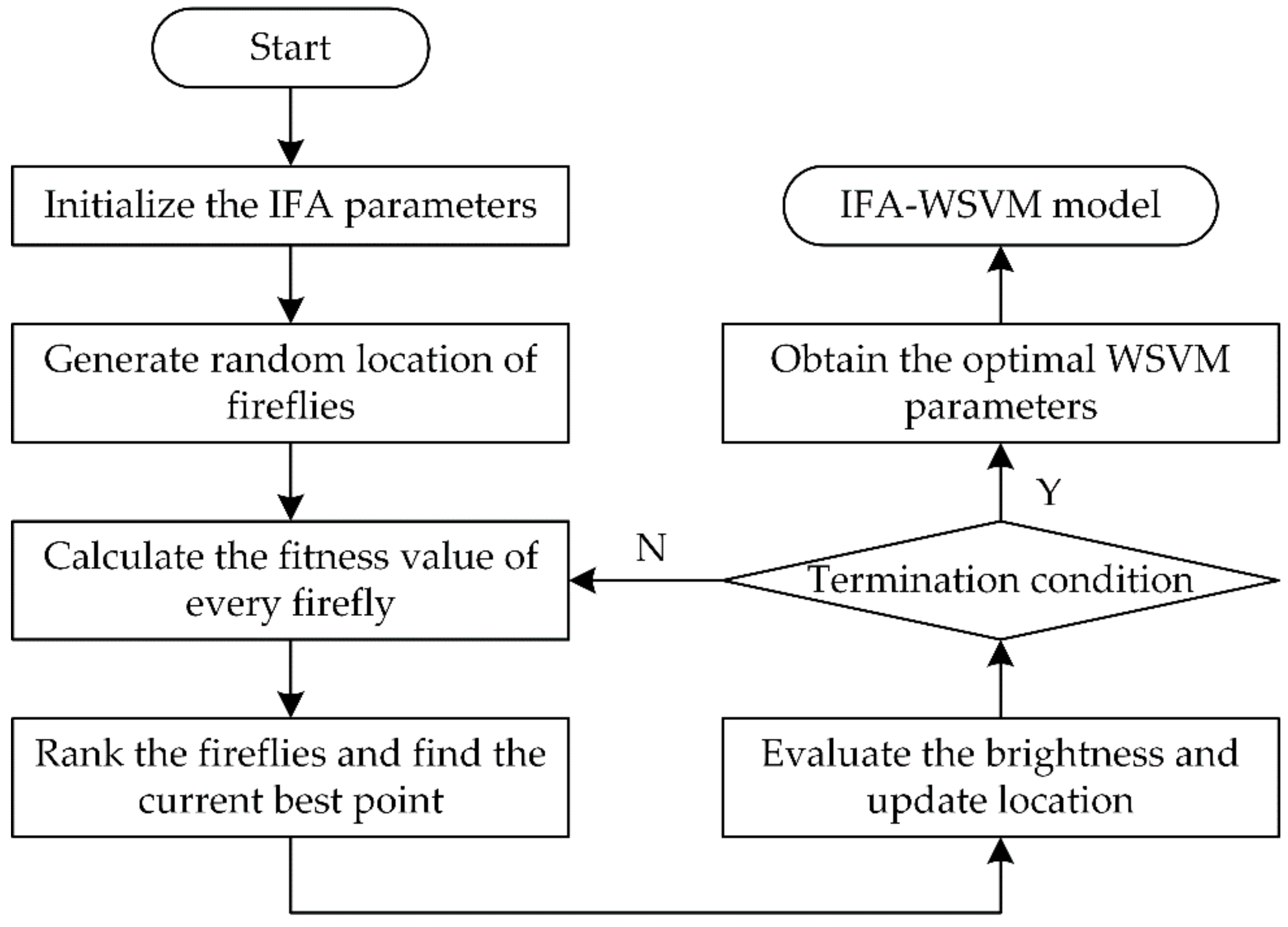
The procedure of IFA-WSVM model construction is illustrated in the flow diagram shown in Figure 1. Equally important, the process of optimizing WSVM parameters with IFA is also described as follows:

Step 1.

Initialize the improved firefly algorithm, and set up the parameters, including the number of fireflies $K$, initial and final randomization parameters ${\alpha }_0$ and ${\alpha }_{\infty }$, maximum iterations $t_{\max }$, attractiveness ${\beta }_0$, basic attractiveness ${\beta }_b$ and light absorption coefficient $\gamma$.

Step 2.

Generate the initial locations of fireflies at random as $x_i\left(i=1, 2, \cdots , K\right)$, every firefly is composed of the WSVM parameters $C$ and $\tau$.

Step 3.

Calculate the fitness value of every firefly to determine or update its brightness.

Step 4.

Rank the fireflies by their brightness and regard the firefly with minimum brightness as the global-best point.

Step 5.

Evaluate the brightness of every current firefly and compare the brightness of any two fireflies $i$ and $j$. If $I_i>I_j$, calculate the distance $r_{ij}$ to obtain the improved attractiveness $\tilde{\beta }\left(r_{ij}\right)$. Then, move firefly $i$ towards $j$ in all dimensions using Equation (28). The randomization parameter $\alpha \left(t+1\right)$ is updated by Equation (26).

Step 6.

Check termination condition. If the maximum iteration limit is reached, stop the optimization process and output the values of optimal parameters $C$ and $\tau$. Otherwise, return to Step 3.

4. Combustion State Recognition Based on IFA-WSVM Model

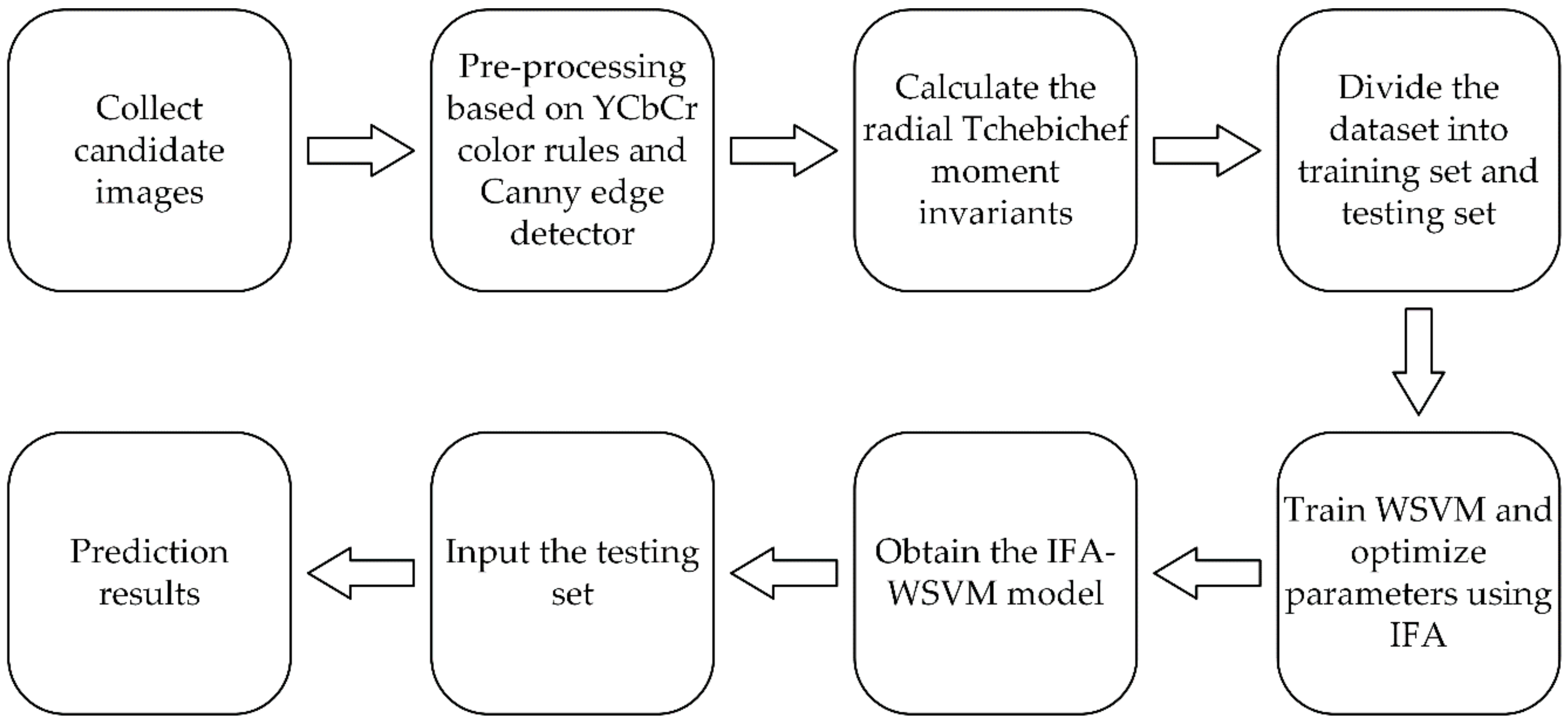
Based on the above contents, the method to recognize combustion state using IFA-WSVM model can be described step by step as follows:

Step 1.

Apply a video camera to collect a series of candidate images. Then, the pre-processed and edge images are obtained by pre-processing the candidate images.

Step 2.

Calculate the radial Chebyshev moment invariants of every pre-processed and edge image. Select the region and contour moment invariants to construct the corresponding feature vector $F_i$. The dataset is composed of all the feature vectors and their labels.

Step 3.

Divide the dataset into training set and testing set. The former is employed to construct model, and the latter is used for validating the IFA-WSVM model.

Step 4.

Train the WSVM with the feature vectors of training set, and apply IFA to determine the penalty factor $C$ and the dilation parameter $\tau$. When the termination condition is met, the optimal parameters are obtained.

Step 5.

Input the training data into the WSVM with optimal parameters once again, rebuilding the IFA-WSVM model. The features vectors of testing set are input into the IFA-WSVM model to predict their belonging labels, achieving the combustion state recognition.

Accordingly, the flow diagram of combustion state recognition based on the IFA-WSVM model is shown in Figure 2.

Furthermore, for the sake of evaluating the recognition performance of the IFA-WSVM model, the operating time and the recognition rate ($RRT$) are selected as the evaluation indexes. In general, the shorter operating time, the higher the work efficiency; the higher the value of $RRT$, the better the recognition performance of the model. The $RRT$ can be calculated by the following equation:

$$RRT=\frac{T_1+T_2\cdots +T_n}{Sum}\times 100\%$$

(30)

5. Case Studies

5.1. Study Setup

In our case studies, the candidate images were gathered by a video camera monitoring the burning fire for a period of time. An oil pan was utilized as the burner, which was about 570 mm in diameter. Five liters of normal heptane were poured into the oil pan as fuel for the fire. Considering the security, the fuel was additionally mixed with twelve liters of water. An aerosol fire extinguisher was used to put out the flames. In order to evaluate the generalization capabilities of the proposed method, the candidate images were acquired at different times and in several different conditions. Meanwhile, the position and orientation of the flame in the scene and the flame-to-camera distance were also adjusted. What’s more, some similar type of non-flame images were captured to test the robustness in handling false alarm sources. Finally, there were 3502 candidate images collected, with a size of $266 \times 236$.

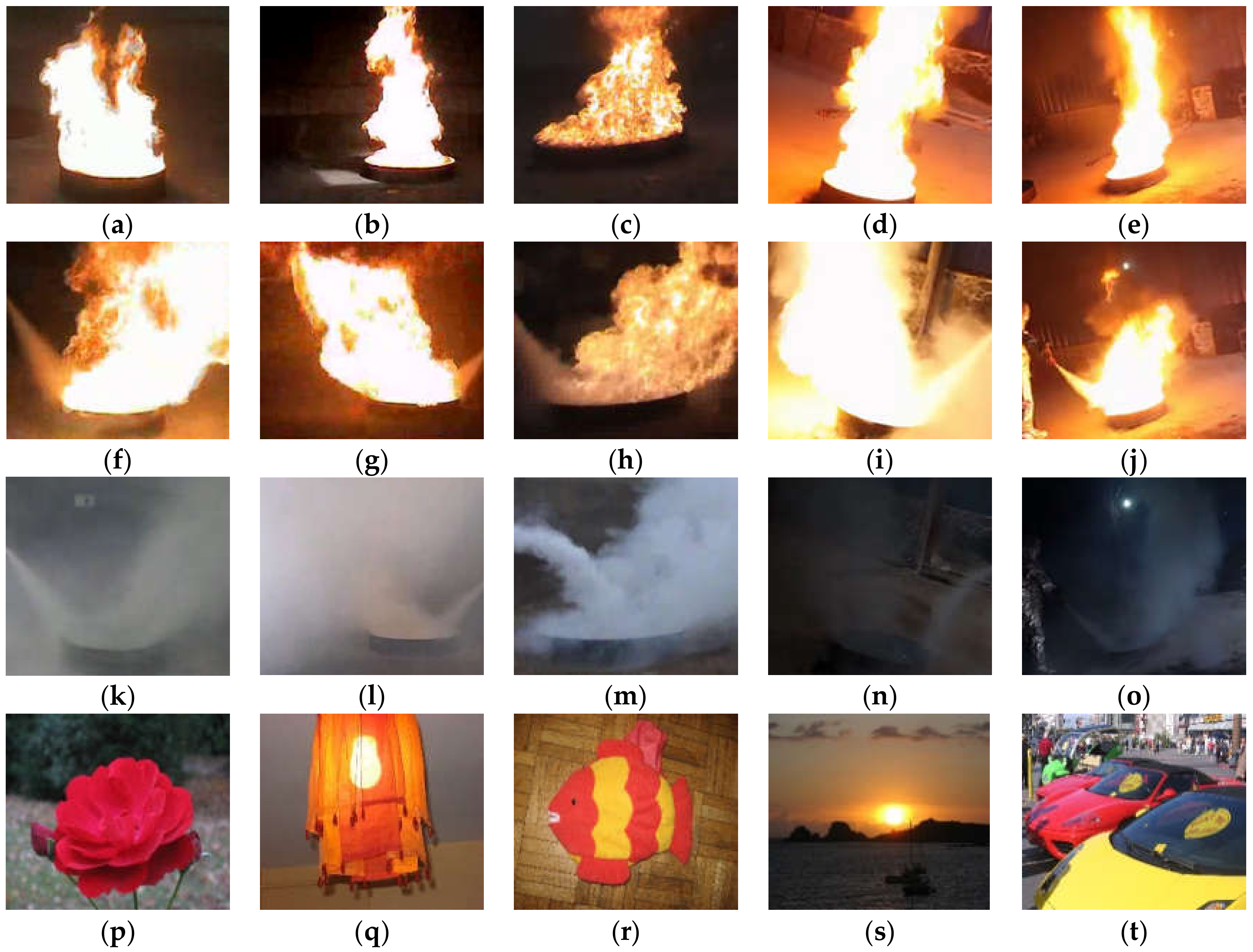
Among them, the 1st–2254th candidate images contained the flame burning steadily, as shown in Figure 3a–e; the 2255th–2779th candidate images exhibited the flame being extinguished by a fire extinguisher, as shown in Figure 3f–j; the 2780th–3194th candidate images showed the extinguished flame, as shown in Figure 3k–o; the 3195th–3502nd candidate images contained flame-color objects, such as red flowers, lighting, sunset, and so on. Here, the first 2254 images were classified as stable burning state, the next 525 images were classified as extinguishing state; the following 415 images were classified as final extinguished state; the last 308 images were classified as non-flame state. However, it can be observed that some images with an extinguishing state are quite similar to those with a stable burning state, which increases the difficulty of recognition.

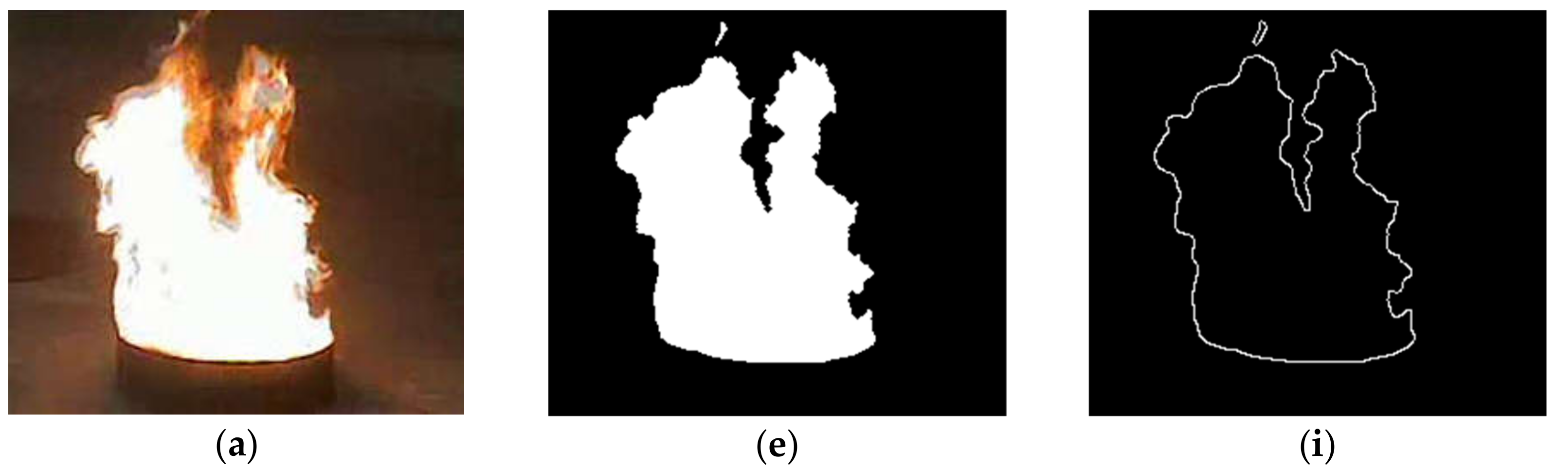
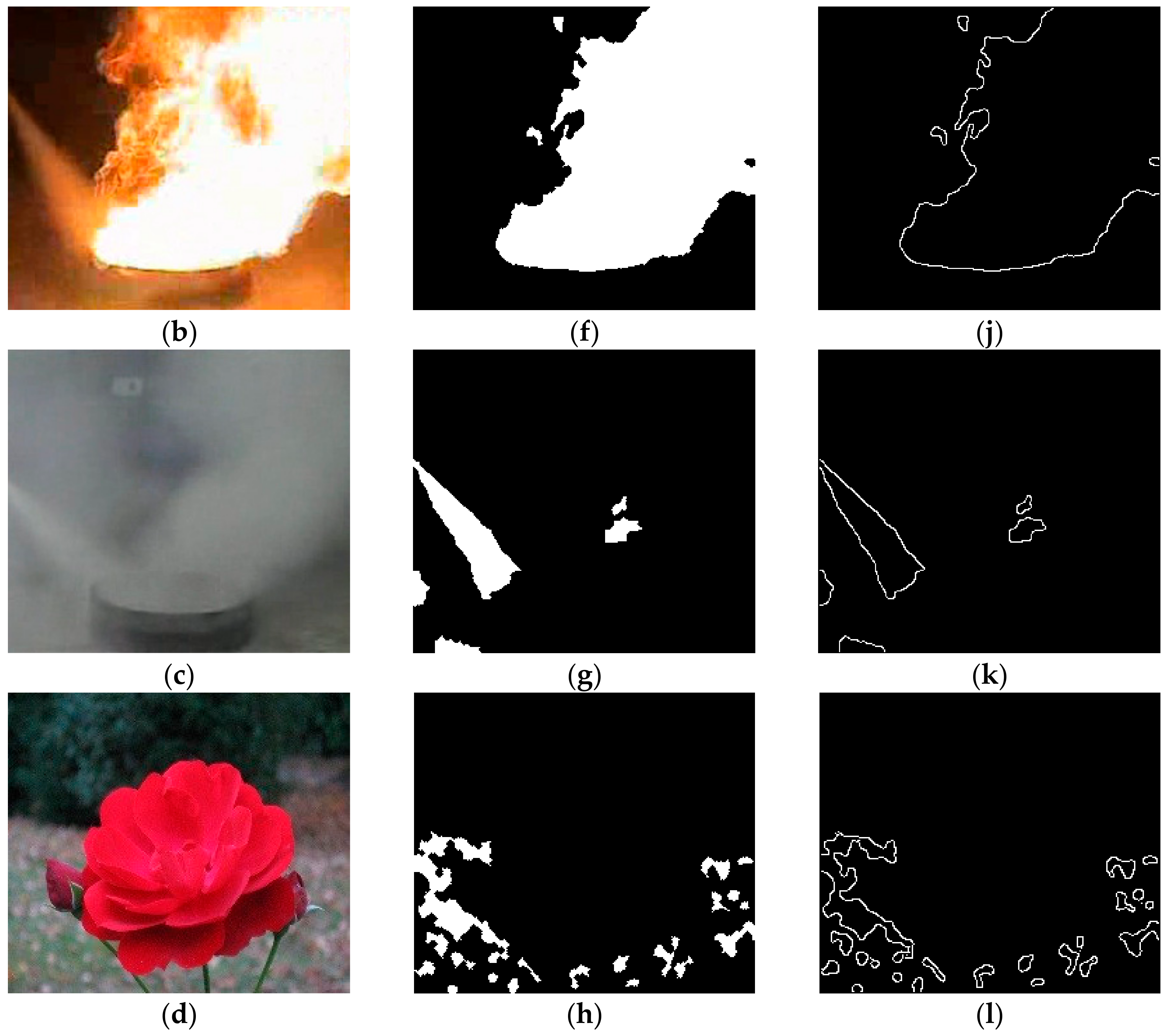
First of all, the candidate images were segmented with the proposed rules and converted into pre-processed images. In order to eliminate noise, the closing operation and hole filling operation were also performed. Then, the edge images were obtained by applying the Canny edge detector to extract the potential flame contour. To extract the local and global multi-features, the RCMIs of pre-processed images and edge images were calculated to construct feature vectors. Finally, the IFA-WSVM model was used to recognize the combustion state of flame. Figure 4 shows some pre-processed images and edge images in our case studies respectively.

From Figure 3 and Figure 4, it can be observed that the stable burning flame has an irregular shape, containing a relatively large number of sharp angles. On the contrary, the shape of extinguishing flame is more regular and smooth. Due to that the flame was extinguished completely or absent, the images with final extinguished state and non-flame state show something small with strange shape, which are quite different from others.

The basic idea of SVM is to separate two classes from each other. However, the combustion state recognition corresponds to a multi-class classification problem. A solution is to decompose the original multi-class problem into several binary sub-problems. One-against-one approach is one of the most suitable approaches for practical use. In the pairwise decomposition, $c\left(c-1\right)/2$ different binary classifiers are built, each of which separates one class from another ignoring all the other classes. In the end, each classifier casts one vote for its preferred class, and the final result is the class with the most votes. For SVM, the one-against-one approach generally performs better than other SVM-based multi-class classification algorithms [40,41]. Therefore, it is selected for the multi-class IFA-WSVM classifiers.

Considering the running time and recognition performance of the experimental confirmation, some RCMIs of proper orders are selected to construct the feature vector.

Table 1. Average values of the region moment invariants.

	${\tilde{\mathit{C}}}_{\mathbf{13}}^{\prime }$	${\tilde{\mathit{C}}}_{\mathbf{21}}^{\prime }$	${\tilde{\mathit{C}}}_{\mathbf{23}}^{\prime }$	${\tilde{\mathit{C}}}_{\mathbf{25}}^{\prime }$	${\tilde{\mathit{C}}}_{\mathbf{26}}^{\prime }$	${\tilde{\mathit{C}}}_{\mathbf{32}}^{\prime }$	${\tilde{\mathit{C}}}_{\mathbf{44}}^{\prime }$	${\tilde{\mathit{C}}}_{\mathbf{55}}^{\prime }$
Stable burning state	0.05764	0.1434	0.06644	0.07413	0.05933	0.1205	0.07037	0.05952
Extinguishing state	0.09043	0.1052	0.07653	0.06037	0.04384	0.1627	0.09681	0.04934
Final extinguished state	0.1105	0.1751	0.05140	0.04476	0.03403	0.06471	0.05474	0.1346
Non-flame state	0.1022	0.1882	0.2518	0.1948	0.2879	0.3698	0.2118	0.2461
Coefficient of variation	25.73%	24.18%	84.35%	73.34%	114.36%	74.18%	65.54%	74.19%

and

Table 2. Average values of the contour moment invariants.

	${\tilde{\mathit{C}}}_{\mathbf{13}}^{″}$	${\tilde{\mathit{C}}}_{\mathbf{21}}^{″}$	${\tilde{\mathit{C}}}_{\mathbf{23}}^{″}$	${\tilde{\mathit{C}}}_{\mathbf{25}}^{″}$	${\tilde{\mathit{C}}}_{\mathbf{26}}^{″}$	${\tilde{\mathit{C}}}_{\mathbf{32}}^{″}$	${\tilde{\mathit{C}}}_{\mathbf{44}}^{″}$	${\tilde{\mathit{C}}}_{\mathbf{55}}^{″}$
Stable burning state	0.2231	0.2069	0.2632	0.2318	0.2162	0.5859	0.3427	0.3169
Extinguishing state	0.2418	0.2789	0.3329	0.2783	0.2824	0.4407	0.4145	0.4081
Final extinguished state	0.5374	0.7651	0.2971	0.2147	0.3470	0.7293	0.4514	0.4533
Non-flame state	0.2017	0.4388	0.3742	0.2721	0.2329	0.5646	0.3281	0.4908
Coefficient of variation	52.63%	58.74%	15.04%	12.40%	21.78%	20.39%	15.25%	17.97%

represent the corresponding average values of region and contour moment invariants of different classes respectively.

Coefficient of variation (CV) is defined as the ratio of the standard deviation to the absolute value of mean, which is used to measure the difference between different classes. The larger the value, the easier recognition is to achieve. For different features, it is easy to find that the CV values of region moment invariants are different from those of contour moment invariants. In the case of some features, the CV values of region moment invariants are relatively small, whereas the corresponding values of contour moment invariants are quite large, forming a mutually complementary relationship. Based on the CV values, the multi-feature vector $F_i$ used in this paper is expressed as follows:

$$F_i=\left[{\tilde{C}}_{13}^{″}, {\tilde{C}}_{21}^{″}, {\tilde{C}}_{23}^{\prime }, {\tilde{C}}_{25}^{\prime }, {\tilde{C}}_{26}^{\prime }, {\tilde{C}}_{32}^{\prime }, {\tilde{C}}_{44}^{\prime }, {\tilde{C}}_{55}^{\prime }\right]$$

(31)

In the optimization phase, the initialization of IFA was set as follows: the number of fireflies $K=10$, initial and final randomization parameters ${\alpha }_0=0.5$ and ${\alpha }_{\infty }={10}^{-4}$, maximum iterations $t_{\max }=50$, attractiveness ${\beta }_0=1$, basic attractiveness ${\beta }_b=0.2$ and light absorption coefficient $\gamma =1$. The WSVM parameters of $C$ and $\tau$ for the wavelet kernel function were varied in the fixed range of $\left[0.01, 100\right]$. The above initialization parameters are given in

Table 3. The initialization parameters of IFA.

Parameter	Value	Range	Description
$K$	10	—	Number of fireflies
${\alpha }_0$	0.5	—	Initial randomization parameters
${\alpha }_{\infty }$	${10}^{-4}$	—	Final randomization parameters
$t_{\max }$	50	—	Maximum number of iterations
${\beta }_0$	1	—	Attractiveness
${\beta }_b$	0.2	—	Basic attractiveness
$\gamma$	1	—	Light absorption coefficient
$C$	—	$[0.01, 100]$	Penalty factor of WSVM
$\tau$	—	$[0.01, 100]$	Dilation parameter of WSVM

. All the case studies were developed under the MATLAB 2016b programming environment, and performed on a personal computer with Intel(R) Core(TM) i7 CPU 4GHz, 16G memory, whose operation system is Microsoft Windows 7 Ultimate.

5.2. Results and Discussion

5.2.1. Results for the First Case Study and Comparison

In the first case study, 1009 images with a stable burning state, 235 images with an extinguishing state, 186 images with a final extinguished state, and 138 images with a non-flame state were randomly selected as the training set to construct the IFA-WSVM model. The rest of candidate images were regarded as the testing set to validate the model performance. Depending on Equation (31), the multi-feature vectors were formed by calculating the RCMIs of the pre-processed images and edge images. Then, the training set was input into the WSVM, and the best values of the WSVM parameters were sought by the IFA algorithm. Here, the optimal parameters were generated as follows: $C=63.2396$, $\tau =9.7631$. Next, the multi-feature vectors of the training set were input into the WSVM with the optimal parameters again, obtaining the IFA-WSVM model. In the end, the training set was input into the IFA-WSVM model to recognize the combustion state. In order to evaluate the performance of the proposed method, the comparison of the methods based on HMIs, ZMIs and RCMIs was performed. What’s more, a comparison with the methods based on multi-features and region moment invariants was also carried out. The results of the first case study are shown in

Table 4. Recognition results of the testing set in the first case study.

Parameter	Region Moments			Region and Contour Moments
	Hu	Zernike	Radial-Chebyshev	Hu	Zernike	Radial-Chebyshev
Recognition amount	1751	1808	1875	1796	1844	1916
Recognition rate	90.54%	93.49%	96.95%	92.86%	95.35%	99.07%
Average operating time of a single image	32.19 ms	103.54 ms	41.07 ms	66.16 ms	205.79 ms	83.38 ms

.

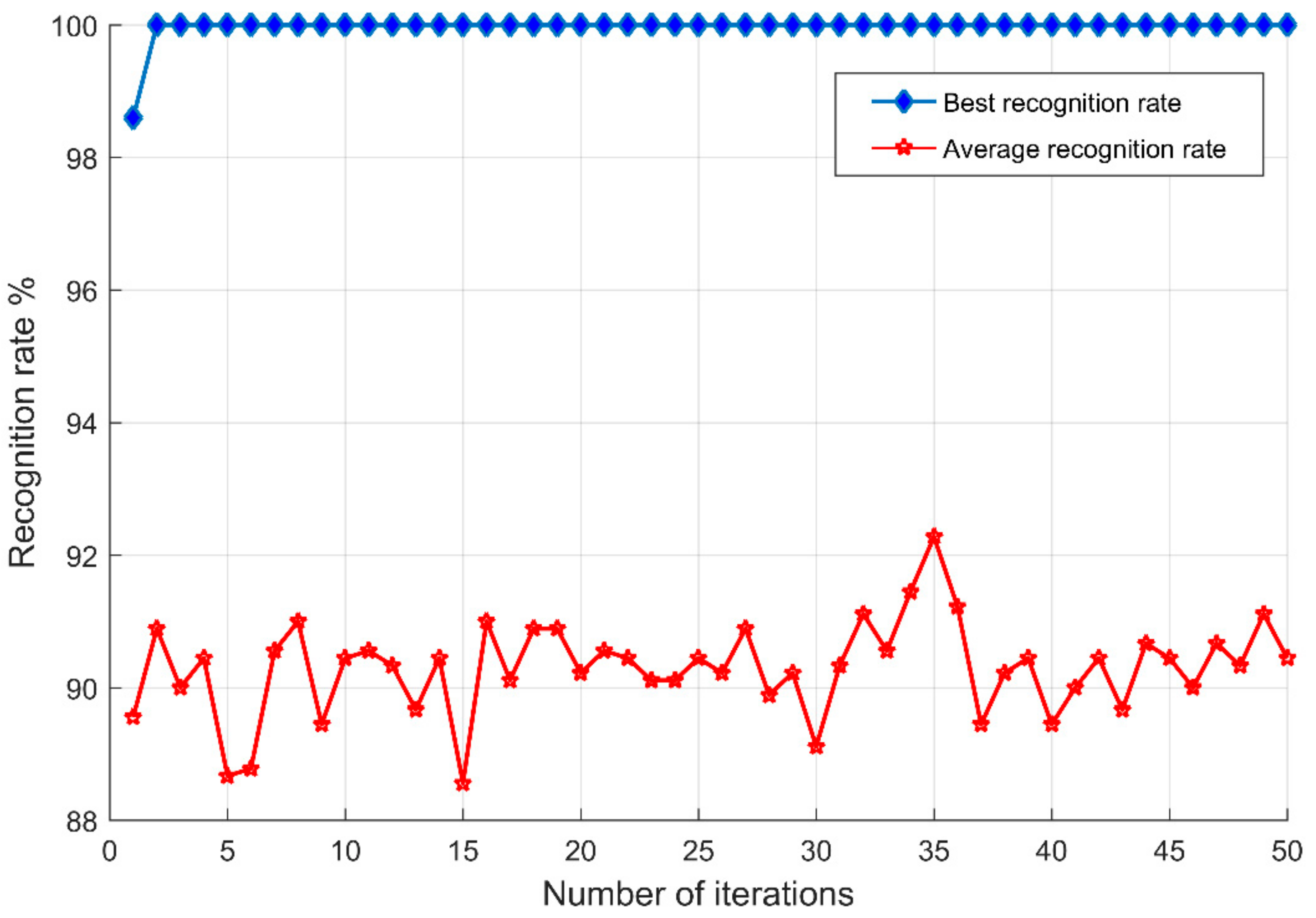
From Table 4, it can be observed that the HMIs derived from non-orthogonal polynomials achieve the lowest recognition rate of 90.54%. RCMIs can achieve better accuracy of recognition than HMIs and ZMIs. In addition, the multi-feature vectors, formed by combining region moment invariants with contour moment invariants, can improve the recognition rate significantly, achieving the highest recognition of 99.07%. In terms of operating time, the work efficiency of RCMIs is apparently higher than that of ZMIs. Although a little lower than HMIs, the methods based on RCMIs can still satisfy the requirement of real-time. However, it also should be noted that the images used are in low definition, with a size of $266 \times 236$. This is one of the reasons for achieving a low time processing. As shown in Figure 5, the effectiveness of IFA-WSVM model was also confirmed by the fact that it achieved the highest rate of recognition during the optimization phase.

5.2.2. Results for the Second Case Study and Comparison

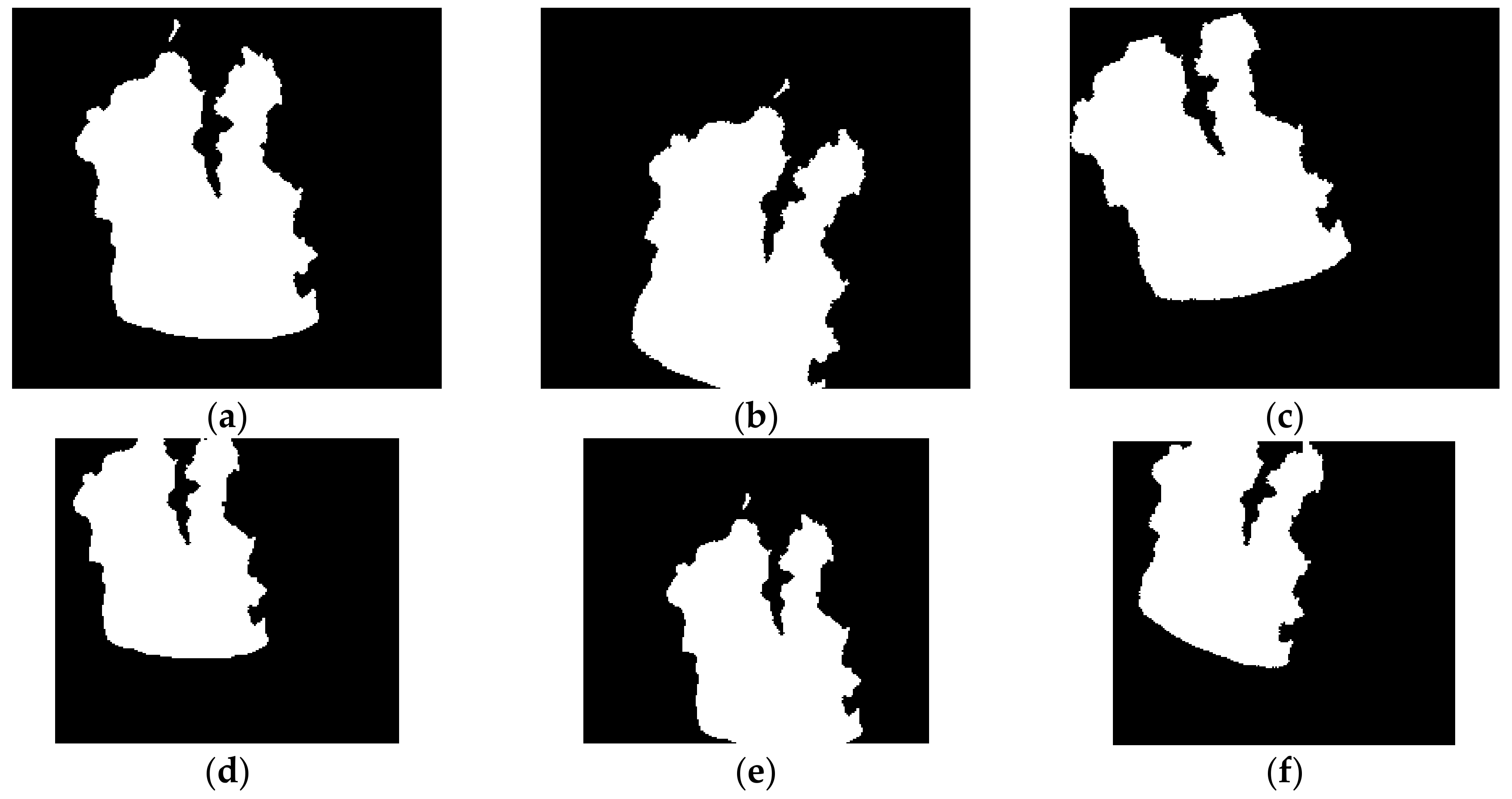
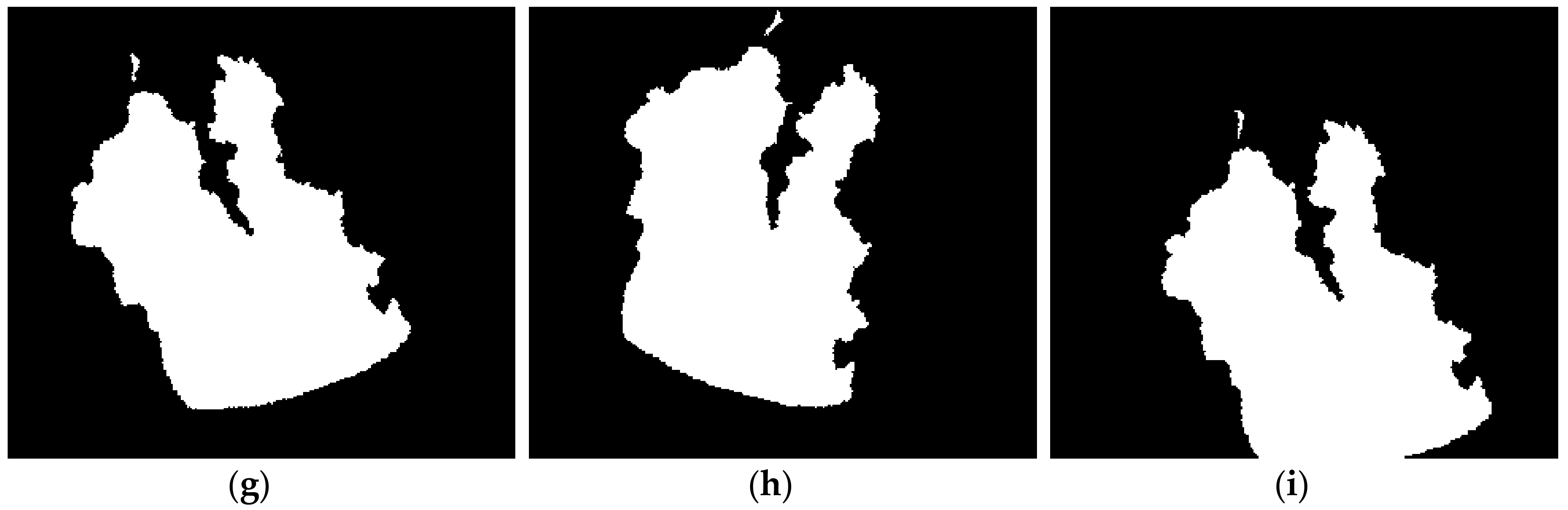
The aim of the second case study is to illustrate the performance of the proposed method in the RTS transformation set. First, two images of each state were selected as the temporary set. Then, each image of temporary set was rotated by angels $\pm {15}^{\circ }$ and $\pm {20}^{\circ }$, translated with translation vectors $\left[-35, -25\right]$ and $\left[35, 25\right]$, scaled with scaling factors of 0.5, 0.8, 1.2 and 1.5. Consequently, a RTS transformation set was obtained including 600 ($8\times 75$) images. Some of their pre-processed images are illustrated in Figure 6. Accordingly, their values of radial Chebyshev moment invariants are given in

Table 5. Radial Chebyshev moment invariants of the images in Figure 6.

	${\tilde{\mathit{C}}}_{\mathbf{13}}^{\prime }$	${\tilde{\mathit{C}}}_{\mathbf{21}}^{\prime }$	${\tilde{\mathit{C}}}_{\mathbf{23}}^{\prime }$	${\tilde{\mathit{C}}}_{\mathbf{25}}^{\prime }$	${\tilde{\mathit{C}}}_{\mathbf{26}}^{\prime }$	${\tilde{\mathit{C}}}_{\mathbf{32}}^{\prime }$	${\tilde{\mathit{C}}}_{\mathbf{44}}^{\prime }$	${\tilde{\mathit{C}}}_{\mathbf{55}}^{\prime }$
(a)	0.05444	0.07434	0.04488	0.03860	0.07514	0.2510	0.08892	0.07073
(b)	0.06002	0.07957	0.04718	0.03732	0.07636	0.2244	0.08912	0.07578
(c)	0.05684	0.07554	0.04697	0.03652	0.07114	0.2494	0.09563	0.06927
(d)	0.05888	0.07493	0.04831	0.03963	0.08176	0.2232	0.09072	0.07867
(e)	0.05713	0.07609	0.04288	0.03778	0.07301	0.2431	0.08103	0.07241
(f)	0.05563	0.07076	0.04622	0.03576	0.07406	0.2499	0.08882	0.07744
(g)	0.05484	0.07380	0.04410	0.03947	0.07741	0.2507	0.09012	0.07114
(h)	0.05863	0.07114	0.04512	0.03465	0.07286	0.2206	0.09840	0.07812
(i)	0.05261	0.07264	0.04923	0.04097	0.08093	0.2646	0.08392	0.08116
Coefficient of variation	4.24%	3.64%	4.43%	5.34%	4.81%	6.39%	5.88%	5.59%

. It can be observed that the proposed multi-feature vectors are really invariant to rotation, translation and scaling.

Among the 75 images of each sample of temporary set, 20 images were randomly selected as the training set. There were 160 images in the training set, and the remaining 440 images were used as the testing set. In the same way, after the pre-processing, the methods based on HMIs, ZMIs and RCMIs were used to extract the local and global multi-features, and the IFA-WSVM model was utilized to recognize the combustion state. Due to the randomness, the best results obtained by the proposed algorithms are given in

Table 6. Recognition results of the testing set in the second case study.

Parameter	Region Moments			Region and Contour Moments
	Hu	Zernike	Radial-Chebyshev	Hu	Zernike	Radial-Chebyshev
Recognition amount	376	391	419	397	412	433
Recognition rate	85.45%	88.86%	95.23%	90.23%	93.64%	98.41%
Average operating time of a single image	33.39 ms	100.90 ms	46.37 ms	67.84 ms	198.16 ms	90.42 ms

.

As seen from the results for second case study, the global region moment invariants alone cannot get a good effect of recognition. On the contrary, the combination of region moment invariants and contour moment invariants contributes to achieving the higher recognition rates. Among these methods, the method based on RCMIs can still have the highest recognition rate. Besides this, the operating time further confirms the viability of real-time recognition herein, saving a lot of computational resources.

5.2.3. Results for the Third Case Study and Comparison

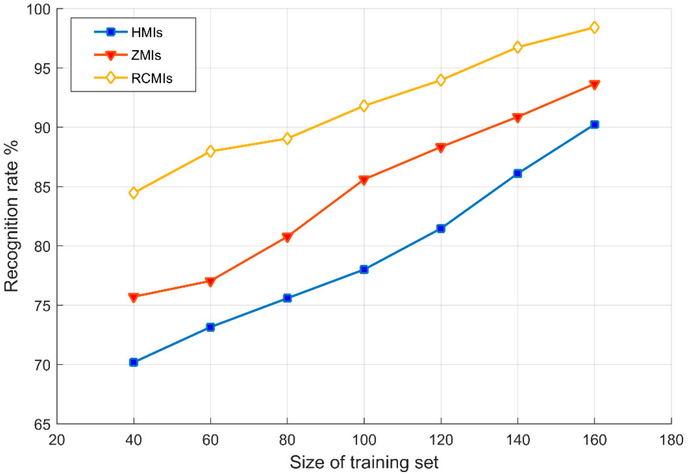
In the third case study, the effect of changing in size of training set on the recognition rate was observed. There were 10, 15, 20, 25, 30, 35 and 40 images of each state randomly selected from the RTS transformation set as the training sets. Accordingly, the rest of images transformed by RTS composed seven corresponding testing sets. Similarly, a comparison of the methods based on RCMIs, HMIs and ZMIs was also performed in the third case study. The result for the third case study can be observed in Figure 7.

According to Figure 7, it can be found that all the recognition rates reach their respective lowest points at the beginning. This is explained by the fact that the size of training set is so small that the description of images is not accurate. However, as the size of training set increases, the rate of recognition puts forward a rising tendency. In the end, all the recognition rates get to their respective maximum. Furthermore, when the size of training set is 40, the recognition rates of the methods based on HMIs and ZMIs are only 70.18% and 75.71% respectively. However, the method based on RCMIs can still achieve a recognition rate of 84.46% at this point. Besides, in the process of increasing the size, the fluctuation in the recognition rate of the method using RCMIs is smallest among these methods, showing that its stability is the best.

5.2.4. Results for the Fourth Case Study and Comparison

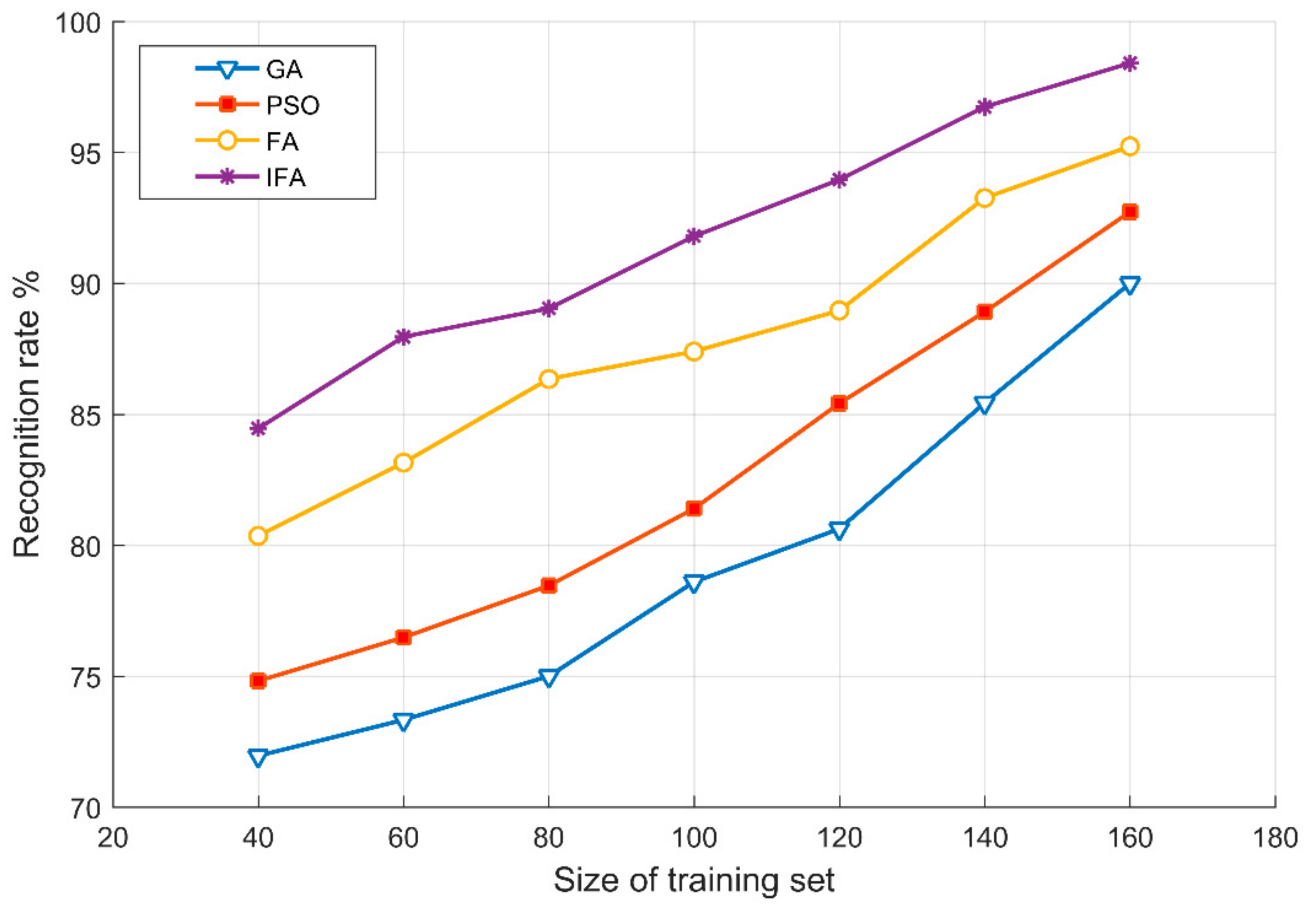
To illustrate the performance of IFA, the comparison of IFA with FA, GA and PSO was performed. Here, the training sets and testing sets used in the second case study were applied again. The difference is that only the method based on RCMIs was implemented. Results obtained by IFA and other methods in the fourth case study are presented in Figure 8.

Compared with other models, it can be obviously observed that the GA-WSVM model has the worst performance. The curve of GA-WSVM model is very large, ranging from 71.96% to 90.00%, and it has the lowest point. PSO-WSVM and FA-WSVM models have a good performance, but their curves are still relatively large, ranging from 74.82% to 92.73% and 80.36% to 95.23% respectively. Whereas the IFA-WSVM model has a better performance and outperforms other models, whose curve tends to more gentle and has the highest recognition rate throughout the different experiments. In conclusion, the results indicate that the proposed IFA-WSVM model presents better performance in state recognition than the other three methods, even when the size of the training set is small.

5.2.5. Discussion

As for the first three case studies, it is worth pointing out that the features extracted by Hu moments contain redundant information, and the ability of image description is not strong enough that the recognition rate is very low. Zernike moments with orthogonal polynomial basis can reconstruct the original image using a limited set of moments, having a great capability of describing the object. However, they are in the continuous domain of image coordinate space. The continuous integral is approximated by a discrete summation in the calculation, involving some numerical approximations. In contrast, the Chebyshev polynomials are discrete orthogonal polynomials, overcoming the deficiency of Hu moments and Zernike moments in terms of object representation and calculation. Thus, they can present the best performance of image description.

In addition, the moments derived from the edge images contain more information about the high-frequency portions than those derived from the pre-processed images. As a result, the minute details of the images, such as the sharp angles of the flame, are better characterized by the contour moments. On the other hand, the global features of the flame can be better characterized by the region moments. Besides, these moments are less sensitive to noise. Hence, these advantages make the combination of region with contour moments superior to the region moments, improving the accuracy of feature extraction.

With regard to the fourth case study, the reason for this result is that the GA method has the defects of earlier maturity and slow convergent in the later stage of evolution. So that it is not in a position to find the global optimal solution. Similarly, in the convergence of PSO method, the adjustment of each particle’s velocity and position is over depend on the current optimal particle, leading to produce premature convergence and fall into the local optimal solution. However, due to the comparison of any two fireflies, the image information is exchanged more adequately and effectively in the FA and IFA method, which contributes to skipping the local optimal and achieve the global optimal.

Moreover, due to the improved attractiveness, the worse solutions can move towards the better ones, improving the convergence rate. Using the modified randomization parameter, the proposed location update of IFA is able to adjust its searching step dynamically according to the situation of iterations, improving the recognition rate of the method finally.

From the above discussion, the conclusion can be reached that the proposed method based on RCMIs and IFA-WSVM model can achieve combustion state recognition effectively and accurately, which has been proven to be superior to methods based on HMIs and ZMIs. The proposed IFA-WSVM model has advantages over other models based on GA, PSO and FA, which can be considered as an effective classification method for combustion state recognition.

6. Conclusions

In this paper, a novel and effective method for combustion state recognition of flame images based on RCMIs and IFA-WSVM model is proposed. The candidate images are pre-processed by YCbCr color rules and Canny edge detectors. Then, the RCMIs of pre-processed and edge images are applied to construct the multi-feature vectors, which improves the accuracy of feature extraction. To break away from the local optimum, an improved FA algorithm is developed. Then, an IFA-WSVM model is built with the feature vectors of the training set, to which the IFA is used to optimize the penalty factor and dilation parameter of WSVM. Finally, the results for case studies demonstrate that the proposed method is superior to other methods and achieves the highest rate, up to 99.07%. The proposed IFA algorithm also outperforms other benchmark algorithms, including GA, PSO and FA. The methods based on multi-features improve the accuracy of feature extraction, making them superior to those based on region moment invariants. They can also satisfy the requirement of real-time recognition, saving a lot of computational resources. It is also worth pointing out that the images used are in low definition, which contributes to achieving a low time processing and real-time recognition. What’s more, even if the images are transformed by RTS and the size of training set is small, the method based on RCMIs and IFA-WSVM model continues to exhibit the best performance, which may have implications and wide application in the combustion state recognition of flame images.

References

- Duong, H.D.; Tinh, D.T. An efficient method for vision-based fire detection using SVM classification. In Proceedings of the International Conference on Soft Computing and Pattern Recognition (SoCPaR), Hanoi, Vietnam, 15–18 December 2013. [Google Scholar]
- Hasan, M.M.; Razzak, M.A. An automatic fire detection and warning system under home video surveillance. In Proceedings of the IEEE 12th International Colloquium on Signal Processing & ITS Applications (CSPA), Malacca, Malaysia, 4–6 March 2016. [Google Scholar]
- Jayashree, D.; Pavithra, S.; Vaishali, G.; Vidhya, J. System to detect fire under surveillanced area. In Proceedings of the Third International Conference on Science Technology Engineering & Management (ICONSTEM), Chennai, India, 23–24 March 2017. [Google Scholar]
- Lascio, R.D.; Greco, A.; Saggese, A.; Vento, M. Improving fire detection reliability by a combination of videoanalytics. In Proceedings of the 11th International Conference on Image Analysis and Recognition (ICIAR), Vilamoura, Portugal, 22–24 October 2014. [Google Scholar]
- Zhang, Z.J.; Shen, T.; Zou, J.H. An Improved Probabilistic Approach for Fire Detection in Videos. Fire Technol. 2014, 50, 745–752. [Google Scholar] [CrossRef]
- Duong, H.D.; Tinh, D.T. A new approach to vision-based fire detection using statistical features and Bayes classifier. In Proceedings of the 9th International Conference on Simulated Evolution and Learning (SEAL), Hanoi, Vietnam, 16–19 December 2012. [Google Scholar]
- Shao, L.S.; Guo, Y.C. Flame recognition algorithm based on Codebook in video. J. Comput. Appl. 2015, 35, 1483–1487. [Google Scholar]
- Sandhu, H.S.; Singh, K.J.; Kapoor, D.S. Automatic edge detection algorithm and area calculation for flame and fire images. In Proceedings of the 6th International Conference-Cloud System and Big Data Engineering (Confluence), Noida, India, 14–15 January 2016. [Google Scholar]
- Wang, Y.K.; Wu, A.G.; Zhang, J.; Zhao, M.; Li, W.S.; Dong, N. Fire smoke detection based on texture features and optical flow vector of contour. In Proceedings of the 12th World Congress on Intelligent Control and Automation (WCICA), Guilin, China, 12–15 June 2016. [Google Scholar]
- Maksymiv, O.; Rak, T.; Peleshko, D. Real-time fire detection method combining AdaBoost, LBP and convolutional neural network in video sequence. In Proceedings of the 14th International Conference the Experience of Designing and Application of Cad Systems in Microelectronics (CADSM), Lviv, Ukraine, 21–25 February 2017. [Google Scholar]
- Russo, A.U.; Deb, K.; Tista, S.C.; Islam, A. Smoke Detection Method Based on LBP and SVM from Surveillance Camera. In Proceedings of the International Conference on Computer, Communication, Chemical, Material and Electronic Engineering (IC4ME2), Rajshahi, Bangladesh, 8–9 February 2018. [Google Scholar]
- Wang, D.; Cui, X.N.; Park, E.; Jin, C.L.; Kim, H. Adaptive flame detection using randomness testing and robust features. Fire Saf. J. 2013, 55, 116–125. [Google Scholar] [CrossRef]
- Zhong, Z.; Wang, M.J.; Shi, Y.K.; Gao, W.L. A convolutional neural network-based flame detection method in video sequence. Signal Image Video Process. 2018, 12, 1619–1627. [Google Scholar] [CrossRef]
- Lin, Y.J.; Chai, L.; Zhang, J.X.; Zhou, X.J. On-line burning state recognition for sintering process using SSIM index of flame images. In Proceedings of the 11th World Congress on Intelligent Control and Automation, Shenyang, China, 29 June–4 July 2014. [Google Scholar]
- Cheng, Y.; Sheng, Y.X.; Chai, L. Burning state recognition using CW-SSIM index evaluation of color flame images. In Proceedings of the 27th Chinese Control and Decision Conference (CCDC), Qingdao, China, 23–25 May 2015. [Google Scholar]
- Prema, C.E.; Vinsley, S.S.; Suresh, S. Multi Feature Analysis of Smoke in YUV Color Space for Early Forest Fire Detection. Fire Technol. 2016, 52, 1–24. [Google Scholar]
- Shi, L.F.; Long, F.; Zhan, Y.J.; Lin, C.H. Video-based fire detection with spatio-temporal SURF and color features. In Proceedings of the 12th World Congress on Intelligent Control and Automation (WCICA), Guilin, China, 12–15 June 2016. [Google Scholar]
- Yan, X.F.; Cheng, H.; Zhao, Y.D.; Yu, W.H.; Huang, H.; Zheng, X.L. Real-Time Identification of Smoldering and Flaming Combustion Phases in Forest Using a Wireless Sensor Network-Based Multi-Sensor System and Artificial Neural Network. Sensors 2016, 16, 1228. [Google Scholar] [CrossRef] [PubMed]
- Chauhan, A.; Semwal, S.; Chawhan, R. Artificial neural network-based forest fire detection system using wireless sensor network. In Proceedings of the Annual IEEE India Conference (INDICON), Mumbai, India, 13–15 December 2013. [Google Scholar]
- Ghorbani, M.A.; Shamshirband, S.; Zare Haghi, D.; Azani, A.; Bonakdari, H.; Ebtehaj, I. Application of firefly algorithm-based support vector machines for prediction of field capacity and permanent wilting point. Soil Tillage Res. 2017, 172, 32–38. [Google Scholar] [CrossRef]
- Vapnik, V. The Nature of Statistical Learning Theory, 2nd ed.; Springer: New York, NY, USA, 1999. [Google Scholar]
- Niu, X.; Yang, C.; Wang, H.; Wang, Y. Investigation of ANN and SVM based on limited samples for performance and emissions prediction of CRDI-assisted marine diesel engine. Appl. Ther. Eng. 2016, 111, 1353–1364. [Google Scholar] [CrossRef]
- Sung, A.H.; Mukkamala, S. Identifying important features for intrusion detection using support vector machines and neural networks. In Proceedings of the Symposium on Applications and the Internet, Orlando, FL, USA, 27–31 January 2003. [Google Scholar]
- Motamedi, S.; Shamshirband, S.; Ch, S.; Hashim, R.; Arif, M. Soft computing approaches for forecasting reference evapotranspiration. Comput. Electron. Agric. 2015, 113, 164–173. [Google Scholar]
- Jiang, M.L.; Jiang, L.; Jiang, D.D.; Xiong, J.P.; Shen, J.G.; Ahmed, H.S.; Luo, J.Y.; Song, H.B. Dynamic Measurement Errors Prediction for Sensors Based on Firefly Algorithm Optimize Support Vector Machine. Sustain. Cities Soc. 2017, 35, 250–256. [Google Scholar] [CrossRef]
- Li, Y.F.; Chen, M.N.; Lu, X.D.; Zhao, W.Z. Research on optimized GA-SVM vehicle speed prediction model based on driver-vehicle-road-traffic system. Sci. China Technol. Sci. 2018, 61, 782–790. [Google Scholar] [CrossRef]
- Liu, X.; Gang, C.; Gao, W.; Zhang, K. GA-AdaBoostSVM classifier empowered wireless network diagnosis. Eurasip J. Wirel. Commun. Netw. 2018, 77, 1–18. [Google Scholar] [CrossRef]
- Ding, S.; Hang, J.; Wei, B.; Wang, Q. Modelling of supercapacitors based on SVM and PSO algorithms. IET Electr. Power Appl. 2018, 12, 502–507. [Google Scholar] [CrossRef]
- Ma, Z.; Dong, Y.; Liu, H.; Shao, X.; Wang, C. Method of Forecasting Non-Equal Interval Track Irregularity Based on Improved Grey Model and PSO-SVM. IEEE Access. 2018, 6, 34812–34818. [Google Scholar] [CrossRef]
- Yang, X.S. Firefly Algorithm, Stochastic Test Functions and Design Optimisation. Int. J. Bio-Inspired Comput. 2010, 2, 78–84. [Google Scholar] [CrossRef]
- Celik, T.; Ozkaramanlt, H.; Demirel, H. Fire Pixel Classification using Fuzzy Logic and Statistical Color Model. In Proceedings of the IEEE International Conference on Acoustics, Speech and Signal Processing, Honolulu, HI, USA, 15–20 April 2007. [Google Scholar]
- Jia, Y.; Wang, H.; Yan, H.U.; Dang, B. Flame detection algorithm based on improved hierarchical cluster and support vector machines. Comput. Eng. Appl. 2014, 50, 165–168. [Google Scholar]
- BT. 601: Studio Encoding Parameters of Digital Television for Standard 4:3 and Wide Screen 16:9 Aspect Ratios. Available online: https://www.itu.int/rec/R-REC-BT.601-7-201103-I/en (accessed on 1 November 2018).
- Canny, J. A Computational Approach to Edge Detection. IEEE Trans. Pattern Anal. Mach. Intell. 1986, 8, 679–698. [Google Scholar] [CrossRef] [PubMed]
- Flusser, J.; Zitova, B.; Suk, T. Moments and Moment Invariants in Pattern Recognition, 1st ed.; Wiley & Sons Ltd.: West Sussex, UK, 2009. [Google Scholar]
- Nikiforov, A.F.; Uvarov, V.B.; Suslov, S.K. Classical Orthogonal Polynomials of a Discrete Variable; Springer: New York, NY, USA, 1991. [Google Scholar]
- Mukundan, R. Radial Tchebichef Invariants for Pattern Recognition. In Proceedings of the Tencon 2005 IEEE Region 10 Conference, Melbourne, Australia, 21–24 November 2005. [Google Scholar]
- Zhong, W.; Zhuang, Y.; Sun, J.; Gu, J.J. A load prediction model for cloud computing using PSO-based weighted wavelet support vector machine. Appl. Intell. 2018, 48, 4072–4083. [Google Scholar] [CrossRef]
- Du, P.; Tan, K.; Xing, X. Wavelet SVM in Reproducing Kernel Hilbert Space for hyperspectral remote sensing image classification. Opt. Commun. 2010, 283, 4978–4984. [Google Scholar] [CrossRef]
- Kang, S.; Cho, S.; Kang, P. Constructing a multi-class classifier using one-against-one approach with different binary classifiers. Neurocomputing 2015, 149, 677–682. [Google Scholar] [CrossRef]
- Galar, M.; Ndez, A.; Barrenechea, E.; Bustince, H.; Herrera, F. An overview of ensemble methods for binary classifiers in multi-class problems: Experimental study on one-vs-one and one-vs-all schemes. Pattern Recognit. 2011, 44, 1761–1776. [Google Scholar] [CrossRef]
Figure 1.
The flow diagram of IFA-WSVM model construction
Figure 2.
The flow diagram of combustion state recognition based on IFA-WSVM model.
Figure 3.
Candidate images: (a–e) stable burning state; (f–j) extinguishing state; (k–o) final extinguished state; (p–t) non-flame state.
Figure 4.
Results of pre-processing: (a–d) original images; (e–h) pre-processed images; (i–l) edge images.
Figure 5.
The recognition rate curve of IFA-WSVM model.
Figure 6.
Pre-processed images of RTS transformation set. (a) Original image; (b) image rotated by −20° and translated with [35, 25]; (c) image rotated by 15° and translated with [−35, −25]; (d) image translated with [−35, −25] and scaled with 0.8; (e) image translated with [35, 25] and scaled with 0.8; (f) image rotated by −20° and scaled with 0.8; (g) image rotated by 20° and scaled with 1.2; (h) image rotated by −15° and scaled with 1.2; (i) image rotated by 15°, translated with [35, 25] and scaled with 1.2.
Figure 7.
Effect of changing in size of training set in the third case study.
Figure 8.
Comparison of the IFA with other methods in the fourth case study.