Hybrid Models Combining Technical and Fractal Analysis with ANN for Short-Term Prediction of Close Values on the Warsaw Stock Exchange

Abstract

This paper presents new methods and models for forecasting stock prices and computing hybrid models, combining analytical and neural approaches. First, technical and fractal analyses are conducted and selected stock market indices calculated, such as moving averages and oscillators. Next, on the basis of these indices, an artificial neural network (ANN) provides predictions one day ahead of the closing prices of the assets. New technical analysis indicators using fractal modeling are also proposed. Three kinds of hybrid model with different degrees of fractal analysis were considered. The new hybrid modeling approach was compared to previous ANN-based prediction methods. The results showed that the hybrid model with fractal analysis outperforms other models and is more robust over longer periods of time.

1. Introduction

Information about the current conditions on the Stock Exchange and future closing prices is crucial for investors, who wish to maximize their profits and make good investment decisions. Over the years, different theories and stock models have been developed, some of which contradicted each other. Until the second half of twentieth century, it was believed that price changes were random and thus could not be predicted. This was a basic assumption of the random walk hypothesis [1], which is consistent with the efficient market hypothesis (EMH) formulated by Eugene Fama [2]. This hypothesis states that share prices fully reflect all the available information, and stocks always trade at a fair value. It is therefore impossible to outperform the market overall, and higher returns can be only obtained by chance or by purchasing riskier investments. This hypothesis was not in line with experience, as evidenced by the profits amassed by professional financial institutions trading on stock markets. It was also refuted by a large group of academics, who observed and analyzed market prices over long periods of time and proved that market prices were not random, but exhibited trends [3,4]. Moreover, these trends repeated over time and some followed a sinusoidal shape [5]. These results supported the view that the market is, to some degree, predictable, and that future prices and trends can be predicted on the basis of past prices. This opened the way for technical analysis. Thus, the problem of stock price prediction is closely related to time series analysis and modeling trends.

These days, not only spectral analysis of trade signals [5], but also other more complex methods, such as joint time–frequency–shape analysis, are available [6].

The financial market provides a variety of software products supporting investors. Traditional prediction algorithms, such as autoregressive integrated moving average (ARIMA) and generalized autoregressive conditional heteroscedasticity (GARCH), are based on financial time series modeling using the stochastic process theory [7]. A linear model ARIMA [8] has dominated financial time series forecasting methods for more than half a century. Popular financial instruments offered by stock exchanges may help investors to make a profit. However, there is also the risk of losing assets [9].

With the increasing complexity of trading systems, soft computing methods, i.e., artificial neural networks (ANN) [7,10,11] or fuzzy logic [12], are gaining greater popularity. The stock quotes time series can be considered as representations of nonlinear dynamic systems [11]. Artificial neural networks, which are nonlinear universal approximators [13], are appropriate tools for such complex modeling tasks. Models based on ANN were introduced into financial forecasting two decades ago [14]. In these mainly autoregressive (AR) models, a time series is modeled by an ANN and the next time series value is predicted on the basis of several past observations. Hamzacebi, Akay, and Kutay [15] applied ARIMA and ANN for periodic time series modeling and concluded that ANN-based forecasting is more accurate. The prediction of trading signals has been mostly implemented using feed-forward neural networks (FNN) of the multilayer perceptron (MLP) type [7,14,16]. However, new ANN structures and ANN-based methods have also been developed, such as: A probabilistic neural network [11], a dynamic artificial neural network (DAN2) [17], a functional link artificial neural network [18], a state space wavelet network [19], or a neural-wavelet analysis [20]. Uses of ANNs include predicting future exchange rates [11], stock market indices [10,19,21], and share prices [22].

A hybrid approach was proposed by Zhang [23], combining ARIMA and ANN for time series modeling. This hybrid methodology takes advantage of statistical and neural methods and outperforms both. Today, hybrid modeling is becoming more and more popular for share price forecasting. Although stock price fluctuations cannot be determined precisely, combining different models reduces the risk of failure and provides more accurate results than using them individually. Different kinds of hybrid models have been investigated. A new combination of ARIMA and ANN was proposed by Khashei and Bijari [24], which proved to be more accurate than ARIMA, ANN, or the Zhang model. Hybrid models combining GARCH and exponential generalized autoregressive conditional heteroscedasticity (EGARCH) with different ANN structures have been investigated by Güresen and Kayakutlu [25,26].

Despite the fact that ANN-based models outperform linear statistical models and some hybrid statistical-ANN models, it would be unwise to rely only on them without incorporating risk analysis [9,14]. Technical analysis (TA) provides a number of tools that can support investment decisions. Witkowska and Marcinkiewicz [27] proposed a hybrid methodology combining these analytical models and ANN for future value forecasting of the WIG20 index on the Warsaw Stock Exchange. Another trend is to combine TA and fundamental analyses with ANN for stock price forecasting [28,29]. Hybrid models combining TA and ANN have also been used in previous works by the authors for close values prediction [22,30]. The hybrid analytical–neural approach for stock price prediction was inspired by the authors’ previous studies in the field of engineering, in which hybrid modeling yielded better results than “pure” ANN solutions [31,32]. In our early work, hybrid models combining TA with ANN were compared only with the ANN-based approach [22]. We then reported our initial research into hybrid models containing fractal analysis (FA) [30]. Hybrid ANN-based models with technical and fractal analyses were applied in the core module of a decision-making information system supporting investor decisions on the Warsaw Stock Exchange [33,34,35]. The system was designed to analyze stock prices trends and choose the assets that will achieve the highest expected profit in the next day. The system was tested offline on historical data from 70 companies over a period of 6 months. The investment decisions were correct 60% of the time, and a profit of 17.2% was made, while the major Polish growth indices for the same time period were −0.99% for WIG20 and 5.69% for mWIG40 [35]. These results proved the effectiveness of the hybrid models and ANN-based decision algorithms.

In the present study, new hybrid models combining technical and fractal analyses with ANN are proposed for the short-term prediction of close values on the Warsaw Stock Exchange. Novel structures for hybrid models are presented, along with new fractal analysis indicators, and we compare the accuracy of the new hybrid models. Fractal analysis is based on the fractal market hypothesis, which was formulated in 1994 by Peters [36] and derived from chaos theory [37]. Fractal shapes can be formed in many ways. The simplest is the multiple iteration of a generating rule (e.g., the Koch curve or Sierpinski triangle) [38,39]. Fractals are generated in a deterministic way and all have a fractal, i.e., non-integer dimension. There are also random fractals, which can be generated using probability rules [40]. These ideas inspired the authors to implement fractal theory in the hybrid models and apply the fractal dimension to modify the TA indicators.

2. Technical Analysis Indicators

Technical analysis indicators are very useful tools for evaluating market trends, predicting price changes, and assessing the strength of a market. They can take different graphical or analytical forms. Specific values or combinations of values can be interpreted by a technical analyst, as indications to sell, buy, or hold an asset [27]. A detailed list and description of TA indicators can be found in Reference [41]. Here, only the most important TA indicators are presented, such as the selected moving averages and oscillators used in our work. These are as follows:

• Moving averages:
  • The simple moving average (SMA) for 5, 10, or 20 days:

    $${\mathrm{SMA}}_{N,C}(k)=\frac{1}{N}\left[C(k)+C(k-1)+\dots +C(k-N+1)\right],$$

    (1)

    where C(k) is the closing price on the k-th day, N is the number of days, and N = 5, 10, or 20.
  • The exponential moving average (EMA) for 5, 10, or 20 days:

    $${\mathrm{EMA}}_{N,C}(k)=\frac{C(k)+aC(k-1)+a^{2}C(k-2)+\dots +a^{N-1}C(k-N+1)}{1+a+a^2+\dots +a^{N-1}},$$

    (2)

    where N and C(k) are the same as in Equation (1) and a is a constant coefficient.
• Oscillators
  • The rate of change (ROC) characterizes the rate of price changes over 5, 10, or 20 days:

    $${\mathrm{ROC}}_{N,C}(k)=C(k)/C(k-N).$$

    (3)
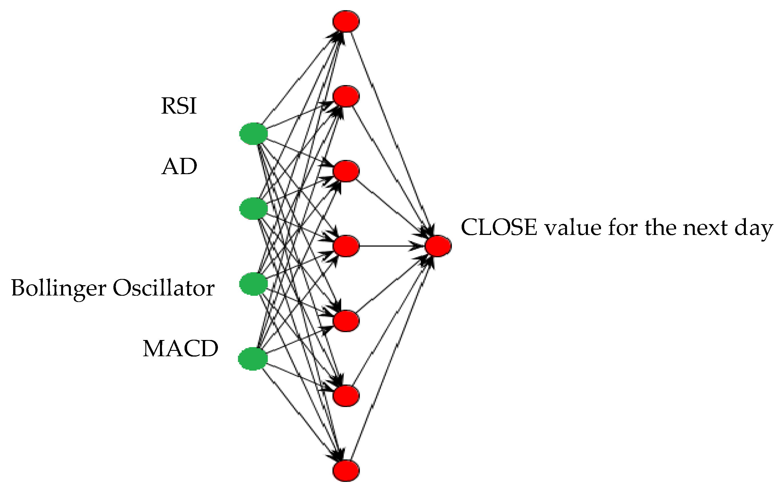
  • The relative strength index (RSI) is used to identify whether the market is overbought or oversold. The values are always in the range from 0 to 100. If the RSI is smaller than 30, it is assumed that the market is sold out, while a value larger than 70 means that the market is bought out. However, in the case of strong trends, RSI < 20 signifies a sold-out market (during a bear market) and RSI > 80 indicates a buyout market (during a bull market). The RSI is a measure of the strength of growth movements in relation to downward movements.

    $$\mathrm{RSI}(k)=100-\left[\frac{100}{1+\frac{{\mathrm{EMA}}_{N,U}(k)}{{\mathrm{EMA}}_{N,D}(k)}}\right],$$

    (4)

    where:
    U(k)—average increase on the k-th day, and for C(k) > C(k − 1), U(k) = C(k) − C(k − 1),
    D(k)—average decrease on the k-th day, and for C(k) < C(k − 1), D(k) = |C(k) − C(k − 1),
    EMA_N,U, EMA_N,D—exponential moving averages for N days and for U(k) or D(k), respectively.
  • The stochastic oscillator (K%D) determines the relative value of the last closing price in relation to the considered range of price changes in a given period. Oscillator values cover a range from 0 to 100. If K%D is over 70, that the closing price is considered to be near the top end of the range of its fluctuations. A K%D below 30 indicates that it is close to the lower end of that range.

    $$K\%D(k)=100\left[\frac{C(k)-L(14)}{H(14)-L(14)}\right],$$

    (5)

    where L(14) and H(14) are the lowest and highest prices, respectively, over the last 14 days.
  • The moving average convergence/divergence (MACD) is defined as the difference between the long-term and short-term values of exponential moving averages. This oscillator is used to study buy and sell signals. It is usually compared with its 9-day exponential moving average, which is called the signal line (SL). The intersection of these two signals indicates a buying signal if the MACD line comes from the bottom, and a selling signal if this line is from the top.

    MACD(k) = EMA_{12, C} (k) − EMA_26,C(k)

    (6)

    SL(k) = EMA₉(MACD(k))

    (7)
  • Accumulation/distribution (AD) relates to the price and volume and indicates whether the price changes in the stock market appear together with increased accumulation and distribution movements.

    $$AD(k)=V\left(k\right)\frac{C\left(k\right)-L\left(k\right)-\left[H\left(k\right)-C\left(k\right)\right]}{H\left(k\right)-L\left(k\right)}$$

    (8)

    where V(k) is a volume, e.g., the total number of shares traded on k-th day, and L(k) and H(k) are the lowest and the highest prices on k-th day.
  • The Bollinger oscillator (BOS) informs whether the market is overbought or oversold. It is derived from the Bollinger bands.

    $${\mathrm{BOS}}_C(k)=\frac{\mathrm{C}(k+N-1)-{\mathrm{SMA}}_{N,C}(k))}{\mathrm{SD}e{v}_C(k)},$$

    (9)

    where $\mathrm{SD}e{v}_C(k)$ denotes the standard deviation of C(k).

3. Fractal Analysis

Fractal-based approaches have been gaining popularity in market analyses. This is due to the fact that fractal analysis (FA) allows for more precise modeling of stock market trends than technical analysis. The implementation of fractal analysis requires recognition of the fractal dimension. For this purpose, we used the so-called box-counting procedure [38]. The analyzed data chart was covered by N small elements (boxes) of size S. If we change the scale and the size of elements from S₁ to S₂, the relationship between the number of elements N₁ and N₂ needed to cover the graph with objects of S₁ and S₂ size, respectively, is given as [42]:

$$\frac{N_2}{N_1}={\left(\frac{S_1}{S_2}\right)}^D,$$

(10)

$$D=\frac{\log \left(\frac{N_1}{N_2}\right)}{\log \left(\frac{S_1}{S_2}\right)}$$

(11)

where D denotes the fractal dimension.

When measuring the fractal dimension of the share prices chart, the considered period of time 2T should be divided into two equal intervals. For each time period, the chart of share prices is covered by N elements. The number N_1T of elements in the first time period T is equal to:

$$N_{1T}(k)=\frac{H_T(k)-L_T(k)}{T},$$

(12)

where H_T(k) and L_T(k) are the highest and lowest share prices in the first time period T.

The number N_2T of elements in the second time period T is equal to:

$$N_{2T}(k)=\frac{H_{2T}(k)-L_{2T}(k)}{T},$$

(13)

where H_2T(k) and L_2T(k) are the highest and the lowest share prices in the second time period from T to 2T.

The number N_0–2T of elements in the whole considered time period 2T is equal to:

$$N_{0-2T}(k)=\frac{H_{0-2T}(k)-L_{0-2T}(k)}{2T},$$

(14)

where H_0–2T(k) and L_0–2T(k) are the highest and the lowest share prices over the whole time period 2T.

The fractal dimension of the share price chart is given by the relationship [42]:

$$D=\frac{\log \left(\frac{N_{1T}+N_{2T}}{N_{(0-2)T}}\right)}{\log \left(\frac{2T}{T}\right)}=\frac{\log (N_{1T}+N_{2T})-\log (N_{(0-2)T})}{\log (2)}.$$

(15)

The fractal dimension is used to define the fractal moving average (FRAMA). This moving average is derived from the exponential moving average (Equation (2)) with (1 − a) coefficient, where a is given by [42]:

$$a=\exp (-4.6(D-1)).$$

(16)

In this paper, we extend the idea of using a fractal approach to predict share prices and propose new technical analysis indicators with FRAMA:

• The relative strength index with FRAMA (RSI_FRAMA)—this FA indicator is derived from the TA indicator RSI (Equation (4)) by replacing EMA with FRAMA.

  $${\mathrm{RSI}\_\mathrm{FRAMA}}_C(k)=100-\left[\frac{100}{1+\frac{{\mathrm{FRAMA}}_{N,U}(k)}{{\mathrm{FRAMA}}_{N,D}(k)}}\right],$$

  (17)

  where U(k) and D(k) are, respectively, the average increase and the average decrease on the k-th day.
• The moving average convergence/divergence with FRAMA (MACD_FRAMA)—this FA oscillator is based on MACD (Equation (6)) and SL (Equation (7)), as described in Section 3.

  MACD_FRAMA_C(k) = FRAMA_12,C(k) − FRAMA_26,C(k),

  (18)

  SL_F(k) = FRAMA_{9,MACD_FRAMA}(k),

  (19)

  where SL_F is the signal line with FRAMA.
• The Bollinger oscillator with FRAMA (BOS_FRAMA) is based on Bollinger bands. It is derived from the BOS given in Equation (9) by replacing SMA by FRAMA. This oscillator indicates when the market is overbought or oversold.

  $${\mathrm{BOS}\_\mathrm{FRAMA}}_C(k)=\frac{C(k+N-1)-{\mathrm{FRAMA}}_{N,C}(k)}{\mathrm{SD}e{v}_C(k)},$$

  (20)

  where $\mathrm{SD}e{v}_C(k)$ denotes the standard deviation.

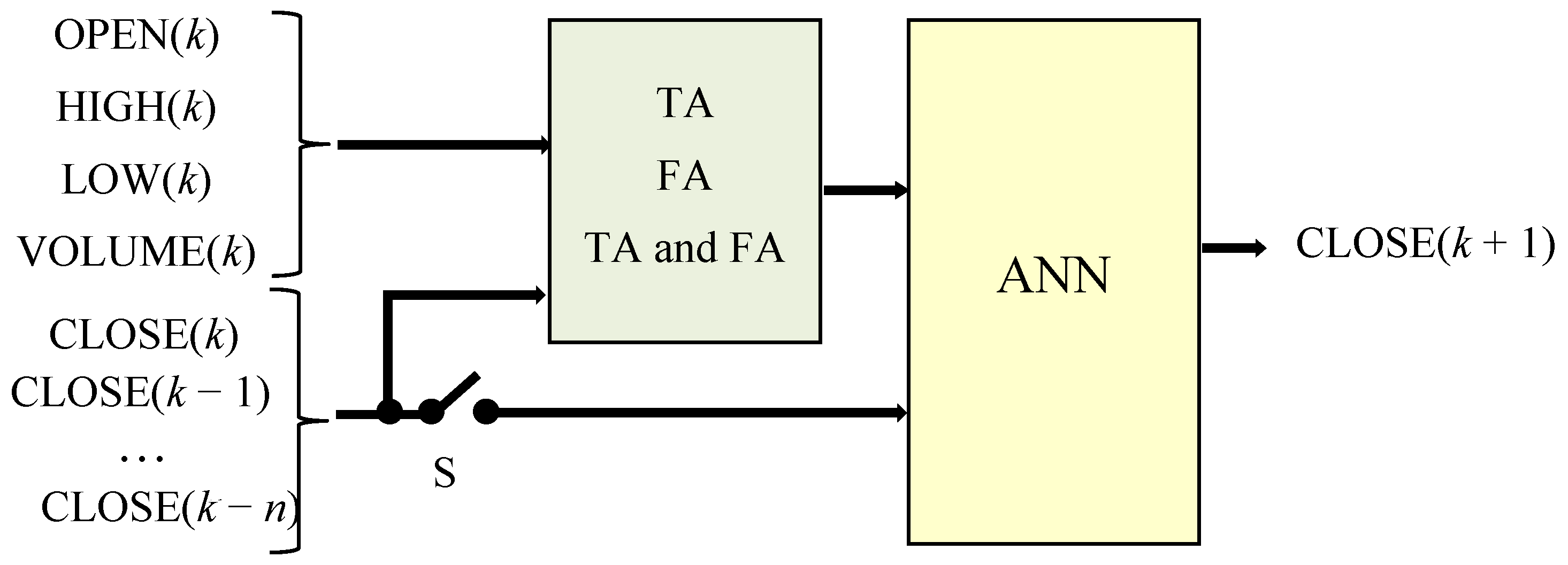
4. Application of Hybrid Analytical—Neural Models for Share Price Forecasting

Information regarding likely upcoming share price changes is of the utmost importance for investors. In this work, new hybrid analytical–neural models are proposed for predicting the closing price of an asset for the next day. In these models, technical or fractal analyses were combined with ANN. The general structure of these hybrid models is shown in Figure 1. In the first module, TA or FA indicators were calculated. These were then used as inputs for the ANN, and the share closing price for the next day was obtained as the ANN output. Three kinds of hybrid model are discussed:

• Hybrid models combining technical analysis and ANN (TA–ANN)
• Hybrid models combining fractal analysis and ANN (FA–ANN)
• Hybrid models combining technical and fractal analyses and ANN (TA–FA–ANN)

The different hybrid model structures were compared to find the best solution. The influence of fractal analysis on the final results was also examined.

In our earlier research, several TA–ANN models [22] and FA–ANN models [30] were tested, in which previously calculated market indicators were used as ANN inputs. This corresponds to the opened switch S, in Figure 1. In the present work, TA–FA–ANN models are introduced. A moving time window method was also applied in all three kinds of hybrid model, where, in addition to market indicators, the current and several past samples of the CLOSE signal were entered as ANN inputs. This variant corresponds to the closed switch S, in Figure 1.

Feed-forward ANNs of the MLP type were applied for close price forecasting. An example of one of the applied two-layer MLP structures is shown in Figure 2.

Figure 2 shows an exemplary architecture (4–7–1) of the studied networks. It is composed of 4 input nodes, 7 neurons with a sigmoidal transfer function in a hidden layer, and 1 neuron in an output layer. In this study, different two-layer MLP structures were tested with different numbers of inputs and neurons in the hidden layer. It was confirmed that such two-layer ANNs are universal approximators [13], i.e., they are capable of mapping any smooth input–output functions with appropriate accuracy [43]. In the presented example, four market indicators were entered into the ANN input and the CLOSE value was obtained on the ANN output. Generally, for all the tested ANNs, the number of inputs is determined by the number of implemented TA and FA indices and also by the number of CLOSE signal past samples. The number of neurons in the hidden layer should be chosen in such a way as to achieve a compromise between ANN accuracy and generalization capability [44]. An insufficient number of neurons would result in poor ANN accuracy. Too many neurons would increase the network training time and could cause losses in ANN generalization capability [44]. Therefore, different types of MLP were tested. The ANNs were trained with a resilient propagation algorithm [45]. Input variables were selected on the basis of expert knowledge gathered in a literature review [14,16,41,46,47] and then tested experimentally according to the rules described in Section 5. The main criterion for selecting the ANN structures was the minimum of the mean square error (MSE) for the testing data.

The reference method for hybrid modeling was a purely ANN-based approach, in which the moving time window method [48] was applied and the share close price was predicted by MLP.

5. Experimental Part

5.1. Methodology

Different hybrid models using TA, FA, and ANN were compared with a purely ANN-based approach, as well as to find the best solution for short-term CLOSE value prediction. For this purpose, specialized software was designed using Java and an Encog library, which allows both for stock data collection and pre-processing and also for training and testing automatically a large number of different hybrid model structures. In our previous study [22], the choice of ANN input variables was made on the basis of expert knowledge. A small number of input variables were selected in order to design sufficiently accurate yet compact models. In the present work, new algorithms were implemented to create different hybrid models with ANNs of two-layer MLP type (see Figure 2). A large number of market indicators in different configurations were considered. The ANN input variables were selected randomly and the most accurate model structures were identified in an experimental way, based on the results of machine learning. The main machine learning algorithm is based on the following rules:

• A set of ANN input data vectors (i.e., not repeated combinations of market indicators with or without CLOSE past samples for a selected company) is generated randomly.
• For each combination of input data, a set of MLP structures is generated and for n inputs, the number of neurons in the hidden layer is changed as follows: n + 1, 1.5n, 2n − 1, 2n + 1, 3n, where n = 4, 5, 6, 7, 8, 9, ...
• For each input vector and each MLP structure:
  • All input data are normalized to <0.1; 0.9> range using the following formula:

    Normalized_Value = 0.8 (Value/Value_max) + 0.1;

    (21)
  • The training data for each company are divided into a learning data set and a testing data set, where the testing set is about 30%;
  • The ANNs are trained using the resilient propagation algorithm with a momentum factor;
  • Eight different ANNs are trained and the ANN with the smallest MSE for the testing data is chosen as the best.
• From the whole set of trained ANNs, a small subset of the best ANNs is identified, for which the MSE for the testing data is smaller than the defined error limit.

The proposed stock exchange data forecasting methodology was tested on historical stock data for five chosen companies (ŻYWIEC SA, ASSECO POLAND SA, BANK BPH SA, BUDIMEX SA, and VISTULA SA). The tested companies represent different market sectors, so the results can be generalized. They have been listed on the Warsaw Stock Exchange (WSE) since at least 1999. The WSE has been running since 12 April 1991. All the ANNs were trained on data covering the period from the start of the company’s listing on the WSE to the end of 2008, and then tested on data from 1 January 2009 to 1 January 2015 (6 years).

The best hybrid model structures were selected in an experimental way according to the following scheme:

• First, 12,628 various input data vectors were generated randomly for one company. Then, 208,518 different MLPs were trained. Each network was trained according to the rules defined above.
• In the second step, 29,149 MLPs with the smallest MSE were selected and their structures used to train ANNs for three randomly chosen companies.
• Next, 5545 ANN structures with an MSE smaller than the defined error limit were used to train ANNs for all five companies.
• Finally, 300 ANNs with the lowest MSE for the testing data for all five companies were selected and used to predict close values for the next day.

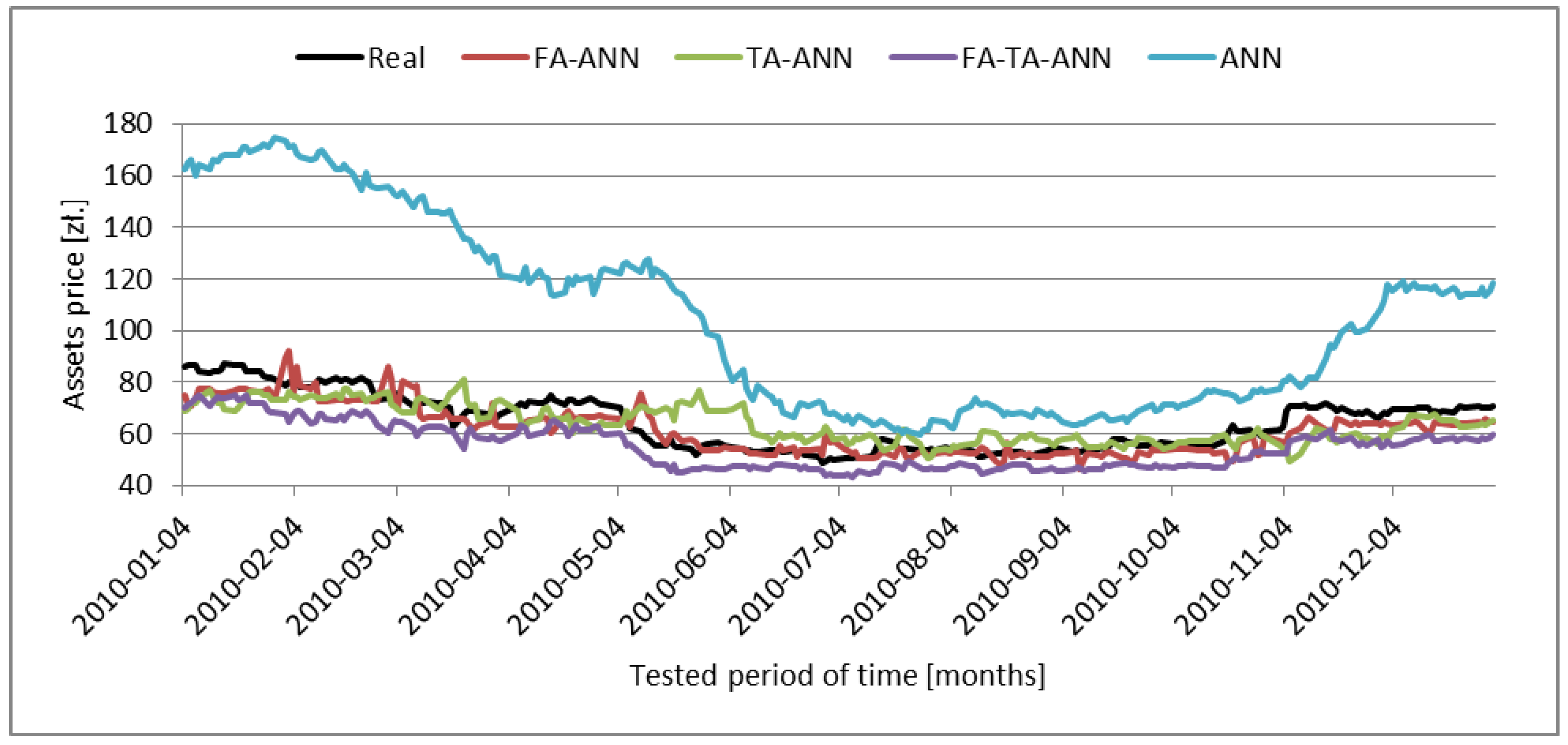
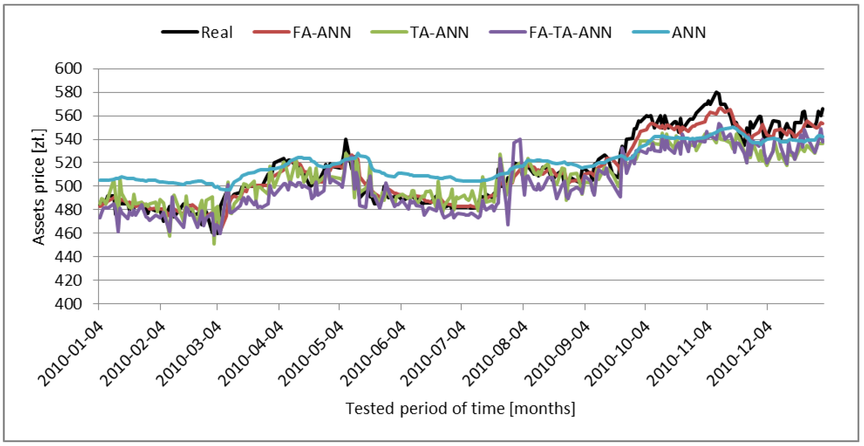
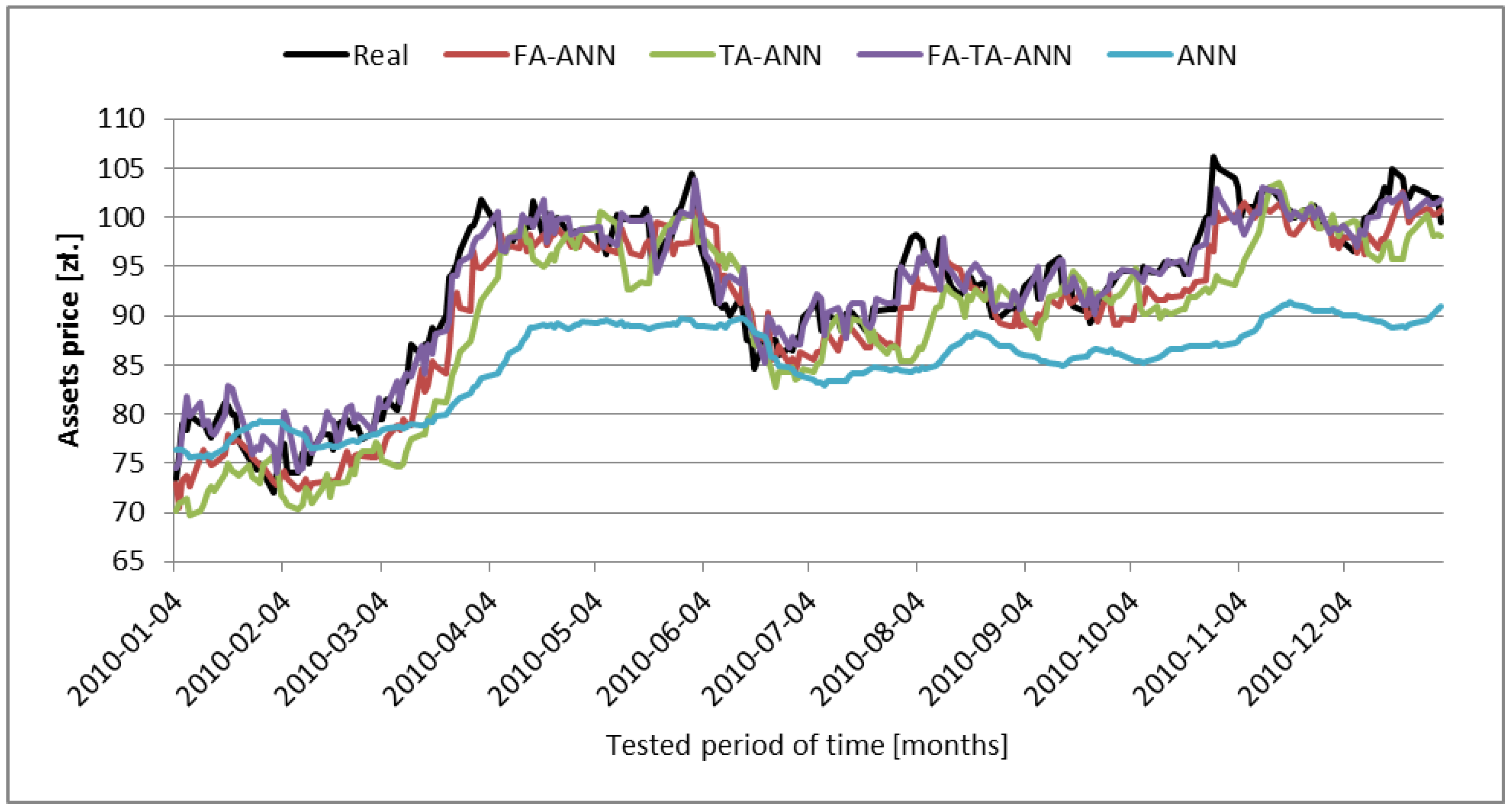
5.2. Results

The best networks for all types of the tested ANN-based hybrid models for the five chosen companies are listed in

Table 1. Selected ANN-based models: best prediction results for testing data.

Company	Model Structure	Type of ANN-Based Model
		FA–ANN	TA–ANN	FA–TA–ANN	ANN
ŻYWIEC	ANN structure	MLP(6–12–1)	MLP(22–33–1)	MLP(8–12–1)	MLP(8–17–1)
	Transfer function	sigmoidal	sigmoidal	Sigmoidal	Sigmoidal
	MSE	0.00013	0.00077	0.00041	0.00206
	ANN inputs	FRAMA10,C(k) FRAMA16,C(k) C(k − 1) … C(k − 4)	MACD(k) SMA5,C(k) LWMA5,C(k) LWMA10,C(k) LWMA20,C(k) TMA10,C(k) HULL20,C(k) HULL25,C(k) HULL30,C(k) RSI9,C(k) Williams_Indicator(k) CCI(k) Momentum20,C(k) ROC(k) EMA20,ROC(k) C(k − 1) … C(k − 7)	FRAMA10,C(k) FRAMA16,C(k) Volume Oscillator(k) SL9,MACD(k) FRAMA9,HL(k) LWMA10,C(k) LWMA20,C(k) ChaikinOscillator_FRAMA(k)	C(k − 1) … C(k − 8)
ASSECO POLAND	ANN structure	MLP(7–13–1)	MLP(13–27–1)	MLP(6–7–1)	MLP(9–13–1)
	Transfer function	sigmoidal	sigmoidal	Sigmoidal	Sigmoidal
	MSE	0.00003	0.0001	0.00003	0.00089
	ANN inputs	FRAMA10,C(k) FRAMA16,C(k) C(k − 1) … C(k − 5)	EMA5,C(k) EMA30,C(k) Ultimate_Oscillator CHL3 RSI9,C(k) HULL_RSI14,C(k) C(k − 1) … C(k − 7)	qStick_FRAMA SMA20,C(k) LWMA20,C(k) TMA5,C(k) TMA10,C(k) ROC(k)	C(k − 1) … C(k − 9)
BANK BPH	ANN structure	MLP(8–12–1)	MLP(13–27–1)	MLP(6–7–1)	MLP(25–51–1)
	Transfer function	sigmoidal	Hyperbolic tangent	Sigmoidal	Hyperbolic tangent
	MSE	0.00001	0.00007	0.00002	0.00045
	ANN inputs	FRAMA20,C(k) MACD_FRAMA(k) FRAMA9,HL(k) CCI_FRAMA(k) C(k − 1) … C(k − 4)	SMA10,C(k) LWMA20,C(k) Momentum20,C(k) Std_Dev_HuLL10,C(k) C(k − 1) … C(k − 9)	FRAMA10,C(k) FRAMA16,C(k) Detrend Price Oscillator5,C(k) Detrend Price Oscillator10,C(k) Detrend Price Oscillator20,C(k) Mass_Index25,C(k)	C(k − 1) … C(k − 25)
BUDIMEX	ANN structure	MLP(13–25–1)	MLP(15–22–1)	MLP(13–25–1)	MLP(14–15–1)
	Transfer function	sigmoidal	sigmoidal	Sigmoidal	Sigmoidal
	MSE	0.00175	0.00288	0.00165	0.00986
	ANN inputs	FRAMA10,C(k) FRAMA16,C(k) BOS_FRAMA20,C(k) Chaikin Volatility_FRAMA(k) C(k − 1) … C(k − 9)	EMA5,C(k) EMA10,C(k) HULL_RSI9,C(k) Detrend Price Oscillator5,C(k) Mass_Index25,C(k) Profitability Index Rule14,C(k) C(k − 1) … C(k − 9)	FRAMA16,C(k) EMA5,C(k) EMA10,C(k) EMA30,C(k) FRAMA20,C(k) SL9,MACD(k) MACD_FRAMA(k) Fractal Dimension5,C(k) Fractal Dimension16,C(k) SMA20,C(k) HULL25,C(k) FRAMA5,C(k) CCI_FRAMA(k)	C(k − 1) … C(k − 14)
VISTULA	ANN structure	MLP(10–15–1)	MLP(13–27–1)	MLP(13–14–1)	MLP(15–22–1)
	Transfer function	sigmoidal	sigmoidal	Sigmoidal	Sigmoidal
	MSE	0.00003	0.00013	0.00004	0.00056
	ANN inputs	FRAMA10,C(k) FRAMA16,C(k) AverageTrueRange_FRAMA(k) Chaikin Volatility_FRAMA(k) C(k − 1) … C(k − 6)	EMA25,C(k) SL9,MACD(k) LWMA10,C(k) HULL30,C(k) CCI(k) ROC(k) Volume_ROC(k) Freedom of Movement Indicator(k) EMA20,ROC(k) C(k − 1) … C(k − 4)	FRAMA16,C(k) EMA10,C(k) EMA30,C(k) CHL(k), MACD_FRAMA(k) LWMA5,C(k) EMA9,HL(k) TMA5,C(k) HULL30,C(k) Stochastic Oscillator_W3,C(k) ROC(k) Volume_ROC(k) Chaikin Oscillator_FRAMA(k)	C(k − 1) … C(k − 15)

. The best ANN-based hybrid models in each of the considered classes of models are shown. It can be noted that for the FA–ANN and TA–ANN models, the structures with inputs extended by current and past samples of the CLOSE signal (closed switch S, in Figure 1) produced the best results (i.e., the smallest MSE for the testing data covering a period of 6 years).

Comparison of the MSE obtained for the testing data implies that hybrid models ensure better accuracy than a purely ANN-based approach. The hybrid model with fractal analysis outperforms the hybrid model with only TA and its results are similar to those of models with technical and fractal analysis indicators as input for the ANNs.

The MSE is a commonly used criterion for evaluating the accuracy of models, yet it averages the results. Therefore, the time series of the close prices of the considered companies was analyzed in detail. The results indicate that information from a single ANN is an insufficient basis for investment decisions. Therefore, in order to find the best hybrid ANN-based model, four kinds of model with the smallest MSE listed in Table 1 were tested for all five considered companies. Because the testing time period of 6 years is too long to observe the complete time series charts, it was shortened to one year only—2010. One year is long enough for the results to be representative for the whole set of the tested companies over a long period of time. Exemplary results of CLOSE price predictions obtained for three selected companies are presented in Figure 3, Figure 4 and Figure 5.

A comparison of the results shows that CLOSE value predictions using the hybrid ANN-based approach with technical and fractal analyses are more stable over a long period of time than those using the ANN model. The best prediction accuracy was obtained for the FA–ANN and FA–TA–ANN models.

The most important prediction parameter for investors is the highest absolute error. For the purposes of comparison, the following error measures were used:

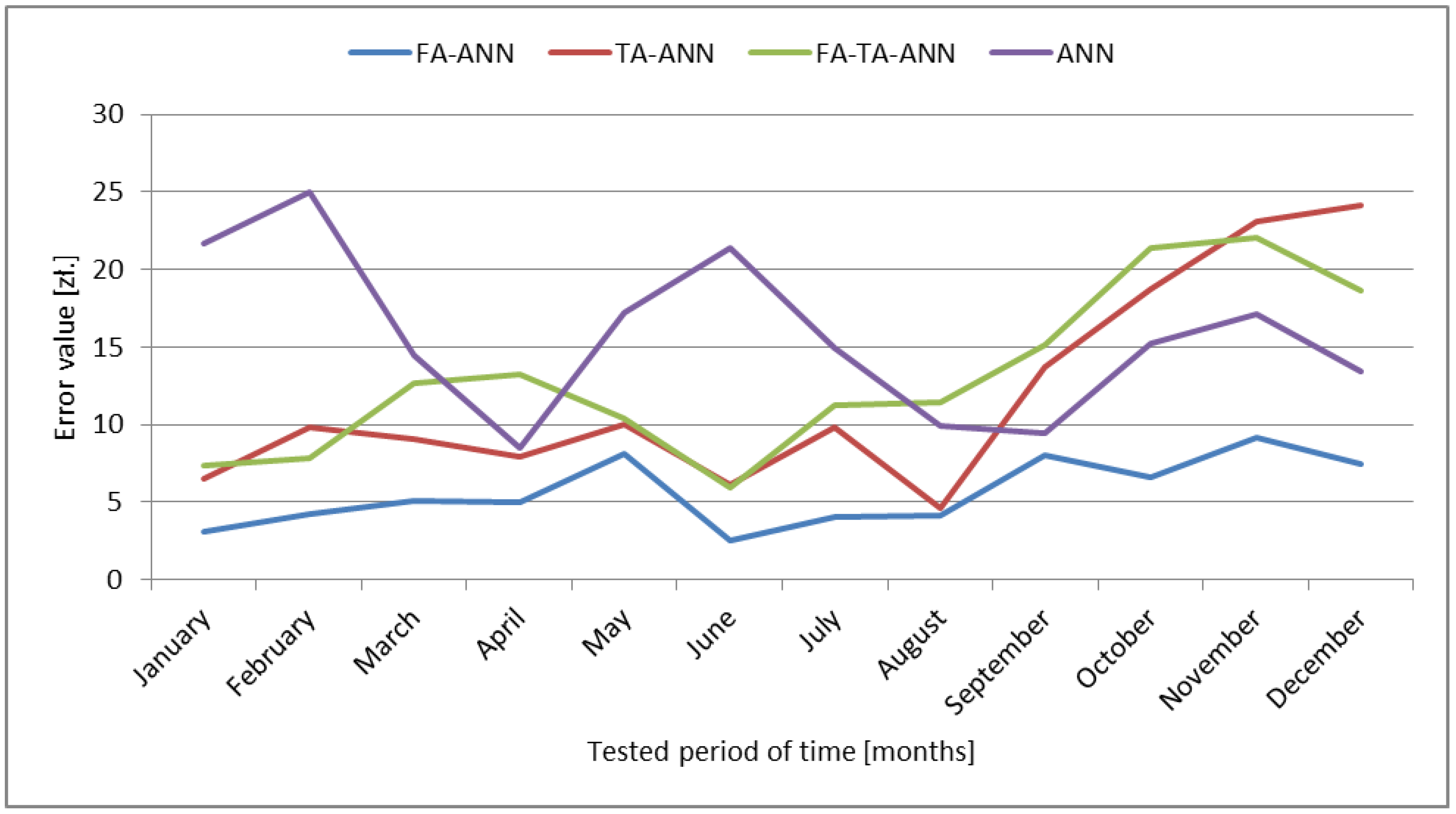
• The highest prediction error per month E_max—i.e., the highest difference between the real CLOSE value and the value predicted by the ANN per month:

  $$E_{\mathit{max}}=\mathit{max}\left|C(k)-\widehat{C}(k)\right|,\mathrm{for}k=1,2,\dots ,N.$$

  (22)
• Arithmetical mean of the month E_max values per tested period of time (one year):

  $$\overline{E_{\mathit{max}}}=\frac{1}{N}{\displaystyle {\sum }_{i=1}^N{E}_{{\mathit{max}}_i}}.$$

  (23)

These error measures were used in the assessment and validation of the tested models.

In order to assess the precision and stability of the models, the maximum absolute errors E_max of one day-ahead predictions were calculated from Equation (22) for each month in the test period. The results obtained for ŻYWIEC SA in the period of one year for the ANN-based model and three hybrid models are given in Figure 6. Analogical results obtained for BPH Bank SA are shown in Figure 7 and for BUDIMEX SA in Figure 8.

The results shown in Figure 6, Figure 7 and Figure 8 imply that the hybrid approach using technical analysis with fractal indicators combined with the ANN (FA–ANN) ensured the best accuracy in terms for short-term predictions of CLOSE values. The worst results were obtained with the purely ANN-based approach. Similar results were obtained for other tested companies.

A comparison of the arithmetical means $\overline{E_{\mathit{max}}}$ of monthly E_max errors (absolute and relative) in the tested period of one year (2010) for the five selected companies and for four kinds of ANN-based models is presented in

Table 2. Arithmetical means of monthly E_max values (absolute and relative) for one year (2010).

Company	FA–ANN		TA–ANN		TA–FA–ANN		ANN
	$\overline{{\mathit{E}}_{\mathit{max}}}$ (PLN)	$\mathsf{\delta }\overline{{\mathit{E}}_{\mathit{max}}}$ (%)	$\overline{{\mathit{E}}_{\mathit{max}}}$ (PLN)	$\mathsf{\delta }\overline{{\mathit{E}}_{\mathit{max}}}$ (%)	$\overline{{\mathit{E}}_{\mathit{max}}}$ (PLN)	$\mathsf{\delta }\overline{{\mathit{E}}_{\mathit{max}}}$ (%)	$\overline{{\mathit{E}}_{\mathit{max}}}$ (PLN)	$\mathsf{\delta }\overline{{\mathit{E}}_{\mathit{max}}}$ (%)
BPH BANK	4.73	7.35	6.63	10.8	9.47	14.85	40.92	74.37
ŻYWIEC	5.61	1.09	11.95	2.34	13.11	2.58	15.68	3.13
VISTULA	0.10	3.88	0.13	5.35	0.12	4.85	0.61	24.56
BUDIMEX	2.65	2.89	3.93	4.39	1.4	1.58	7.57	8.24
ASSECOPOL	0.81	1.46	1.87	3.33	0.98	1.73	5.16	9.32

. These results confirm that the best accuracy was achieved by the hybrid model combining TA, FA, and ANN and the worst using the purely ANN-based approach.

6. Discussion and Conclusions

In this paper, new structures of hybrid ANN-based models combined with fractal analysis have been proposed for predicting stock exchange share values for the next day. Three kinds of hybrid models were compared. The first combines technical analysis and an ANN. The second combines technical and fractal analyses with an ANN. The third combines fractal analysis with an ANN. The aim was to identify the best model structure. Hybrid ANN-based models combining technical analysis and fractal analysis gave more precise short-term forecasts than the purely ANN-based approach. As can be seen from the results displayed in Table 1 and Table 2, the highest precision was achieved by the FA–ANN and TA–FA–ANN models. Marginally worse results were obtained with the TA–ANN model. The worst results were obtained using the purely ANN-based approach. Comparison of the E_max values for the audited period from January to December 2010 given in Figure 6, Figure 7 and Figure 8 reveals that the proposed hybrid ANN-based prediction models were more accurate over time than the ANN approach. Because technical and fractal analysis are incorporated into the proposed hybrid modeling schemes, the hybrid models were less vulnerable to false signals from the market. The hybrid ANN-based models with fractal analysis produced the best accuracy, and may offer a very useful tool for supporting stock brokers and investors in their decisions.

References

1. Malkiel, B.G. A Random Walk Down Wall Street, 6th ed.; W.W. Norton & Company, Inc.: New York, NY, USA, 1973. [Google Scholar]
2. Fama, E. Efficient Capital Markets: A Review of Theory and Empirical Work. J. Financ. 1970, 25, 383–417. [Google Scholar] [CrossRef]
3. Jegadeesh, N.; Titman, S. Profitability of Momentum Strategies: An evaluation of alternative explanations. J. Financ. 2001, 56, 699–720. [Google Scholar] [CrossRef]
4. Lo, A.W.; Mackinlay, A.C. A Non-Random Walk Down Wall Street, 5th ed.; Princeton University Press: Princeton, NJ, USA, 2002; pp. 4–47. [Google Scholar]
5. Granger, C.W.J.; Morgenstern, O. Spectral Analysis of New York Stock Market Prices. Kyklos 2007, 16, 1–27. [Google Scholar] [CrossRef]
6. Guido, R.C.; Barbon, S., Jr.; Vieira, L.S.; Sanchez, F.L.; Maciel, C.D.; Pereira, J.C.; Scalassara, P.R.; Fonseca, E.S. Introduction to the discrete shapelet transform and a new paradigm: Joint time-frequency-shape analysis. In Proceedings of the IEEE International Symposium on Circuits and Systems (IEEE ISCAS 2008), Seattle, WA, USA, 18–21 May 2008; Volume 1, pp. 2893–2896. [Google Scholar]
7. Witkowska, D. Artificial Neural Networks and Statistical Methods. Selected Financial Issues; C. H. Beck: Warsaw, Poland, 2002. [Google Scholar]
8. Box, G.E.P.; Jenkins, G.M. Time Series Analysis. Forecasting and Control; Holden-Day Inc.: San Francisco, CA, USA, 1976. [Google Scholar]
9. Dębski, W. Financial Market and It Mechanisms; PWN: Warsaw, Poland, 2010. (In Polish) [Google Scholar]
10. Sutheebanjard, P.; Premchaiswadi, W. Stock Exchange of Thailand Index Prediction Using Back Propagation Neural Networks. In Proceedings of the Second International Conference on Computer and Network Technology (ICCNT), Bangkok, Thailand, 23–25 April 2010; pp. 377–380. [Google Scholar] [CrossRef]
11. Tilakaratne, C.D.; Morris, S.A.; Mammadov, M.A.; Hurst, C.P. Predicting Stock Market Index Trading Signals Using Neural Networks. In Proceedings of the 14th Annual Global Finance Conference (GFC 2007), Melbourne, Australia, September 2007; pp. 171–179. [Google Scholar]
12. Zhou, X.S.; Dong, M. Can fuzzy logic make technical analysis 20/20? Financ. Anal. J. 2004, 60, 54–75. [Google Scholar] [CrossRef]
13. Hornik, K.; Stinchcombe, M.; White, H. Multilayer Feedforward Networks are Universal Approximators. Neural Netw. 1990, 3, 551–560. [Google Scholar] [CrossRef]
14. Gately, E. Neural Networks for Financial Forecasting; Wiley: New York, NY, USA, 1995. [Google Scholar]
15. Hamzacebi, C.; Akay, D.; Kutay, F. Comparison of direct and iterative artificial neural network forecast approaches in multi-periodic time series forecasting. Expert Syst. Appl. 2009, 36, 3839–3844. [Google Scholar] [CrossRef]
16. Zieliński, J. Intelligent Management Systems—Theory and Practice; PWN: Warsaw, Poland, 2000. (In Polish) [Google Scholar]
17. Ghiassi, M.; Saidane, H.; Zimbra, D.K. Dynamic artificial neural network model for forecasting time series events. Int. J. Forecast. 2005, 21, 341–362. [Google Scholar] [CrossRef]
18. Majhi, R.; Panda, G.; Sahoo, G. Efficient prediction of exchange rates with low complexity artificial neural network models. Expert Syst. Appl. 2009, 36, 181–189. [Google Scholar] [CrossRef]
19. Brdyś, M.A.; Borowa, A.; Idźkowiak, P.; Brdyś, M.T. Adaptive Prediction of Stock Exchange Indices by State Space Wavelet Networks. Int. J. Appl. Math. Comput. Sci. 2009, 19, 337–348. [Google Scholar] [CrossRef] [Green Version]
20. Hajto, P. A Neural Economic Time Series Prediction with the Use of a Wavelet Analysis. Schedae Inform. 2002, 11, 115–132. [Google Scholar]
21. Tadeusiewicz, R. Discovering Neural Networks Using Programs in C# Programming Language; Polska Akademia Umiejętności: Cracow, Poland, 2007. (In Polish) [Google Scholar]
22. Paluch, M.; Jackowska-Strumiłło, L. Prediction of closing prices on the Stock Exchange with the use of artificial neural networks. Image Process. Commun. 2012, 17, 275–282. [Google Scholar] [CrossRef]
23. Zhang, G.P. Time series forecasting using a hybrid ARIMA and neural network model. Neurocomputing 2003, 50, 159–175. [Google Scholar] [CrossRef]
24. Khashei, M.; Bijari, M. An artificial neural network (p, d, q) model for time series forecasting. Expert Syst. Appl. 2010, 37, 479–489. [Google Scholar] [CrossRef]
25. Güresen, E.; Kayakutlu, G. Forecasting Stock Exchange Movements Using Artificial Neural Network Models and Hybrid Models. In Intelligent Information Processing IV, Proceedings of the IFIP International Federation for Information Processing, Beijing, China, 19–22 October 2008; Shi, Z., Mercier-Laurent, E., Leake, D., Eds.; Springer: Boston, MA, USA, 2008; Volume 288, pp. 129–137. [Google Scholar]
26. Güresen, E.; Kayakutlu, G.; Daim, T.U. Using artificial neural network models in stock market index prediction. Expert Syst. Appl. 2011, 38, 10389–10397. [Google Scholar] [CrossRef]
27. Witkowska, D.; Marcinkiewicz, E. Construction and Evaluation of Trading Systems: Warsaw Index Futures. Int. Adv. Econ. Res. 2005, 11, 83–92. [Google Scholar] [CrossRef]
28. Faustryjak, D.; Majchrowicz, M.; Jackowska-Strumiłło, L. Web System Supporting Stock Prices Analysis. In Proceedings of the International Interdisciplinary PhD Workshop 2017 (IIPhDW 2017), Lodz, Poland, 9–11 September 2017; pp. 157–163, ISBN 978-83-7283-858-2. [Google Scholar]
29. Faustryjak, D.; Jackowska-Strumiłło, L.; Majchrowicz, M. Forward Forecast of Stock Prices Using LSTM Neural Networks with Statistical Analysis of Published Messages. In Proceedings of the International Interdisciplinary PhD Workshop 2018 (IIPhDW 2018), Świnoujście, Poland, 9–12 May 2018; pp. 288–292. [Google Scholar] [CrossRef]
30. Paluch, M.; Jackowska-Strumiłło, L. The influence of using fractal analysis in hybrid MLP model for short-term forecast of close prices on Warsaw Stock Exchange. In Proceedings of the Federated Conference on Computer Science and Information Systems 2014, FedCSIS 2014, Warsaw, Poland, 7–10 September 2014; pp. 111–118. [Google Scholar] [CrossRef]
31. Jackowska-Strumiłło, L. Hybrid Analytical and ANN-based Modelling of Temperature Sensors Nonlinear Dynamic Properties. In Lecture Notes in Artificial Intelligence, Proceedings of the 6th International Conference on Hybrid Artificial Intelligence Systems, HAIS 2011, Wroclaw, Poland, 23–25 May 2011; LNAI 6678; Springer: Berlin, Germany, 2011; Part I; pp. 356–363. [Google Scholar] [CrossRef]
32. Jackowska-Strumillo, L.; Cyniak, D.; Czekalski, J.; Jackowski, T. Neural model of the spinning process dedicated to predicting properties of cotton-polyester blended yarns on the basis of the characteristics of feeding streams. Fibres Text. East. Eur. 2008, 16, 28–36. [Google Scholar]
33. Paluch, M.; Jackowska-Strumiłło, L. Intelligent information system for stock exchange data processing and presentation. In Proceedings of the 8th International Conference on Human System Interaction (HSI 2015), Warszawa, Poland, 25–27 June 2015; pp. 238–243. [Google Scholar] [CrossRef]
34. Paluch, M.; Jackowska-Strumiłło, L. Decision system for stock data forecasting based on Hopfield artificial neural network. Inform. Control Measure. Econ. Environ. Protect. 2016, 6, 28–33. [Google Scholar] [CrossRef]
35. Paluch, M.; Jackowska-Strumiłło, L. Intelligent Decision System for Stock Exchange Data Processing and Presentation. In Human-Computer Systems Interaction. Backgrounds and Applications 4; Series: Advances in Intelligent Systems and Computing; Hippe, Z.S., Kulikowski, J.L., Mroczek, T., Eds.; Springer International Publishing AG: Cham, Switzerland, 2018; Volume 551, pp. 80–90. [Google Scholar] [CrossRef]
36. Drabik, E. Applications of Game Theory to Invest in Securities; Wydawnictwo Uniwersytetu w Białymstoku: Białystok, Poland, 2000. (In Polish) [Google Scholar]
37. Ehlers, J. Fractal Adaptive Moving Average; Technical Analysis of Stock & Commodities: Seattle, WA, USA, 2005. [Google Scholar]
38. Guariglia, E. Entropy and Fractal Antennas. Entropy 2016, 18, 84. [Google Scholar] [CrossRef]
39. Guariglia, E. Harmonic Sierpinski Gasket and Applications. Entropy 2018, 20, 714. [Google Scholar] [CrossRef]
40. Berry, M.V.; Lewis, Z.V. On the Weierstrass-Mandelbrot fractal function. Proc. R. Soc. Lond. Ser. A 1980, 370, 459–484. [Google Scholar] [CrossRef]
41. Murphy, J.J. Technical Analysis of Financial Markets; Wig-Press: Warsaw, Poland, 2008. (In Polish) [Google Scholar]
42. Ehlers, J. Cybernetics Analysis for Stocks and Futures; John Wiley & Sons: New York, NY, USA, 2004. [Google Scholar]
43. Rutkowski, L. Methods and Techniques of Artificial Intelligence; PWN: Warsaw, Poland, 2009. (In Polish) [Google Scholar]
44. Tadeusiewicz, R. Artificial Neural Networks; Akademicka Oficyna Wydawnicza RM: Warsaw, Poland, 1993. (In Polish) [Google Scholar]
45. Garcia, M.A.; Trinh, T. Detecting Simulated Attacks in Computer Networks Using Resilient Propagation Artificial Neural Networks. Polibits 2015, 51, 5–10. [Google Scholar] [CrossRef] [Green Version]
46. Bensignor, R. New Concepts in Technical Analysis; Wig-Press: Warsaw, Poland, 2004. (In Polish) [Google Scholar]
47. Bulkowski, T.N. Formation Analysis on Stock Charts; Linia: Warsaw, Poland, 2011. (In Polish) [Google Scholar]
48. Narendra, K.S.; Parthasarathy, K. Identification and control of dynamics systems using neural networks. IEEE Trans. Neural Netw. 1990, 1, 4–27. [Google Scholar] [CrossRef] [PubMed]
Figure 1. Processing scheme for one-day ahead predicting of the CLOSE value using hybrid TA–FA–ANN-based approach. TA = Technical analysis, FA = Fractal analysis, ANN = Artificial neural network.
Applsci 08 02473 g001
Figure 2. Example of multilayer perceptron (MLP) network featuring 4 inputs, 7 neurons in the hidden layer and a single output. RSI = Relative strength index, AD = Accumulation/distribution, MACD = Moving average convergence/divergence.
Applsci 08 02473 g002
Figure 3. Short-term forecast of ANN-based models and the real CLOSE value for BPH Bank SA in 2010.
Applsci 08 02473 g003
Figure 4. Short-term forecast of ANN-based models and the real CLOSE value for ŻYWIEC SA in 2010.
Applsci 08 02473 g004
Figure 5. Short-term forecast of ANN-based models and the real CLOSE value for BUDIMEX SA in 2010.
Applsci 08 02473 g005
Figure 6. Comparison of Emax values per month between all ANN-based models in a period of one year (2010) for ŻYWIEC SA.
Applsci 08 02473 g006
Figure 7. Comparison of Emax values per month using ANN-based models over one year (2010) for BPH Bank SA.
Applsci 08 02473 g007
Figure 8. Comparison of Emax values per month using all ANN-based models over one year (2010) for BUDIMEX SA.
Applsci 08 02473 g008